4

Background: Mathematical Research Areas Important for the Grid

INTRODUCTION

Building on the electric grid basics presented in Chapters 1 and 2 and the existing analytic methods from Chapter 3, this chapter covers the key mathematical research areas associated with the electric grid. As was the case in the previous chapters, the scope of the electric power industry and its wide variety of challenges mean that only the key mathematical techniques can be touched on.

The mathematical sciences provide essential technology for the design and operation of the power grid. Viewed as an enormous electrical network, the grid’s purpose is to deliver electrical energy from producers to consumers. The physical laws of electricity yield systems of differential equations that describe the time-varying currents and voltages within the system. As described in Chapter 1, the North American grid is operated in regimes that maintain the system close to a balanced three-phase, 60-Hz ideal. Conservation of energy is a fundamental constraint: Loads and generation must always balance. This balance is maintained in today’s network primarily by adjusting generation. Generators are switched on and off while their output is regulated continuously to match power demand. Additional constraints come from the limited capacity of transmission lines to deliver power from one location to another.

The character, size, and scope of power flow equations are daunting, but (approximate) solutions must be found to maintain network reliability. From a mathematical perspective, the design and operation of the grid is a two-step process. The first step is to design the system so that it will operate reliably. Here, differential equations models are formulated, numerical methods are used for solving them, and geometric methods are used for interpreting the solutions. The next section, “Dynamical Systems,” briefly introduces dynamical systems theory, a branch of mathematics that guides this geometric analysis. Stability is essential, and much of the engineering of the system is directed at ensuring stability and reliability in the face of fluctuating loads, equipment failures, and changing weather conditions. For example, lightning strikes create large, unavoidable disturbances with the potential to abruptly move the system state outside its desired operating regime and to permanently damage parts of the system. Control theory, introduced in a later section, “Control,” is a field that develops devices and algorithms to ensure stability of a system using feedback. In that section the committee describes some of the basic types of control that are currently used on the grid.

More generation capacity is needed than is required to meet demand, for two reasons: (1) loads fluctuate and can be difficult to accurately predict and (2) the network should be robust in the face of failures of network components. The organizations and processes used to regulate which generation sources will be used at any given time

were covered in earlier chapters. Key to this operation and its associated design is extensive use of optimization algorithms. The next section, “Optimization,” describes some of the mathematics and computational methods for optimization that are key aspects of this process. Because these algorithms sit at the center of wholesale electricity markets, they influence financial transactions of hundreds of millions of dollars daily.

The electrical grid operates 24/7, but its physical equipment has a finite lifetime and occasionally fails. Although occasional outages in electric service are expected, an industry goal is to minimize these and limit their extent. Cascading failures that produce widespread blackouts are disruptive and costly. Systematic approaches to risk analysis, described in the section “Risk Analysis, Reliability, Machine Learning, and Statistics,” augment physical monitoring devices to anticipate where failures are likely and to estimate the value of preventive maintenance.

The American Recovery and Reinvestment Act of 2009 funded the construction and deployment of many of the phasor measurement units (PMUs) discussed in Chapter 1, so that by 2015 there are approximately 2,000 production-grade PMUs just in North America that are sampling the grid 30 to 60 times per second (NASPI, 2015). This is producing an unprecedented stream of data, reporting currents and voltages across the power system with far greater temporal resolution (once every 4 to 6 seconds) than was available previously from the existing Supervisory Control and Data Acquisition (SCADA) systems. The subsections in “Complexity and Model Reduction in the Time of Big Data” discuss evolving areas of mathematics that seem likely to contribute to effective utilization of these new data. The last subsection discusses data assimilation, which has become an important tool for weather forecasting and may have application to the grid. Data assimilation enables the ongoing aggregation of weather observations into large numerical models that simulate the global evolution of the atmosphere to produce weather forecasts. Initialized with typical observational data, these computer models have very fast transients that in the real atmosphere have already decayed. One of the primary goals of data assimilation is to avoid these transients while still using the observational data. Data assimilation has yet to be tried on simulations of the electric grid, but the prospect of doing so is attractive. Methods for determining the extent to which a system with a large number of degrees of freedom behaves like a system with many fewer degrees of freedom are also discussed in the section “Complexity and Model Reduction in the Time of Big Data.” The prospect of applying these methods to the data from the PMUs is also very attractive.

The final section, “Uncertainty Quantification,” introduces mathematical methods for quantifying uncertainty. This area of mathematics is largely new, and the committee thinks that it has much to contribute to electric grid operations and planning. There are several kinds of uncertainty that affect efforts to begin merging real-time simulations with real-time measurements. These include the effects of modeling errors and approximations as well as the intrinsic uncertainty inherent in the intermittency of wind and solar generation and unpredictable fluctuations of loads. Efforts to create smart grids in which loads are subject to grid control and to generation introduce additional uncertainty. Hopefully, further development of smart grids will be able to exploit mathematical methods that quantify this uncertainty.

Some of the uncertainty associated with the next-generation grid is quite deep, in the sense that there is fundamental disagreement over how to characterize or parameterize uncertainty. This can be the case in situations such as predictions associated with solar or wind power, or risk assessments for high-impact, low-frequency events; with economic models that can be used to evaluate electricity markets or set rational pricing schemes for grid-connected distributed resources; or methods of assimilating peta-scale (or larger) data sets from distribution grids to help inform utility or consumer decision making and manage stochastic resources. The committee hopes that research into uncertainty quantification will extend to the development of new mathematical models to evaluate decisions made in the face of deep uncertainties. Existing decision models for power system planning, and existing economic models of electricity markets, have a very difficult time incorporating relevant time dimensions of any order.

The material in this chapter is intended to present sufficient background about these mathematical areas to understand important issues raised in their application to the power grid, building on the power grid material presented in Chapters 1 to 3. Chapter 5, Preparing for the Future, discusses challenges that the next-generation grid will present requiring new mathematical analysis, and Chapter 6, Mathematical Research Priorities Arising from the Electric Grid, discusses the new mathematical capabilities required to meet these challenges. Chapter 7’s goal is to illustrate some current mathematical and computational techniques in greater detail than could be captured

in earlier chapters in the form of case studies of the main challenges for mathematical and computational sciences created by ongoing changes in the power industry. Readers may wish to go directly to these descriptions, referring back to this chapter and earlier chapters when additional background material is needed. Finally, the committee notes here that differences in terminology between mathematics and power systems engineering sometimes cause confusion when the same word is given different meanings or when the same concept is described using different terminology. A simple example is the imaginary unit, which is i in mathematics and j in power engineering. This report attempts to give appropriate translations between the two fields.

DYNAMICAL SYSTEMS

Dynamical systems model the changes in time of interacting quantities. For electrical circuits, these quantities are the voltages and currents associated with the components of the network. As discussed in Chapter 1, power systems have many different time scales that need to be modeled as dynamical systems. Differential equations derived from the physical laws of electricity describe the rates of change of the variables. Kirchhoff’s laws for currents and voltages in an electrical network, together with models for network devices like generators, transformers, and motors, are the core ingredients for models of the electric grid. System dynamics can be simulated by solving these equations with analytical or numerical methods to obtain the solution that begins with a specified initial condition. Usually, this process is repeated for many different initial conditions of the variables and values of the parameters that appear in the equations defining the system. The transient stability (TS) analysis for power systems, covered in Chapters 1 and 3, is one example that utilizes these types of simulations. Following a contingency, which might be a fault due to an equipment failure or a discrete control action that switches equipment off or on, the system has a transient response that (hopefully) leads to a new stable operating point. Another example is the faster electromagnetic transients analysis covered in Chapter 3. For both there are many levels of models that can be simulated, and an ever present question is whether the dynamical properties of coarser and finer models are consistent with one another.

Dynamical systems theory goes further and provides a language for interpreting and understanding simulation results. This theory emphasizes qualitative properties of solutions and long-time behavior. Guckenheimer and Holmes (1983) offer one among many introductions to this subject. They view a solution as a point moving in an abstract phase space of all possible values. The path traced along the solution is a trajectory. Where do trajectories ultimately go? Different patterns are possible. For example, the system may approach an equilibrium where the variables remain constant in time or a periodic orbit where they regularly return to values they have had previously. Both types of behavior are immediately relevant to power systems. More complicated quasiperiodic or chaotic asymptotic states are found in many systems, and the study of their statistical properties has been another focus of the theory. Stability is a central concern: If the asymptotic state is perturbed, does the system return to its previous behavior? One goal of the theory is to produce a phase portrait that depicts which trajectories have the same asymptotic states.

Structural stability is a further question of interest: If system parameters are varied, does the phase portrait have the same topology? For equilibrium points and periodic orbits of a structurally stable system, linearization produces eigenvalues that determine their stability. An equilibrium is linearly stable if all of its eigenvalues have negative real parts. In the power systems literature, this is referred to as dynamic stability. The basin of attraction of a stable equilibrium determines which perturbations of the state of the system produce trajectories that return to that equilibrium. The stable manifold theorem gives further information about equilibria and periodic orbits that are not attractors, which is useful in computing phase portraits and basin boundaries. Thus the basic question investigated by TS analysis is whether postfault states of a system lie in the basin of attraction of a desired attracting state. If not, control action that steers the system into this region is needed.

The ac design of the electrical grid presents a modeling challenge. The transmission grid has important time scales of minutes to hours that are much slower than the 60-Hz ac oscillations. Models that explicitly represent the ac oscillations have no equilibria; their simplest attractors are periodic orbits with a period of 1/60 sec. In averaged systems liked those used in power flow they become equilibria. This makes analysis significantly more difficult because finding equilibria requires the solution of only algebraic rather than differential equations. Simulation is

also more difficult because numerical methods must use small time steps that are able to track the rapid oscillations. Consequently, models that average these oscillations are commonly employed. The averaging process is only valid for systems that are almost balanced and synchronized. Departures from these conditions require that more detailed models be used. The handling of the dynamics covered in electromagnetic transients analysis, with time scales of milliseconds or microseconds and hence significantly faster than fundamental 60 Hz, is another area for additional research.

Bifurcation theory gives a qualitative classification of the changes that occur in phase portraits when structural stability fails. Many properties of the bifurcations are universal and have been used as landmarks in the analysis of systems from diverse fields. For the averaged models of power systems, normal operating points are equilibria. As parameters of the model are changed to represent slow changes within the system, bifurcations of the equilibria may occur. With variations of a single parameter, there are only two kinds of generic bifurcation of an equilibrium in the space of all smooth vector fields: saddle-node bifurcations and Hopf bifurcations. In a saddle-node bifurcation, an equilibrium becomes unstable by merging with another equilibrium that has a single unstable mode (eigenvalue/ eigenvector). The result for the power system is the small disturbance voltage collapse mentioned in Chapter 1 in which a blackout occurs without an apparent precipitating event. As the system parameters move closer to the bifurcation, fluctuations in the direction of the critical mode will be damped increasingly slowly. Real-time measurement of this slowing rate is one strategy for anticipating and preventing an incipient voltage collapse (Dobson, 1992). Hopf bifurcations of an equilibrium point initiate oscillations of the averaged system. These are manifested as rhythmic changes of voltages and currents. Large-scale oscillations of the power system with frequencies between approximately 0.1 and 5 Hz are occasionally seen. The widespread deployment of PMUs is providing the raw data needed to drive this research.

A caveat for the use of bifurcation analysis is that it describes generic behaviors. When applied in a context where systems have structure that limits the allowable perturbations, then bifurcation analysis can still be used within the framework of perturbations that retain the structure. One example is conservation of energy in conservative mechanical systems. Most dynamical systems do not have global functions that remain constant on trajectories, but conservative mechanical systems do. This prevents such systems from having asymptotically stable equilibria or periodic orbits. Bifurcations in this restricted class of systems can be investigated, but the possibilities are very different. Thus, identification of the setting within which systems of interest are generic is an important aspect of the qualitative analysis of their dynamics. Models of the electrical grid have a network structure inherited from the physical network. An important theoretical challenge is to determine how the network structure of coupled systems of oscillators (like the power grid) constrains their dynamics. Progress in this area could lead to new design principles for the grid.

Numerical algorithms that compute approximate solutions of differential equations are an essential tool for simulating trajectories of dynamical systems. Development of these algorithms is mature, and the algorithms are one of the most frequent types of numerical computation used today. Their performance is limited by the characteristics of the system being studied. Hairer and Wanner (2009) give a comprehensive survey of numerical methods for solving initial valuation problems of ordinary differential equations. Multiple time scales are frequently an issue and must be confronted by numerical methods. Initial value solvers advance approximate solutions of a system in time steps that are constrained by the fastest time scales in the system. Consequently, very large numbers of steps may need to be used to determine the behavior of the system on slower time scales. Specialized stiff methods use step sizes commensurate with slow time scales when trajectories move along attracting slow manifolds (see Hairer and Wanner, 2004). Multiple time scales are a prominent feature of power systems: Fast transients may occur in microseconds, while growing instabilities that lead to blackouts may happen on scales of minutes and hours. Another issue for the power system is that there are many discrete events that occur as loads and generators are turned off and on, equipment fails, lightning strikes, or protective devices like circuit breakers trip. Accurate simulation of a system must determine precisely when state-based events occur, introducing an additional layer of complexity to models of the power grid and to simulation software.

Maintaining reliability in the face of equipment failures, accidents, and acts of nature is a fundamental goal of grid operations. The N – 1 reliability introduced in Chapter 1 for contingency analysis mandates that a power system should operate with no limit violations following the failure of any single component. For steady-state

considerations, power flow is used to assess whether the postcontingency equilibrium point (i.e., the power flow solution) has limit violations. However, as covered in Chapter 3, TS analysis is increasingly being used to assess whether the system can reach this new equilibrium point when system dynamics are considered. The many components in a large network necessitate large amounts of simulation, prompting the development of methods that directly locate bifurcations of a system without simulation. The example of saddle-node bifurcations and voltage collapse illustrates such algorithms. Root-finding algorithms can locate equilibria of a dynamical system, typically with only a few iterative steps rather than the large numbers of steps used by initial value solvers. When an equilibrium has been located, its eigenvalues determine its stability. The presence of a zero eigenvalue is a defining equation for saddle-node bifurcation. Linearization of the model equations and inclusion of a varying system parameter lead to an augmented system of equations whose solutions locate the saddle-node bifurcations. Continuation methods incorporate systematic procedures to determine how equilibria and their bifurcations depend upon variation of additional system parameters. Similar strategies are used to locate periodic orbits of a dynamical system with boundary value solvers replacing the root-finding algorithms for locating equilibria. Bifurcation analysis is still an area of evolving research, but it provides tools that go beyond simulation for studying stability of a system. See Kuznetsov (2004) for a description of these methods and AUTO¹ and MatCont² for relevant software.

OPTIMIZATION

The goal of optimization algorithms is to minimize an objective function, subject to both equality and inequality constraints. One way to classify optimization problems refers to permitted properties of the variables. In continuous optimization, variables are allowed to assume real values (e.g., the amount of electric current or power). Discrete optimization problems, also called integer programming problems, require variables to be integers. This restriction is appropriate, for example, when a variable signifies whether a generator is on or off, such as in power system unit commitment. In addition, there are “mixed” problems, in which only some of the variables must be integers.

General-Purpose Optimization Methods and Software

Continuous optimization, including both theoretical analysis and numerical methods, has been an active research area since the late 1940s. During the decades since then, there has been consistent and significant progress, punctuated by bursts of activity when a new, or apparently new, idea becomes known. In addition, researchers constantly revisit “old” methods that may have been abandoned or deprecated, not necessarily for good reasons. In particular, changes outside optimization (for example, the wide availability of parallel computing and the growing demand for solving machine learning problems involving big data) have led to changes in perspective about optimization methods. The issue is even more complicated because there is, in general, no unarguably best method, even for relatively narrow problem classes. So, today’s state of the art in generic continuous optimization includes both new and old ideas.

The case of linear programming (LP), which is the optimization of a linear function subject to linear constraints, illustrates the swings in opinion about solution methods. The simplex method, invented by Dantzig in 1947, was the workhorse of LP for more than 35 years but was seen by some as unreliable because of its worst-case exponential complexity. In 1984, Karmarkar began the “interior-point revolution” with his announcement of a polynomial-time algorithm that was faster in practice than the simplex method. Because of their polynomial-time complexity, it was predicted by some researchers that interior-point methods would quickly replace the simplex method, but this has not happened. Thirty years later, connections are known between a wide family of interior-point methods and classical methods, and a variety of interior-point methods are used with great success to solve new problem classes (such as semidefinite programming, to be described later). In addition, algorithmic improvements have

___________________

¹ Computational Mathematics and Visualization Laboratory, “AUTO: Software for Continuation and Bifurcation Problems in Ordinary Differential Equations,” http://indy.cs.concordia.ca/auto/. Accessed September 15, 2015.

² MatCont is available at https://sourceforge.net/projects/matcont/, last updated November 27, 2015. Accessed December 1, 2015.

continued to be made in software that implements the simplex method. As described by Bixby in 2015, there is no clear favorite for LP problems: Interior-point methods are faster than the simplex method for some linear programs, and the simplex method is faster for others, and there is no guaranteed technique for judging in advance which will be better. (This is an open research problem.)

The best known general-purpose software packages today for nonlinearly constrained optimization including the codes CONOPT,³ IPOPT, KNITRO, MINOS,⁴ and SNOPT,⁵ are founded on plain vanilla versions of several techniques, including generalized reduced-gradient methods, augmented Lagrangian methods, penalty methods, sequential quadratic programming methods, interior-point/barrier methods, trust-region methods, and line-search methods (see Nocedal and Wright, 2006, for definitions and motivation).

The underlying methods in all these codes are widely taught in generic forms, and the associated software is updated frequently, often borrowing ideas from other methods. One reason for changes in software is the need for reliability when presented with a situation that is impossible, such as inconsistent constraints, even in an idealized world.

A further reason that optimization software must be updated to retain maximum efficiency is that optimization methods for large-scale problems rely on linear algebra, a research area that itself is progressing. High-quality optimization software invariably uses linear algebraic techniques whose speed depends on the size, structure, and sparsity of relevant matrices, and these properties may change during the course of iteration toward a solution. For example, some optimization methods factorize or update a matrix whose dimension increases as the number of currently active constraints increases, while other methods factorize a matrix whose dimension decreases in the same circumstances. These properties vary widely from problem to problem and cannot, in general, be deduced in advance.

The desirable property of convexity and the undesirable property of nonconvexity are often mentioned in describing the state of the art in nonlinear optimization. In the view of an eminent optimization researcher,

Broadly speaking, optimization problems involving convex functions tend to be nice in several precise senses. (For example, any minimizer is the unique global minimizer; convex optimization problems can often be solved rapidly, with theoretical guarantees of convergence.) In contrast, the presence of even a single nonconvex function can cause an optimization problem to become highly difficult, even impossible, to solve.

Some optimization methods, such as quasi-Newton methods, explicitly control the nature of matrices used to represent second derivatives. But this is problematic when exact second derivatives are provided for the objective function and constraints, since the method is, in effect, changing the problem. Methods that use second derivatives therefore include a variety of sophisticated strategies, often based on criteria from a linear algebraic subproblem, when indefiniteness is detected, as is always a possibility with nonconvex or even highly ill-conditioned convex problems. (See below for further comments on nonconvexity.) However, by definition, it is, in general, not possible to guarantee convergence to the global optimum if the problem being solved is nonconvex. Even for a quadratic program (minimizing a quadratic function subject to linear constraints), finding the global minimizer is NP-hard.

A ubiquitous feature of general-purpose optimization software is the presence of numerous parameters that can be chosen by the user, as well as a set of default values and guidance about choosing them. Documentation for these codes always stresses the importance, for difficult or delicate problems, of setting these parameters with great care, since they can have a huge impact on the performance of the software.

___________________

³ See the CONOPT website at http://www.conopt.com/. Accessed September 15, 2015.

⁴ Systems Optimization Laboratory, “User Guide for MINOS 5.5: Fortran Package for Large-Scale Optimization,” http://web.stanford.edu/group/SOL/minos.htm. Accessed December 1, 2015.

⁵ University of California, San Diego, “SNOPT,” last updated May 12, 2015, https://ccom.ucsd.edu/~optimizers/software.html. Accessed September 15, 2015.

Grid-Related Continuous Optimization

As in general-purpose optimization, there has been consistent progress in optimization for grid-related problems. For example, consider the ac optimal power flow (ACOPF) problem introduced in the early chapters, whose basic concept was formulated by Carpentier in 1962:

Broadly speaking, an ACOPF is typically used for determining the settings for the power system controllers, such as generator real power outputs, so that the total generation is equal to load plus losses, all the controllers are within their limits, and there are no power system limit violations. A standard version of the ACOPF involves minimization of a generic quadratic function subject to quadratic constraints, and this problem is known to be NP-hard (see the section “Optimization” in Chapter 6). As was discussed in Chapter 1, the ACOPF is an optimization applied to the standard ac power flow equations.⁶ Hence the power flow can be thought of as determining a feasible solution for the ACOPF. However, as was noted in Chapter 1, the power flow not only involves solving a set of nonlinear equations but is also augmented to model the automatic response of various continuous and discrete power system controllers. For background material, see Andersson (2004) and Glover et al. (2012). Bienstock (2013) is a recent survey.

General-purpose optimization software has been applied for many years to some ACOPF problems. In particular, starting in December 2012, a series of reports about the ACOPF was produced by the Federal Energy Regulatory Commission (FERC) addressing numerous aspects of the state of the art—including history, modeling alternatives, and numerical testing. (See, for example, Cain et al., 2013; Castillo and O’Neill, 2013a,b.) Despite the known difficulty of the problem, application of the best available general-purpose software for nonlinear optimization (see the subsection on general-purpose optimization methods and software in this chapter) to a variety of formulations of the ACOPF produced, in many cases, acceptable solutions (Castillo and O’Neill, 2013b).

Even so, a familiar scenario has arisen in which practitioner expectations rise as problems previously viewed as intractable change from being “challenging” to being “easy.” At the November 2014 ARPA-E workshop, Richard O’Neill, the Chief Economic Adviser at FERC, said that “ac optimality has been an unachievable goal for 50+ years” (Heidel, 2014). Not surprisingly, incarnations of ACOPF submitted for numerical solution have become much harder to solve because the details of the problem formulation have not remained the same: Not only has the mathematical form of the problem become much more complicated, but also the associated dimensions have increased (Ferris et al., 2013). Even with today’s highest-end computing, some important versions of ACOPF are too large to be solved within an acceptable time frame, say in a real-time environment.

The precise reasons for this unsatisfactory situation are not fully understood, but one cause is widely perceived to be related to nonconvexity. Recent approaches that attempt to finesse nonconvexity in the ACOPF and other grid-related problems are discussed in Chapter 6.

Mixed-Integer Linear Programs

Integer programming concerns the solution of optimization problems where some of the variables are explicitly integer valued. The most common case arises with binary variables, and there are several settings in which such variables naturally arise. In a power engineering context, the unit commitment problem (see Sheble and Fahd, 1994, for background) decides which generators will operate over a certain time window. Hedman et al. (2011) discuss whether it is advantageous to switch off some transmission lines: It is noteworthy that power systems effectively can exhibit nonconvexities that make line switching an attractive option.

___________________

⁶ As covered in Chapter 1, generically the term power flow refers to the solution of the nonlinear power flow equations. It is occasionally called the ac power flow; the term dc power flow refers to a solution of a set of linear equations that approximate the nonlinear power flow equations. Both the ac power flow and the dc power flow usually determine an equilibrium point for an assumed balanced, three-phase 50- or 60-Hz system.

The line-switching problem proves a useful reference point to describe the capabilities (and limits) of integer programming technology. In the dc power flow the approximation of the per unit, real power flow on the transmission line between buses k to m with phase angles of θk and θm is

where X_km is the per unit reactance for the transmission line between the buses. In the line switching problem, a binary variable w_km would be added, which is given the value of one when line km is switched off. Equation (1) needs to be modified in order to reflect this relationship, and there are several ways to do so—for example, by replacing (1) with the system

where M and M′ are appropriately large positive constants. When w_km = 0 (line not switched off), constraint (2) is equivalent to (1), and (3) is inactive if M′ is large enough. When w_km = 1 (line switched off), constraint (3) enforces P_km = 0, while (2) is inactive if M is large enough, allowing θ_k and θ_m to assume any values. Thus, subject to the stipulation that an optimization engine capable of forcing the w_km variables to take binary values is employed, system (2) correctly models the line switching paradigm.

Of course, how to solve the resulting optimization problem in the case of a transmission system with thousands of lines is a nontrivial task. Typical optimization methodologies will solve a sequence of convex (and thus continuous) optimization problems that progressively approximate the discrete optimization problem of interest and that are gradually adjusted so as to eventually converge. This is a highly technical field with many pitfalls—for example, the arguments that led to system (2) may produce large values of M and M′ (a “big M” method), a strategy that is known not to be ideal, and indeed one seeks to choose such values as small as possible while still producing a valid formulation.

The field of integer programming has rapidly progressed in recent decades to the extent that many problem classes that were considered unsolvable are now routinely solved. For basic background, see Nemhauser and Wolsey (1988), Schrijver (1998), and Wolsey (1998). In the case of the unit commitment problem, the measurable improvements, from an industry standpoint, have been remarkable and it is safe to say that mixed-integer programming technology is now the default choice (see Bixby, 2015).

Binary mixed-integer programming also arises in other settings—for example, in bilevel programming (Bard and Moore, 1990), often used to model adversarial settings. It can also arise when modeling logical conditions that do not reflect a preexisting or straightforward operational decision. In a power engineering setting an example could be the operational option to set the output of a given generator to a certain range if estimated wind turbine output falls in another range. In such a setting the ability to model (and act on) this decision is captured by a binary variable; however, that binary variable is not one that would directly arise in the power engineering context.

In recent years a new field has emerged that is arguably even more compelling from an engineering perspective: mixed-integer nonlinear programming. It is easy to argue for the importance of this field in a power engineering context. Both problems discussed above, the unit commitment and line switching problems, arise in an ac power flow setting, in which case the problems have both continuous and binary variables but where the underlying equations are nonlinear. This apparently simple change radically increases the complexity of the computational task: The successes cited above were all in the case of linear integer programming, which has heavily benefited from much improved LP engines and a much deeper intellectual understanding of linear mixed-integer optimization. In the nonlinear setting, by contrast, both the basic computation (of nonlinear, nonconvex systems of equations) and the deep mathematics of discrete optimization are significantly more challenging. Fortunately, this field is a hot one in the optimization community, and a large number of talented researchers are now contributing interesting work (see Belotti et al., 2013, for a recent survey).

Stochastic Optimization

The operation of a power transmission system requires the frequent solution of complex mathematical problems that take as input a large amount of data, much of which may be estimated or forecast. In fact, even the underlying mechanism that causes uncertainty in data may itself be poorly understood. The optimal power flow (OPF) is a good example of a data-rich optimization problem that is exposed to data uncertainty. In an online context it can be run as frequently as every 5 min in order to set the output of generators over the next time window. In a time period of a day or two, the OPF would also be combined with unit comment to determine which generators will actually be committed over, say, a 24-hour time span. This is a mixed-integer (i.e., noncontinuous) optimization problem. In a longer-term planning context the OPF might be used to look at assumed system conditions many years into the future.

These examples involve mathematical problems of significant intrinsic complexity, calling for sophisticated algorithms that must be implemented with care and should run accurately and quickly. But, as the committee indicated above, the data inputs for such algorithms may not be precisely known. A current and increasingly compelling example is provided by wind turbine output in the context of the OPF problem: In a small time window the standard deviation of the wind speed can be of the same order of magnitude as the expectation; managing this uncertainty is clearly important and nontrivial (Bienstock et al., 2014). Another example is the forecast of loads (demands) in the context of unit commitment. Uncertainty of loads over a 24-hour period can be significant (if, say, weather conditions are uncertain), so it is important to handle this uncertainty in a cost-effective manner that does not place the grid into shortfall conditions (Sheble and Fahd, 1994; Shiina and Birge, 2004). Trying to forecast loads years into the future is even more uncertain.

Uncertainty can be classified very broadly into a number of categories, all to achieve the general goal of computing controls and policies that are robust as well as “optimal”:

• Pure noise. Any optimization mechanism that is presented with a single point estimate of data parameters may produce nonrobust policies—the mechanism will optimize assuming the data are precise, and the resulting mechanism may fail if the actual data deviate, even by a small amount. The challenge is to produce policies that are robust with respect to such small data deviations while remaining cost effective.
• Model uncertainty. It may be the case that the source of data uncertainty is poorly understood. A decision-making tool that assumes a particular model for uncertainty (a particular stochastic data distribution, say, or a causal relationship) may produce unreliable outcomes. The field of robust optimization (Ben-Tal and Nemirovski, 2000; Bertsimas et al., 2011) seeks to produce methodologies that yield good solutions while remaining agnostic as to the cause of uncertainty. A challenge is to provide the flexibility to adjust conservatism in one’s outlook.
• Scenario uncertainty. It can be that an important source of uncertainty is a particular, well-understood behavior or even parameter. For example in the unit commitment setting, one might be concerned that a generator may need to go off-line in the next 24 hours owing to a mechanical condition. In that case the decision may be made to trip the generator now or to postpone that decision until 12 hours from now, when more information will become available and when the relative likelihoods may be well understood—that is, the probabilities—of the events that will cause the various realizations of that information. This gives rise to a decision under fairly well understood alternative data scenarios. Such problem settings are the domain of stochastic programming (see Birge and Louveaux, 2011; Prékopa, 1995; and Shapiro et al., 2009).

The optimization community has developed a diverse set of methodologies for handling uncertainty that are effective, computationally fast, well grounded, and suited for analyzing the uncertain behavior of power systems and for producing robust operating schemes. Stochastic programming, described next, is an example of such a methodology. A subsection in Chapter 6 describes robust and chance-constrained optimization, a less mature set of methods deserving further development. These two approaches need not be (and should not be) deployed exclusively of one another; however, they are presented separately to highlight specific modeling strengths and weaknesses.

Stochastic programming is perhaps the oldest and most mature form of optimization incorporating stochastics. It is a scenario-driven methodology, and, more precisely, it aims to optimize expectation over a given and possibly very large family of scenarios with known probabilities. Here the committee presents an example that is abstracted from the unit commitment problem so as to highlight the role of recourse, an important modeling element. (See Higle and Sen, 1991; Oliveira et al., 2011; Papavasiliou and Oren, 2013; Wang et al., 2012, and citations therein.)

Consider a power system whose generators, G, are partitioned into two sets: G^L and G^F (slow and fast, respectively, according to their ramp-up speeds). At time t = 0 one needs to plan for generation over two consecutive stages or time periods, the first one beginning right now and the second starting at time Δ. The loads (demands) for the first stage are known. However, the loads during the second stage are not precisely known, and instead it is assumed that one of a fixed family S of known scenarios, each specifying a set of loads for the second stage, will be realized starting at time Δ; further, the probability of each scenario is known at t = 0. The actions available to the power grid operator are these:

1. At t = 0 (here and now), choose which generators from the set G^L to start up and their respective output. Each such generator will incur two costs: a start-up cost and a cost depending on the output level.
2. Additionally, resulting power flows must meet the loads in the first stage.
3. At t = Δ, the planner is assumed to observe which demand scenario has been realized. The planner can choose additional generators to start up from among the fast set G^F and can set their output so as to meet the demand in the given scenario.

Step (3) embodies the recourse—the model allows the planner to delay committing generators until the demand uncertainty in the second stage is resolved. To cast this problem in (summarized) mathematical form, the following variables are used: for each generator g, let yg = 1 if g is to be started at t = 0, and write yg = 0 otherwise. Furthermore, set pg as the output of generator g during the first stage. Likewise, for each g ∈ G^s and each scenario s, let wg^s = 1 if, under scenario s, g is to be started at t = Δ, and write wg^s = 0 otherwise. The output of any generator g in scenario s is denoted by pg^s.

Using these conventions, the optimization problem is written as follows:

so that p is feasible during the first stage; L_gy_g p_g ≤ U_gy_g for all g; (p, p^s) is feasible during the second stage under scenario s; L_gw_g^s ≤ p_g^s ≤ U_gw_g^s for all g ∈ G^F and scenario s; and all variables y_g, w_g^s take value 0 or 1.

In this formulation, π_s is the probability that scenario s is realized and Kg^(k) and fg^(k) are, respectively, the start-up cost and the cost of operating generator g at output level x during stage k (= 1, 2). The constraints are used to indicate in shortened form that the generator outputs can feasibly meet demands; these constraints will normally require additional variables (e.g., phase angles) and constraints (e.g., line limit constraints) to fully represent feasibility. The quantities Lg and Ug indicate, respectively, the lower and upper limits for output of generator g. Note the binary variables, which could make the problem difficult, especially if the number of scenarios is large. In practice, the functions fg, fg^s would be convex quadratic. The solution to this problem would provide one with the correct actions to take at time 0, plus a recipe to follow when the appropriate scenario has been identified at time Δ. This approach is attractive in that it allows hedging without committing the most per-unit expensive generators at time 0. All that is needed is a good representation of the demand scenarios and, of course, an adequately fast solution methodology. Regarding this last point, the formulation will generally be a prohibitively large mixed-integer program, a common feature of realistic stochastic programming models. A number of mature methodologies have been developed to address this issue with some significant computational successes, sometimes requiring significant parallel computational resources. See, for example, Birge and Louveaux (2001) and Higle and Sen (2012). A common technique involves decomposition—for example, iterative methods that progressively approximate the feasible set by addressing a subformulation (say, by focusing on one scenario at a time in the above example). The approximation is attained through the use of cutting planes. Such techniques include the L-shaped method (Van

Slyke and Wets, 1969), Benders’ decomposition (Benders, 1962), and sampling methods (Linderoth et al., 2006). The committee notes, in passing, that an additional hazard in this formulation is the presence of binary variables used to model the second stage. This casts the formulation as a so-called bilevel program (Bard and Moore, 1990).

CONTROL

Power system controllers are divided into two main categories: protection and control. Protection is associated with event-driven controls to isolate and clear primarily short-circuit faults. Control refers to continuous processes that enable the power system to operate. Controls are further subdivided into primary, secondary, and tertiary control.

Protection

As discussed in “Short-Circuit Analysis” in Chapter 3, when a short circuit occurs, the fault current can be orders of magnitude greater than the full load rating of the equipment. The objective of clearing faults is to limit the damaging thermal heat that will be generated with sustained fault currents. Over the past several decades, significant engineering emphasis has been focused on fast detection and clearing of faults. It is not uncommon for a protective relay to be able to determine if a fault has occurred within a quarter cycle (~5 msec), and fast breakers can clear the fault after about 3 or 4 cycles (~50 msec). Often, particularly for lower-voltage infrastructure, the cost of high-speed fault clearing is not justified, and faults may take much longer to clear (on the order of 100 msec).

Most of the engineering associated with protection is being able to reliably detect a fault and isolate the minimum amount of assets needed to clear it. One key element of protection is to avoid cascading failure in a networked system. Time-overcurrent protection is only used to protect radial circuits, meaning circuits that do not have any electrical path back to the point of protection other than directly back via the radial path out. Another key philosophy is to provide backup protection in case of a failure in the primary scheme—for example, a breaker failing to clear the fault. Therefore, overlapping zones of protection are implemented. Another key philosophy is to not become overly reliant on communications. Therefore, the algorithms that are used depend on communications capability; for example, differential protection is normally used in a substation, and impedance relaying is normally used for transmission lines. Many faults are transient, such as lightning strikes to the power line. Therefore, high-speed reclosing will automatically restore the line after a few cycles, when the fault current plasma path to ground has been extinguished. Given that many of these transient faults are single-line faults, some extra-high-voltage lines can achieve reliability benefits by employing single-pole switching to clear single-line transient faults. There are many more examples. Being selective and secure are the key objectives of a protection engineer, and whole departments at utilities are devoted to this engineering discipline.

Primary Control

Primary control employs fast-acting closed-loop feedback that does not rely on remote communications. It is used to control localized processes. Generation is one element of the power system where primary control is critical to the efficient and reliable operation of the power grid. Two important examples of generator primary controls are the governor and the voltage regulator. The modeling of this primary control is done in transient stability, covered in Chapters 1 and 3.

The governor, which controls the amount of mechanical torque on the generator shaft, controls the speed of the generator when it is not connected to the power system. When the synchronous generator is connected to the power system, its speed is driven by the aggregate response of all generators within the entire interconnection. At that point, the governor regulates the real power output (wattage) of the generator by adjusting the mechanical torque on the shaft.

Droop is an important control concept for governors. When generators were first paralleled over a hundred years ago, it was discovered that there needs to be a mechanism for them to proportionally share variations of load without causing stability issues associated with the generators’ response that inadvertently affect the other

machines. The solution was to include a relationship between the electrical frequency and power output, whereby when the frequency of the aggregate system decreases there is a programmed response of increased power from each unit. This approach achieves load-balancing stability because incremental changes in the balance between load and generation, including minute variations, will stimulate a reaction by all of the connected governors to control their generators in a way that brings the system to a new stable operating point.

It is important to understand that not all generators may have governor response. Many generators, particularly smaller ones, are designed such that their power output will not vary at all based on system frequency. It is also possible that generators that might normally have governor response will not respond to a frequency variation. For example, a generator with the prime mover control already set at its maximum power setting cannot increase its power any further based on a drop in system frequency.

While traditional governors were mechanical engineering marvels (e.g., a spring-loaded spinning mass connected to a throttle linkage), many have been replaced by digital governor controls. Though these digital systems have advantages with respect to cost, maintenance, and reliability, they have usually been programmed to mimic the operation of the mechanical devices they replaced. Therefore, concepts such as deadband (preventing wear and tear on mechanical linkages by preventing throttle adjustments to small variations in system frequency) and droop could conceivably be replaced in the future by more sophisticated algorithms to provide primary response to frequency variations that might be better optimized from an economic standpoint—that is, perhaps by changing response based on the rate of frequency change or by evaluating the incremental marginal cost of the generation unit compared with the system conditions, or by similar means). A hydro governor block diagram is given in Figure 3.4.

The voltage regulator controls the exciter, which provides the dc field current for the synchronous generator. When the generator is not connected to the system, this directly controls the terminal voltage. When the generator is connected to the system, the dc field current will more directly control the reactive power output of the generator, which is closely coupled to its terminal voltage. During normal operations, the voltage regulator will adjust the reactive power output of the generator to regulate the terminal voltage within the maximum and minimum range of reactive power rating for the unit. The North American Electric Reliability Corporation requires all generators directly connected to a transmission network to be in voltage control.

Again, much like the governor control, not all units are designed and operated to make these adjustments in reactive power output in response to changing system conditions. Particularly for smaller generators, they may operate in constant power factor mode, where the operator sets a desired amount of reactive power output (either leading or lagging) that will not change regardless of the terminal voltage.

There are other examples of primary control that can be installed on generators. The power system stabilizer was developed when solid state exciters became prominent toward the end of the 20th century and the fast-acting nature of exciters required additional control to prevent instability under specific system conditions. Transient excitation boost was installed on some generators to temporarily raise the rotor field current during local faults to boost terminal voltage and help coordinate with the protection scheme.

Other nongenerator examples of primary control include voltage-regulating transformers in distribution substations or static var compensators to continuously regulate voltage at a transmission substation by adjusting the reactive power output of the device. All of these are closed-loop fast controls that achieve their function without remote communications.

Secondary Control

Managing the frequency of an interconnected power system is the main use of secondary controls today. As was previously discussed, the droop characteristics of speed-governor control of the generators will achieve a stable equilibrium operating point associated with any small or large variations between load and generation. However, this equilibrium point will not necessarily be at the desired frequency (60 Hz in North America), particularly if the disturbance is large. Furthermore, the frequency can slowly drift from 60 Hz due to continuous small variations, and while the governors will ensure that there is ample power to meet the load at all times, there nevertheless needs to be a system to maintain the system frequency at 60 Hz.

Each interconnection is divided into balancing areas, and each balancing area is obligated to maintain system frequency by adjusting the generation within that area. This is accomplished by each balancing authority calculating on a continuous basis (usually every 4 sec) a parameter called the area control error (ACE), which was introduced in Chapter 1. The units of ACE are megawatts, and ACE is composed of inadvertent interchange, frequency mismatch multiplied by a bias (an assigned value based on an assessment of that balancing area’s ability to affect frequency, whose units are megawatts per hertz), and sometimes includes other parameters.⁷ Usually, inadvertent interchange is the dominant term in ACE and is the difference between the actual and scheduled flow of electricity between the balancing area and its neighboring balancing areas.

This calculation of ACE is then disaggregated into desired generation response and dispatched to the individual stations through a process called automatic generation control. Again, this is a continuous process and usually operates at the same timing as the calculation of ACE (every 4 sec). The communications infrastructure to disseminate these new generation set points and to gather the actual interchange data is known as SCADA. Of course, SCADA telemetry is also used for many other things.

Some interconnections, such as the Electric Reliability Corporation of Texas, have only one balancing area within the entire interconnection, and thus concepts such as inadvertent interchange do not apply.

Tertiary Control

Other controls to better optimize power system operations are referred to as tertiary control. These controls are typically slower and take place over several minutes to hours. There is a lot of variation among different system operators depending on the specific needs of their system. Examples include algorithms to adjust voltage set points to minimize reactive power-loop flows and system losses, capacitor bank switching schemes, phase shifting transformer adjustments, trained human operators, and so on.

Relating this back to Chapter 3, a power flow solution needs to have all of these control systems represented in order to determine the new steady-state solution following some system contingency. Usually the primary control is implicitly represented in solving the nonlinear power flow equations. The secondary and tertiary controls are usually modeled as explicit controls, with the power flow algorithm needed to determine the new values for a mixture of discrete and continuous controllers. In transient stability, which is used to determine whether the system can reach a new steady-state solution, the primary control system is explicitly represented along with some of the secondary and tertiary controls.

RISK ANALYSIS, RELIABILITY, MACHINE LEARNING, AND STATISTICS

Power systems are composed of physical equipment that needs to function reliably. Many different pieces of equipment could fail on the power system: Generators, transmission lines, transformers, medium-/low-voltage cables, connectors, and other pieces of equipment could each fail, leaving customers without power, increasing risk on the rest of the power system, and possibly leading to an increased risk of cascading failure. The infrastructure of our power system is aging, and it is currently handling loads that are substantially larger than it was designed for. These reliability issues are expected to persist into the foreseeable future, particularly as the power grid continues to be used beyond its design specifications.

The focus here is on data-driven risk analyses, where data from the power system are used to inform risk assessments related to component failure or other degradations to the system. These data might include sensor measurements from various equipment including PMUs, reports of past equipment inspections, state measurements, failure reports, or other measurements. This section differs from the sections on dynamical systems in that only a partial or even no physical model (no dynamical system, no set of differential equations) might be available, and the predictions are primarily data driven rather than hypothesis driven.

___________________

⁷ In the Western Interconnection of North America, time error correction is a continuous function included in the ACE calculation. Much like integral control, it is accounting for the sum total of prior frequency mismatch. The Eastern Interconnection still performs time error correction by deliberately operating the system frequency slightly off 60 Hz to account for prior frequency error.

In the subsections below, the committee provides an overview of several core predictive modeling problems and discusses how they are relevant to the power grid. Data-driven methods often grapple with a classic challenge called the “curse of dimensionality,” where the complexity of the model trades off with the amount of data available to estimate parameters. For each parameter that needs to be estimated, it is possible that an exponentially larger amount of data is needed in order to estimate it. Thus, there are challenges in handling very large amounts of data in order to fit a model with many parameters (typically requiring large-scale optimization), and challenges in designing more structure to the parameters so that not as many data are required in order to produce a useful model. With the extra structure come more complex optimization problems in order to fit the model to data.

Regression

Regression can be demonstrated by a set of training examples {(x_i, y_i)}_i, where the x_i ∈ R^p are points in a (possibly high-dimensional) real-valued space and y_i is real-valued, y_i ∈ R. The goal is to construct a function f : R^p→R such that f(x) predicts y for a new x. Linear models are classical, where f(x) = ∑_jβ_jx._j, where x._j is the jth component (covariate) of vector x, possibly including a constant intercept term. Regression is a classic problem that is pervasive, and much work in modern statistics and machine learning still revolves around variants of linear regression. The most important regression problems related to the power grid are those of estimating demand:

• System load forecasting (estimation of demand for a region). Reliable energy delivery depends heavily on the estimation of demand, because energy cannot be stored and must be generated to meet the estimated demand. Consider the problem of estimating demand for a city tomorrow, where each x represents a vector containing information about the weather such as temperature, precipitation, pressure, demand from several past days, day of the week, whether tomorrow is a holiday, and any other information that would be relevant for predicting demand y. This type of multiple regression approach is used by major power companies such as PJM (2014). See also Soliman and Al-Kandari (2010).
• Individual load forecasting (estimation of demand for a single building). Demand also needs to be estimated for each customer if a blackout occurs, for the purpose of resolving lawsuits. In particular, a penalty might need to be paid for power that was not delivered during a blackout, in which case one needs to estimate the customer’s demand that would have been realized during the blackout (which is called the counterfactual). This can be difficult, because blackouts often occur when the demand is unusually high (Goldberg, 2015). Predicting individual-level demand is also relevant for making recommendations to customers on whether and how they should reduce their power consumption and for offering demand flexibility programs.

One often desires either the full distribution of y for each x, the mean of y for each x, or a particular quantile of y given x (quantile estimation).

Classification and Hazard Modeling

Classification and hazard modeling can be demonstrated with a set of training examples {(x_i, y_i)}_i, where x_i ∈ Rp and y_i ∈ {0, 1}; that is, with the aim to predict a binary outcome. The goal could be either to (i) construct a function f: R^p→(0, 1), where f represents the probability of y = 1 given x, or to (ii) construct f: R^p→{0, 1}, where f represents the decision, either 0 or 1. For (i), logistic regression is a classical approach to modeling probabilities, where the estimated probability is

Linear models are classical, where f ( x) = ∑ β _j x._j, where x._j represents the jth component of vector x. For (ii), y can be estimated directly, where the estimator is^j ŷ = sign(f(x)), and again f is classically a linear model. Many data sources on the power grid are time series, which means that each x is calculated at a sequence of times, x_i = x(t_i),

and the value y_i is 1 when an event happens at time ti. In that case, survival analysis could be used. The hazard function λ[t|x(t)] is defined to be the failure rate at time t conditioned on survival until at least time t, where x(t) are a set of time-dependent covariates. If modeling equipment failure, covariates would encode (for instance) the manufacturer of the equipment, type of equipment, settings, and other factors that are potentially predictive. The time-dependent Cox hazard model assumes the hazard rate to be of the form

where j represents the jth covariate (Martinussen and Scheike, 2006). Important classification and reliability problems related to the power grid include the following:

• Asset failure prediction and condition-based maintenance. Many pieces of equipment provide data throughout their lifetimes, including sensor measurements on the equipment such as from SCADA or PMUs, past failures and warnings, and past inspection reports and repairs. These data can be used to predict failures before they occur, which can be used to inform maintenance policies. Covariates can include the number of failures within the past year, the average of the signal from each sensor within the past 3 days, the maximum of the signal from each sensor within the past week, whether the equipment was made by a specific manufacturer, and the age of the equipment. Failure prediction methods can be useful for almost any type of equipment, from electrical cables to generators, transformers, manholes, wind turbine components, solar panels, and so on. (One source of material on learning in power systems is Wehenkel, 1998.)

  The application of “waveform analytics” to predict distribution system failures, along with several case studies, is given in Wischkaemper et al. (2014, 2015); specific case study examples include the detection of prefailure of a capacitor vacuum switch, detection of a failing service transformer, and the detection of fault-induced conductor slap in which fault current in a feeder induces magnetic forces in another location of the feeder causing the conductors to slap together.

• Customer rebate adoption. Many power companies offer rebates to customers in order to conserve power during periods of peak demand. These rebates are (and have already proved to be) critical in ensuring the reliability of the grid. The companies thus need to predict which customers will adopt a power conservation program when it’s offered. These programs may provide some form of rebates for customers who allow the power company to curtail their consumption on certain days (demand-side flexibility). The question is whether it is possible to predict which customers will be receptive to which type of rebate. Consider a database of customers who were offered rebates. Each customer will be represented by a vector x that represents the household (number of adults, number of children), types of appliances, historical consumption patterns, and the like. The label y represents whether the customer responded to the rebate.
• Energy theft. One of the most important goals set by governments in the developing world is universal access to reliable energy (World Bank, 2010). While energy theft is not a significant problem in the United States, some utilities cannot provide reliable energy because of rampant theft, which severely depletes their available funding to supply power (World Bank, 2009). Customers steal power by threading cables from powered buildings to unpowered buildings. They also thread cables to bypass meters or tamper with the meters directly, for instance, by pouring honey into them to slow them down. Power companies need to predict which customers are likely to be stealing power and determine who should be examined by inspectors for lack of compliance. Again, each customer can be represented by a vector x that represents the household, and the label y is the result of an inspector’s visit (the customer is either in compliance or not in compliance).

Causal Inference

The issues of customer rebate adoption and energy theft, described above, are related to questions of causal inference. Here, the goal is to determine a cause-and-effect relationship such as “this rebate causes these customers

to alter their energy consumption behavior.” There are many approaches to causal inference. For instance, to answer the question about rebates, one could design an experiment in which some customers receive the rebate and some do not. The committee could use the consumption patterns of these two sets of customers to determine whether there is a significant change in consumption as a result of the rebate. If no such experiment can be conducted to collect these data, the committee could look retrospectively at observational data and match each customer who received the rebate with a similar customer who did not receive one. While some causal inference problems might be solved with a simple hypothesis test, other problems could be very complex; for instance, if the causal effect depends on covariates x, one might need separate regressions to estimate the outcome when the rebate is given and the outcome when it is not given.

Clustering

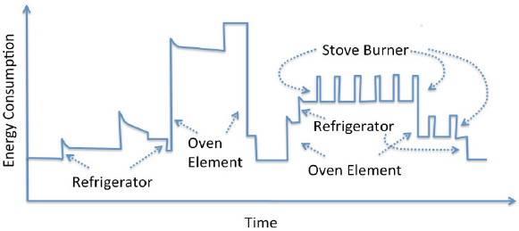
In clustering, a set of entities is given, possibly vectors {x_i}_i, where xi ∈ R^p, and the goal is to assign each of these points to an integer representing its cluster label. Since there are no ground truth labels for clustering, there are many different viable methods for measuring the quality of a clustering. One application of clustering for the power grid is energy disaggregation and nonintrusive load monitoring. The goal of energy disaggregation is to take a single power consumption signal (for instance from a house) and break it into usage by the various appliances (Sultanem, 1991; Hart, 1992). Figure 4.1 illustrates the energy consumption over time of a single household, where there are several appliances contributing to the overall consumption. One can see that each appliance has a unique signature—for instance, the stove burners have short repetitive cycles. Knowledge of detailed energy usage allows (and encourages) consumers to better conserve energy (Darby, 2006; Neenan and Robinson, 2009; Armel et al., 2012).

There are many variations of the energy disaggregation problem (Ziefman and Roth, 2011), but clustering is a key step in several established algorithms (Hart, 1992). The data are whole-house power consumption signals, which can be written as two time series: one for real power, real(t), and one for reactive power, reactive(t), both of which can be calculated from current and voltage signals. Edge detection filters of the form f_j [real(t − Δ), real(t + Δ)] are used to sense different types of changes in the real and reactive power levels, where each j is different. Edge detectors can be useful in finding, for instance, on and off cycles of a dishwasher or a clothes washing machine. Each signal is then represented as a vector of its f_j values. Cluster analysis is then useful for determining which edge signals belong to the same appliances. There are many cases in which data alone do not suffice to build realistic models; domain knowledge can often be used to build realistic structure into the model. The field of reliability engineering exemplifies this (see, for instance, Trivedi, 2001).

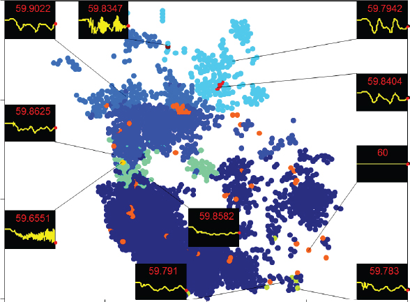
Another use of clustering in the power grid is for visualization and feature extraction from large data sets (Dutta and Overbye, 2014). As an example, Figure 4.2 takes the time-domain bus frequency responses for 16,000 buses from a transient stability study, much as Figure 1.21 showed a time-domain frequency response for generators and then used clustering to group the frequency responses of the buses, showing the results in their geographic context. In the figure the circles correspond to the geographic location of the buses, with the color used to show the buses with a similar response. Sparklines show the average frequency response for each cluster. With this approach the aggregate behavior is apparent, along with identification of the small number of outlier buses.

Reliability Modeling with Physical Models

If a model of how the physical parts of mechanical equipment interact can be created, it can be used to estimate failure probabilities or time until failure. Consider an interconnected network of equipment. Each piece of equipment is represented by a random variable characterizing its hazard rate. This rate depends on neighboring equipment in the network and whether any of them has failed; in that sense, the model is Markovian. One can fit the parameters of this model to data if they are available. In the case of the power network, each piece of equipment on the power grid (substations, transformers, wind turbines, consumers) and their influence on one another would be modeled.

If the equipment has a combinatorial structure (there are components of components, or a logical structure for how one component causes another specific component to fail), this structure can be formalized into reliability block diagrams, reliability graphs, or fault trees, which are specific types of models that govern how components interact and how failures occur in the system. If one does not want to make many assumptions about the components

of the equipment, Markov models of a more general form can also be used for a more data-driven approach, but possibly at the cost of a much larger set of parameters to estimate. Because these physical models completely characterize the physical system, they would allow estimates to be made about failures even when none have ever occurred; updated with data, these models become more powerful.

Cascading Failures

Analysis of the risk posed by cascading failures is a challenging problem that spans several scientific disciplines. At one end the determination of which contingencies (or, perhaps, multiple contingencies) could cause a dangerous cascade must be faced. A large-scale power system example of a cascading failure is the August 14, 2003, Northeast blackout that affected an estimate 50 million people with total costs estimated between $4 billion and $10 billion (U.S.-Canada Power System Outage Task Force, 2004).

The traditional methodology is to enumerate all possibilities of multiple element contingencies, where an individual element could be a transmission line, transformer, or generator. Let k denote the number of simultaneous element outages being considered. As introduced in Chapter 3, N – k contingency analysis seeks to determine whether there are sets with k or fewer elements that when simultaneously taken out of service could cause a cascade. This approach is computationally very expensive even for small values of k. Moreover, it may be too conservative to insist that a system endure any such k contingencies. On the other hand, this criterion may not capture complex network conditions (such as extreme weather), which can impinge on grid operation by triggering multiple contingencies at the same time.

Estimating the consequences of possible multiple contingencies and cascades could prevent those that would be most dangerous. Resources can then be concentrated on measures for preventing those judged to have the highest risk. Comprehensive analyses attempt to predict the behavior of a cascade. This is an especially complex undertaking because it takes place on multiple time scales. Phenomena such as generator tripping are subsecond events, whereas unintentional line tripping may require several minutes. Moreover, both phenomena are subject to noise and unpredictable exogenous elements such as human error and environmental influence. Race conditions between discrete events (when two events are almost simultaneous but it is necessary to determine which actually occurred first) may also need to be modeled to determine the order in which discrete events will occur. These events should be modeled as stochastic events with probability distributions associated with different levels of severity.

Data Assimilation

Dynamical models have states and parameters that must be estimated to perform simulations. Methods for performing these estimations have been extensively developed for linear systems and have become part of standard engineering practice. Data assimilation (DA) extends these methods to incorporate data from observational measurements into model predictions or estimations of states of an ongoing predictive simulation. DA has been used most extensively in weather prediction, where current and recent observations are used to recalibrate the state of large operational forecast models. The key point is that two sources of information are balanced to produce an optimal estimate. There is assumed to be an underlying model that is derived from physical principles and, from the model’s viewpoint, the incorporation of data is accounting for the physics that it is missing. From the viewpoint of the data, the model is providing an extrapolation of the state to times and locations where no measurements are available. This balance between the two types of information, that derived from measurements and that from physical laws, distinguishes data assimilation from other statistical methods such as state estimation, machine learning, and data-driven modeling.

DA is applied in one of two ways: (1) sequentially, in which the state of the system is governed by an evolution equation (the physical model), which is then reinitialized at regular observation times with a new system state that is formed from a systematic interpolation between the state as forecast by the model and the observational data available at that time; and (2) retroactively, where a new state of the system over an entire period of time is estimated as an interpolation between the model state and all available observational data during that period. The former approach is known as sequential DA and the latter as reanalysis. Both approaches rely heavily on ideas

from dynamical systems, and the research at the interface of DA and dynamic stability is particularly active and promising.

There is extraordinary promise in applying DA to issues in the electric grid, because it shares with other areas—namely, weather and climate—where DA has developed a strong underpinning in physical laws combined with considerable observational data. Despite this fact, it seems that DA has had little application, arguably because it is hard to acquire good data that are not proprietary. Nevertheless, its promise as a powerful tool indicates that efforts to develop it for grid models will be bear significant fruit. This can be achieved using partial, available, and/or synthetic data. The fundamental questions can be addressed using data that mimic the actual grid data.

In DA generally, the issues that are receiving most attention are related to the natural tension that occurs between nonlinearity and dimension. In weather and climate modeling, dimensions of the state space are particularly large and growing larger with increasing computational capacity because they are primarily determined by the resolution of the computational model being used. Methods of DA that are effective in these dimensions typically have to make compromises that involve some level of linearization. Nonlinear features of the model can then either be missed or, worse still, cause breakdown of the assimilation process.

The issue of nonlinearity will arise naturally in applying DA in the power system because the underlying equations are highly nonlinear and discontinuous. Indeed, this will be a much more serious issue than in forecasting weather, and the compromises made there may be completely inappropriate for grid predictions and estimates. Moreover, an optimal estimate, as is often sought in DA, will not suffice, because the uncertainties will be as important. A full Bayesian approach would then be necessary, and the issue shifts to whether Gaussian approximations will work.

The ideas of dynamical systems are coming into DA as a way to reduce the dimensions of the necessary calculations. An example is the use of Lyapunov vectors, which capture the most significant unstable directions. With all that is understood about the underlying grid equations as systems of coupled oscillators, this is a particularly promising direction to pursue.

The assimilation of different types of data that are manifest in forms other than state variables is also a challenge to current DA methods. This observational space may play a similar role in determining the dimension reduction. There is considerable structure in the physical model that will both aid and challenge the systematic development of DA strategies. For instance, DA has been mainly developed for large computational models based on fluid dynamics and not for networks. Adapting to this context is, in itself, a challenge and will likely indicate approaches to effective dimension reduction.

COMPLEXITY AND MODEL REDUCTION IN THE TIME OF BIG DATA

Realistic modeling involves large numbers of equations and degrees of freedom improving spatial and temporal resolution of the model, incorporating more physical effects, and describing uncertainty and noise. What is considered “large” in a model has progressed from thousands to tens and even hundreds of millions of variables as computational power has been systematically expanding. Yet there is an unwritten hypothesis of “effective simplicity”—the assumption that an expert is capable of selecting a drastically reduced number of key observables that are sufficient to make useful predictions and to take crucial actions. Model reduction is ubiquitous in applied mathematics: Making a problem as simple as possible, but not simpler, permeates our entire education as modelers. The mathematical underpinnings of model reduction (such as separation of time scales or averaging) have given rise to tools and techniques (quasi-steady-state approximation for reducing chemical kinetics, homogenization for the description of heterogeneous materials) that dramatically affect the ability to simulate, design, control, and rationalize the behavior of complex dynamical systems. Aggregation of degrees of freedom (e.g., of the many loads in a household within a distribution system, or reducing the effects of a distribution system on a transmission network to a single effective degree of freedom), so that coarse-grained, effective grid models can be usefully analyzed, is already common practice.

The ability to systematically derive useful reduced models has traditionally, however, been very restricted: The symbolic computation of, say, center manifolds for dynamical systems, while conceptually powerful, becomes

quickly intractable, and an “expert” is almost by definition someone who can extract meaningful reduced models and the understanding that comes with them from extensive personal experience/wisdom.

High-performance computing, on the one hand, and data mining/machine learning on the other, are gradually (but at an accelerating pace) changing the way this expert knowledge is obtained. Useful reduced models are now increasingly obtained on the fly as a by-product of detailed scientific computation and/or by the mining of resolved computational/observational data. And while the resulting models and computations may not reflect the intuition or experience of human experts, they can be reliably tested and used. It is remarkable that many large-scale scientific computation techniques, from multigrid to preconditioning to Krylov integrator methods, implicitly rely on this online reduction process to successfully accelerate computation.

Instead of searching for reduction in the structure of dynamic models (e.g., looking for fast equilibrating processes so that they can be modeled at quasi-equilibrium and thus reduce the problem size), it is now possible to search for low dimensionality and reduction directly in both observational and simulation data. Principal component analysis held pride of place in data reduction for a hundred years; then, in the 1980s, neural networks briefly held unfulfilled promise before coming back as deep learning today. The manifold learning tools that have arisen in the last two decades (from ISOMAP to locally linear embedding to kernel principal component analysis to diffusion maps and their extensions) have used semidefinite programming relaxations to open a new window in the way effective simplicity can be discovered and algorithmically perform model reduction as a wrapper around detailed simulation codes. Smart precomputation and tabulation techniques, such as in situ adaptive tabulation and intrinsic low-dimensional manifolds, along with the associated fast database search/access, further exploit these new tools to accelerate computation. Instead of trying to derive smart reduced models (that is, deduce/discover the truly important observable quantities and then express the dynamics in terms of these quantities), detailed evolution models are written with the best physics available. These models are used in a sense as computational experiments: Instead of running them for all times, all feasible parameter values, and all reasonable initial conditions, one can run them in brief simulation bursts, process the resulting data to discover online their local useful reduction, and use this information to design the next informative short simulation burst. In effect, one is implementing singular perturbation or averaging techniques computationally rather than symbolically. The mathematics of reduction are the same as when these models can be explicitly performed on formulas, but now the reductions are based on computational observations.

In this spirit, detailed grid simulations can be effectively reduced online so that computations to identify stationary states, stability results, or control designs become tractable. This online reduction in complexity relies first on mining of computational or observational data to discover the right local variable aggregation and then on brief bursts of simulation by the disaggregated simulator to extract new, useful aggregated information. In effect, one solves the reduced model without ever writing it down in closed form and finds the relevant coarse-grained variables without necessarily being able to articulate their description.

This type of effective modeling, which crucially relies on machine learning for the detection of the important observables parameterizing the high-dimensional state data, holds promise for many complex but effectively simple systems models, especially for the power grid. A nontrivial twist arises from the fact that some of the data that one wishes to effectively compress are not just real numbers (components of a vector in Rn for very large n) but are also integers (such as the adjacency matrices defining the connectivities of networks of units). In this case, mining data in the form of networks/graphs rather than just as points in high-dimensional spaces becomes a challenge. What is also a challenge is the issue of comprehensibility to human experts: discovering descriptions that are isomorphic to the mathematically obtained descriptions yet are easily interpretable by humans.

The promise of this approach lies not in better modeling but in smarter, faster, possibly more easily understandable extraction of relevant information from the best written models. One of its main strengths is its “wrapper” philosophy: Since we are wrapping postprocessing algorithms (as accelerators/enablers) around our best simulators, we can still make improvements to those simulators—reflecting our best understanding of physical processes and details of simulator dynamics—and it won’t require changes to the wrapper algorithms. As a matter of fact, part of the original motivation in devising this computational enabling technology was the desire to force legacy codes to perform tasks they were not intrinsically designed to do. As such, these algorithms can be wrapped around existing

validated simulators, and they enhance the speed and reliability of extracting information from the simulations without needing to validate them anew.

UNCERTAINTY QUANTIFICATION

Viewing the power system as a complex, many-degree-of-freedom, nonlinear dynamical system gives rise to a hierarchy of model formulations, each with its own uses in both the design and operation phases. Deterministic steady-state formulations (giving rise to large sets of algebraic equations) and deterministic time-dependent formulations (giving rise to large sets of nonlinear differential, or differential algebraic equations) have been, and continue to be, useful. Still, taking into account and successfully modeling the inherently stochastic nature of the grid operation is increasingly the driver in pushing the boundary of the state of the art both in mathematical modeling and in algorithm development for grid design and operation.

There are aspects of uncertainty that have always been present in grid modeling and cannot be prescribed or measured accurately in advance. The uncertainty of grid loads is ever present, but the uncertainty inherent in renewable energy production, especially in solar panels and wind turbine farms owing to weather variability, poses a new set of challenges. Furthermore, the anticipated real-time interaction of renewable energy generation with energy pricing (especially as storage technology options develop) brings an additional level of complexity.

Fortunately, there is an explosion in the mathematics and computation of uncertainty quantification driven by many different natural, technological, and financial problems (weather prediction being a crucial driver). Once deterministic dynamical systems tools became more mature, uncertainty and stochasticity became the natural research frontier. It might be useful to make a distinction between uncertain parameters (unknown fixed values, for which a distribution is known, estimated, or postulated) and uncertain, time-dependent processes. For uncertain parameters, techniques based on Wiener’s polynomial chaos (PC) expansion—expanding the uncertain solution of a given problem as a function of the uncertain parameter(s), using as basis functions orthogonal polynomials constructed from the parameter uncertainty distribution—have experienced a broad resurgence over the last two decades. Used for linear uncertain problems for many years (especially in civil engineering), the approach is now being used in nonlinear problems across many sciences. It has been implemented in publicly available software and has driven important numerical developments in the use of sparse (Smolyak) grids in what are called nonintrusive computational methods, circumventing the stochastic Galerkin approximation through high-dimensional collocation. Indeed, if the distributions of uncertainty of different parameters are independent, then a relatively large number (O(100)) of uncertain parameters can be practically modeled. Such Wiener PC tools can also be used in the case of uncertain processes (e.g., in stochastic partial differential equation with Brownian motion forcing). Alternative approaches, such as analysis of variance techniques (including adaptive ones) and the optimal uncertainty quantification framework, are being developed and find applications in the context of the power system (e.g., in quantifying uncertainty for large-scale dynamic simulations of power systems).

It is crucial to recognize, however, that the number of uncertain parameters/stochastic variables that enter modern power system models is, and will remain, beyond what one can usefully compute, and that therefore reduction techniques (and, importantly, data-driven reduction techniques as well as state estimation and particle filtering techniques) will play an important role in making computational uncertainty quantification sufficiently manageable as to be practically useful. This will involve building smart reduced parameterizations of uncertainty in dynamic models, and methods for estimating probability density functions or covariance matrices for the forcing terms in the models based on finite measurements—a context where, for example, multidimensional Gaussian processes and Bayesian approaches become relevant.

But while parameterizing uncertainty in a model (both for the inputs, and the loads, and the outputs) is crucial, it is only the first step necessary for formulating the problem. The most important component is the development of simulation/optimization algorithms that will actually solve the problem (plan energy production and decide dynamically on net interchange schedules and allocations). These will operate at the hardware design level (constituting the network, building in the reconfigurability/safeguard capabilities that will guarantee safe/acceptable/optimal operation) and also, more challengingly, at the day-to-day and hour-to-hour operation planning level.

The computational scalability of stochastically optimizing the design and operation of complex energy systems is an important frontier; usefully decomposing stochastic optimization problems on a scenario basis and successfully distributing scenarios/sampling strategies over processors hold promise for solving, for example, stochastic economic dispatch problems that use hourly wind forecasts to integrate wind power with the real-time energy market.

Ultimately, the biggest challenge will be at the confluence of power system hardware, renewable energy production uncertainty, and interactions with real-time prices as renewable energy production becomes more and more integrated in the grid. The relation between, say, day-ahead and expected real-time prices, and the ways this may bias economic incentives, induces an additional uncertainty quantification/uncertainty propagation layer that makes large-scale problems simply unsolvable today.

REFERENCES

Kuznetsov, Y.A. 2004. Numerical Analysis of Bifurcations. Springer, New York.

Linderoth, J.T., A. Shapiro, and S.J. Wright. 2006. The empirical behavior of sampling methods for stochastic programming. Annals of Operations Research 142:219-245.

Low, S. 2014. Convex relaxation of optimal power flow, Part I: Formulations and equivalence. IEEE Transactions on Control of Network Systems 1(1):15-27.

Martinussen, T., and T.H. Scheike. 2006. Dynamic Regression Models for Survival Data. Springer, New York, N.Y.

NASPI. 2015. NASPI 2014 Survey of Synchrophasor System Networks—Results and Findings. Technical report. Data and Network Management Task Team, Network Systems Group. July. https://www.naspi.org/documents.

Neenan, B., and J. Robinson. 2009. Residential Electricity Use Feedback: A Research Synthesis and Economic Framework. Technical report. Electric Power Research Institute.

Nemhauser, G.L., and L.A. Wolsey. 1998. Integer and Combinatorial Optimization. Wiley, New York, N.Y.

Nocedal, J., and S. Wright. 2006. Numerical Optimization, 2nd ed. Springer.

Oliveira, W., C. Sagastizbal, and S. Scheimberg. 2011. Inexact bundle methods for two-stage stochastic programming. SIAM Journal on Optimization 21:517-544.

Papavasiliou, A. and S.S. Oren. 2013. A comparative study of stochastic unit commitment and security-constrained unit commitment using high performance computing. Proceedings of the 2013 European Control Conference (ECC), pp. 2507-2512.

PJM. 2014. Load Forecasting and Analysis, Manual 19, Revision 26. Effective date November 1. Prepared by Resource Adequacy Planning.

Prékopa, A. 1995. Stochastic Programming. Kluwer.

Rockafellar, R.T. 1993. Lagrange multipliers and optimality. SIAM Review 35(2):183-238.

Schrijver, A. 1998. Theory of Linear and Integer Programming. Wiley, London, U.K.

Shapiro, A., D. Dentcheva, and A. Ruszczyński. 2009. Lectures on Stochastic Programming: Modeling and Theory. MOS-SIAM Series on Optimization. Society for Industrial and Applied Mathematics. http://dx.doi.org/10.1137/1.9780898718751.

Sheble, G.B., and G.N. Fahd. 1994. Unit commitment literature synopsis. IEEE Transactions on Power Systems 9(1):128-135.

Shiina, T., and J.R. Birge. 2004. Stochastic unit commitment problem. International Transactions in Operational Research 11:19-32.

Soliman, S., and A. Kandari. 2010. Electrical Load Forecasting: Modeling and Model Construction. Elsevier. ISBN 978-0-12-381543-9.

Sultanem, F. 1991. Using appliance signatures for monitoring residential loads at meter panel level. IEEE Transaction on Power Delivery 6(4):1380-1385.

Trivedi, K. 2001. Probability and Statistics with Reliability, Queueing, and Computer Science Applications, 2nd ed. Wiley, New York, N.Y.

U.S.-Canada Power System Outage Task Force. 2004. Final Report on the August 14, 2003 Blackout in the United States and Canada: Causes and Recommendations. April. http://www.nerc.com/docs/docs/blackout/ch1-3.pdf.

Van Slyke, R., and R. J-B. Wets. 1969. L-shaped linear programs with application to optimal control and stochastic programming. SIAM Journal of Applied Mathematics 17:638–663.

Wang, Q., Y. Guan, and J. Wang. 2012. A chance-constrained two-stage stochastic program for unit commitment with uncertain wind power output. IEEE Transactions on Power Systems 27:206-215.

Wehenkel, L.A. 1998. Automatic Learning Techniques in Power Systems. Kluwer International Series in Engineering and Computer Science. Kluwer Academic Publishers, Norwell, Mass.

Wischkaemper, J.A., C.L. Benner, B.D. Russell, and K.M. Manivannan. 2014. “Waveform Analytics-based Improvements in Situational Awareness, Feeder, Visibility, and Operational Efficiency,” Proceedings of the 2014 IEEE PES T&D Conference and Exposition. doi:10.1109/ TDC.2014.6863349.

Wischkaemper, J.A., C.L. Benner, B.D. Russell, and K. Manivannan. 2015. Application of waveform analytics for improved situational awareness of electric distribution feeders. IEEE Transactions on Smart Grid 6(4):2041-2049.

Wolsey, L.A. 1998. Integer Programming. Wiley, New York, N.Y.

Zeifman, M., and K. Roth. 2011. Nonintrusive appliance load monitoring: Review and outlook. IEEE Transactions on Consumer Electronics 57(1):76-84.

REFERENCES

Andersson, G. 2004. Modelling and Analysis of Electric Power Systems. Power Systems Laboratory, ETH, Zurich. March.
Armel, K.C., A. Gupta, G. Shrimali, and A. Albert. 2012. “Is Disaggregation the Holy Grail of Energy Efficiency? The Case of Electricity.” Technical Paper Series: PTP-2012-05-1. Precourt Energy Efficiency Center, Stanford University, Calif. Published in 2013 in Energy Policy 52(C):213-234.
Bard, J.F., and J.T. Moore. 1990. A branch and bound algorithm for the bilevel programming problem. SIAM Journal on Scientific and Statistical Computing 11(2):281-292.
Belotti, P., C. Kirches, S. Leyffer, J. Linderoth, J. Luedtke, and A. Mahajan. 2013. Mixed-integer nonlinear optimization. Acta Numerica 22:1-131.
Benders, J.F. 1962. Partitioning procedures for solving mixed-variables programming problems. Numerische Mathematik, 4:238–252.
Ben-Tal, R., and A. Nemirovski. 2000. Robust solutions of linear programming problems contaminated with uncertain data. Mathematical Programming 88:411-424.
Bertsimas, D., D.B. Brown, and C. Caramanis. 2011. Theory and applications of robust optimization. SIAM Review 53(3):464-501.
Bienstock, D. 2013. Progress on solving power flow problems. Optima Mathematical Optimization Society Newsletter 93:1-7.
Bienstock, D., M. Chertkov, and S. Harnett. 2014. Chance-constrained optimal power flow: Risk aware network control under uncertainty. SIAM Review 56(3):461-495.
Birge, J.R., and F. Louveaux. 2011. Introduction to Stochastic Programming. Springer Series in Operations Research and Financial Engineering. Springer-Verlag, New York, N.Y.
Bixby, R.E. 2015. “Mixed-Integer Programming: It Works Better Than You May Think.” Presentation to the National Research Council workshop Analytical Research Foundations for the Next-Generation Electric Grid on February 11-12, 2015, in Irvine, Calif.
Cain, M., R.P. O’Neill, and A. Castillo. 2013. History of optimal power flow and formulations, Optimal power flow paper 1. Federal Regulatory Commission.
Castillo, A. and R.P. O’Neill. 2013a. Survey of approaches to solving the ACOPF, Optimal power flow paper 4. Federal Regulatory Commission.
Castillo, A. and R.P. O’Neill. 2013b. Computational performance of solution techniques applied to the ACOPF, Optimal power flow paper 5. Federal Regulatory Commission.
Darby, S. 2006. The Effectiveness of Feedback on Energy Consumption. A Review for DEFRA of the Literature on Metering, Billing, and Direct Displays. Technical report. Environmental Change Institute, University of Oxford. April.
Dobson, I. 1992. Observations on the geometry of saddle node bifurcation and voltage collapse in electrical power systems. IEEE Transactions on Circuits and Systems I: Fundamental Theory and Applications 39(3).
Dutta, S., and T.J. Overbye. 2014. Feature extraction and visualization of power system transient stability results. IEEE Transactions on Power Systems 29(2):966-973.
Ferris, M.C., Z. Friedman, D. Molzahn, C. DeMarco, and B. Lesieutre. ACOPF models: Extending data, formulations, and solution methodology, presentation given June 2013. See http://pages.cs.wisc.edu/~ferris/talks/ferc-jun.pdf. Accessed December 1, 2015.
Goldberg, M. 2015. Presentation to the National Research Council Workshop on Analytical Research Foundations for the Next-Generation Electric Grid in February in Irvine, Calif.
Glover, J.D., M.S. Sarma, and T.J. Overbye. 2012. Power System Analysis and Design, Fifth Edition. Cengage Learning.
Guckenheimer, J., and P. Holmes. 1983. Nonlinear Oscillations, Dynamical Systems, and Bifurcations of Vector Fields (Applied Mathematical Sciences), 1st ed. Springer-Verlag, New York, N. Y.
Hairer, E., and G. Wanner. 2004. Solving Ordinary Differential Equations (I). Springer-Verlag, New York, N. Y.
Hairer, E., and G. Wanner. 2009. Solving Ordinary Differential Equations (II). Springer-Verlag, New York, N. Y.
Hart, G. 1992. Nonintrusive appliance load monitoring. Proceedings of the IEEE 80(12):1870-18912.
Hedman, K.W., S.S. Oren, and R.P. O’Neill. 2011. “A Review of Transmission Switching and Network Topology Optimization.” IEEE PES General Meeting, Detroit.
Heidel, T. 2014. “Advanced Research Projects Agency-Energy,” Grid Optimization Workshop Introduction. Presentation to the Advanced Bulk Power System Optimization Technologies Workshop on November 13-14, 2014, U.S. Department of Energy, http://arpa-e.energy.gov/?q=workshop/advanced-bulk-power-system-optimization-technologies-workshop.
Higle, J.L., and S. Sen. 1991. Stochastic decomposition: An algorithm for two-stage linear programs with recourse. Mathematics of Operations Research 16:650-669.