Guide for Pavement Friction (2009)

Below is the uncorrected machine-read text of this chapter, intended to provide our own search engines and external engines with highly rich, chapter-representative searchable text of each book. Because it is UNCORRECTED material, please consider the following text as a useful but insufficient proxy for the authoritative book pages.

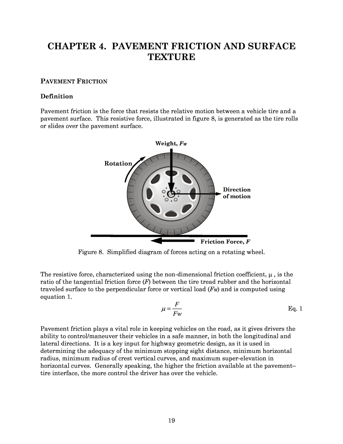
19 CHAPTER 4. PAVEMENT FRICTION AND SURFACE TEXTURE PAVEMENT FRICTION Definition Pavement friction is the force that resists the relative motion between a vehicle tire and a pavement surface. This resistive force, illustrated in figure 8, is generated as the tire rolls or slides over the pavement surface. Figure 8. Simplified diagram of forces acting on a rotating wheel. The resistive force, characterized using the non-dimensional friction coefficient, μ , is the ratio of the tangential friction force (F) between the tire tread rubber and the horizontal traveled surface to the perpendicular force or vertical load (FW) and is computed using equation 1. Fw F=μ Eq. 1 Pavement friction plays a vital role in keeping vehicles on the road, as it gives drivers the ability to control/maneuver their vehicles in a safe manner, in both the longitudinal and lateral directions. It is a key input for highway geometric design, as it is used in determining the adequacy of the minimum stopping sight distance, minimum horizontal radius, minimum radius of crest vertical curves, and maximum super-elevation in horizontal curves. Generally speaking, the higher the friction available at the pavement– tire interface, the more control the driver has over the vehicle. Weight, FW Friction Force, F Direction of motion Rotation

20 Longitudinal Frictional Forces Longitudinal frictional forces occur between a rolling pneumatic tire (in the longitudinal direction) and the road surface when operating in the free rolling or constant-braked mode. In the free-rolling mode (no braking), the relative speed between the tire circumference and the pavement—referred to as the slip speed—is zero. In the constant-braked mode, the slip speed increases from zero to a potential maximum of the speed of the vehicle. The following mathematical relationship explains slip speed (Meyer, 1982): Eq. 2 where: S = Slip speed, mi/hr. V = Vehicle speed, mi/hr. VP = Average peripheral speed of the tire, mi/hr. ω = Angular velocity of the tire, radians/sec. r = Average radius of the tire, ft. Again, during the free-rolling state of the tire, VP is equal to the vehicle speed; thus, S is zero. For a locked or fully braked wheel, VP is zero, so the sliding speed or slip speed is equal to the vehicle speed (V). A locked-wheel state is often referred to as a 100 percent slip ratio, and the free-rolling state is a zero percent slip ratio. The following mathematical relationships give the calculation formula for slip ratio (Meyer, 1982): Eq. 3 where: SR = Slip ratio, percent. V = Vehicle speed, mi/hr. VP = Average peripheral speed of the tire, mi/hr. S = Slip speed, mi/hr. Similar to the previous explanation, during the free-rolling state of the tire, VP is equal to the vehicle speed and S is zero, thus the slip ratio (SR) is zero percent. For a locked wheel, VP is zero, S equals the vehicle speed (V), and so the slip ratio (SR) is 100 percent. Figure 9 shows the ground force acting on a free rolling tire. In this mode, the ground force is at the center of pressure of the tire contact area and is off center by the amount a. This offset causes a moment that must be overcome to rotate the tire. The force required to counter this moment is called the rolling resistance force (FR). The value a is a function of speed and increases with speed. Thus, FR increases with speed. In the constant-braked mode (figure 10), an additional force called the braking slip force (FB) is required to counter the added moment (MB) created by braking. The force is proportional to the level of braking and the resulting slip ratio. The total frictional force is the sum of the free-rolling resistance force (FR) and the braking slip force (FB). )68.0( rVVVS P ××−=−= ω 100100 ×=×−= V S V VVSR P

21 Figure 9. Rolling resistance force with a free-rolling tire at a constant speed on a bare, dry paved surface (Andresen and Wambold, 1999). Figure 10. Forces and moments of a constant-braked wheel on a bare, dry paved surface (Andresen and Wambold, 1999). a Ground Force, FG Free body diagram, steady state Weight, FW Radius, r Rotation Direction of Motion Rolling Resistance Force, FR Braking Moment, MB Braking Slip Force, FB a Ground Force, FG Free body diagram, steady state Weight, FW Radius, r Rotation Direction of Motion Rolling Resistance Force, FR

22 The coefficient of friction between a tire and the pavement changes with varying slip, as shown in figure 11 (Henry, 2000). The coefficient of friction increases rapidly with increasing slip to a peak value that usually occurs between 10 and 20 percent slip (critical slip). The friction then decreases to a value known as the coefficient of sliding friction, which occurs at 100 percent slip. The difference between the peak and sliding coefficients of friction may equal up to 50 percent of the sliding value, and is much greater on wet pavements than on dry pavements. The relationship shown in figure 11 is the basis for the anti-locking brake system (ABS), which takes advantage of the front side of peak friction and minimizes the loss of side/steering friction due to sliding action. Vehicles with ABS are designed to apply the brakes on and off (i.e., pump the brakes) repeatedly, such that the slip is held near the peak. The braking is turned off before the peak is reached and turned on at a set time or percent slip below the peak. The actual timing is a proprietary design of the manufacturer. Figure 11. Pavement friction versus tire slip. Lateral Frictional Forces Another important aspect of friction relates to the lateral or side-force friction that occurs as a vehicle changes direction or compensates for pavement cross-slope and/or cross wind effects. The relationship between the forces acting on the vehicle tire and the pavement surface as the vehicle steers around a curve, changes lanes, or compensates for lateral forces is as follows: Eq. 4 Peak friction Critical slip Full sliding 100 (fully-locked) 0 (free rolling) Tire Slip, % Coefficient of Friction Increased Braking Intermittent sliding e R VFS −= 15 2

23 where: FS = Side friction. V = Vehicle speed, mi/hr. R = Radius of the path of the vehicle’s center of gravity (also, the radius of curvature in a curve), ft. e = Pavement super-elevation, ft/ft. This equation is based on the pavement–tire steering/cornering force diagram in figure 12. It shows how the side-force friction factor acts as a counterbalance to the centripetal force developed as a vehicle performs a lateral movement. Figure 12. Dynamics of a vehicle traveling around a constant radius curve at a constant speed, and the forces acting on the rotating wheel. Combined Braking and Cornering With combined braking and cornering, a driver either risks not stopping as rapidly or losing control due to reduced lateral/side forces. When operating at the limits of tire grip, the interaction of the longitudinal and lateral forces is such that as one force increases, the other must decrease by a proportional amount. The application of longitudinal braking reduces the lateral force significantly. Similarly, the application of high lateral force reduces the longitudinal braking. Figure 13 shows these effects (Gillespie, 1992). Commonly referred to as the friction circle or friction ellipse (Radt and Milliken, 1960), the vector sum of the two combined forces remains constant (circle) or near constant (ellipse) (see figure 14). When operating within the limits of tire grip, the amount of braking and turning friction components can vary independently as long as the vector sum of these components does not exceed the limits of tire grip as defined by the friction circle or friction ellipse. The degree of ellipse depends on the tire and pavement properties. W Weight of vehicle P Centripetal force (horizontal) FS Friction force between tires and roadway surface (parallel to roadway surface) α Angle of super-elevation (tan α = e) R Radius of curve α α W P FS Direction of Travel Drag Force Side Friction Force (Friction Factor) Friction Measuring Wheel

24 Figure 13. Brake (Fx) and lateral (Fy) forces as a function of longitudinal slip (Gillespie, 1992). Figure 14. Lateral force versus longitudinal force at constant slip angles (Gillespie, 1992). Friction Mechanisms Pavement friction is the result of a complex interplay between two principal frictional force components—adhesion and hysteresis (figure 15). Adhesion is the friction that results from the small-scale bonding/interlocking of the vehicle tire rubber and the pavement surface as they come into contact with each other. It is a function of the interface shear strength and contact area. The hysteresis component of frictional forces results from the energy loss due

25 Figure 15. Key mechanisms of pavement–tire friction. to bulk deformation of the vehicle tire. The deformation is commonly referred to as enveloping of the tire around the texture. When a tire compresses against the pavement surface, the stress distribution causes the deformation energy to be stored within the rubber. As the tire relaxes, part of the stored energy is recovered, while the other part is lost in the form of heat (hysteresis), which is irreversible. That loss leaves a net frictional force to help stop the forward motion. Although there are other components of pavement friction (e.g., tire rubber shear), they are insignificant when compared to the adhesion and hysteresis force components. Thus, friction can be viewed as the sum of the adhesion and hysteresis frictional forces. Eq. 5 Both components depend largely on pavement surface characteristics, the contact between tire and pavement, and the properties of the tire. Also, because tire rubber is a visco-elastic material, temperature and sliding speed affect both components. Because adhesion force is developed at the pavement–tire interface, it is most responsive to the micro-level asperities (micro-texture) of the aggregate particles contained in the pavement surface. In contrast, the hysteresis force developed within the tire is most responsive to the macro-level asperities (macro-texture) formed in the surface via mix design and/or construction techniques. As a result of this phenomenon, adhesion governs the overall friction on smooth-textured and dry pavements, while hysteresis is the dominant component on wet and rough-textured pavements. Hysteresis Depends mostly on macro- level surface roughness Adhesion Depends mostly on micro-level surface roughness Rubber Element V F HA FFF +=

26 Factors Affecting Available Pavement Friction The factors that influence pavement friction forces can be grouped into four categories— pavement surface characteristics, vehicle operational parameters, tire properties, and environmental factors. Table 2 lists the various factors comprising each category. Because each factor in this table plays a role in defining pavement friction, friction must be viewed as a process instead of an inherent property of the pavement. It is only when all these factors are fully specified that friction takes on a definite value. The more critical factors are shown in bold in table 2 and are briefly discussed below. Among these factors, the ones considered to be within a highway agency’s control are micro- texture and macro-texture, pavement materials properties, and slip speed. Table 2. Factors affecting available pavement friction (modified from Wallman and Astrom, 2001). Pavement Surface Characteristics Vehicle Operating Parameters Tire Properties Environment • Micro-texture • Macro-texture • Mega-texture/ unevenness • Material properties • Temperature • Slip speed ¾ Vehicle speed ¾ Braking action • Driving maneuver ¾ Turning ¾ Overtaking • Foot Print • Tread design and condition • Rubber composition and hardness • Inflation pressure • Load • Temperature • Climate ¾ Wind ¾ Temperature ¾ Water (rainfall, condensation) ¾ Snow and Ice • Contaminants ¾ Anti-skid material (salt, sand) ¾ Dirt, mud, debris Note: Critical factors are shown in bold. Pavement Surface Characteristics Surface Texture Pavement surface texture is characterized by the asperities present in a pavement surface. Such asperities may range from the micro-level roughness contained in individual aggregate particles to a span of unevenness stretching several feet in length. The two levels of texture that predominantly affect friction are micro-texture and macro-texture (Henry, 2000). As figure 16 shows, micro-texture is the degree of roughness imparted by individual aggregate particles, whereas macro-texture is the degree of roughness imparted by the deviations among particles. Micro-texture is mainly responsible for pavement friction at low speeds, whereas macro-texture is mainly responsible for reducing the potential for separation of tire and pavement surface due to hydroplaning and for inducing friction caused by hysteresis for vehicles traveling at high speeds. Further discussions on micro- texture and macro-texture are provided later in this chapter under the heading “Pavement Surface Texture.”

27 Figure 16. Micro-texture versus macro-texture (Flintsch et al., 2003). Surface Material Properties Pavement surface material properties (i.e., aggregate and mix characteristics, texturing patterns) help to define surface texture. These properties also affect the long-term durability of texture through their capacities to resist aggregate polishing and abrasion/wear of both aggregate and mix under accumulated traffic and environmental loadings. Vehicle Operating Parameters Slip Speed The coefficient of friction between a tire and the pavement changes with varying slip. It increases rapidly with increasing slip to a peak value that usually occurs between 10 and 20 percent slip. The friction then decreases to a value known as the coefficient of sliding friction, which occurs at 100 percent slip. Tire Properties Tire Tread Design and Condition Tire tread design (i.e., type, pattern, and depth) and condition have a significant influence on draining water that accumulates at the pavement surface. Water trapped between the pavement and the tire can be expelled through the channels provided by the pavement surface texture and by the tire tread. The depth of tread is particularly important for vehicles driving over thick films of water at high speeds. Some studies (Henry, 1983) have reported a decrease in wet friction of 45 to 70 percent for fully worn tires, compared to new ones. Tire Inflation Pressure Tire under-inflation can significantly reduce friction at high speeds. Under-inflated tires allow the center of the tire tread to collapse and become very concave, resulting in the constriction of drainage channels within the tire tread and a reduction of contact pressure.

28 The effect is for the tire to trap water at the pavement surface rather than allow it to flow through the treads. As a consequence, hydroplaning speed is decreased. Tire over-inflation, on the other hand, causes only a small loss of pavement friction (Henry, 1983; Kulakowski et al., 1990). Over-inflated tires reduce the trapping effect and yield higher pressure for forcing water from below the vehicle’s tire. The increased tire pressure and smaller tire contact area result in a higher hydroplaning speed. Environment Thermal Properties Automotive tires are visco-elastic materials, and their properties can be significantly affected by changes in temperature and other thermal properties, such as thermal conductivity and specific heat. Research indicates that pavement–tire friction generally decreases with increasing tire temperature, though this is difficult to quantify. Water Water, in the form of rainfall or condensation, can act as a lubricant, significantly reducing the friction between tire and pavement. The effect of water film thickness (WFT) on friction is minimal at low speeds (<20 mi/hr [32 km/hr]) and quite pronounced at higher speeds (>40 mi/hr [64 km/hr]). As shown in figure 17, the coefficient of friction of a vehicle tire sliding over a wet pavement surface decreases exponentially as WFT increases. The rate at which the coefficient of friction decreases generally becomes smaller as WFT increases. In addition, the effect of WFT is influenced by tire design and condition, with worn tires being most sensitive to WFT. Figure 17. Effect of water film thickness on pavement friction (Henry, 2000). WFT, in Fr ic ti on 0 0.005 0.01 0.015 0.02 0.025 0.03 0.035 25 30 35 40 45 50 Worn Ribbed Tire New Ribbed Tire Smooth Tire

29 A very small amount of water can significantly reduce pavement friction. Test results from an FHWA-sponsored study (Harwood, 1987) indicate that as little as 0.002 in (0.05 mm) of water on the pavement surface can reduce the coefficient of friction by 20 to 30 percent of the dry coefficient of friction. In some cases, a 0.001-in (0.025-mm) water film can reduce friction significantly. Such a thin film is likely to form during any hour in which at least 0.01 in (0.25 mm) of rain has fallen. Hydroplaning can occur when relatively thick water layers or films are present and vehicles are traveling at higher speeds. Hydroplaning occurs when a vehicle tire is separated from the pavement surface by the water pressure that builds up at the pavement–tire interface (Horne and Buhlmann, 1983), causing friction to drop to a near-zero level. It is a complex phenomenon affected by several parameters, including water depth, vehicle speed, pavement macro-texture, tire tread depth, tire inflation pressure, and tire contact area. Relatively thick water films form on a pavement surface when drainage is inadequate during heavy rainfalls or when pavement rutting or wearing creates puddles. Loss of direct pavement–tire contact can occur at speeds as low as 40 to 45 mi/hr (64 to 72 km/hr) on puddles about 1 in (25 mm) deep and 30 ft (9 m) long (Hayes et al., 1983). Pavement macro-texture and tire tread depth influence the onset of dynamic hydroplaning in two ways. First, they have a direct effect on the critical hydroplaning speed because they provide a pathway for water to escape from the pavement–tire interface. Second, they have an indirect effect on the critical hydroplaning speed since the larger the macro-texture, the deeper the water must be to cause hydroplaning. However, the pavement surface must also have the proper micro-texture to develop adequate friction. Snow and Ice Snow and ice on the pavement surface present the most hazardous condition for vehicle braking or cornering. The level of friction between the tires and the pavement is such that almost any abrupt braking or sudden change of direction results in locked-wheel sliding and loss of vehicle directional stability. NCHRP Web Document 53 (Al Qadi et al., 2002) noted that vehicle friction performance can be drastically degraded if the tire contact area does not reach the pavement surface because of ice and snow. Contaminants Contaminants commonly found on highways include dirt, sand, oil, water, snow, and ice. Any kind of contamination at the pavement–tire interface will have an adverse effect on pavement–tire friction. Foreign materials act like the balls in a ball bearing, or as lubricant between a piston and cylinder in an engine, reducing friction between the two surfaces. The thicker or more viscous the contaminant, the greater the reduction in pavement–tire friction. The grinding effect of hard contaminants, such as sand, accelerates the rate of wearing at the pavement surface.

30 PAVEMENT SURFACE TEXTURE Definition Pavement surface texture is defined as the deviations of the pavement surface from a true planar surface. These deviations occur at three distinct levels of scale, each defined by the wavelength (λ) and peak-to-peak amplitude (A) of its components. The three levels of texture, as established in 1987 by the Permanent International Association of Road Congresses (PIARC), are as follows: • Micro-texture (λ < 0.02 in [0.5 mm], A = 0.04 to 20 mils [1 to 500 µm])—Surface roughness quality at the sub-visible or microscopic level. It is a function of the surface properties of the aggregate particles contained in the asphalt or concrete paving material. • Macro-texture (λ = 0.02 to 2 in [0.5 to 50 mm], A = 0.005 to 0.8 in [0.1 to 20 mm])— Surface roughness quality defined by the mixture properties (shape, size, and gradation of aggregate) of asphalt paving mixtures and the method of finishing/texturing (dragging, tining, grooving; depth, width, spacing and orientation of channels/grooves) used on a concrete paved surfaces. • Mega-texture (λ = 2 to 20 in [50 to 500 mm], A = 0.005 to 2 in [0.1 to 50 mm])— Texture with wavelengths in the same order of size as the pavement–tire interface. It is largely defined by the distress, defects, or “waviness” on the pavement surface. Wavelengths longer than the upper limit (20 in [500 mm]) of mega-texture are defined as roughness or unevenness (Henry, 2000). Figure 18 illustrates the three texture ranges, as well as a fourth level—roughness/unevenness—representing wavelengths longer than the upper limit (20 in [500 mm]) of mega-texture. It is widely recognized that pavement surface texture influences many different pavement– tire interactions. Figure 19 shows the ranges of texture wavelengths affecting various vehicle–road interactions, including friction, interior and exterior noise, splash and spray, rolling resistance, and tire wear. As can be seen, friction is primarily affected by micro- texture and macro-texture, which correspond to the adhesion and hysteresis friction components, respectively. Figure 20 shows the relative influences of micro-texture, macro-texture, and speed on pavement friction. As can be seen, micro-texture influences the magnitude of tire friction, while macro-texture impacts the friction–speed gradient. At low speeds, micro-texture dominates the wet and dry friction level. At higher speeds, the presence of high macro- texture facilitates the drainage of water so that the adhesive component of friction afforded by micro-texture is re-established by being above the water. Hysteresis increases with speed exponentially, and at speeds above 65 mi/hr (105 km/hr) accounts for over 95 percent of the friction (PIARC, 1987).

31 Figure 18. Simplified illustration of the various texture ranges that exist for a given pavement surface (Sandburg, 1998). Figure 19. Texture wavelength influence on pavement–tire interactions (adapted from Henry, 2000 and Sandburg and Ejsmont, 2002). Roughness/Unevenness Reference Length Short stretch of road Tire Mega-texture Amplification ca. 50 times Amplification ca. 5 times Amplification ca. 5 times Road–Tire Contact Area Macro-texture Micro-texture Single Chipping 10-6 10-5 10-4 10-3 10-2 10-1 100 101 m Micro-texture Macro-texture Mega-texture Roughness/Unevenness Int. Noise Splash/Spray Rolling Resistance Tire/Vehicle Damage Texture Wavelength Note: Darker shading indicates more favorable effect of texture over this range. 0.00001 0.0001 0.001 0.01 0.1 1 10 100 ft Tire Wear Ext. Noise Friction

32 Figure 20. Effect of micro-texture and macro-texture on pavement–tire friction at different sliding speeds (Flintsch et al., 2002). Factors Affecting Texture The factors that affect pavement surface texture, which relate to the aggregate, binder, and mix properties of the surface material and any texturing done to the material after placement, are as follows: • Maximum Aggregate Dimensions—The size of the largest aggregates in an asphalt concrete (AC) or exposed aggregate PCC pavement will provide the dominant macro- texture wavelength, if closely and evenly spaced. • Coarse Aggregate Type—The selection of coarse aggregate type will control the stone material, its angularity, its shape factor, and its durability. This is particularly critical for AC and exposed aggregate PCC pavements. • Fine Aggregate Type—The angularity and durability of the selected fine aggregate type will be controlled by the material selected and whether it is crushed. • Binder Viscosity and Content—Binders with low viscosities tend to cause bleeding more easily than the harder grades. Also, excessive amounts of binder (all types) can result in bleeding. Bleeding results in a reduction or total loss of pavement surface micro-texture and macro-texture. Because binder also holds the aggregate particles in position, a binder with good resistance to weathering is very important. • Mix Gradation—Gradation of the mix, particularly for porous pavements, will affect the stability and air voids of the pavement. • Mix Air Voids—Increased air content provides increased water drainage to improve friction and increased air drainage to reduce noise. Low macro-texture, High micro-texture High macro-texture, High micro-texture Low macro-texture, Low micro-texture High macro-texture, Low micro-texture B’ A’ D’ C’ Sl id in g C oe ff ic ie nt o f F ri ct io n, F S Smooth Tyre Constant Temp. Test Speed Speed Limit Sliding Velocity, V

33 • Layer Thickness—Increased layer thickness for porous pavements provides a larger volume for water dispersal. On the other hand, increased thickness reduces the frequency of the peak sound absorption. • Texture Dimensions—The dimensions of PCC tining, grooving, grinding, and turf dragging affect the macro-texture, and therefore the friction and noise. • Texture Spacing—Spacing of transverse PCC tining and grooving not only increases the amplitude of certain macro-texture wavelengths, but can affect the noise frequency spectrum. • Texture Orientation—PCC surface texturing can be oriented transverse, longitudinal, and diagonally to the direction of traffic. The orientation affects tire vibrations and, hence, noise. • Isotropic or Anisotropic—Consistency in the surface texture in all directions (isotropic) will minimize longer wavelengths, thereby reducing noise. • Texture Skew—Positive skew results from the majority of peaks in the macro- texture profile, while negative skew results from a majority of valleys in the profile. Table 3 provides a summary of how these factors influence micro-texture and macro- texture. These factors can be optimized to obtain pavement surface characteristics required for a given design situation. Table 3. Factors affecting pavement micro-texture and macro-texture (Sandberg, 2002; Henry, 2000; Rado, 1994; PIARC, 1995; AASHTO, 1976). Pavement Surface Type Factor Micro-Texture Macro-Texture Maximum aggregate dimensions X Coarse aggregate types X X Fine aggregate types X Mix gradation X Mix air content X Asphalt Mix binder X Coarse aggregate type X (for exposed agg. PCC) X (for exposed agg. PCC) Fine aggregate type X Mix gradation X (for exposed agg. PCC) Texture dimensions and spacing X Texture orientation X Concrete Texture skew X FRICTION AND TEXTURE MEASUREMENT METHODS Overview The measurement of pavement friction and texture has been of primary importance for the last 50 years. Many different types of equipment have been developed and used to measure these properties, and their differences (in terms of measurement principles and procedures and the way measurement data are processed and reported) can be significant.

34 For friction testing alone, there are several commercially produced devices that can operate at fixed or variable slip, at speeds up to 100 mi/hr (161 km/hr), and under variable test tire conditions, such as load, size, tread design and construction, and inflation pressure. Pavement surface texture, whether it be micro-, macro-, or mega-texture, can be measured in a variety of ways, including rubber sliding contact devices, volumetric techniques, and water drainage rate techniques. This section provides an overview of the friction and texture measurement methods and available representative equipment. ASTM and AASHTO have developed a set of surface characteristic standards and measurement practice standards to ensure comparable texture and friction data reporting. Since the standards ensure comparability of the measurements for practical purposes, the methods and devices are discussed in pairs and are grouped according to measurements performed at highway speeds and measurements requiring lane closure (i.e., low-speed/walking and stationary devices). In general, the measurement devices requiring lane closure are simpler and relatively inexpensive, whereas the highway-speed devices are more complex, more expensive, and require more training to maintain and operate. With the recent development of technology in data acquisition, sensor technology, and data processing power of computers, the once true superiority of data quality for the stationary and low-speed devices is diminishing. The resolution and accuracy of the data acquired from low-speed or stationary devices can still supersede that of the high-speed devices, but with smaller and smaller margins. Friction The two devices commonly used to measure pavement friction characteristics in the laboratory or at low speeds in the field are the British Pendulum Tester (BPT) (AASHTO T 278 or ASTM E 303) and the Dynamic Friction Tester (DFT) (ASTM E 1911). Both these devices measure frictional properties by determining the loss in kinetic energy of a sliding pendulum or rotating disc when in contact with the pavement surface. The loss of kinetic energy is converted to a frictional force and thus pavement friction. These two methods are highly portable and easy to handle. The DFT has the added advantage of being able to measure the speed dependency of the pavement friction by measuring friction at various speeds (Saito et al., 1996). High-speed friction measurements utilize one or two full-scale test tires to measure pavement friction properties in one of four modes: locked-wheel, side-force, fixed-slip, or variable slip. As noted by Henry (2000) and confirmed by the state survey conducted in this study, the most common method for measuring pavement friction in the U.S. is the locked- wheel method (ASTM E 274). This method is meant to test the frictional properties of the surface under emergency braking conditions for a vehicle without anti-lock brakes. Unlike the side-force and fixed-slip methods, the locked-wheel approach tests at a slip speed equal to the vehicle speed, which means that the wheel is locked and unable to rotate (Henry, 2000). The results of the locked-wheel test are reported as a friction number (FN, or skid number [SN]), which is computed using the following equation:

35 FN(V) = 100µ = 100×(F/W) Eq. 6 where: V = Velocity of the test tire, mi/hr. µ = Coefficient of friction. F = Tractive horizontal force applied to the tire, lb. W = Vertical load applied to the tire, lb. Locked-wheel friction testers usually operate at speeds between 40 and 60 mi/hr (64 and 96 km/hr). Testing can be done using a smooth (ASTM E 524) or ribbed tire (ASTM E 501). The ribbed tire is insensitive to the pavement surface water film thickness; thus it is insensitive to the pavement macro-texture. The smooth tire, on the other hand, is sensitive to macro-texture. The side-force method (ASTM E 670) measures the ability of vehicles to maintain control in curves and involves maintaining a constant angle, the yaw angle, between the tire and the direction of motion. The side-force coefficient (SFC) is calculated as follows: SFC (V, α) = 100×(FS/W) Eq. 7 where: V = Velocity of the test tire, mi/hr. α = Yaw angle. FS = Force perpendicular to plane of rotation, lb. W = Vertical load applied to the tire, lb. Since the yaw angle is typically small, between 7.5 and 20°, the slip speed is also quite low; this means that side-force testers are particularly sensitive to the pavement micro-texture but are generally insensitive to changes in the pavement macro-texture. The two most common side-force measuring devices are the Mu-Meter and the Side-Force Coefficient Road Inventory Machine (SCRIM). The primary advantage offered by side-force measuring devices is the ability for continuous friction measurement throughout a test section (Henry, 2000). This ensures that areas of low friction are not skipped due to a sampling procedure. Fixed-slip devices measure the friction experienced by vehicles with anti-lock brakes. Fixed-slip devices maintain a constant slip, typically between 10 and 20 percent, as a vertical load is applied to the test tire (Henry, 2000). The frictional force in the direction of motion between the tire and pavement is measured, and the percent slip is computed as follows: Eq. 8 where: Percent Slip = Ratio of slip speed to test speed, percent. V = Test speed. r = Effective tire rolling radius. ω = Angular velocity of test tire. These devices are also more sensitive to micro-texture, as the slip speed is low. 100)( ××−= V rVSlipPercent ω

36 Variable-slip devices (ASTM E 1859) measure the frictional force, as the tire is taken through a predetermined set of slip ratios. Texture Texture measuring equipment requiring lane closures include the sand patch method (SPM) (ASTM E 965), the outflow meter (OFM) (ASTM E 2380), and the circular texture meter (CTM) (ASTM E 2157). The SPM is a volumetric-based spot test method that assesses pavement surface macro- texture through the spreading of a known volume of glass beads in a circle onto a cleaned surface and the measurement of the diameter of the resulting circle. The volume divided by the area of the circle is reported as the mean texture depth (MTD). The OFM is a volumetric test method that measures the water drainage rate through surface texture and interior voids. It indicates the hydroplaning potential of a surface by relating to the escape time of water beneath a moving tire. The equipment consists of a cylinder with a rubber ring on the bottom and an open top. Sensors measure the time required for a known volume of water to pass under the seal or into the pavement. The measurement parameter, outflow time (OFT), defines the macro-texture; high OFTs indicating smooth macro-texture and low OFTs rough macro-texture. The CTM is a non-contact laser device that measures the surface profile along an 11.25-in (286-mm) diameter circular path of the pavement surface at intervals of 0.034 in (0.868 mm). The texture meter device rotates at 20 ft/min (6 m/min) and generates profile traces of the pavement surface, which are transmitted and stored on a portable computer. Two different macro-texture indices can be computed from these profiles—mean profile depth (MPD) and root mean square (RMS). The MPD, which is a two-dimensional estimate of the three-dimensional MTD (Flintsch et al., 2003), represents the average of the highest profile peaks occurring within eight individual segments comprising the circle of measurement. The RMS is a statistical value, which offers a measure of how much the actual data (measured profile) deviates from a best-fit (modeled profile) of the data (McGhee and Flintsch, 2003). High-speed methods for characterizing pavement surface texture are typically based on non-contact surface profiling techniques. An example of a non-contact profiler for use in characterizing pavement surface texture is the Road Surface Analyzer (ROSANV), developed by the FHWA. ROSANV is a portable, vehicle-mounted, automated system for the measurement of pavement texture at highway speeds along a linear path. ROSANV incorporates a laser sensor mounted on the vehicle’s front bumper and the device can be operated at speeds of up to 70 mi/hr (113 km/hr). The system calculates both MPD and estimated mean texture depth (EMTD), which is an estimate of MTD derived from MPD using a transformation equation. An automated measurement system provides a large quantity of valuable and less expensive texture data, while greatly reducing the safety and traffic control problems

37 inherent in the manually performed volumetric methods. Some of the applications of ROSANV include the following: • Texture measurements for pavement management systems (PMSs). • Site-specific texture measurements for safety investigations. • Quality control (QC) measurements for new pavement for certifying pavement meeting contract specifications for texture and aggregate segregation limits. • Combining friction-testing equipment, such as a skid trailer, with ROSANV for simultaneous surface friction and texture measurement. • Texture and surface detail measurements (grooving, tining) in noise research studies. Summary of Test Methods and Equipment High-speed friction measurement equipment is described and illustrated in tables 4 and 5, and low-speed or stationary friction equipment requiring lane closure is shown in tables 6 and 7. Tables 8 and 9 provide summary information for high-speed texture measurement devices, and tables 10 and 11 provide the same for low-speed texture devices.

38 Table 4. Overview of highway-speed pavement friction test methods. Test Method Associated Standard Description Equipment Locked- Wheel ASTM E 274 This device is installed on a trailer which is towed behind the measuring vehicle at a typical speed of 40 mi/hr (64 km/hr). Water (0.02 in [0.5 mm] thick) is applied in front of the test tire, the test tire is lowered as necessary, and a braking system is forced to lock the tire. Then the resistive drag force is measured and averaged for 1 to 3 seconds after the test wheel is fully locked. Measurements can be repeated after the wheel reaches a free rolling state again. Testing requires a tow vehicle and locked- wheel skid trailer, equipped with either a ribbed tire (ASTM E 501) or a smooth tire (ASTM E 524). The smooth tire is more sensitive to pavement macro-texture, and the ribbed tire is more sensitive to micro- texture changes in the pavement. Side- Force ASTM E 670 Side-force friction measuring devices measure the pavement side friction or cornering force perpendicular to the direction of travel of one or two skewed tires. Water is placed on the pavement surface (4 gal/min [1.2 L/min]) and one or two skewed, free rotating wheels are pulled over the surface (typically at 40 mi/hr [64 km/hr]). Side force, tire load, distance, and vehicle speed are recorded. Data is typically collected every 1 to 5 in (25 to 125 mm) and averaged over 3-ft (1- m) intervals. -The British Mu-Meter, shown at right, measures the side force developed by two yawed (7.5 degrees) wheels. Tires can be smooth or ribbed. -The British Sideway Force Coefficient Routine Investigation Machine (SCRIM), shown at right, has a wheel yaw angle of 20 degrees. Fixed- Slip Various Fixed-slip devices measure the rotational resistance of smooth tires slipping at a constant slip speed (12 to 20 percent). Water (0.02 in [0.5 mm] thick) is applied in front of a retracting tire mounted on a trailer or vehicle typically traveling 40 mi/hr [64 km/hr]. Test tire rotation is inhibited to a percentage of the vehicle speed by a chain or belt mechanism or a hydraulic braking system. Wheel loads and frictional forces are measured by force transducers or tension and torque measuring devices. Data are typically collected every 1 to 5 in (25 to 125 mm) and averaged over 3-ft (1-m) intervals. -Roadway and runway friction testers (RFTs). -Airport Surface Friction Tester (ASFT), shown at right. -Saab Friction Tester (SFT), shown at right. -U.K. Griptester, shown at right. -Finland BV-11. -Road Analyzer and Recorder (ROAR). -ASTM E 1551 specifies the test tire suitable for use in fixed-slip devices. Variable- Slip ASTM E 1859 Variable-slip devices measure friction as a function of slip (0 to 100 percent) between the wheel and the highway surface. Water (0.02 in [0.5 mm] thick) is applied to the pavement surface and the wheel is allowed to rotate freely. Gradually the test wheel speed is reduced and the vehicle speed, travel distance, tire rotational speed, wheel load, and frictional force are collected at 0.1-in (2.5-mm) intervals or less. Raw data are recorded for later filtering, smoothing, and reporting. -French IMAG. -Norwegian Norsemeter RUNAR, shown at right. -ROAR and SALTAR systems.

39 Table 5. Additional information on highway-speed pavement friction test methods. Test Method Measurement Index Applications Advantages Disadvantages Locked-Wheel The measured resistive drag force and the wheel load applied to the pavement are used to compute the coefficient of friction, μ. Friction is reported as friction number (FN) or skid number (SN). Field testing (straight segments). Network-level friction monitoring. Well developed and very widely used in the U.S. More than 40 states use locked- wheel devices. Systems are user friendly, relatively simple, and not time consuming. Can only be used on straight segments (no curves, T-sections, or roundabouts). Can miss slippery spots because measurements are intermittent. Side-Force The side force perpendicular to the plane of rotation is measured and averaged to compute the Mu Number, MuN, or the sideways force coefficient, SFC. Field testing straight sections, curves, steep grades. Data in different applications should be collected separately. Relatively well controlled skid condition similar to fixed-slip device results. Measurements are continuous throughout a test pavement section. Method is commonly used in Europe. Very sensitive to road irregularities (potholes, cracks, etc.) which can destroy tires quickly. Mu-Meter is primarily only used for airports in the U.S. Fixed-Slip The measured resistive drag force and the wheel load applied to the pavement are used to compute the coefficient of friction, μ. Friction is reported as FN. Field testing (straight segments). Network-level friction monitoring. Project-level friction monitoring. Continuous, high resolution friction data collected. Fixed-slip devices take readings at a specified slip speed. Their slip speeds do not always coincide with the critical slip speed value, especially over ice- and snow-covered surfaces. Uses large amounts of water in continuous mode. Requires skillful data reduction. Variable-Slip When used for variable-slip measurements, the system provides a chart of the relationship between slip friction number and slip speed. The resulting indices are: • Longitudinal slip friction number • Peak slip friction number • Critical slip ratio • Slip ratio • Slip to skid friction number • Estimated friction number • Rado Shape factor When used for locked-wheel measurements, the system provides FN values. Field testing (straight or curved segments). Network-level friction monitoring. Project-level friction monitoring. Can provide continuously any desired fixed or variable slip friction results. Can provide the Rado shape factor for detailed evaluation. Large, complex equipment with high maintenance costs and complex data processing and analysis needs. Uses large amounts of water in continuous mode.

40 Table 6. Overview of pavement friction test methods requiring traffic control. Test Method Associated Standard Description Equipment Stopping Distance Measurement ASTM E 445 The pavement surface is sprayed with water until saturated. A vehicle is driven at a constant speed (40 mi/hr [64 km/hr] specified) over the surface. The wheels are locked, and the distance the vehicle travels while reaching a full stop is measured. Alternatively, different speeds and a fully engaged antilock braking system (ABS) have been used. A passenger car or light truck (at least 3,200 lb [preferable equipped with a heavy-duty suspension system]) is specified. The braking system should be capable of full and sustained lockup. Tires should be ASTM E 501 ribbed design. Deceleration Rate Measurement ASTM E 2101 Testing is typically done in winter contaminated conditions. While traveling at standard speed (20 to 30 mi/hr [32 to 48 km/hr]), the brakes are applied to lock the wheels, until deceleration rates can be measured. The deceleration rate is recorded for friction computation. Mechanical or electronic equipment, shown at right, is installed on any vehicle to measure and record deceleration rate during stopping. Portable Testers ASTM E 303 ASTM E 1911 Portable testers can be used to measure the frictional properties of pavement surfaces. These testers use pendulum or slider theory to measure friction in a laboratory or in the field. The British Pendulum Tester (BPT) produces a low-speed sliding contact between a standard rubber slider and the pavement surface. The elevation to which the arm swings after contact provides an indicator of the frictional properties. Data from five readings are typically collected and recorded by hand. The Dynamic Friction Tester measures the torque necessary to rotate three small, spring-loaded, rubber pads in a circular path over the pavement surface at speeds from 3 to 55 mi/hr (5 to 89 km/hr). Water is applied at 0.95 gal/min (3.6 L/min) during testing. Rotational speed, rotational torque, and downward load are measured and recorded electronically. -The BPT is manually operated and documented, as shown at top right. -The DFT, shown at bottom right, is a modular system that is controlled electronically. Results are typically recorded at 12, 24, 36, and 48 mi/hr (20, 40, 60, and 80 km/hr), and the speed, friction relationship can be plotted. It fits in the trunk of a car and is accompanied by a water tank and portable computer.

41 Table 7. Additional information on pavement friction test methods requiring traffic control. Test Method Measurement Index Applications Advantages Disadvantages Stopping Distance Measurement Stopping distance number (SDN) or coefficient of friction (μ) is determined using the following equation: where: μ = Coefficient of friction. v = Vehicle brake application speed, ft/sec (m/sec). g = Acceleration due to gravity, 32.2 ft/sec2 (9.81 m/sec2). d = Stopping distance, ft (m). Field testing (straight segments). Crash investigations. Simplest method for determining pavement surface friction. Test values obtained are not very repeatable. Traffic control is required. Deceleration Rate Measurement The measured deceleration force is used to calculate the pavement surface friction coefficient, μ., using the equation: g onDeceleratiMeasured=μ where: μ = Coefficient of friction. g = Acceleration due to gravity, 32.2 ft/sec2 (9.81 m/sec2). The measured deceleration can be directly measured for the complete stopping operation or determined for a partial stop as the difference between the initial and final deceleration divided by the braking time. Field testing (straight segments). Crash investigations. System is easy to use, small, portable, lightweight, and easy to install and remove. Requires a sudden braking maneuver to be made, and such maneuvers may not be operationally desirable (Al-Qadi et al., 2002). Cannot be used for network evaluation. Generally requires traffic lane closure. Portable Testers The BPT provides a British Pendulum Number (BPN) based on the pendulum swing height of a calibrated BPT. The Dynamic Friction Tester (DFT) produces DFT numbers or friction coefficients and a graph of the friction coefficient for different rotational speeds. This device also reports the peak friction, associated peak slip speed, and the International Friction Index (IFI), designated by F(60) and SP. The BPT provides friction and micro- texture indicators for any pavement, whether in the field or from laboratory analysis of cored or prepared samples. It is also used to evaluate the effect of wear on friction and texture. The DFT can be used for field and laboratory testing for quality control/quality assurance (QC/QA), project, and investigatory friction data collection. The BPT is used worldwide as a measure of friction and texture. It is suitable for both laboratory and field evaluation. The BPT can be used to measure both longitudinal and lateral pavement–tire friction. The DFT provides good repeatability and reproducibility and is unaffected by operators or wind. It also provides friction coefficients that are representative of high speed values. It can produce the IFI statistics, and it correlates well with BPN. BPN variability is large and can be affected by operator procedures and wind effects. Traffic control is required for both portable testers. They do not always simulate pavement–tire characteristics. Both devices collect only spot measurement and cannot be used for network evaluation. To quantify a given section of pavement, several measurements must be made over the length of the section. dg v ××= 2 2 μ

42 Table 8. Overview of highway-speed pavement surface texture test methods. Test Method/ Equipment Associated Standard Description Equipment Electro-optic (laser) method (EOM) ASTM E 1845 ISO 13473-1 ISO 13473-2 ISO 13473-3 Non-contact very high-speed lasers are used to collect pavement surface elevations at intervals of 0.01 in (0.25 mm) or less. This type of system, therefore, is capable of measuring pavement surface macro-texture (0.5 to 50 mm) profiles and indices. Global Positioning Systems (GPS) are often added to this system to assist in locating the test site. Data collecting and processing software filters and computes the texture profiles and other texture indices. High-speed laser texture measuring equipment (such as the FHWA ROSAN system shown at right) uses a combination of a horizontal distance measuring device and a very high speed (64 kHz or higher) laser triangulation sensor. Vertical resolution is usually 0.002 in (0.5 mm) or better. The laser equipment is mounted on a high- speed vehicle, and data is collected and stored in a portable computer. Table 9. Additional information on highway-speed pavement surface texture test methods. Test Method/Equipment Measurement Index Advantages Disadvantages Electro-optic (laser) method (EOM) Using the measured texture profiles, the EOM system computes mean profile depth (MPD) as the difference between the peak and average elevations for consecutive 2-in (50- mm) segments, averaged in 4 in (100 mm) profile segments. Estimated MTD (EMTD) can be computed using a relationship developed between MPD and MTD at the International PIARC Experiment. RMS macro- texture levels can also be computed. The power of texture wavelengths can also be determined using power spectral density computations. • Collects continuous data at high speeds. • Correlates well with MTD. • Can be used to provide a speed constant to accompany friction data. • Equipment is very expensive. • Skilled operators are required for collection and data processing.

43 Table 10. Overview of pavement surface texture test methods requiring traffic control. Test Method/ Equipment Associated Standard Description Equipment Sand Patch Method (SPM) ASTM E 965, ISO 10844 This volumetric-based spot test method provides the mean depth of pavement surface macro-texture. The operator spreads a known volume of glass beads in a circle onto a cleaned surface and determines the diameter and subsequently mean texture depth (MTD). Equipment includes: Wind screen, 1.5 in3 (25,000 mm3) container, scale, brush, and disk (2.5- to 3-in [60- to 65- mm] diameter). ASTM D 1155 glass beads. Outflow Meter (OFM) ASTM E 2380 This volumetric test method measures the water drainage rate through surface texture and interior voids. It indicates the hydroplaning potential of a surface by relating to the escape time of water beneath a moving tire. Correlations with other texture methods have also been developed. Equipment is a cylinder with a rubber ring on the bottom and an open top. Sensors measure the time required for a known volume of water to pass under the seal or into the pavement. Circular Texture Meter (CTM) ASTM E 2157 This non-contact laser device measures the surface texture in an 11.25-in (286-mm) diameter circular profile of the pavement surface at intervals of 0.034 in (0.868 mm), matching the measurement path of the DFT. It rotates at 20 ft/min (6 m/min) and provides profile traces and mean profile depth (MPD) for the pavement surface. Equipment includes a water supply, portable computer, and the texture meter device.

44 Table 11. Additional information on pavement surface texture test methods requiring traffic control. Test Method/Equipment Measurement Index Advantages Disadvantages Sand Patch Method (SPM) Mean texture depth (MTD) of macro-texture is computed as: 2 4 D VMTD ×Π= where: MTD = Mean texture depth, in (mm) V = Sample volume, in3 (mm3) D = Average material diameter, in (mm) • Simple and inexpensive methods and equipment. • When combined with other data, can provide friction information. • Widely used method. • Method is slow and requires lane closure. • Only represents a small area. • Only macro-texture is evaluated. • Sensitive to operator variability. • Labor intensive activity. Outflow Meter (OFM) Outflow time (OFT) is the time in milliseconds for outflow of specified volume of water. Shorter outflow times indicate rougher surface texture. • Simple methods and relatively inexpensive equipment. • Provides an indication of hydroplaning potential in wet weather. • Method is slow and requires lane closure. • Only represents a small area of the pavement surface. • Output does not have a good correlation with MPD or MTD Circular Texture Meter (CTM) Indices provided by the CTM include the mean profile depth (MPD) and the root mean square (RMS) macro-texture. • Measures same diameter as DFT, allowing texture– friction comparisons. • Repeatable, reproducible, and independent of operators • Correlates well with MTD. • Measures positive and negative texture. • Is small (29 lb [13 kg]) and portable. • Setup time is short (less than 1 minute) • Method is slow (about 45 seconds to complete) and requires lane closure. • Represents a small surface area.

45 FRICTION INDICES Friction indices have been in use for a long time. In 1965, ASTM started the use of the Skid Number (SN) (ASTM E 274) as an alternative to the coefficient of friction. In later years, AASHTO adopted the E 274 test method and changed the terminology from Skid Number to Friction Number (FN). In the early 1990s, PIARC developed the International Friction Index (IFI), based on the PIARC international harmonization study. A refined IFI model was developed shortly thereafter as part of a Ph.D. thesis (Rado, 1994). The use of friction indices has allowed for harmonization of the different sensitivities of the various friction measurement principles to micro-texture and macro-texture. Provided below are brief discussions of these primary friction indices. Friction Number The Friction Number (FN) (or Skid Number [SN]) produced by the ASTM E 274 locked- wheel testing device represents the average coefficient of friction measured across a test interval. It is computed using equation 6, given previously. The reporting values range from 0 to 100, with 0 representing no friction and 100 representing complete friction. FN values are generally designated by the speed at which the test is conducted and by the type of tire used in the test. For example, FN40R = 36 indicates a friction value of 36, as measured at a test speed of 40 mi/hr (64 km/hr) and with a ribbed (R) tire. Similarly, FN50S = 29 indicates a friction value of 29, as measured at a test speed of 50 mi/hr (81 km/hr) and with a smooth (S) tire. International Friction Index PIARC sponsored an international friction harmonization study in 1992, in which representatives from 16 countries participated. The experiment was conducted at 54 sites across the U.S. and Europe and included 51 different measurement systems. Various types of friction testing equipment were evaluated, including locked-wheel, fixed-slip, ABS, variable-slip, side-force, pendulum, and some prototype devices. Surface texture was measured by means of the sand patch, laser profilometers (using the triangulation method), an optical system (using the light sectioning method), and outflow meters. One of the main results of the PIARC experiment was the development of the International Friction Index (IFI). The IFI standardized how the dependency of friction on the tire sliding speed is reported. As a measure of how strongly friction depends on the relative sliding speed of an automotive tire, the gradient of the friction values measured below and above 37 mi/hr (60 km/hr) is reported as the value of an exponential model for the IFI index. This gradient is named the Speed Number (SP), and is reported in the range 0.6 to 310 mi/hr (1 to 500 km/hr). The PIARC experiment strongly confirmed that SP is a measure of the macro-texture influence on surface friction. Macro-texture is recognized as a major contributor to friction safety characteristics for several reasons. The most well known reason is the hydraulic

46 drainage capability that macro-texture has for wet pavements during or immediately after a rainfall. This capability will also minimize the risk for hydroplaning. Another reason is that the wear or polishing of macro-texture can be interpreted from SP as it changes value over time for a section of road. A pronounced peak shape or a steep negative slope of the friction–slip speed curve is considered dangerous. The normal driver will experience an unexpected loss in braking power when the brake pedal is pushed to its maximum, and the braking power is not at its maximum. A smallest possible negative slope or even a flat shape of the friction–slip speed curve is therefore desired and obtained with proper macro-texture. The IFI is composed of two numbers—F(60) and SP—and the designation and reporting of this index is IFI(F(60), Sp). The IFI is based on a mathematical model (called the PIARC Friction Model) of the friction coefficient as a function of slip speed and macro-texture. The IFI speed number and friction number are computed using the following equations (expressed in metric form, as outlined in ASTM E 1960): SP = a + b×TX Eq. 9 where: SP = IFI speed number. a, b = Calibration constants dependent on the method used to measure macro-texture. For MPD (ASTM E 1845), a = 14.2 and b = 89.7 For MTD (ASTM E 965), a = –11.6 and b = 113.6. TX = Macro-texture (MPD or MTD) measurement, mm. Eq. 10 where: FR(60) = Adjusted value of friction measurement FR(S) at a slip speed of S to a slip speed of 60 km/hr. FR(S) = Friction value at selected slip speed S. S = Selected slip speed, km/hr. F(60) = A + B×FR(60) + C×TX Eq. 11 where: F(60) = IFI friction number obtained from the correlation of equation 11. A, B = Calibration constants dependent on friction measuring device. C = Calibration constant required for measurements using ribbed tire. The previous equation can be used to adjust measurements made at speeds other than the standard 40 mi/hr (64 km/hr) with an ASTM E 274 trailer to calculate FN40 using the following equation: Eq. 12 pS VS V eFNSFN −− ⋅=)( )60( )()60( PS S eSFRFR − ×=

47 For example, a measurement made at low speed, say 20 mi/hr (32 km/hr), or one made at a high speed of 60 mi/hr (96 km/hr), can be adjusted to FN40 by setting S equal to 40 mi/hr (64 km/hr) and V to the measuring speed (20 or 60 mi/hr [32 or 96 km/hr]). Whatever units (mi/hr or km/hr) are used for S and V must also be used for SP. The use of IFI to estimate friction values at any speed is illustrated in figure 21. Having measured SP and the friction value F(60) at 37 mi/hr (60 km/hr), the friction value at any other slip speed can be estimated by choosing a value for S. The friction curve is plotted using the previous equation and the F(60) and SP number are indicated on the graph. Figure 21. The IFI friction model. The SP for the pavement surface may be measured by a device that measures macro- texture. SP can also be obtained by running a minimum of two measurement runs of the surface with each run at a different slip speed at the same vehicle speed. Some friction measuring devices measure both friction force and macro-texture in the same measurement. The IFI describes the friction experienced by a driver in emergency braking (from wheel lock-up to stop) using non-ABS brakes, whereas the Rado model (discussed next) describes the same braking process using ABS brakes and deals with friction experienced in the initial braking mechanisms. Rado IFI Model For estimating braking action with ABS brakes, the maximum friction value, when the wheel is still rolling with low slip ratios, is essential. Under such conditions, the tire will work to give the vehicle directional control, as well as perform braking. In the locked-wheel state, the tire is unable to contribute to directional control. 60 Slip Speed (S) 0 Fr ic ti on N um be r 0 100 SP F(60)

48 The Rado friction model was developed to complement the PIARC model by modeling the behavior of the maximum friction value. This model takes the following form: Eq. 13 In this relation, μmax is the maximum friction value and Smax is the corresponding slip speed, also known as the critical slip speed. In other words, when the tire is slipping on the pavement with Smax slip speed while still rolling, it develops μmax friction. $C is a shape factor that is closely related to the speed constant (SP) in the PIARC model. The parameter $C determines the skewed shape of the full friction curve (see figure 22). The Rado model also treats μmax as a function of surface and tire properties, measuring speed and slip speed. Figure 22. The IFI and Rado IFI friction models (Rado, 1994). The Rado model lends itself to determining the actual friction curve for a braking process from free rolling to a locked-wheel state. Variable-slip measurement devices can utilize this model to characterize their measurement with three parameters that fully describe the whole friction process (μmax, Smax, $C ). Utilizing different mathematical procedures, these three parameters can be estimated from raw measured data. This reduces the thousands of measured data points making up the friction curve from a measurement to three numbers that together with the mathematical form can re-create the whole friction curve. ( ) 2 ˆ ln max max ⎟⎟ ⎟⎟ ⎟ ⎠ ⎞ ⎜⎜ ⎜⎜ ⎜ ⎝ ⎛ ⎟⎟⎠ ⎞ ⎜⎜⎝ ⎛ − ×= C S S eS μμ 60 Slip Speed (S) 0 Fr ic ti on N um be r 0 SP F(60) Smax μ m ax Cˆ (shape) Rado Model(μmax,SMAX, Cˆ ) ≈ IFI(F(60),SP)

49 The technique is characterized by doing controlled wheel braking on the measuring tire, while maintaining a constant traveling speed. The measuring wheel is braked gradually from free rolling to locked state through the range of available slip speeds. By sampling hundreds of friction values at known slip speeds, a friction number curve is fitted to the acquired data points. The equation for the friction number curve is determined. An equation for the maximum friction values is also derived. Using the equations, friction values can be estimated and presented for any slip- and sliding speeds, as well as different traveling speeds under the same environmental conditions. The Rado model can report the IFI, F(60), and SP directly. SP is the derivative of the curve at the F(60) point, when it is transformed to a logarithmic form. Maximum friction values can be predicted for the measured surface stripe at all other traveling speeds for the same tire using this model. Index Relationships Over the years, many studies have been performed to correlate the different friction and texture measurement techniques. The established correlations are important in determining how micro-texture and macro-texture affect pavement–tire friction performance over a range of pavement conditions. Discussed below are some of the key relationships. Micro-Texture Currently, there is no direct way to measure micro-texture in the field. Even in the laboratory, it has only been done with very special equipment. Because of this and because micro-texture is related to low slip speed friction, a surrogate device is used for micro- texture. In the past, the most common device was the BPT (ASTM E 303), which produces the low- speed wet friction number BPN. A newer testing device is the DFT (ASTM E 1911), which measures friction as a function of slip speed from 0 to 55 mi/hr (0 to 90 km/hr). The DFT at 20 km/hr (DFT(20)) is now being used more and more around the world as a replacement for the BPN. Testing at the NASA Wallops Friction Workshops has shown DFT(20) to be more reproducible than the BPN (Henry, 2000). Macro-Texture The primary indexes used to characterize macro-texture are the MTD and the MPD. While it was found in the international PIARC experiment that the best parameter for determining the speed constant (SP) of the IFI is MPD, good predictive capabilities were also observed for MTD (Henry, 2000). To allow for conversions to either of these macro- texture indexes, the following relationships (given in both English and Metric form, respectively) have been developed (PIARC, 1995):

50 For estimating MTD from profiler-derived measurements of MPD (ASTM E 1845): Estimated MTD (or EMTD) = 0.79×MPD + 0.009 English (in) Eq. 14 EMTD = 0.79×MPD + 0.23 Metric (mm) For estimating MTD from CTM-derived measurements of MPD (ASTM E 2157): EMTD = 0.947×MPD + 0.0027 English (in) Eq. 15 EMTD = 0.947×MPD + 0.069 Metric (mm) For estimating MTD from outflow time (OFT), as measured with the OFM device (ASTM E 2380) (PIARC, 1995): EMTD = (0.123/OFT) + 0.026 English (in) Eq. 16 EMTD = (3.114/OFT) + 0.656 Metric (mm) Friction (Micro-Texture and Macro-Texture) It has been shown that, using a combination of smooth (ASTM E 524) and ribbed tires (ASTM E 501) at highway speeds (i.e., >40 mi/hr [64 km/hr]), FN can be predicted from micro-texture and macro-texture. The relationships (equations 17 through 19) are based on macro-texture measured using the SPM (ASTM E 965) and on BPN (ASTM E 303), as a surrogate for micro-texture. Similar equations can be determined from other macro-texture measurement methods (such as MPD [ASTM E 1845]) and a surrogate for micro-texture (such as DFT(20) [ASTM E 1911]). The IFI provides a method to do this through the following equations (Wambold et al., 1984): BPN = 20 + 0.405×FN40R + 0.039×FN40S Eq. 17 MTD = 0.039 – 0.0029×FN40R + 0.0035×FN40S Eq. 18 where: BPN = British pendulum number. FN40R = Friction number using ribbed tire at 40 mi/hr. FN40S = Friction number using smooth tire at 40 mi/hr. MTD = Mean texture depth, in. The set of equations show that BPN (micro-texture) is an order of magnitude more dependent on the ribbed tire than on the smooth tire. The reverse is true of MTD (macro- texture). Based on a combined set of data (400 measurements) from the NASA Wallops Friction Workshops, the following relationship with an R2 value of 0.86 has been developed: FN40R = 1.19×FN40S – 13.3×MTD + 13.3 Eq. 19 So that a smooth tire friction and texture measurement made to determine IFI can still be used to predict FN40R for reference. However, the BPN is not very reproducible and the equations are only valid for the BPT used in the correlation. For this reason, the following correlations with DFT(20) and the MPD (from the CTM) were developed using NASA Wallops Friction Workshops data:

51 FNS = 15.5×MPD + 42.6×DFT(20) – 3.1 Eq. 20 FNR = 4.67×MPD + 27.1×DFT(20) + 32.8 Eq. 21 And, the correlation of FN40R, as a function of FN40S and MPD is as follows: FN40R = 0.735×FN40S – 1.78×MPD + 32.9 Eq. 22

This page intentionally left blank.