
APPENDIX D
General Description of Performance-Based Design
A complete performance-based prediction for liquefaction effects accounts for the uncertainty and variability associated with each component incorporated in the analysis (see Chapter 9, Figure 9.1). The uncertainty in ground motion prediction requires that liquefaction triggering, consequences, and the associated losses be assessed for a broad spectrum of levels of shaking (i.e., moderate levels of shaking that occur relatively frequently and strong shaking that occurs only rarely), not just the level of shaking associated with a specific return period. Given some level of ground motion, response models predict levels of response (e.g., deformations, bending moments) that are uncertain; hence, there is a range of possible response levels for each ground motion level. The potential for damage (e.g., cracking) from all levels of response is assessed by means of a damage model, and uncertainty in the damage model leads to a range of possible damage levels for a given response level. Finally, a loss model predicts the uncertain potential for losses, both direct (e.g., reconstruction cost) and indirect (e.g., economic loss), associated with all levels of damage. When predicting loss as part of a comprehensive performance prediction, all possible levels of ground motion, response, and damage, as well as the probabilities of each of these levels being reached, are considered in the calculations. The techniques used to perform these calculations can be discrete or continuous, or a combination of both.
THE DISCRETE APPROACH
The discrete approach to performance prediction divides prediction analysis into a series of “events.” An event can be a condition or a state of nature (e.g., water table levels, the liquefaction potential of a soil layer), or it can be a prior condition (e.g., a blocked drain), or it can refer to a more conventional meaning of the word “event.” The range of possible parametric values for each event is divided into a relatively small number of “bins” that collectively cover the range of values. A probability of occurrence is assigned to each bin. These probabilities are propagated through the performance evaluation by an event tree. Event trees first came to general notice in the WASH 1400 report on nuclear power plant safety (USNRC, 1975) and have since been used widely for geotechnical and other reliability studies. Baecher and Christian (2003) present a more detailed discussion of event trees and related reliability techniques, especially as applied to geotechnical engineering.
The basic premise of the event tree is that performance prediction can be broken down into a series of events defined by nodes (see Box D.1), and at each node, possible alternative values of the event are represented by branches. For example, a stratum of sand may or may not liquefy for a given ground motion, with some probability assigned to each alternative. The probabilities may
be evaluated statistically or subjectively, in which case they are interpreted as degrees of belief; the probabilities of all branches emanating from a particular node must add up to 1.0. There can be more than two alternatives at a node, and it is common to lump continuous events into a finite number of “bins.” The alternatives at each node must be exhaustive, in that they cover all possibilities, and they are mutually exclusive, in that an outcome cannot fall into more than one alternative. After the event tree is constructed and the probabilities for each alternative at each node have been assigned, the probability for each path through the event tree to a terminal branch is computed as the product of the local contingent probabilities.
A simple example of an event tree for prediction of losses due to post-liquefaction settlement is shown in Box D.1. The result of the event tree analysis is a probabilistic description of the expected damage and losses. Event trees are especially useful for understanding the relative contributions of each alternative to the computed damage and losses. Results of event tree analyses need to be presented clearly: for example, through histograms of loss measure(s) (e.g., repair costs). When the damage states are expressed in the form of economic losses, cost-benefit principles can be applied. When noneconomic losses are included in the assessment, more sophisticated decision strategies must be used to examine trade-offs among alternative designs.
THE CONTINUOUS APPROACH
The discrete approach is relatively simple and intuitive, but it requires a coarse discretization of events and variables. These limitations can be addressed by treating variables as continuous parameters and by convolving the performance prediction process with the results of a probabilistic seismic hazard analysis.
The Pacific Earthquake Engineering Research (PEER) Center developed a modular framework for performance-based earthquake engineering that mirrors the process illustrated in Chapter 9, Figure 9.1. Applying the framework begins with characterization of ground motion intensity described in terms of an intensity measure (IM). A response model is used to predict the response of a system of interest in terms of an engineering demand parameter (EDP), a damage model is used to predict physical damage in terms of a damage measure (DM) from the EDP, and a loss model is used to predict loss in terms of a decision variable (DV) from the damage measure. The quantities IM, EDP, DM, and DV can each be single, scalar quantities or a vector of quantities.
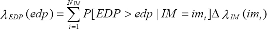
PEER’s framework for performance-based evaluation is encapsulated in a “framing equation” (Cornell and Krawinkler, 2000; Deierlein et al., 2003), a triple integral that integrates over the expected values of IM, EDP, and DM to compute the annual rate of exceedance of the DV, λ (DV). The triple integral equation may be written as Equation D.1:
 |
(D.1) |
where P[a|b] describes the conditional probability of a given b, ΔλIM is the annual probability of occurrence of IM = imi, and NDM, NEDP, and NIM are the number of increments of DM, EDP, and IM, respectively. This triple integral is solved numerically for most practical problems. Accuracy increases with increasing number of increments.
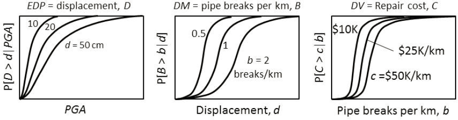
The conditional probabilities can be described by fragility functions that predict (i) the probability of exceeding the earthquake demand parameter, EDP, given the intensity measure, IM; (ii) the probability of exceeding the damage measure, DM, given the EDP; and (iii) the probability of exceeding the decision variable, DV, given the DM. Figure D.1 presents example fragility curves for the evaluation of the performance of a pipeline system subject to earthquake-induced ground displacement. In this case, PGA is used as the IM, lateral spreading displacement as the EDP, number of pipeline breaks per km as the DM, and repair cost as the DV. By combining the results of probabilistic response, damage, and loss models with the results of a probabilistic seismic hazard analysis, this approach can provide a consistent and objective evaluation of response, damage, and loss.
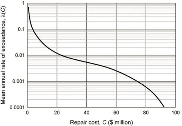
The quantity λ(DV) in Equation D.1 is computed for a range of DV values and presented in the form of a hazard curve for loss that describes how often, on average, different levels of loss can be expected to be exceeded (Figure D.2). λ (DV) is essentially equivalent to the annual probability of a particular loss level and the reciprocal of the return period. The hypothetical risk curve in Figure D.2 indicates a 1% annual probability (λ (DV) = 0.01) of $22 million in repair costs and a 0.1% annual probability (λ (DV) = 0.001) of $74 million in repair costs. This format allows an owner to treat expected annual losses as expenses in a cash flow analysis or to judge their cumulative effect over different exposure times to make decisions on loss mitigation (retrofit, insurance, abandonment, etc.) using cost-benefit analyses.
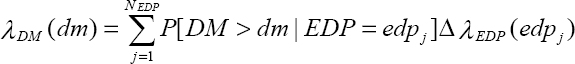
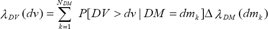
The PEER framework is modular—it can be formulated to produce response and damage hazard curves—which can be helpful for different implementations of performance-based evaluations. In modular form, Equation D.1 can be presented as:
 |
D.2 |
 |
D.3 |
 |
D.4 |
Equations D.2-D.4 are used in response-, damage-, and loss-level implementations.
THE HYBRID APPROACH
It is possible to treat some parts of the performance prediction process in a continuous manner and other parts in a discrete manner. For example, it is often difficult to characterize damage using continuous variables: the cracking of a concrete slab may be more readily characterized in qualitative damage categories (slight, moderate, severe) rather than continuous measures (e.g., cumulative length, crack width, and spacing), and the occurrence of a flow slide is binary—it either happens or it does not. In such cases, a damage probability matrix (Whitman et al., 1974) may be employed. To construct a damage probability matrix, the continuous range of EDP response levels is discretized into a finite number of bins; each EDP bin is associated with a damage state (e.g., negligible, slight, moderate, severe, and catastrophic); and values in each cell represent the probability of occurrence of the damage state given the EDP value. The matrix can be illustrated in tabular form as shown in Table D.1. The sum of each column is unity, providing that the EDP and DM intervals are mutually exclusive and collectively exhaustive.
TABLE D.1 Hypothetical Damage Probability Matrix for the Definition of DM|EDP Relationship
| Damage State, DM | Description | EDP interval | ||||
|---|---|---|---|---|---|---|
| edp1 | edp2 | edp3 | edp4 | edp5 | ||
| dm1 | Negligible | 0.90 | 0.50 | 0.30 | 0.15 | 0.05 |
| dm2 | Slight | 0.07 | 0.35 | 0.45 | 0.45 | 0.15 |
| dm3 | Moderate | 0.02 | 0.10 | 0.15 | 0.25 | 0.20 |
| dm4 | Severe | 0.01 | 0.04 | 0.07 | 0.10 | 0.30 |
| dm5 | Catastrophic | 0.00 | 0.01 | 0.03 | 0.05 | 0.30 |


