
7
Empirical and Semiempirical Methods for Evaluating Liquefaction Consequences
The consequences of liquefaction are described and illustrated in Chapters 1, 2, and 6 and can include vertical and lateral ground displacement; slumping and failure of embankments; loss of foundation support; increased lateral loads on and reduced lateral resistance of structures and their foundations; buoyancy uplift of buried structures; and modification of free-field ground motions. This chapter focuses on empirical and semiempirical methods for evaluating these consequences of liquefaction.
The complexity of the phenomena that follow liquefaction triggering has prompted the development of a variety of empirical and semiempirical procedures used by practicing engineers. These include screening procedures that employ damage indices to determine if the consequences of liquefaction are of engineering concern; procedures to evaluate the potential for lateral spreading, flow sliding, and slope instability; and procedures to evaluate the performance of deep and shallow foundations, earth retaining structures, subsurface utilities, and buried structures. While most of these procedures are logically formulated, and some are supported by laboratory and model testing, there is little field verification of these techniques (with the exception of some screening procedures). The lack of field verification may be attributed to the paucity of appropriately documented case histories of liquefaction consequences.
SCREENING PROCEDURES
Several procedures have been developed to screen sites for the potential for damage associated with liquefaction. Three types of screening procedures are used in practice: (1) a procedure that
establishes a threshold ground motion below which liquefaction damage is expected to be inconsequential; (2) a procedure to screen sites for damage potential based on the appearance of surface manifestations of liquefaction; and (3) procedures that use results from liquefaction triggering evaluations to compute a numerical index for the severity (extent) of triggering, which is presumed to correlate with liquefaction damage potential.
Threshold Ground Motions
The use of screening criteria to eliminate the need for a specific class of engineering analyses (i.e., exclusionary criteria) is common among federal, state, and local public works agencies. Federal Highway Administration (FHWA) guidance documents (see, e.g., FHWA, 2006) and American Association of State Highway and Transportation Officials (AASHTO) specifications also use earthquake magnitude and ground motion threshold criteria to determine if a liquefaction consequence assessment is needed at a bridge site. AASHTO (2014) specifications state that a liquefaction consequence assessment is not required for bridges designed to a life safety standard if the 5% damped design spectral acceleration at one second corrected for local site conditions, SD1, is less than 0.15 g, or 0.3 g if the liquefiable soil is low-plasticity silt. In addition, the AASHTO guide specifications do not require a liquefaction consequence assessment if groundwater is not within 50 feet of the ground surface and either the normalized standard penetration test (SPT) blow count, (N1)60, is greater than 30 blows/30 cm; the normalized cone penetration test (CPT) tip resistance, qc1N, is greater than 180 atmospheres; or the normalized shear wave velocity (VS1) is greater than approximately 213 m/s (700 ft/s). FHWA (2006) screens out the need for a liquefaction consequences assessment if SD1 is less than 0.25 and the site corrected spectral acceleration at a period of 0.2 seconds, SDS, is less than 0.35 g, or the earthquake magnitude is less than 6, or the earthquake magnitude is between 6 and 6.4 and either the normalized SPT blow count, (N1)60, is greater than 20 or (N1)60 is between 15 and 20 and SDS is less than 0.35 g. Despite the rather detailed specifics of these criteria, the study committee is not aware of any documentation of the development of these screening criteria, nor of any evaluation of their efficacy (e.g., comparison to case history data). Furthermore, these criteria are specific to bridges designed in accordance with AASHTO standards, including a life safety performance criterion, and should not be applied to structures other than bridges without some demonstration of their effectiveness.
Screening for Surface Manifestations
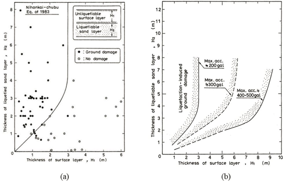
The influence of a non-liquefiable capping layer (of a thickness H1) on suppressing the surficial manifestation of liquefaction in an underlying liquefiable layer (of a thickness H2) was quantified by Ishihara (1985) based on field performance data. Ishihara related the minimum value of H2 necessary for liquefaction to manifest at the ground surface to H1 (i.e., to the non-liquefiable surface capping layer thickness). Figure 7.1 provides the H1-H2 boundary curves developed by Ishihara (1985) using a combination of field performance data from the 1976 Tangshan, China, earthquake, the May 26, 1983 M 7.3 Nihonkai-Chubu (Sea of Japan) earthquake, and professional judgment. The point at which one of those boundary curves becomes vertical represents a capping layer thickness beyond which no surface manifestation of liquefaction is expected to be observed regardless of the thickness of the underlying liquefiable layer. Later studies (Youd and Garris,
1995) supported the limiting thicknesses of capping layers shown in Figure 7.1 for surface manifestations other than lateral spreading and the transient ground movements referred to by Youd (1984) as ground oscillations. Experience in the 2011 Christchurch, New Zealand, earthquake indicates that while Figure 7.1 may be applicable to two-layer systems composed of a non-liquefiable capping layer overlying a liquefiable layer, it is difficult to apply this concept to stratified profiles with multiple liquefiable layers interbedded with non-liquefiable layers (van Ballegooy, 2012, 2014b). In addition, this method may not identify cases where settlement of a liquefiable layer does not result in surface manifestations such as differential settlement or cracking of the surficial soil layer. If settlement due to liquefaction beneath a non-liquefiable capping layer is of engineering concern, the engineer may wish to evaluate the potential for such settlement using methods discussed subsequently and to consider the engineering implications of the calculated settlement.
The concept described in Figure 7.1, however, is being used in New Zealand as guidance for mitigating liquefaction impacts to structures on shallow foundations by creating a uniformly non-liquefiable crust beneath the structure (van Ballegooy et al., 2015). While this concept has proven applicable to cases with a uniform non-liquefiable crust, the case history data used to support this concept are still limited, particularly with respect to earthquake magnitude and intensity; consequently, continued review of the applicability of Figure 7.1 using data collected in future earthquakes is warranted.
Liquefaction Severity Indices
Liquefaction severity (damage potential) indices are intended to provide a measure of the severity of surface manifestations based upon the cumulative liquefaction response of the profile. Various severity or damage potential indices have been proposed in the literature, among them: the Liquefaction Potential Index (LPI; Iwasaki et al., 1978); the Ishihara-inspired Liquefaction Potential Index (LPIISH; Maurer et al., 2015c); the one-dimensional volumetric reconsolidation settlement (S1VD); and the liquefaction severity number (LSN; van Ballegooy et al., 2012). These terms are defined and discussed in the following sections.
Liquefaction Potential Index (LPI)
The LPI, proposed by Iwasaki and colleagues (1978), provides a depth-weighted index of the potential for triggering of liquefaction at a site. As shown in Equation 7.1, LPI is computed as
| (7.1) |
The resulting index is therefore dependent on the thickness of liquefiable layers in the uppermost 20 meters, the proximity of these layers to the ground surface, and the amount by which the FS against liquefaction is less than 1.0. As opposed to the Ishihara (1985) procedure described above for determining the influence of a non-liquefiable crust over a single liquefiable layer, the LPI applies to a profile with multiple liquefiable layers. LPI can range from 0 (no layers with an FS less than 1 in the uppermost 20 meters of soils) to a maximum of 100 (the FS against liquefaction is zero for all layers in the uppermost 20 meters). Analysis of data from 45 sites that liquefied during the 1964 Niigata, Japan, earthquake showed that severe liquefaction occurred at sites where LPI > 15, and little liquefaction occurred where LPI < 5 (Iwasaki et al., 1978). Liquefaction hazard maps have been developed using the LPI framework for seismic regions in many regions of the world (see, e.g., Sonmez, 2003; Papathanassiou et al., 2005; Baise et al., 2006; Holzer et al., 2006a,b; Lenz and Baise, 2007; Cramer et al., 2008; Hayati and Andrus, 2008; Yalcin et al., 2008; Chung and Rogers, 2011; Dixit et al., 2012).
In more recent work by Maurer and colleagues (2015c), a power-law depth weighting function (i.e., 1/z, where z is depth) has been employed instead of the linear function used in the original LPI framework. Maurer and colleagues (2015c) also modified the LPI framework to account for the limiting thickness of the non-liquefiable capping layer central to the H1-H2 chart developed by Ishihara (see Figure 7.1b). The revised severity index that incorporated these modifications, named by Maurer and colleagues (2015c) the “Ishihara Inspired Liquefaction Potential Index,” or LPIISH, was found to reduce the number of false-positive predictions (i.e., cases where manifestations were predicted but not observed) in 60 case histories from six earthquakes in the Taiwan, Turkey, New Zealand, and the United States. Specifically, of the 60 case histories analyzed, 31% of no-manifestation cases had LPI < 5, while 100% of no-manifestation cases had LPIISH < 5. The LPI
and LPIISH performed equally well, however, in predicting true positives (i.e., cases where manifestations were observed as predicted), with 94% of such cases correctly identified with either index.
LPIISH is computed as
| (7.2) |
where
 |
and
 |
where H1 is defined the same as H1 in Figure 7.1, and z is the depth to the layer of interest in meters below the ground surface. Although LPIISH shows improved predictive capabilities over LPI, it nevertheless can still yield incorrect predictions of liquefaction consequences. As a result, there is still a need for further development of liquefaction damage indices if they are to be considered reliable.
One-Dimensional Volumetric Reconsolidation Settlement (S1VD) and the Liquefaction Severity Number (LSN)
Similar to LPIISH, LSN uses a power law depth weighting factor (i.e., 1/z) to determine the cumulative liquefaction response of a profile. It also includes contributions from all layers that have an FS < 2 (as opposed to the use of only layers with FS < 1 when calculating the LPI). LSN is computed as Equation 7.3, below:
| Equation (7.3) |
where εv is the calculated post-earthquake volumetric strain at depth z (in meters) expressed in decimal form. To compute volumetric strain, van Ballegooy and colleagues (2012) used the method proposed by Ishihara and Yoshimine (1992), as implemented by Zhang and colleagues (2002) with CPT data. In the method by Ishihara and Yoshimine (1992), discussed later in this chapter, the post-liquefaction volumetric strains are calculated as a function of the FS for liquefaction triggering.
Because the volumetric strains from the Zhang and colleagues (2002) relationship are self-limiting, LSN reaches a limiting maximum value as the FS decreases. This limiting value is a function of relative density of the soil, resulting in a maximum LSN for a given soil profile regardless of the ground motion intensity (e.g., peak ground acceleration [PGA]).
Similar to LPI, LSN correlated fairly well to the severity of surficial surface manifestations observed during the 2010-2011 Canterbury, New Zealand, earthquake sequence in areas where
liquefaction did not manifest in the form of lateral spreading and for profiles that did not have a clay capping layer or multiple non-liquefiable layers interbedded with the liquefiable layers (van Ballegooy et al., 2012, 2014a; Tonkin and Taylor, 2013; Maurer et al., 2014b, 2015a). The cumulative volumetric strain of the liquefiable layers in the soil profile, S1VD, was not as accurate as either LPI or LSN. Nevertheless, a comparison of the accuracy of LSN versus the accuracy of LPIISH was inconclusive (van Ballegooy et al., 2015).
Using Liquefaction Severity Indices
Liquefaction severity indices are useful in engineering practice for prioritizing sites for more detailed investigation and for regional hazard mapping, but they are not a substitute for more detailed analysis, and they do have limitations. Use of any of the methods described above assumes that the severity of surficial manifestations of liquefaction serves as a proxy for liquefaction damage potential. While this is likely a valid assumption for shallow foundation systems and surficial or near-surface infrastructure, it may not be valid for deep foundation systems. Furthermore, it has been found that damage indices based on the cumulative liquefaction response or volumetric strain potential of a soil profile are poor predictors of lateral spreading or flow sliding due to thin but continuous seams of liquefiable soil.
Even for non-lateral spreading manifestations, the severity thresholds reported in the literature for any of the aforementioned severity indices need to be used with caution. For example, several studies have shown that the correlation between computed LPI values and the observed severity of surface manifestation can depend on the procedure used to compute the FS against liquefaction and the fines content of the liquefied soil (Lee et al., 2003; Toprak and Holzer, 2003; Holzer et al., 2005; Juang et al., 2008; Papathanassiou, 2008; Maurer et al., 2014b, 2015a,b). In addition, because the LSN framework and threshold severity values were developed based on damage in a single geologic environment (i.e., Christchurch, New Zealand), their application elsewhere needs to be validated by comparison to field performance data from different environments.
Going forward, engineers need to keep in mind that these methods could be useful for preliminary assessments, but they are not suitable for detailed assessment of liquefaction consequences. Developers of severity index frameworks need to state explicitly the limitations of their methods and the significant sources of uncertainty associated with them. Continued calibration and validation of these methods against case history data—leading to improved analyses and ultimately to quantification of the uncertainty associated with them—is warranted.
FLOW SLIDING
Empirical and semiempirical procedures for analyzing flow slide potential rely typically on static limit equilibrium analyses (i.e., limit equilibrium analyses in which no seismic coefficient is employed) using the post-liquefaction shear strength of the soil in the liquefied zones and shear strengths appropriate for post-earthquake conditions elsewhere in the ground. If using those shear strengths results in an FS less than 1.0 it is usually assumed that flow sliding will occur if liquefaction is triggered. The resulting deformations are usually described qualitatively as large. If flow sliding is predicted, remediation often is assumed to be required. In some cases (e.g., for slopes supporting or adjacent to critical facilities), to provide an appropriate margin of safety, an FS greater than 1.0 may be considered a necessary threshold value. In other cases, however,
designing for an extreme level of earthquake shaking is assumed to account for all of the uncertainty in the assessment of the potential for flow sliding; an FS of 1.0 is then considered appropriate. This is implicitly the case in FHWA and AASHTO Load and Resistance Factor Design (LRFD) recommendations that call for a resistance factor of 1.0 for geotechnical design for the seismic design ultimate limit state (see, e.g., Kavazanjian et al., 2011). The committee is not aware of any quantitative assessment of reliability that can distinguish between these two approaches. Development of a reliability assessment framework that allows comparison of different simplified approaches to evaluating flow slide potential, and research on the parameter values required to implement such an assessment, are warranted and would provide a consistent means to incorporate uncertainties into flow sliding analyses.
No documented cases exist of flow failures that resulted from liquefaction of soils with an equivalent clean-sand normalized SPT blow count, (N1)60-cs, greater than about 15 blows/30 cm, or with a CPT tip resistance, qc1-cs, greater than about 85 atm. This raises the question of whether this absence of flow slide case histories implies that the post-liquefaction strength of soil increases sharply beyond these (N1)60-cs and qc1-cs threshold values (see Chapter 6) or if some other mitigating factor is involved. While it may be possible that liquefaction flow failures in such soils simply have not been documented, the frequency of observations of liquefaction triggering does not decrease significantly until (N1)60-cs reaches approximately 20 blows/30 cm and documented incidents of liquefaction triggering and liquefaction-induced lateral soil displacements include cases for (N1)60-cs up to about 26 blows/30 cm. The absence of case histories of flow failure for (N1)60cs values greater than 15 blows/30 cm and qc1-cs greater than about 85 atm, combined with the existence of case histories of triggering and lateral displacement for (N1)60-cs up to about 26 blows/30 cm, is strong circumstantial evidence that liquefaction-induced flow failure is unlikely when (N1)60-cs exceeds 15 blows/30 cm or qc1-cs is greater than about 85 atm.1 Nonetheless, in the absence of any alternative, when the post-liquefaction strength must be assessed for soils with (N1)60cs values greater than 15 blows/30 cm and qc1-cs greater than about 85 atm, the available correlations may be extrapolated beyond this point. There are no circumstances, however, when it is appropriate to use an extrapolated strength that is greater than the drained strength of the soil. Idriss and Boulanger (2008; see Figure 6.3) indicate with dashed lines the values extrapolated beyond (N1)60-cs equal to between 10 and 15 blows/30 cm. The curve for the case where void ratio redistribution effects are not expected to be significant becomes asymptotic when (N1)60-cs is equal to about 17 blows/30 cm. The curve for the case where void ratio effects are considered to be significant extends out to values of (N1)60-cs equal to 30 blows/30 cm, even though there are no case histories for (N1)60-cs greater than 15 blows/30 cm on the plot. Additional study on flow slide potential of soil characterized by penetration resistance values corresponding to (N1)60-cs of greater than 15 blows/30 cm and qc1-cs values greater than 85 atm would allow greater confidence in the use of extrapolated strength values and provide needed insight into the relationship between triggering and flow of denser liquefiable soils, even though the uncertainty in the residual strength of soils with high SPT resistance is high.
___________________
1 Most of the flow failure case histories are for slope gradients less than 10% and depths less than 10 meters. Caution is warranted when applying this finding to steep slopes with large initial static shear stresses and for critical structures such as large earth dams.
LATERAL SPREADING
If a site is susceptible to liquefaction triggering and assessment indicates that flow sliding is not anticipated, the potential for lateral spreading must still be evaluated. The lateral spreading case history databases include slope gradients as flat as 0.5%, so it is difficult to eliminate the potential for lateral spreading based on slope gradient alone. Four methods to estimate lateral spreading displacements are commonly used in practice (Idriss and Boulanger, 2008): (1) case-history-based empirical correlations with field soil and site parameters; (2) integration of permanent shear strains in the liquefied soil; (3) sliding block displacement analyses using limit equilibrium analysis with residual shear strength in the liquefied zones; and (4) computational-mechanics-based methods that employ two- or three-dimensional numerical simulations and constitutive models for liquefying soil. The first three methods are discussed in this section. Computational-mechanics-based approaches are described in Chapter 8. Probabilistic methods to evaluate lateral displacement are also introduced in this section and discussed in more detail in Chapter 9.
Case-History-Based Empirical Correlations
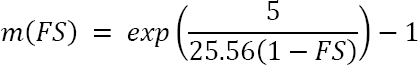
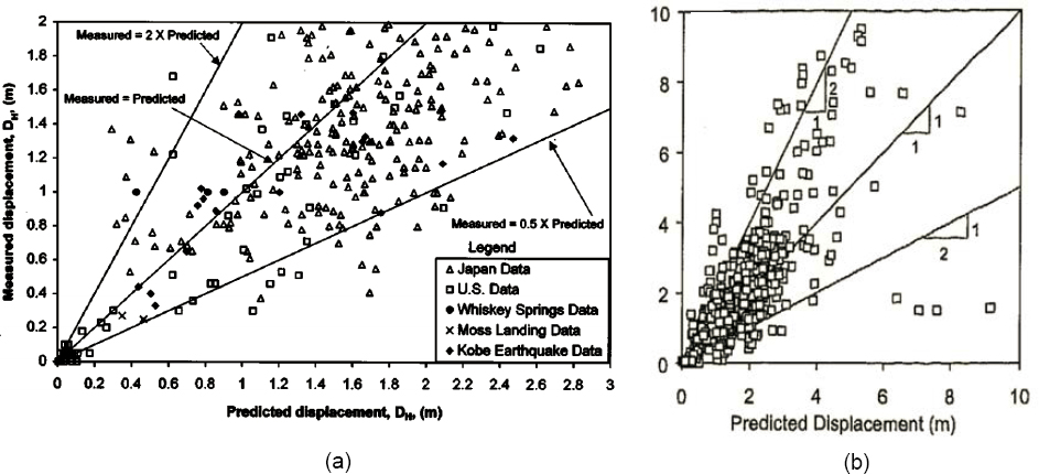
Empirical correlations by Rauch and Martin (2000), Bardet and colleagues (2002), and Youd and colleagues (2002) are among the methods available for assessing the amount of lateral spreading. Table 7.1 presents the key parameters used by these investigators. There are many common parameters among the different methods, although the precise definitions of those parameters and the collective set of parameters used by investigators vary. For instance, Bardet and colleagues (2002) and Youd and colleagues (2002) used a similar set of parameters in their respective lateral spreading models, chosen based on earlier work by Bartlett and Youd (1995). Bardet and colleagues (2002) omitted the grain size parameters employed by Youd and colleagues (2002), however, due to the difficulty in evaluating them from case history data. Rauch and Martin (2000) developed a hierarchy of three models of increasing complexity. Their regional model employed just four parameters: earthquake magnitude, distance from the site to the fault, PGA, and the duration of strong ground motion. Their site model also included general characteristics of the site (e.g., ground slope, height of the free face) in the regression equation, while their geotechnical (Geo) model also included the depth to the top of the liquefied zone and the depth to the liquefied zone with the lowest FS.
Figure 7.2 compares the observed and predicted displacements from the correlations by Bardet and colleagues (2002) and Youd and colleagues (2002). Figure 7.3 provides observed and predicted displacements from Rauch and Martin (2000). Figures 7.2 and 7.3 show that predictions made using these models may be as much as two times greater and smaller than half the measured displacement. In some of the models, the smaller the calculated displacement, the greater is the discrepancy between observed and predicted displacements. These models provide insight regarding the factors that influence lateral spreading potential and may be useful for gross screening assessments of lateral spreading potential (e.g., liquefaction hazard mapping, preliminary site assessments). Given the large uncertainty associated with the models, they are not suitable for detailed engineering analysis. Nevertheless, quantifying the uncertainty associated with these models to facilitate their use (e.g., to quantify the confidence limits on anticipated lateral spreading displacements) would benefit the technical community.
TABLE 7.1 Key Parameters Accounted for in Empirical Correlations for Lateral Spreading (indicated by check)
| Parameter | Youd et al. (2002) | Bardet et al. (2002) | Rauch and Martin (2000) |
|---|---|---|---|
| Moment magnitude | ✓ | ✓ | Regional,a Site,b Geoc |
| Distance to fault | ✓ | ✓ | Regional, Site, Geo |
| Depth to liquefiable layer | ✓ | Geo | |
| Ground slope | ✓ | ✓ | Site, Geo |
| Height of free face | ✓ | ✓ | Site, Geo |
| Distance from free face | ✓ | ✓ | Site, Geo |
| Free field PGA | Regional, Site, Geo | ||
| Strong motion duration | Regional, Site, Geo | ||
| Thickness of saturated granular soil layers with (N1)60 ≤ 15 | ✓ | ✓ | |
| Grain size | ✓ | ||
| Fines content | ✓ |
a Denotes a regional model that includes earthquake magnitude, distance from the site to the fault, peak ground acceleration, and the duration of strong ground motion.
b Denotes a site model that included the parameters above and general characteristics of the site (e.g., ground slope, height of the free face) in the regression equation.
c Denotes a geotechnical model that included the parameters above and the depth to the top of the liquefied zone, and depth to the liquefied zone with the lowest factor of safety.
Integration of Permanent Shear Strains
The permanent shear strain approach integrates the earthquake-induced permanent shear strain potential over depth to calculate a lateral spreading displacement at the ground surface. Zhang and colleagues (2004) refer to this integrated lateral displacement as the lateral displacement index (LDI). The LDI is calculated as Equation 7.4:
| (7.4) |
where zmax is the maximum depth at which liquefaction is expected, and γmax is the maximum possible permanent shear strain (evaluated at each depth, z). The maximum possible permanent shear strain at each depth, γmax(z), is related to the potential for liquefaction and the relative density of the soil. The relationships developed by Ishihara and Yoshimine (1992) are commonly used to estimate γmax. These relationships, presenting γmax as a function of the FS against liquefaction and the relative density of the soil, were developed from laboratory testing data of clean-sand specimens reconstituted at different relative densities. Larger values of γmax occur for smaller FSs and lower relative densities, but there is scatter in the data. The effect of fines content on strain potential is typically captured in practice through the same fines adjustments used for liquefaction triggering. The committee is not aware, however, of any demonstration that this approach is valid.
Zhang and colleagues (2004) combined the relationships from Ishihara and Yoshimine (1992) with the limiting shear strain values of Seed (1979) to calculate the LDI. Cetin and colleagues (2009a) developed an alternative model to estimate γmax using an expanded dataset of laboratory test results that predicts γmax as a function of blow count and the cyclic stress ratio (CSR).
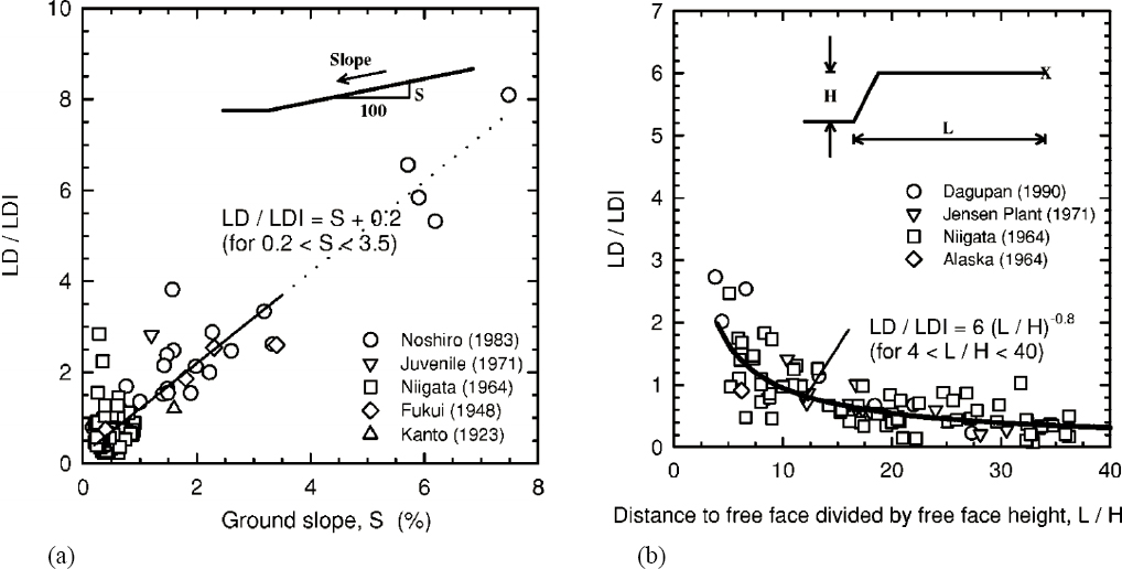
Comparison of computed LDI values with measured displacements at lateral spread sites (see, e.g., Shamoto et al., 1998; Tokimatsu and Asaka, 1998; Zhang et al., 2004) have shown that the LDI displacements have to be modified to account for site geometry factors such as the slope or
the distance to, and height of, a free face. For example, Zhang and colleagues (2004) evaluated the ratio of the observed lateral displacement (LD) to the LDI and found that this ratio increased with increasing ground slope (see Figure 7.4a) and decreased with increasing L/H, where L is the distance from the free face and H is the height of the free face (see Figure 7.4b). Even with corrections for ground slope and L/H, this approach does not appear to be more precise than are models derived from field case histories (i.e., accuracy generally within a factor of 2).
Faris and colleagues (2006) used an approach similar to the LDI to develop an equation for the maximum horizontal displacement of a laterally spreading site as a function of the equivalent clean-sand blow count, (N1)60-cs, the CSR, the slope gradient, α, and moment magnitude, M. These investigators first calculate a shear strain potential index (SPI) for each liquefiable layer as a function of (N1)60-cs and CSR. The SPI represents the maximum shear strain anticipated in the liquefiable layer and is based upon curves developed by Wu (2002) from laboratory test data predominantly for clean sands. Similar to the calculation of the LDI, the SPI is multiplied by the layer thickness and then summed over the site profile to obtain an estimate of Hmax. Based on mean values from a Bayesian analysis of case history data, Faris and colleagues (2006) proposed the following deterministic equation for Hmax:
| HMax = exp(1.0443 ln(DPImax) + 0.0046 ln(α) + 0.0029 M) | (7.5) |
where Hmax is in meters and α is shown as a percent.
Because this equation does not consider the possibility of a free face at the site, its use appears to be limited to sites where there is no free face. These investigators also use a fines content correction factor to adjust the blow count: that is, to evaluate (N1)60-cs, which is unique to their method. The equation does illustrate the influence of magnitude and slope gradient on lateral spreading, however, and shows that lateral spreading is possible even when there is no slope gradient: namely, in level ground (α = 0). Based on comparisons to the maximum displacement reported at lateral spreading sites, displacements predicted using Equation 7.5 appear to have levels of accuracy similar to other shear strain potential methods.
Given that permanent shear strain methods have accuracy of the same order of magnitude as the empirical equations described previously, they are subject to similar limitations: that is, they may be suitable for screening and preliminary analyses but are subject to considerable uncertainty when used for detailed engineering assessments. Furthermore, these models cannot capture the lateral displacement associated with a thin but continuous seam of liquefiable soil. The limited thickness of a thin seam of liquefiable soil would result in calculation of very small lateral displacements for even large permanent shear strain values, contrary to observations of lateral spreading due to thin liquefiable seams in the field. An improved level of accuracy and more information on the limitations and reliability of these models are needed to facilitate the use of these methods for detailed engineering analysis. While computational methods (discussed in the next section of this report) are not necessarily subject to any less uncertainty than these empirical methods, they do allow for greater detail and precision (though not necessarily greater accuracy) in engineering estimates of performance and should be considered for important projects as a source of additional information on the performance of engineered structures at a site that may be subject to lateral spreading.
Sliding Block Analyses
In a sliding block analysis (see Box 7.1) for lateral spreading, the yield acceleration (ky) for the potential sliding mass typically is established using pseudo-static limit equilibrium analysis with the residual shear strength(s) (implying large, unidirectional strains) assigned to the liquefiable layer(s) and post-peak large displacement strength(s) to non-liquefiable soil layer(s). As noted in the earlier section on flow sliding, this type of analysis is appropriate only if the static FS in a limit equilibrium analysis that uses these shear strengths is greater than 1.0. The yield acceleration is then found as the seismic coefficient (i.e., the lateral force coefficient used in the limit equilibrium analysis) that results in a limit equilibrium FS equal to 1.0. Predictive relations for permanent displacement as a function of the yield acceleration and seismological parameters (e.g., magnitude, site to source distance, PGA, peak ground velocity) derived by regression against the results of numerous sliding block analyses are available in the literature (see, e.g., Bray and Travsarou, 2007; Jibson, 2007; Anderson et al., 2008; Saygili and Rathje, 2008; Bardet and Liu, 2009; Lee et al., 2010; Rathje and Antonakos, 2011; Urzúa and Christian, 2013; Lee and Green, 2015). In Newmark-type analyses, these predictive relations can be used with ky evaluated—as discussed above—to assess lateral spreading potential in liquefiable terrain. Alternatively, an actual Newmark analysis can be performed using one or more design shear stress time histories. When actual time histories are employed, the time history is often obtained as the shear stress time history at the depth of sliding from a site response analysis in which potential modification of the ground motion due to pore pressure development is not considered.
These analyses are sometimes assumed to yield conservative estimates of the seismic displacement if ky is based on the assumption that the shear strength drops to the post-liquefied or large displacement value immediately at the initiation of strong ground shaking (Kavazanjian et al., 2011). Detailed comparisons, however, have not been made between observed lateral spread displacements and those computed from sliding block analyses. Furthermore, the displacements computed by a sliding block analysis are strongly influenced by the characteristics of the acceleration-time history, and liquefaction is known to change the characteristics of the acceleration-time history. While the accuracy of these types of analyses is unknown, they are sometimes considered to be more appropriate for evaluating lateral spreading on discrete soil layers than are other simplified methods (Olson and Johnson, 2008; Kavazanjian et al., 2011), and the argument that they are conservative (because they assume that liquefaction occurs immediately at the start of the earthquake) is logical.
Considering the alternatives for calculating lateral displacements due to liquefaction of a thin seam (e.g., Youd and Bartlett-type analyses), Newmark-type sliding block analyses for evaluating lateral spreading potential are likely to continue to be used for the near future. Nevertheless, comparisons between the results of sliding block analyses and deformations observed in documented case histories of lateral spreading, and perhaps from centrifuge experiments, are needed to assess the accuracy of these types of analyses in order to enhance the confidence associated with this type of analysis.
Probabilistic Design Acceleration
Many seismic hazard analyses today employ a probabilistically based horizontal PGA for design. One challenge using a probabilistically based design acceleration is that there is no unique earthquake magnitude associated with it. Similar to the method described in the Chapter 4 discussion of consideration of probabilistic design acceleration when calculating FS using the simplified method (Idriss, 1985; Finn, 2007), the levels of lateral spreading associated with the probabilistically based design acceleration can be evaluated using the deaggregated magnitude-distance information by calculating a lateral displacement for each magnitude-distance pair, multiplying that lateral displacement by the contribution of that magnitude-distance pair to the design acceleration, and summing up those displacements. It should be noted, however, that this is not a complete probabilistic representation of the lateral displacement because it ignores contributions to the displacement from events with other recurrence rates. To truly evaluate lateral displacement in a probabilistic manner, displacements must be integrated over the entire hazard curve using the performance-based design methodology described in Chapter 9.
LIQUEFACTION-INDUCED SETTLEMENT
Liquefaction-induced settlement can be attributed to a variety of mechanisms, including re-sedimentation or reconsolidation (volumetric strain) of the liquefied soil; ground loss due to venting of liquefied soil (i.e., sand boils or ejecta); settlement associated with lateral spreading under zero volume change; and settlement due to soil-structure interaction ratcheting and bearing capacity failure. Settlement associated with reconsolidation can be estimated quantitatively, but no simple or simplified quantitative models are available to estimate the settlement associated with ground loss due to venting of liquefied soil or to re-sedimentation of liquefied soil: namely,
settlement of liquefied soil where void ratio redistribution is significant beneath a capping low permeability layer, as defined by Idriss and Boulanger (2008). The average settlement (i.e., vertical displacement) associated with lateral spreading movements can be evaluated using the assumption of zero volume change of the sliding mass and the estimated lateral displacement. More detailed evaluation of the vertical settlement that accompanies lateral spreading likely requires using the computational-mechanics-based methods discussed in Chapter 8. Settlement due to soil-structure interaction that results from racheting has been shown by Dashti and Bray (2013) to be significant, but a method for predicting such settlements is not currently available. Similarly, procedures to assess bearing capacity failure, discussed later in this chapter, do not allow for assessment of associated settlement (although it is likely unnecessary to do so because a predicted bearing failure will generally require remediation).
Empirical analyses of settlement due to post-liquefaction reconsolidation typically assume free-field one-dimensional conditions. Under those conditions, the irrecoverable volumetric strain associated with pore pressure dissipation is equal to the vertical strain. This vertical strain can be integrated over depth to calculate the settlement due to reconsolidation. This calculation is the same as that described in the earlier discussion on the use of S1VD as an index for damage potential.
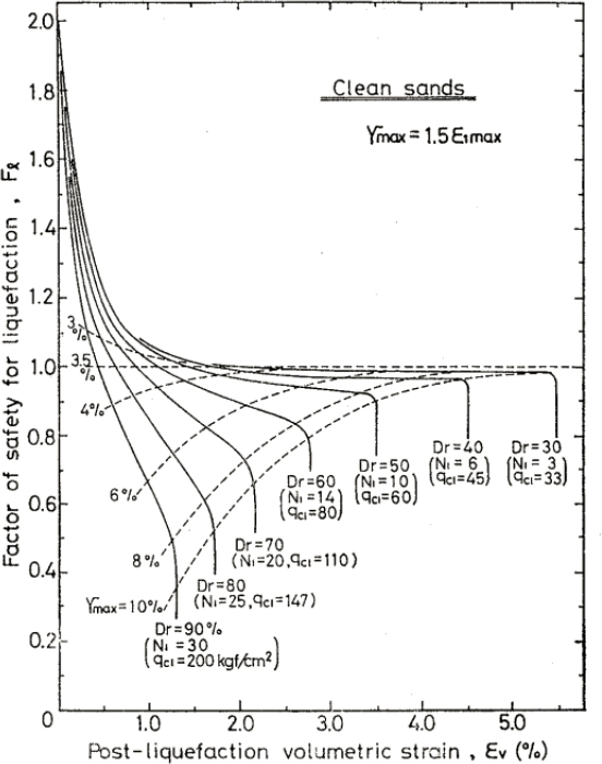
Various studies have shown that the post-liquefaction volumetric strain is influenced predominantly by the maximum shear strain and the relative density of the soil (see, e.g., Tatsuoka et al., 1984; Tokimatsu and Seed, 1987: Ishihara and Yoshimine, 1992). Tokimatsu and Seed (1987) developed a relationship between volumetric strain, SPT blow count, and CSR by combining data relating shear strain to volumetric strain with previously developed relationships between shear strain, SPT blow count, and CSR. Ishihara and Yoshimine (1992) related the volumetric strain to the FS against liquefaction and relative density (see Figure 7.5). Zhang and colleagues (2002) replaced the relative density term in Figure 7.5 with CPT tip resistance. These relationships can be represented by equations that predict volumetric strain as a function of the FS against liquefaction. Idriss and Boulanger (2008) also modified these relationships to be a function of SPT blow count or CPT tip resistance.
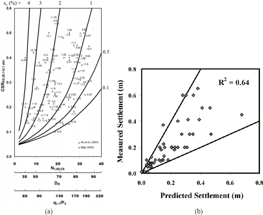
Cetin and colleagues (2009a) developed a model for post-liquefaction volumetric strain as a function of the clean-sand SPT blow count and the earthquake-induced CSR (see Figure 7.6a) similar to the model developed by Tokimatsu and Seed (1987). Cetin and colleagues (2009b) compared settlements computed by their model with measured settlements from 49 sites encompassing several earthquakes (see Figure 7.6b) and concluded that (1) the predictions were generally within a factor of 2 of the observed values, and (2) their model provided the best results among the several models they evaluated.
An important point is that the volumetric strain relationships discussed above are based primarily on laboratory data from testing clean sands. In practice, engineers typically use the equivalent clean-sand blow count or CPT tip resistance to calculate seismic settlement with these models, assuming implicitly that the effect of fines content is accounted for in the fines corrections for blow count or tip resistance. Studies of the effect of fines content on post-liquefaction consolidation settlement are limited. Laboratory simple shear testing on relatively undisturbed samples of sandy silt suggests that volumetric strains induced in liquefiable sandy silt were approximately the same as volumetric strains estimated from equivalent clean-sand blow counts (Reimer, 2007). These results are not necessarily contrary to findings from remedial ground densification projects wherein settlement (and therefore densification) is induced by liquefying the ground with techniques such as vibrating probes, weights dropped on the ground surface, and detonation of buried explosives. According to Elias and colleagues (2006), the effectiveness of these techniques in densifying the soil (i.e., inducing settlement) decreases with increasing fines content. Few comparisons between post-densification settlements of clean sandy soils and of silty soils in the field are available, however.
Observations show that in some cases damage from liquefaction-induced settlement may be closely associated with sand boils, which are symptomatic of subsurface ground loss (i.e., venting of liquefied soil). Ground settlement associated with sand ejecta accounted for nearly 90% of the land damage in residential neighborhoods resulting from the 2011 earthquake in Christchurch, New Zealand (van Ballegooy et al., 2014a). Differential subsidence associated with ground loss due to sand ejecta in this earthquake is documented to have exceeded the settlement expected due to free-field reconsolidation of the liquefied soil and to have been at least partly responsible for differential settlement that damaged commercial structures in the central business district in this earthquake (Bray et al., 2014). In addition to the structural distress associated with sand ejecta, some areas in Christchurch impacted by large amounts of ejecta subsided so that the land surface is now below high tide (Rogers et al., 2014). While there are no quantitative analyses for total and differential settlement due to ground loss following liquefaction, the liquefaction severity indices discussed previously appeared to correlate well with observations of excessive settlement in Christchurch and may provide at least an indication of how serious a problem liquefaction-induced settlement may be.
DEEP FOUNDATIONS
The potential consequences of liquefaction associated with deep foundations include loss of vertical bearing capacity, loss of lateral stiffness and capacity, lateral loading due to lateral soil displacements, and downdrag on piles due to post-liquefaction reconsolidation of soil. These consequences may be divided into inertial effects (i.e., those that impact the dynamic response of the pile foundation) and kinematic effects (i.e., those induced by soil displacement relative to the foundation). Inertial and kinematic effects on deep foundations are often considered separately
because the available simplified methods cannot account for them as coupled phenomena. This is justified because the peak inertial loads are likely to occur before the soil liquefies and begins to flow because the intensity of the ground motion subsequent to liquefaction will be reduced and, thus, the peak inertial load can be considered separately from the kinematic loads due to liquefaction-induced displacements (Kavazanjian et al., 2011). The primary inertial interaction effect prior to liquefaction-induced displacements is a reduction in lateral stiffness of the foundation, which can be considered in the inertial loading analysis (as described subsequently). The other effects cited above (loss of vertical and lateral capacity, lateral loading due to lateral soil displacements, and downdrag on piles due to post-liquefaction reconsolidation of soil) will occur only after triggering and, therefore, may be assumed to be independent of the dynamic response of the foundation system. Alternatively, an advanced computation model such as those discussed in Chapter 8 can be used to consider all inertial and kinematic loads together.
Vertical Capacity
The committee is not aware of formal procedures to account for the effect of liquefaction on the vertical capacity of a deep foundation element (e.g., a pile or drilled shaft, referred to generically herein as a pile). Seismic distress due to a reduction in vertical capacity induced by soil liquefaction has never been documented. In practice, the vertical capacity of a deep foundation is generally calculated as the sum of its side resistance and tip resistance. When considered in an engineering analysis, the loss of vertical capacity of a pile in liquefied soil can be accounted for by setting the side resistance of the pile in the liquefied zone to zero and by reducing the strength of end bearing soils expected to liquefy to their post-liquefaction strength. While there are few field or model test data to support this approach, in the absence of information to the contrary, this approach is a reasonable means of accounting for the influence of liquefaction upon vertical pile capacity based on the engineering mechanics of the problem. Nonetheless, it would be prudent to validate this assumption through centrifuge model testing and, should appropriate case history data become available, analysis of case histories.
There is a lack of consensus as to whether deep foundation elements in liquefiable soil are subject to downdrag, wherein settlement of a non-liquefiable crust due to reconsolidation of underlying liquefied soil pulls down on the sides of the pile. Logically, it is not necessary to consider downdrag loads imposed by reconsolidation if the liquefied soil is above the neutral plane of a driven pile. The pile has already been loaded by the soil above the neutral plane. If the soil above the neutral plane liquefies and subsequently reconsolidates and reloads the pile, and the soil below the neutral plane of the pile has not liquefied, then no significant settlement will occur. If the soil below the neutral plane liquefies, as may be the case, for instance, for a bored pile that has its neutral plane near its top, then settlement may occur due to the transfer of load down to the deeper soils.
Establishing whether or not downdrag should be considered, and validation of the approach generally used to consider it, is stymied by the lack of case history data on downdrag on piles in liquefiable ground. The Juan Pablo II bridge performance during the 2010 Maule, Chile, earthquake provides a rare case of seismic distress of a pier-supported structure due to reduction in the vertical capacity induced by soil liquefaction (Ledezma et al., 2012). More case histories of this effect are needed, however. Appropriate instrumentation and monitoring systems need to be installed to capture field evidence of downdrag in areas where seismic loading resulting in liquefaction is anticipated. Until appropriate data are available to evaluate whether downdrag is of concern, it is prudent to consider downdrag when evaluating deep foundation performance.
Lateral Stiffness
The reduced lateral stiffness of deep foundations in liquefied soil is accounted for in a simplified manner by reducing the lateral resistance of the liquefied soil in a p-y lateral load analysis. A p-y analysis treats the pile as a beam on an elastic foundation with a load-dependent or a displacement-dependent elastic response described by a curve relating the load, p, on a segment of the pile to the corresponding lateral, displacement, y (Reese et al., 1974). Essentially, each segment of the pile is supported by a spring, and the displacement-dependent spring stiffness is characterized by the p-y curve. This type of analysis is akin to an equivalent linear site response analysis in that iterations are performed until a displacement-compatible stiffness is arrived at using the nonlinear p-y curve. Alternatives to this type of simplified analysis are advanced
computational methods (see Chapter 8) wherein either the soil is modeled as a series of nonlinear springs attached to the foundation elements or a continuum soil model is used along with structural elements and interface elements.
The reduced lateral resistance of liquefied soil in a p-y analysis is usually accounted for in one of three ways: (1) by using a reduced undrained shear strength in the liquefied zone and developing the p-y relationship by applying rules to develop p-y curves for the undrained behavior of fine-grained soil (Abdoun, 1997; Wang and Reese, 1998); (2) by using a multiplicative factor (i.e., a p-multiplier) that is less than 1 to modify the p-values of the p-y curve for the non-liquefied soil (Liu and Dobry, 1995; Wilson, 1998; Ashford et al., 2011); or (3) by using a constant pressure against the piles in the liquefied zone. Based on an analogy with post-liquefactions stability assessments, it is often assumed that the residual shear strength can be used as the reduced shear strength of liquefied soil. But, based on centrifuge test results, Abdoun (1997) found that the lateral resistance of a single pile in liquefied loose sand could be represented by assigning an undrained shear strength of approximately 1 kPa to the liquefied soil, a value significantly less than what would be calculated using the post-liquefaction undrained strength. The centrifuge tests were reinterpreted, and it was recommended that a constant pressure of 10.3 kPa be applied to a pile in liquefied soil (Dobry et al., 2003). There was good agreement reported between calculated and observed values when this assumption was used to calculate pile bending moments with two field case histories given the assumption that non-liquefied soil above the liquefied zone applied passive pressure to the foundation system (e.g., pile and pile cap).
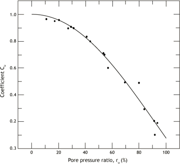
Data from centrifuge model tests on clean sand with a relative density of 40% from Liu and Dobry (1995) was employed to develop the plot in Figure 7.7 of p-multiplier (called Cu in Figure 7.7) versus excess pore pressure ratio (ru). Note that at an excess pore pressure ratio of 1.0, representative of liquefaction, the p-multiplier is approximately 0.1, so the lateral resistance of the liquefied soil is approximately 10% of its initial value. But, p-multipliers on the order of 0.25 have been reported for liquefied soil based on centrifuge model tests (Ashford et al., 2011). Furthermore, assigning a reduced p-y resistance in the liquefied soil may be inappropriate because of the generally gradual buildup of pore pressures during an earthquake, and because the reduction in p-y resistance does not exceed 0.5 until the pore pressure ratio equals 70% (as illustrated in Figure 7.7).
Centrifuge tests simulating lateral pile performance in liquefied denser sands (Wilson et al., 2000) and lateral load tests on piles in soil liquefied by blasting (Rollins et al., 2005) show stiffening due to shear strain dilation at large deflections as well as a different backbone curve (i.e., for the locus of the tips of the hysteresis loops from uniform cyclic loading) than conventionally assumed for p-y curves. Chang and Hutchinson (2013) have observed similar behavior in shake table tests. A hybrid p-y model to account for this effect has been developed by Franke and Rollins (2013).
There remain many uncertainties as to the nature of post-liquefaction p-y curves for laterally loaded pile analyses. The influence of factors such as the gradual development of earthquake-induced pore pressures, cyclic loading amplitudes, pile displacement induced pore pressure, pore pressure dissipation, and the p-y resistance behavior of low-plasticity silts are among the major uncertainties. Investigations of influence of these factors on the p-y behavior of liquefied soil using centrifuge model and large-scale field tests and by study of field behavior of laterally loaded piles in earthquakes captured through instrumented sites are needed to facilitate development and validation of models for laterally loaded piles in different types of liquefiable soil.
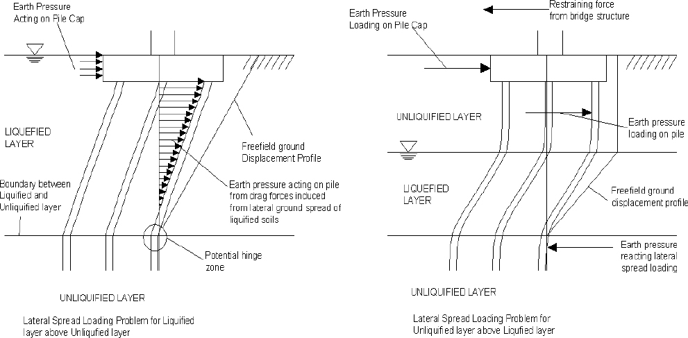
Loads Due to Lateral Spreading
Lateral spreading due to liquefaction can impart significant loads and displacements on deep foundations as well as on the structures supported by the displaced foundation elements. This type of loading is sometimes referred to as kinematic loading. In a structural analysis, kinematic loading can be accounted for in a simplified manner by displacing the foundations of the structure by an amount equal to the calculated free-field seismic displacements. This approach, however, ignores the interaction between the displaced foundation elements and the structure they support as the structure resists the foundation displacement. Properly accounting for such soil-structure interaction effects is not amenable to the use of simplified models; it requires use of computational models that include both structural and foundation elements (see Chapter 8).
As noted in the introduction to the section on deep foundations, in a simplified analysis, kinematic loading of deep foundations due to lateral displacement of the soil surrounding a pile subsequent to liquefaction is often decoupled from inertial loading from the superstructure (i.e., the two types of loading are considered independently) (POLA, 2010; POLB, 2012). Note that this decoupled assumption applies only after the soil has liquefied, and that inertial and kinematic interaction effects prior to the onset of liquefaction cannot be treated in a decoupled manner. Two kinematic loading situations often encountered in practice are depicted in Figure 7.8. In the first case, the zone of liquefaction extends to the ground surface and the liquefied soil tends to flow around the piles, applying relatively modest loads on the piles. In the second case, the zone of liquefaction lies below a non-liquefied crust that exerts relatively large loads on the piles. In both cases, the kinematic load imposed on the piles by laterally spreading soil can be evaluated using a p-y analysis in which the soil stiffness in the liquefied zone is reduced in the manner described
previously. The kinematic load is applied to the pile by displacing the supports for the p-y springs by an amount equal to the calculated free-field lateral displacement. This approach to the kinematic loading problem is described by Martin and colleagues (2002) and documented in an NCHRP Report (2002).
Ishihara and Cubrinovski (2004) used a reduced soil stiffness in the liquefied zone to analyze the response of a pile-supported liquefied petroleum tank subject to lateral spreading in the 1995 Hyogo-ken Nanbu (Kobe, Japan) earthquake. The situation analyzed by these investigators is the case on the right-hand side of Figure 7.8, that of a non-liquefied crust overlying the liquefied layer. In their analysis, Ishihara and Cubrinovski evaluated system performance for stiffness reduction factors of 100 and 1,000. Good agreement with observed behavior was reported for both reduction factors, leading the investigators to conclude that the stiffness of the soil in the liquefied zone had little impact on the predicted structure response.
Centrifuge tests to evaluate the p-y analysis approach to kinematic loading are described by Brandenburg and colleagues (2007). McGann and colleagues (2012) describe a detailed evaluation of this approach versus a three-dimensional finite element analysis. And McGann and Arduino (2014) document a case history study using both a finite element and a p-y approach. The use of the p-y approach for design is further described by Ashford and colleagues (2011).
Although this simplified approach to kinematic loading has been adopted in some seismic design standards (POLA, 2010; POLB, 2015), many uncertainties remain in this type of analysis, including, the validity of using the Newmark sliding block method to determine free-field displacements; the uncertainties related to residual strength of liquefied soils and related p-y curves; the uncertainties related to the thickness of the liquefied layer and the displacement distribution in the layer; the influence of potential partial pore pressure increases in adjacent soil layers; and the accuracy of the method in determining the distribution of pile bending moments.
Decoupling kinematic loading and inertial loading may not be appropriate for all situations, especially for large-magnitude events where earthquake shaking is of such duration that lateral spreading can induce kinematic loading on piles while strong shaking is still taking place. Some design standards require coupling the two loading conditions (POLB, 2012; ASCE, 2014). Clear guidelines on how to couple the kinematic and inertial loads are not provided in these design standards, but Ashford and colleagues (2011) do provide guidance on their coupling.
Ultimately, data from instrumented deep foundations subject to lateral loading are needed to validate these methods. It will take multiple earthquakes in extensively instrumented areas, however, to provide those data. In the interim, some uncertainty can be reduced through laboratory and field model testing supplemented by advanced numerical models (Chapter 8). Sensitivity studies, such as those performed by Ishihara and Cubrinovski (2004), are needed to assess system performance over the range of possible values for design parameters (e.g., the reduced pile resistance in liquefied soil).
SHALLOW FOUNDATIONS
In most cases where liquefiable soils are present beneath or adjacent to the footprint of a new structure, either the potential for liquefaction is mitigated or the deep foundations are used. Shallow foundations are, in general, avoided in such cases, but before liquefaction analysis was mandated by codes or was commonplace, structures underlain by liquefiable soil may have been constructed. Furthermore, since shallow foundations are relatively inexpensive compared to deep foundations, they may still be used when liquefaction-related deformations are expected to be small (City of Los Angeles, 2014). Bearing capacity may be estimated using post-liquefaction shear strength for the liquefied soil beneath the foundation. If a bearing failure is indicated, there usually is no need to assess the associated displacements because remediation is generally necessary.
The displacement of shallow foundations in liquefiable soil is often analyzed using the decoupled kinematic loading approach for deep foundations discussed above. Liquefaction-induced displacements, including lateral spreading and vertical settlement, are calculated and applied to foundation soil as displacements (i.e., as a kinematic load), distorting the structure without applying any inertial load. The forces and moments induced in the structure by this distortion are then computed in a structural analysis. In a simplified analysis, the calculated displacements are generally free-field displacements, ignoring any interaction between the ground and the structure (e.g., any restraining effect the structure may have on the induced displacements). Until recently, there were few data of any kind (e.g. model test data, field data) with which to validate this approach. Computational and physical (centrifuge) modeling by Dashti and Bray (2013), however, and case histories from the 2010-2011 Christchurch, New Zealand, earthquake sequence (Bray et al., 2014) have indicated that the decoupled approach can significantly underestimate liquefaction-induced displacements. These data need to be used in studies to develop appropriate simplified analyses for the performance of structures supported by shallow foundations on liquefiable soils.
RETAINING STRUCTURE DAMAGE
Soil liquefaction behind an earth retaining structure will increase the lateral earth pressure (i.e., the active thrust) on the structure. Liquefaction of soil in front of an earth retaining structure will reduce the lateral resistance (i.e., the passive resistance) of the structure. Liquefaction of soil beneath a retaining structure can result in loss of bearing capacity and lateral sliding resistance as well as vertical settlement. These effects in lateral earth pressure have led to bulging, tilting, and sliding of the retaining structures and damage to structures behind the retaining structures when not accounted for in design. Damage to earth retaining structures in the Port of Kobe in the 1995 Hyogo-ken Nanbu earthquake, described briefly in Chapter 1, is a notable example of this kind of damage.
Lateral earth pressures due to liquefied soil are generally accounted for using an equivalent fluid pressure concept. Both active thrust and passive resistance are calculated as equivalent fluid pressures based on the total unit weight of the liquefied soil (Ebeling and Morrison, 1993). This approach has been found to be consistent with observations of damage to earth retaining structures supporting liquefied soil in earthquakes (Iai, 1998), indicating the validity of this approach.
UTILITIES AND BURIED STRUCTURES
Damage to utilities (e.g., pipelines, sewer lines and storm drains, communications cables) due to liquefaction-related phenomena, including lateral spreading, settlement, buoyancy forces, and ground oscillation (or transient ground movements without permanent ground deformation), is common in large earthquakes in urban areas. Analyses of the impact of liquefaction on utilities include screening analyses of system wide performance and analyses of the performance of discrete components subject to liquefaction-induced ground deformations.
Screening procedures have been developed to evaluate the expected severity of damage to utilities from liquefaction-induced effects for use in loss estimation and for prioritization of more detailed system-wide assessments of damage potential. Loss estimation programs such as Hazus2 typically have such procedures built into them, and some public works agencies (e.g., the Los Angeles Department of Water and Power) have their own in-house screening procedures. The American Lifeline Alliance has developed procedures and equations to estimate the frequency of repairs needed to pipelines as a result of earthquakes and permanent ground deformation (ALA, 2001). These take into account such factors as pipeline material, joint type, corrosivity of soils, and the permanent ground deformation.
Such screening assessments are useful not only for loss estimation and prioritization of more detailed analyses for system upgrades but also for estimating system outage times and in planning for repair crew needs following a major earthquake. Every major earthquake provides an opportunity to refine such analyses. Often, however, they are not suitable for site-specific damage potential assessments.
Simplified analysis of the impact of liquefaction-induced ground deformations on pipelines and other linear utilities is typically accomplished using the decoupled kinematic loading approach discussed previously (i.e., by conducting a structural analysis in which calculated free-field ground deformations are imposed on the structure without any inertial load). As noted previously, this
___________________
ignores the impact of the structure on the ground displacement—a generally conservative assumption, as, due to its stiffness, the structure typically restrains the ground to some extent.
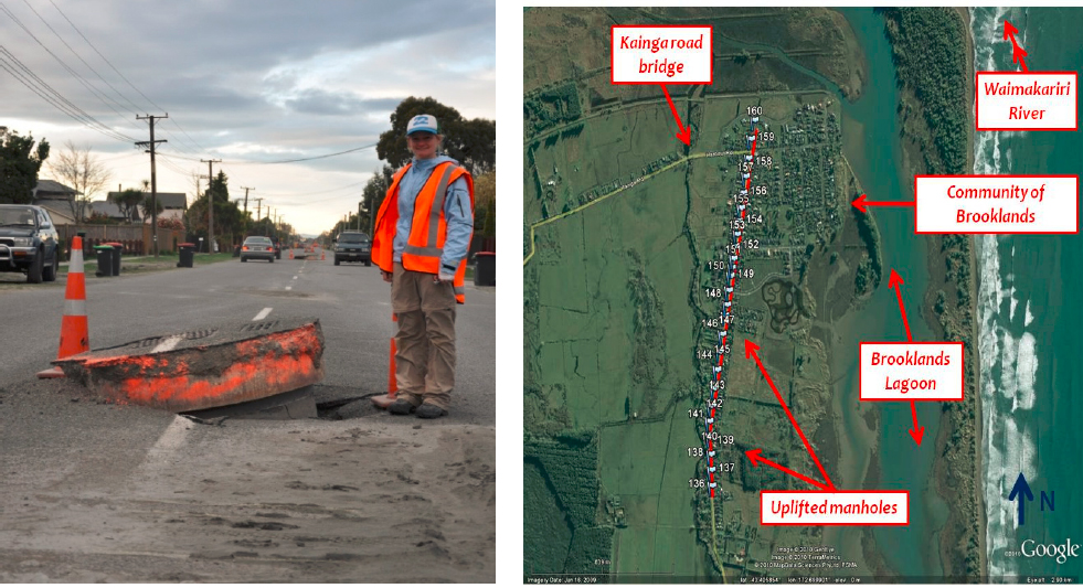
A common observation in liquefied soil in earthquakes is buoyant uplift of underground structures. Figure 7.9 shows a series of sewer manholes that buoyed up along a residential street during the 2010 Darfield, New Zealand, earthquake (GEER, 2010). Buoyant uplift can be accounted for by treating the liquefied soil as an equivalent fluid with a unit weight equal to the total unit weight of the soil and calculating the uplift force based upon the volume displaced by the underground structure (Tobita et al., 2012). This approach, however, is applicable only to isolated, unrestrained structures that are not laterally restrained either by structural considerations or by non-liquefied soil zones.
In the past decade, state-of-the-art research on the performance of pipelines—including sewer, potable water, and fuel—in liquefiable ground has been conducted (see, e.g., O’Rourke, 2010; O’Rourke et al., 2014). Models for both screening and detailed analyses of the performance of underground utilities in liquefiable soil were developed. Chou and colleagues (2011) have illustrated the use of centrifuge modeling and advanced computational analyses to predict the behavior of a sunken tube tunnel (the Bay Area Rapid Transit system tunnel) across San Francisco bay. Chou and colleagues (2011) illustrated that buoyant uplift alone may not be sufficient to predict the response of buried structures in liquefied soil if they are restrained laterally. In such cases, more sophisticated soil-structure interaction analyses such as those discussed in Chapter 8 are required to evaluate the performance of a buried structure in liquefied soil. There have also been some salient observations of pipeline performance during earthquakes in liquefied soil. A notable example is the observation that fusion-welded polyethylene pipe, almost without exception, did not rupture when subject to liquefaction and lateral spreading in the 2011 Christchurch, New Zealand, earthquake despite ground displacements of a meter or more (O’Rourke et al., 2014).
LIQUEFACTION-INDUCED MODIFICATION OF GROUND MOTIONS
The triggering of liquefaction and associated soil softening can significantly influence wave propagation through the liquefied zone and, thus, also influence the nature of ground surface motions. Until recently, few strong motion recordings were available at sites that liquefied, but such data now allow empirical evaluation of the effects of liquefaction on ground surface motions and validation of the ability of nonlinear, effective stress site response analyses to predict this effect.
Youd and Carter (2005) examined acceleration response spectra3 derived from ground motion records at five instrumented sites in liquefiable soil. They found a general reduction of short-period spectral accelerations (spectral period < 0.7 seconds) and amplified long-period spectral accelerations (spectral period > 0.7 to 1.0 sec) at those sites compared to sites without liquefaction. Hartvigsen (2007) investigated the effects of pore-pressure generation on ground surface motions by comparing results from nonlinear, one-dimensional effective stress analyses, and total stress analyses of hypothetical liquefaction sites, and found results in general agreement with those from Youd and Carter (2005). Evaluation of field data by Gingery and colleagues (2014) showed spectral acceleration amplification factors of about 1.8 to 3.1 in liquefiable soil profiles, findings generally consistent with those of Youd and Carter (2005) and Hartvigsen (2007). Gingery and colleagues (2014) also found modest amplification at spectral periods less than 0.05 seconds, which they suggest may be attributed to “acceleration spikes that occur in association with the dilational part of liquefaction phase transformation behavior”: that is, with short-period spikes in the ground motion acceleration due to stiffening of the liquefied soil as a result of its tendency to increase in volume when sheared. Anderson and colleagues (2011) make a similar observation with respect to the impact of dilation in their effective stress analysis of seismic site response (i.e., that it can amplify the short-period spectral content of ground motions).
The amplification factors proposed by Gingery and colleagues (2014) provide a means of assessing the potential impact of liquefaction on ground motions at a site in the long-period range. These factors are based on a small set of data, however; therefore, they may not reflect the full range of conditions encountered in practice. Effective stress site response analysis of the type conducted by Anderson and colleagues (2011) may be able to capture short-period amplification effects, though this type of analysis (i.e., an analysis that considers dilation during phase transformation) is not widely available. The limited field data and analytical studies on the effects of liquefaction on ground motion do not provide enough information for development of a simplified empirical or semiempirical approach to predicting with confidence the effect of liquefaction on site response, either before or after triggering. Similarly, nonlinear effective-stress site-response analyses have not been well validated in the post-triggering range and, therefore, need to be used with care. Additional ground motion recordings at borehole array sites that record shaking below the liquefaction layers and at the ground surface are needed to validate nonlinear effective-stress numerical models for site response.
__________________
___________________
3 An acceleration response spectrum is a plot of the maximum acceleration (referred to as the spectral acceleration) of a linear single degree of freedom system versus the natural period of the system (referred to as the spectral period). It provides the ground motion input to the most common type of structural analysis in earthquake engineering, modal superposition, and may be considered as a unique signature, or fingerprint, of the earthquake ground motion.


