2

Estimating Exposure and Effects of Sound on Wildlife

INTRODUCTION

The world is a cacophony of sounds—from natural sources such as wind-blown vegetation and ocean waves or calling insects, birds, fish, and whales—so all animals have evolved mechanisms to modify their vocalizations to compensate for noise and to focus as listeners on relevant sounds (Tyack and Janik, 2013). However, the increasing levels of anthropogenic noise create acoustic conditions unprecedented in the evolutionary record (Swaddle et al., 2015). Worldwide expansion of human activities and infrastructure is increasing the exposure of terrestrial and marine environments to anthropogenic sound (Hildebrand, 2009; Barber et al., 2010; Shannon et al., 2015). Recent estimates suggest that more than 88% of the contiguous United States experiences elevated sound levels due to anthropogenic activities (Mennitt et al., 2013) and that the propulsion noise from ships elevated ocean sound levels in the 25-50 Hz band by 8-10 decibels (dB) from the mid-1960s to the mid-1990s, which then remained constant or showed a slight decline in the next decade (Andrew et al., 2011).

Most of the human activities that produce noise are common to terrestrial and marine ecosystems. These include transportation, exploration for and extraction of oil and gas, construction, mining, and military operations. Sounds from these sources can influence terrestrial and marine animals in similar ways. Although this report focuses on the cumulative effects of anthropogenic stressors, including sound, on marine mammals, recent terrestrial studies have evaluated consequences of noise exposure in ways that have not been thoroughly investigated in marine mammals, such as declines in foraging efficiency (owls [Mason et al., 2016; Senzaki et al., 2016] and bats [Siemers and Schaub, 2011; Bunkley and Barber, 2015]), heightened vigilance (prairie dogs [Shannon et al., 2014, 2016] and songbirds [Quinn et al., 2006; Ware et al., 2015]), declines in reproductive success (Halfwerk et al., 2011), and altered predator–prey relationships (Francis et al., 2009). Insights from such terrestrial research help point to potential effects that deserve more attention in marine studies, and these studies can serve as guides for future efforts to determine whether noise affects marine mammals in similar ways.

Because research on land and at sea has largely progressed in isolation, we summarize the research status of each ecosystem separately below. Nevertheless, research in these disparate ecosystems provides a general framework for investigating how diverse noise stimuli present a multitude of challenges to wildlife.

When assessing the potential influence of a sound stimulus on an animal, determining whether the stimulus is within the organism’s sensory capabilities is critical. Most animals have developed sensory organs that allow them to detect either pressure waves or particle motion in the environment somewhere in the range of frequencies from below 10 Hz to above 180 kHz. They use this sensory input to communicate, orient, avoid predators, detect prey, and monitor their environment. If the stimulus falls outside of an animal’s sensory capabilities, i.e., higher or lower in frequency than its sensory organs can detect, the stimulus is likely not to have a direct effect (Francis and Barber, 2013), although indirect consequences of noise exposure are possible (e.g., Francis et al., 2009, 2012a).

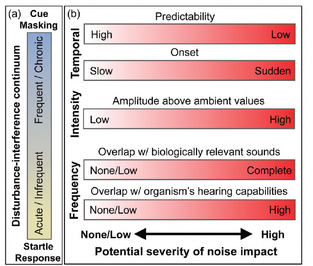
There is a diverse array of anthropogenic sound sources, which vary in time, frequency, and intensity. Variation along these axes is not only relevant to the detection capabilities of an organism’s sensory system, but is also relevant to how organisms perceive sound stimuli. Sounds that are sudden, unpredictable, and loud often generate startle responses that can be similar to those associated with predation risk (see Figure 2.1). Sounds with these characteristics need not be

associated with real threats to elicit strong responses. For example, the acoustic startle response in mammals is stimulated by sounds that increase to 80-90 dB above the threshold of hearing in 15 milliseconds (Fleshler, 1965). Götz and Janik (2011) demonstrated that the startle responses triggered by these stimuli are aversive enough to lead grey seals (Halichoerus grypus) to show fear conditioning with strong flight responses. Other sounds that animals interpret as originating from either predators or aggressive conspecifics may evoke disturbance responses similar to those that function to defend against risk of predation (Frid and Dill, 2002) or potential intraspecific confrontation. Beaked whales (Mesoplodon densirostris) respond to military sonar through antipredator behavior in a manner similar to, albeit less intense than, their responses to playback of predator calls (killer whales [Tyack et al., 2011]). Military sonar sounds in the 1-10 kHz band are well below the frequencies used in beaked whale vocalizations and those at which they hear best, but these sonar signals share a similar duration and frequency structure with the stereotyped calls of killer whales. The stronger response of killer whales (Orcinus orca) than that of sperm whales (Physeter macrocephalus) or long-finned pilot whales (Globicephala melas) to playbacks of sonar signals (Miller et al., 2012; Harris et al., 2015) suggests that killer whales also perceive the sonar as threatening.

Sounds that are frequent, continuous, or chronic may not be perceived as threatening but nonetheless can affect animals by interfering with their ability to detect acoustic signals or cues, such as calls from conspecifics or sounds made by predators or prey (see Figure 2.1). The more overlap there is in spectral bandwidth between anthropogenic sounds and those used by an organism, the more likely they are to interfere with detecting biologically important signals. Masking of relevant sounds has the potential to reduce an organism’s auditory perceptual range, or listening area (Payne and Webb, 1971; Clark et al., 2009; Barber et al., 2010), and can interfere with an organism’s abilities to detect, interpret, and respond to cues in their environment. As early as 1971, Payne and Webb (1971) suggested that shipping noise could have reduced by a factor of 6 the range over which one fin whale could hear another vocalizing at 20 Hz. Male fin whales (Balaenoptera physalus) repeat series of 20 Hz songs that can be detected at ranges of hundreds of kilometers (Croll et al., 2002). During the 20th century, when shipping noise increased, commercial whaling also reduced fin whale populations to 10% or less of their original numbers (Rocha et al., 2014). If females listen to these 20 Hz songs to find and select a mate, then this reduction in the range could interact with the decrease in abundance of whales to reduce the reproductive rate of this endangered species (Croll et al., 2002).

Anthropogenic sounds can also distract animals (Chan et al., 2010), causing them to divert their attention to a sound stimulus away from other important environmental stimuli, whether acoustic or via another sensory modality. For example, exposure to shipping noise disrupts feeding in shore crabs (Carcinus maenus) and causes them to take longer to find shelter after a simulated predatory attack, even if the attack does not involve acoustic cues (Wale et al., 2013). Finally, in addition to the sound characteristics, the behavioral context of the animal is critical to understanding how and why organisms respond to various anthropogenic sounds (Ellison et al., 2011).

TERRESTRIAL STUDIES

The most extensive research on the effects of noise has been conducted on humans where noise has been shown to have cardiovascular, endocrinological, neurological, and auditory effects (Basner et al., 2014). Cognition is also impacted; chronic noise at levels typically found in residential areas can impair cognitive processes in children (Lercher et al., 2003). Whether marine mammals and other nonhuman animals experience similar consequences of noise exposure is less well known. Research in the last decade demonstrates many effects of noise for taxonomically diverse wildlife, but many potential consequences have not been adequately investigated.

Researchers have known for decades that acute intense sound events, such as those generated by aircraft overflight, gunshot, or chainsaws, can trigger immediate behavioral responses, such as hiding or fleeing (reviewed by Ortega [2012]). Additionally, early road ecology studies suggested that traffic noise reduces the density of vertebrates, especially birds, near roads (e.g., van der Zande et al., 1980; Reijnen et al., 1995; Kuitunen et al., 1998). However, these early studies were viewed with skepticism because confounding factors also associated with roads (e.g., mortalities from collisions with vehicles, changes in predator densities, and land cover changes) could also explain observed changes. Recent work has bolstered these early studies; research that isolates noise as a single environmental stimulus or introduces noise experimentally demonstrates that noise alone can explain declines in bird abundance and species richness (Bayne et al., 2008; Francis et al., 2009). More recently, experimental approaches that broadcast playbacks of traffic noise (McClure et al., 2013; Shannon et al., 2014) or energy-sector noise (Blickley et al., 2012a) over large areas have supported earlier observational studies and “natural” experiments. For example, at an important migratory bird stopover site McClure et al. (2013) constructed a 0.5 km “phantom road” where they simulated 12 vehicle pass-by events per minute for vehicles traveling ~70 km/h and alternated 4 days of noise “on” and 4 days of noise “off.” Noise “on” periods resulted in a one-quarter decline in bird abundance, and several species avoided areas exposed to the playback entirely. Another study experimentally introduced traffic noise via playback to prairie dog (Cynomys ludovicianus) colonies such that received levels at the center of colonies were approximately 52 dbA L_eq (re 20 μPa; Shannon et al., 2014).¹ In response to exposure, prairie dogs significantly reduced aboveground activity, and those that remained above ground increased visual vigilance at the expense of active foraging. There was no evidence of habituation to repeated exposure to the stimulus across the 3-month study period. Prairie dogs respond to an approaching human at greater distances in the presence of road noise than during quieter control periods (Shannon et al., 2016).

The costs in reduction of habitat are obvious for species that avoid noisy areas entirely or that decline in abundance with noise exposure, but there also may be costs for those individuals that remain in noisy areas. For example, the number of males in courtship displays (leks) of greater sage-grouse (Centrocercus urophasianus) declines in response to experimental playback of natural gas compressor noise or energy-sector truck traffic (Blickley et al., 2012a). Individuals that remain in the leks exposed to noise experience elevated stress hormone levels relative to those in leks that were not exposed to playbacks (Blickley et al., 2012b). Experimental playback of traffic noise also increases stress hormones in

___________________

¹ See Box 2.1 for acoustic terminology.

female wood frogs (Lithobates sylvaticus) and appears to impair navigation toward chorusing males at breeding ponds (Tennessen et al., 2014). Whether mediated by physiological stress responses or due to other factors, avian reproductive success can decline in response to noise. The most obvious of these declines in success include examples in which male birds occupying noisy territories have lower pairing success than individuals in areas that are less noisy (Habib et al., 2007; Gross et al., 2010). In other cases, birds breeding in noisy areas lay fewer eggs (Halfwerk et al., 2011) or fledge fewer young (Kight et al., 2012). It is unclear whether the lower breeding success is due to the influence of noise on these pairs or if the lower success is due to less fit birds being marginalized to the noisy habitat. If the latter, and if there remain better territories for the more fit pairs, then it likely will not lead to population-level effects.

Even relatively short exposure (i.e., approximately 4 days) to experimentally introduced traffic noise causes declines in a body condition index (i.e., mass-to-wing chord length ratio) among migrating songbirds (Ware et al., 2015). This decline in health appears to be mediated by a foraging–vigilance trade-off; in noisy conditions, birds increase visual vigilance in response to impaired acoustic surveillance capabilities, but decrease time spent actively foraging. Frid and Dill (2002) argue that disturbance generally causes animals to reduce time allocated to other critical activities, such as foraging, which may pose increasing fitness costs as disturbance increases. Noise can also directly impair foraging by masking the acoustic cues used by predators to locate prey, such as in gleaning bats (e.g., Schaub et al., 2008; Siemers and Schaub, 2011). Additional evidence from a comparative study examining responses of 183 bird species suggests that birds with animal-based diets are more sensitive to human-made noise than birds with plant-based diets, perhaps due to an underappreciated use of hearing alongside vision when hunting (Francis, 2015). Regardless of the precise mechanisms responsible for predator sensitivities to noise, decreases in predator abundance, or decreases in predator efficiency, can have broader ecological consequences. For example, declines in common nest predators in areas exposed to energy-sector noise results in higher nesting success among several songbird species that persist in noisy areas (Francis et al., 2009). Similarly, noise-induced declines in the abundance of species that perform key ecological functions, such as the seed-dispersing activities of Woodhouse’s scrub-jay (Aphelocoma woodhouseii), can trigger the reorganization of foundational species (Francis et al., 2012b; see “Indirect Effects of Sound on Marine Mammals” on p. 31).

MARINE STUDIES

This section provides a selection of studies showing the anatomical, physiological, and behavioral responses of marine mammals to different intensities of sound. It begins with an overview of U.S. regulations that established criteria and thresholds for various levels of acoustic disturbance of marine mammals that correlate with the legal definition of a take.²

Criteria, Thresholds, and Takes

While shock waves from underwater explosions have resulted in mechanical trauma in whale ears (Ketten et al., 1993), the most severe acoustic injury associated with intense sound waves is a permanent hearing threshold shift (PTS)—a loss of hearing within a particular frequency range that is not reversible. Sounds not intense or energetic enough to cause PTS can cause a temporary threshold shift (TTS)—reduced hearing sensitivity within a particular frequency range that lasts for a period of minutes to hours, but recovers to its prior level of sensitivity. Sounds at all levels can cause behavioral changes as long as they are audible. Animals can reduce the physiological impact of sound through behaviors in which they move down the sound gradient. They can also respond to noise masking relevant sounds through behavioral changes.

The prohibitions against taking marine mammals under the Marine Mammal Protection Act described in Appendix B focus on two kinds of takes: Level A takes that have the potential to injure an animal, and Level B takes that harass animals by disrupting behavior. In spite of the early focus on the global scales at which shipping noise might mask fish and whale communication, these regulatory definitions led research in the United States to focus on identifying how intense sounds may injure animals or disrupt their behavior. The National Marine Fisheries Service (NMFS) has defined acoustic injury as a PTS. Studies of the toxic effects of chemicals typically determine the dose that kills half of a sample, whereas studies that involve intentional injury or death of marine mammals are rarely permitted. This led to the development of experiments that use TTS as a reversible indicator of risk of injury.

For sound sources, two critical measures are sound pressure level (SPL) measured in dB re 1 μPa, a measure of sound intensity, and sound exposure level (SEL) measured in dB re 1 μPa²-s, a measure of the energy received due to the aggregate exposure to all sound sources over a defined interval of time. SEL accumulates the energy in short, intense sounds, such as pile driving, with longer, lower-level sounds, such as shipping. One critical decision for SEL calculations is the duration over which energy is accumulated. Several different integration times are important for marine mammals. The mammalian ear integrates sound energy over a period of about 200 milliseconds (msec) (Green, 1985), so 200 msec can be used as a maximum integration time to estimate apparent loudness of a sound. The animals are more likely to react behaviorally to short, intense sounds,

___________________

² Defined in the Marine Mammal Protection Act as “harass, hunt, capture, or kill, or attempt to harass, hunt, capture, or kill” (16 U.S.C. § 1362; see also 50 C.F.R. § 216.3), and in the Endangered Species Act as “harass, harm, pursue, hunt, shoot, wound, kill, trap, capture or collect” (16 U.S.C. § 1532 (19)).

whereas physiological effects are greater for equivalent energy delivered as long, less intense sounds. To estimate effects of noise exposure on the sensitivity of hearing, longer integration times are required. For humans, the 8-hour daily exposure in a workplace is commonly used as an integration time. There is no obvious equivalent for marine mammals in the wild, but the longer SEL accumulates sound energy, the higher the value. Most animals go through daily cycles of behavior, so a 24-hour integration time has been adopted (e.g., Southall et al., 2007; NMFS, 2016a), but the critical point for assessing noise impact on hearing is whether the animal has long enough time at low enough exposure levels for the auditory system to recover from any temporary effects of noise exposure (Ward et al., 1976). Thus, although there is an appropriate energy metric for aggregate exposure to sound sources, it is more effective as a physical measure than as a predictor of aggregate impact on marine mammals. Predicting impacts on hearing requires integrating SEL until the animal has a long enough period of relative quiet to recover.

Southall et al. (2007) conducted a very thorough study of the available science and laid the groundwork for more recent updated approaches to determining onset of TTS and PTS (e.g., Finneran, 2016). They categorized marine mammals into five hearing groups: low-, mid-, and high-frequency cetaceans; pinnipeds in water; and pinnipeds in air. For each hearing group, they established the SPL and the SEL that would result in PTS or behavioral disturbance for three categories of sounds: single pulses, multiple pulses, and non-pulses. NMFS recently published acoustic thresholds for the onset of TTS and PTS (NMFS, 2016a) that aim to be based on the best current available science. These guidelines have separate PTS thresholds for impulsive and nonimpulsive sounds for five categories of marine mammals: low-, mid-, and high-frequency cetaceans; phocids; and otariids.³ For each marine mammal category two thresholds are given for impulsive sounds: one for peak sound pressure level (SPL_pk) and one for cumulative sound exposure level (SEL_cum) accumulated over 24 hours; and one threshold is given for nonimpulsive sounds: the cumulative sound exposure level (SEL_cum) accumulated over 24 hours. The SPL_pk ranges from 202 dB re 1 μPa for high-frequency cetaceans to 232 dB re 1 μPa for otariid pinnipeds in water. The SEL values for impulsive sounds range from 155 dB re 1 μPa²-s for high-frequency cetaceans to 203 dB re 1 μPa²-s for otariids, and the threshold values for nonimpulsive sounds range from 173 dB re 1 μPa²-s for high-frequency cetaceans to 219 dB re 1 μPa²-s for otariids.

The Level B behavioral harassment criteria used by NMFS for most situations are thresholds of SPL_RMS⁴ of 160 dB re 1 μPa⁵ for impulsive sounds and 120 dB_RMS for nonimpulse sounds.⁶ NMFS classifies a variety of sonar signals as impulsive for Level B criteria, but as nonimpulsive for Level A criteria (NMFS, 2016a). These thresholds are treated as all-or-nothing thresholds, with all animals exposed above the threshold treated as harassed and no animals below the threshold considered to be harassed. The primary exception involves estimates of “takes” by Navy sonar, which are estimated using a behavioral response function developed by Finneran and Jenkins (2012) to estimate the proportion of animals receiving a given sound level that will show the criterion behavioral response. This response function has a sigmoidal shape in which the probability of response varies more gradually as a function of dosage than in the step function threshold. The Navy has adopted more conservative criteria for behavioral response thresholds for beaked whales (all-or-nothing threshold of 140 dB_RMS) and for harbor porpoises (all or nothing threshold of 120 dB_RMS) exposed to sonar (Finneran and Jenkins, 2012).

In order to determine received sound levels, the propagation of a sound from a point source can be modeled to determine the spatial distribution of the sound field. The level of exposure can then be determined by combining this with an estimate of the animals’ distribution. There is generally much greater uncertainty associated with estimating the distribution of animals than the sound field. The principles of underwater sound propagation are relatively well understood (Keenan, 2000), whereas the information available on the movements and distribution of marine mammal species is highly variable geographically and by species. Spatially explicit marine mammal density estimates have been calculated based on transect-based (typically visual) surveys (Hammond et al., 2002; Redfern et al., 2006; Roberts et al., 2016) and telemetry data (Aarts et al., 2008; Whitehead and Jonsen, 2013), as well as through the use of habitat-based models (Forney, 2000; Redfern et al., 2006). More complex individual-based animal three-dimensional movement models have also been used to estimate the SEL_cum for individuals (Frankel et al., 2002; Gisiner et al., 2006; Donovan et al., 2013).

Takes have typically been calculated based on determining the 190 dB_RMS or 180 dB_RMS (Level A) or the 160 dB_RMS or 120 dB_RMS (Level B) isopleth⁷ and moving that area through space as the source moves. The total area encompassed over the course of 24 hours is multiplied by the density of a given marine mammal species in that general geographical area at the time of year of the activity to produce a single value take estimate for that species for that 24-hour period. However, a hard threshold typically based

___________________

³ Low-frequency cetaceans are all the baleen whales. High-frequency cetaceans are all porpoises, river dolphins, pygmy and dwarf sperm whales, all dolphins in the genus Cephalorhynchus, and two species of Lanenorhynchus, L. australis and L. cruciger. Mid-frequency cetaceans are all the odontocetes not in the high-frequency group.

⁴ RMS is root mean square.

⁵ All underwater acoustic intensity dB are re 1 μPa. This reference level will not be repeated for future dB.

⁶ See http://www.westcoast.fisheries.noaa.gov/protected_species/marine_mammals/threshold_guidance.html.

⁷ Typically a circle centered at the source with a radius equal to the distance at which the signal falls to the criterion value.

on a 50% probability-of-response criterion can significantly underestimate the number of animals taken. Even though the probability of an exposed animal responding is smaller outside of the impact threshold than inside it, the greater number of animals experiencing low exposures may overwhelm this difference in risk and ultimately result in more animals being affected at distances that are greater than the ones currently considered for monitoring and mitigation (see Box 2.2).

Models that estimate the number of “takes” do not describe how this “taking” may affect the population, which requires further understanding how these impacts on individuals affect their survival and reproduction. Changes in these vital rates can then be incorporated into a dynamic population model to estimate population-level impacts (Thompson et al., 2013b; New et al., 2014; King et al., 2015).

Auditory Sensitivity

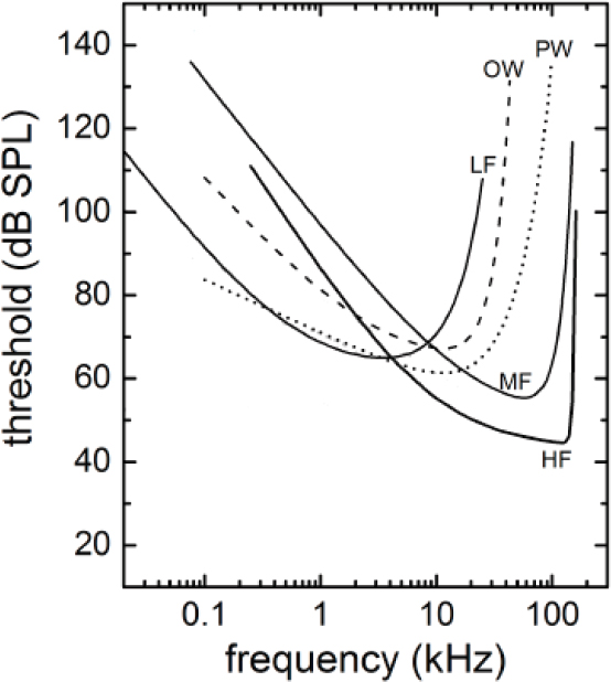
Studying what sounds cause masking or TTS demands understanding how the sensitivity of hearing varies with frequency, which is achieved by measuring audiograms of different species. It has become apparent from studies on marine mammal hearing that their auditory capabilities differ considerably among species. Underwater audiograms have been determined using either behavioral or physiological methods for 18 species of cetaceans (14 in the mid-frequency hearing group, 4 in the high-frequency hearing group, and none for baleen whales) and 11 species of pinnipeds and other marine carnivores (6 phocids and 5 in the combined otariids, sea otters, and walrus) (Mooney et al., 2012; Finneran, 2016). Behaviorally determined audiograms are available for individuals from four of the five marine mammal groups (mid- and high-frequency cetaceans and phocids and otariids in water). Within each group, the audiograms were combined to arrive at a best-fit composite audiogram for that group as shown in Figure 2.2. No hearing measurements have been made on low-frequency cetaceans. Hence the estimated hearing thresholds were calculated based on data from Cranford and Krysl (2015), Houser et al. (2001), Parks et al. (2007a), and Tubelli et al. (2012) as described by Finneran (2016).

The curves for all hearing groups follow a typical mammalian pattern in which there is a best frequency of hearing. Below the best frequency there is a gradual falloff in hearing sensitivity for low frequencies and above there is a much more rapid falloff in hearing sensitivity for high frequencies. These curves represent the best available peer-reviewed data. It is recognized that the curves are based on small numbers of animals, and only a few species are surrogates for each entire hearing group. No data were available for low-frequency cetaceans, so this estimate is based on correlation and assumptions.

Finding 2.3: A behavioral dose–response relationship can be determined without knowing the subject’s audiogram. However, understanding the physiological effects of sound from TTS through PTS requires an audiogram. For baleen whales physiological sound impacts are estimated based on modeling of the skull, estimated historical ocean noise thresholds, and data from other cetacean hearing groups. An audiogram from at least one species of baleen whale would be beneficial in understanding the effects of anthropogenic sound on baleen whales.

Permanent and Temporary Threshold Shift

If sounds are loud enough, they can lead to TTS. As indicated by the name, the hearing threshold returns to baseline in minutes to hours after the cessation of the stimulus, depending on the amount of TTS. The energy in the sound that generates a TTS is expressed as the SEL and measured in dB re 1μPa²-s. TTS and the growth in TTS with increasing SEL have been measured in four cetacean and three pinniped species. The weighted TTS threshold ranged from 153 dB_SEL for high-frequency (HF) cetaceans to 193 dB_SEL for otariids in water (Finneran, 2016). TTS can reduce an animal’s communication space and its abilities to detect predator and prey during the minutes to hours it takes for the threshold to return to its preexposure state. It is arguable whether this temporary reduction in hearing sensitivity represents an injury in itself. Kujawa and Liberman (2006) demonstrated in laboratory mice that noise exposures that cause only TTS may cause pathological changes that render the auditory system more vulnerable to age-related hearing loss. However, TTS is not considered an injury in the U.S. regulatory framework. No experiments have investigated the long-term effects of TTS in marine mammals, or have tried to create a PTS in a marine mammal (but see Kastak et al., 2008). Based on data from terrestrial mammals, the onset of PTS has been set by Southall et al. (2007) at an SEL that would produce 40 dB of TTS. Thresholds for PTS can then be calculated by knowing the threshold for onset of TTS and estimating the growth in TTS with increasing sound levels. For impulsive sounds, TTS in laboratory animals increases with a slope of 2.3 dB of TTS per dB of noise, suggesting a minimum of 15 dB SEL above TTS onset for PTS caused by impulsive sound. Similarly the slope for nonimpulsive sounds, based on human data, is 1.6 dB of TTS per dB of noise or conservatively rounded down to 20 dB SEL above TTS onset for PTS (Southall et al., 2007). The amount of sound energy required to produce injury based on TTS data has been summarized by Southall et al. (2007) and the NMFS (2016a) for each of the marine mammal hearing groups. The HF cetaceans have the lowest estimated PTS threshold, 173 dB_SEL for nonimpulse sounds, but the predicted range of injury is not necessarily much less than for the higher thresholds at lower frequencies, because lower frequencies propagate better than higher frequencies. The sound energy required to cause injury judged by PTS is so great that zones of injury for even intense sound sources such as airguns and naval sonars are estimated at

less than 1 km for all but a few cases. For example, a single one-second ping from one of the loudest naval sonars, the 53C, would be above the PTS threshold for HF cetaceans out to a range of 1 km given omnidirectional propagation, while it would be above the PTS threshold for mid-frequency and low-frequency cetaceans for less than 100 m from the source. These ranges suggested monitoring and mitigation measures that focused on detecting animals close to the source ship and suggest that the probability of marine mammals experiencing PTS from anthropogenic activities will likely be sufficiently low as to preclude any population-level effects.

Finding 2.4: Studies of noise levels that cause TTS and the growth in TTS with increasing noise are used to predict the occurrence of permanent hearing loss. Currently data exist for one species of otariid, two species of phocids, two species of mid-frequency (delphinid) cetaceans, and two species of high-frequency (phocoenid) cetaceans. Only a few individuals (one to five) of each species have been tested and within hearing groups there is wide variation in TTS onset and growth with increasing levels of noise. This variation indicates that the physiological effects of sound cannot be generalized based on testing of a few species of marine mammals, and more species need to be studied.

Behavioral Responses

Just about the time that data from TTS studies started to suggest limits on the ranges at which sound could injure marine mammals, evidence began to accumulate that lethal strandings of a poorly known group of whales called beaked whales coincided with naval sonar exercises. Frantzis (1998) described an atypical mass stranding where 12 Cuvier’s beaked whales (Ziphius cavirostris) stranded over 38 km of a Greek bay over 2 days when a naval sonar was being tested. Issues with mid-frequency sonar came to national attention in the United States following the stranding of 17 cetaceans and the death of 7 during a naval sonar exercise on March 15-16, 2000, in the Northeast and Northwest Providence Channels of the Bahamas Islands. A joint U.S. Navy and U.S. Department of Commerce report (Evans and England, 2001) determined that “the cause of this stranding event was the confluence of the Navy tactical mid-range frequency sonar and the contributory factors . . . a strong surface duct, unusual underwater bathymetry, intensive active use of multiple sonar units over an extended period of time, a constricted channel with limited egress, and the presence of beaked whales that appear to be sensitive to the frequencies produced by these sonars.” Usually when whales mass strand, they strand together at the same time. D’Amico et al. (2009) cataloged 12 atypical mass strandings of beaked whales that coincided with naval exercises that may have transmitted sonar. These strandings represent the most obvious and clearly lethal impact of anthropogenic sound on marine mammals.

Cox et al. (2006) reported on a workshop convened by the U.S. Marine Mammal Commission in 2004 to synthesize the current understanding of beaked whale strandings and to recommend research initiatives to determine the most probable causal pathways between transmission of mid-frequency sonar and strandings of beaked whales. The consensus from that meeting, which has not changed to date, was that a behavioral response occurring under a combination of contributory conditions was the progenitor of the strandings and the associated pathologies. Extensive behavioral, physiological, and anatomical research has been conducted over the last decade and a half to better understand not only this extreme example of the effect of anthropogenic sound on marine mammals but that of less dramatic chronic and episodic exposures. Some of the beaked whales that stranded during sonar exercises showed gas and fat emboli apparently caused by a decompression sickness (DCS) (Jepson et al., 2003; Fernández et al., 2005). Fernández et al. (2012) reported on three beaked whales that appear to have died at sea from decompression symptoms and then washed ashore, suggesting that whales do not just die from stranding, but may die directly from DCS at sea. These results have reinvigorated analysis of the diving physiology of deep-diving whales to better understand how they manage N₂ and other gases under hydrostatic pressure (Hooker et al., 2012). Current thinking is that anthropogenic noise can in some situations trigger behavioral reactions that may interfere with the ways whales manage gas under pressure and/or may cause whales to strand and die.

Dose–Response Relationships

This understanding that sound can trigger behavioral responses that may lead to injury or death motivated research to better define the relationship between exposure to sound and behavioral responses that could lead to effects that regulators view as “Level B takes” under the U.S. Marine Mammal Protection Act. Managing the impacts of underwater sound requires an understanding of the effect of this disturbance on individuals and the risk to the population. Dose–response relationships have commonly been used in toxicology to relate the level of exposure to the probability of a particular response or to the elicitation of different responses with differing levels of severity. When we discuss the first case, we will call these dose–p(response) relationships, and when we discuss the latter, we will call these dose–s(response) relationships. Toxicologists typically study genetically inbred laboratory animals under conditions designed to minimize stress, narrow the diversity of subjects, and control all variables except the experimental one to provide the strongest baseline condition for experimental detection of effects of known dosages of a single stressor. Behavioral responses of marine mammals are highly context dependent, being influenced by age (Houser et al., 2013a), sex (Symons et al., 2014), behavioral state (Sivle et al., 2012; Goldbogen et al., 2013), location (Tyack and Clark, 1998),

prior exposure resulting in habituation (Houser et al., 2013b) or sensitization (Kastelein et al., 2011), and individual sensitivities. Most experimental studies on the effects of an anthropogenic sound stimulus on marine mammals have been conducted with subjects drawn from wild populations. If the subjects are a representative sample of the contexts that affect responses, then the dose–response functions and other behavioral observations should be appropriate for the populations under study. Behavioral dose–response functions for three species were obtained from captive animals, and all TTS research has been done with captive animals.

One approach to estimating dose–response functions assumes a specific functional relationship between exposure and response. Many methods to estimate dose–response functions often assume a sigmoidal shape with a monotonic relationship between exposure and response. Some toxicological dose–response curves do not have this functional form (Calabrese, 2005), and we cannot assume that behavioral responses to sound will have a sigmoidal shape. Most dose–p(response) analyses assume a minimum exposure below which no response is expected and a maximum exposure above which all of the animals are assumed to respond. In the case of behavioral responses to sound, the minimum exposure can be assumed to occur at the limits of detectability as determined by the frequency-dependent audiograms. Ellison et al. (2011) emphasize the importance of context and environment in modulating the behavioral response to a given received level. Context includes current behavioral state and past exposure to the signal, and environment includes all the environmental factors that influence the signal-to-noise ratio and may result in a masked response threshold. DeRuiter et al. (2013) provided evidence that animals are more likely to show a response to a nearby signal at lower intensity than they do to a signal coming from farther away but with a greater received level. For example, tagged Cuvier’s beaked whales responded to the simulated sonar at received levels as low as 89 dB re 1 μPa but did not respond to sonar from an active naval ship farther away with a received level up to 106 dB.

Within the U.S. regulatory structure, Level A takes (injury) are equated with exposures resulting in PTS, whereas both TTS and behavioral disruption are regarded as Level B takes. Level B behavioral takes are generally considered to be less severe than Level B physiological takes (TTS). It is likely that, at the maximum exposure for behavioral response, animals may already be experiencing TTS. Note that in the case of the beaked whale strandings, exposures well below those required for PTS did disrupt behavior in a way that led to the death of the animals that stranded, so the logic of this regulatory structure is questionable for some settings.

The importance of understanding how sonar initiates a behavioral response in cetaceans has been the impetus to several studies that have developed empirical dose–p(response) curves linking the probability of a behavioral response to a given sound exposure. Finneran and Jenkins (2012) constructed a behavioral response curve that is used by the U.S. Navy and its regulator to estimate the proportion of animals receiving a given sound level that will show the criterion behavioral response. The Finneran and Jenkins (2012) curve is based on a mathematical formula following Feller (1968) and based on data from Finneran and Schlundt (2004), Fromm (2009), and Nowacek et al. (2004). The threshold response level is set at 120 dB_RMS and the level at which the probability of response is 0.5 is at 165 dB_RMS, resulting in an asymptotic value of approximately 200 dB_RMS for 100% response.

Another approach used to estimate probabilistic dose–p(response) functions assumes that the distribution of the probability of responses as a function of exposure is Gaussian (truncated at a lower and upper SEL) and estimates the mean and variance for this relationship (Antunes et al., 2014; Miller et al., 2014). Hierarchical Bayesian models can be used to estimate dose–p(response) functions, assuming that each individual has a response threshold, and that the distribution of thresholds across the population is (truncated)

normal. Observed levels associated with responses are then used to estimate the population mean and variance, which together with the minimum and maximum values can be used to estimate the dose–p(response) function.

Figure 1a in Box 2.2 shows the dose–p(response) function for killer whales exposed to 1-2 kHz and 6-7 kHz sonar, where the 50% response was at 141 ± 15 dB_RMS with thresholds ranging from 94 to 164 dB (Miller et al., 2014). Similar dose–p(response) functions have been determined for exposure to sonar for Blainville’s beaked whale (RL_p50 at 150 dB_RMS; Moretti et al., 2014), long-finned pilot whales (RL_p50 at approximately 170 dB_RMS; Antunes et al. 2014), a captive harbor porpoise (RL_p50 at 124-144 dB_RMS depending on sonar type; Kastelein et al., 2013), captive bottlenose dolphins (RL_p50 at 162 dB_RMS on first trial and 174 dB_RMS by tenth trial; Houser et al., 2013b), and captive California sea lions (RL_p50 at 147 dB_RMS increasing to 158 dB_RMS when sensitive juveniles [<2 years] were removed; Houser et al., 2013a). The responses used to establish the response function varied: presence or absence of a foraging dive in a 30-minute period for Blainville’s beaked whale where the stimulus was actual naval sonar operations; a change in two-dimensional movement tracks for long-finned pilot whales where the stimulus was simulated sonar in a controlled exposure experiment (CEE); an avoidance reaction as determined by an expert group consensus for killer whales where the stimulus was simulated sonar in a CEE; a sudden change in swimming speed or direction for the captive harbor porpoise where the stimulus was synthesized sonar signals; and primarily based on a statistically significant change in breathing during a 30-second period for captive bottlenose dolphins and California sea lions where the stimulus was simulated sonar. These studies have generally been based on relatively small sample sizes, in some cases a single animal, but have indicated that the responses are dissimilar enough that taxonspecific rather than a generic odontocete exposure–response relationship is necessary for impact assessments (Antunes et al., 2014; Harris et al., 2015). The responses of captive bottlenose dolphins also suggested that they may be capable of habituation to repeated exposures (Houser et al., 2013b), in contrast to California sea lions that did not demonstrate habituation under a similar experimental protocol (Houser et al., 2013a). This does not mean that pinnipeds do not habituate to sounds under other circumstances, but simply that they did not show habituation under this experimental protocol.

The responses used to establish the above-referenced dose–p(response) functions have varied in severity and most of them would be considered minor on the 10-point severity scale presented by Southall et al. (2007). The responses noted above range in severity from 2 (brief or minor changes in respiration rate) for captive bottlenose dolphins and California sea lions, to 3 (minor changes in locomotion speed, direction, and/or dive profile but no avoidance of sound source) for captive harbor porpoises and long-finned pilot whales, to 4 (moderate changes in locomotion speed, direction, and/or dive profile but no avoidance of sound source) for Blainville’s beaked whale, to 6 (minor avoidance of sound source) for killer whales. These experiments are designed so as not to harm the subjects. In this sense the experiments have succeeded, but it may take some extrapolation to predict thresholds for more severe responses if those are more relevant for a specific regulatory regime. Miller et al. (2012a) reviewed data from dose–s(response) experiments on killer, long-finned pilot, and sperm whales and reported that there was no consistent relationship between exposure and the severity score assigned to a response. It was noted that just-audible signals could result in responses of severity levels between 0 and 7. This variation highlights how different the responses of different individuals may be to similar acoustic levels of exposure. Ellison et al. (2011) suggest that contextual factors cause variability in responsiveness at low received levels, but annoyance/disturbance responses may be evoked in most animals over a relatively narrow range of high levels of acoustic exposure. This argues against assuming that the distribution of responses is likely to fit a symmetric normal distribution around a mean, but might better be viewed as a hybrid of several distributions driven by different processes.

Harris et al. (2015) demonstrated when combined killer whale, sperm whale, and long-finned pilot whale dose–p(response) data were plotted for three different levels of severity of response, a basically sigmoidal curve was generated for each severity level. For low severity of response, the curve reached 0.5 response probability at 153 dB_SEL and asymptoted at 1.0 probability at 167 dB_SEL. For medium severity of response, the curve reached 0.5 response probability at 155 dB_SEL and reached 1.0 probability at 180 dB_SEL. For the highest severity of response, the curve asymptoted at a 0.1 probability of response at 160 dB_SEL. The overall population effect will be a function of the probability of a response and the severity of the response. It is not yet possible to determine whether a greater probability of a less severe response or a lower probability of a more severe response will have the greatest population consequences.

Dose–p(response) relationships have not been estimated for the same marine mammal species in both captive and natural settings, but limited data suggest different responsiveness across these contexts, albeit using different criteria for the response. A free-ranging bottlenose dolphin tagged before the start of naval sonar exercises remained in the same general area during the 3 days of exercises and had modeled exposure levels up to 168 dB_RMS (Baird et al., 2014). This value is above the RL_p50 for captive dolphins on the first trial at an exposure SPL of 162 dB_RMS. The response of free-ranging harbor porpoises to a commercial two-dimensional seismic airgun survey in the North Sea was determined through passive acoustic tracking. The density of porpoises was unchanged at 10 km at received SPL of 148 dB_RMS and reduced by 6% at 5 km at received levels of 155 dB_RMS (Thompson et al., 2013a). These levels are well above the RL_p50 estimated for a captive harbor porpoise exposed to sonar (124-144 dB_RMS),

although another captive harbor porpoise consistently exhibited an aversive behavioral reaction to seismic airgun sound at SPL above 174 dB_RMS (Lucke et al., 2009). Captive studies have provided necessary first-order information on dose–response relationships for species too small or too difficult to tag under current methods, but they are an inadequate proxy for dose–response relationships determined in free-ranging animals because the context is so different, and the suite of behavioral responses available to captive animals is restricted compared to that available to free-ranging animals. This lack of dose–response data is particularly important for small pelagic odontocetes that form the majority of animals predicted to be taken in many environmental assessments (e.g., U.S. Department of the Navy, 2013). The responses observed in captivity are also low on the severity scale and would be unlikely to have population consequences in the wild.

Finding 2.5: The selected response criterion for dose–response studies has typically been a low-severity response, but anomalous high-severity responses have been observed during these studies. Just-audible signals have resulted in responses of severity levels between 0 and 7. The severity levels were established based on assumed effects on individual fitness, and thus severe responses to low sound levels raise concerns regarding population consequences.

Finding 2.6: A primary reason for having no free-ranging dose–response curves for any of the smaller cetaceans is the lack of a suitable data recording package for attachment to these animals. The development of such a data recording package that would combine GPS with a measurement of sound exposure level is essential to estimate the impact of sound on these species that constitute the vast majority of cetaceans exposed to anthropogenic sound.

Many species of marine mammals continue to occupy U.S. naval test and training ranges in Southern California, the Bahamas, and Hawaii (Falcone et al., 2009; McCarthy et al., 2011; and Baird et al., 2014, respectively). These range animals have been observed to respond to sonar activities with changes in diving patterns and movements. For example, Blainville’s beaked whales move to the periphery of the U.S. Navy’s Atlantic Undersea Test and Evaluation Center (AUTEC) range during training exercises with multiple ships operating sonar. They return to the range within a few days after the training exercises have concluded (McCarthy et al., 2011; Tyack et al., 2011). It is very difficult for observational studies to demonstrate that sonar is the cause of these reactions (see Chapter 6). A combination of controlled experiments to demonstrate causation, with opportunistic observations of actual exercises to study the scale and significance of responses (Tyack et al., 2011), has proven particularly informative. The long-term consequences of the energetic costs of displacement and changes in foraging location and potential changes in foraging resources are not completely known, but a recent study (Claridge, 2013) has shown that the average animal abundance of beaked whales at AUTEC is lower than in an equivalent area at Abaco, an area 170 km away in the Bahamas where sonar exposure is limited. Also the female-to-calf ratio at AUTEC is higher, suggesting lower recruitment. Beaked whales have both capital and income breeding characteristics (Huang et al., 2011). New et al. (2013b) developed an energetic model that considered the impact of displacement from food resources on survival and reproduction of beaked whales. Their results showed that, while adult survival was relatively robust under reduced energy input, minor reduction in energy intake over an extended period could affect lifetime reproductive output.

Killer whales represent an existential threat to marine mammals of several species, so playback of killer whale calls has been used as a positive control in studies of responses to anthropogenic sound. Blainville’s beaked whales (Tyack et al., 2011) and gray whales (Malme et al., 1983) show behavioral responses to playbacks of killer whale vocalizations when the signal-to-noise ratio is 0 dB. Some cetaceans also respond to some anthropogenic sounds, such as sonar at levels well below the current criteria for disturbance used in the United States. The 50% probability of a startle response for a captive harbor porpoise to playback of 6-7 kHz up-sweeps mimicking naval sonar signals occurred at SPL received levels of 101 dB_RMS (Kastelein et al., 2012). The minimum level for response of Cuvier’s beaked whales to playback of sonar signals occurred at SPL received levels of 89-127 dB_RMS, although the whales did not respond to sonar from a distant warship at received SPL of 78-106 dB_RMS (deRuiter et al., 2013). The above data show that the thresholds defining behavioral harrasment used by NMFS (160 dB_RMS impulsive sounds; 120 dB_RMS nonimpulsive) need to be updated in light of the new data for sonar. Some harbor porpoises and Cuvier’s beaked whales respond at levels well below the 120 and 140 dB_RMS response thresholds currently used for these species. Similarly, the 50% probabilities of response are in most cases below the 165 dB_RMS previously used in environmental impact assessments for naval activities. As described in Box 2.2, the current method of calculating takes based on response thresholds can lead to an underestimate of the number of animals taken.

Masking

With behavioral responses being observed at dose levels close to the limits of detectability in some cases, and with detectability used to set the minimum exposure at which the dose–response function starts, the acoustic signal-to-noise ratio needs to be considered when it limits detectability through masking. Masking occurs when the level of detectability for one sound is increased in the presence of a second sound by an amount expressed in dB. The mammalian ear

has been modeled as a bank of overlapping band-pass filters⁸ and only energy in the band-pass filter centered on the sound being detected, the critical band, contributes to the masking of that sound (Fletcher, 1940). While this has been investigated most thoroughly for Gaussian⁹ noise, it does not hold true for many natural and anthropogenic noises that have complex spectra and amplitude fluctuations. Through a phenomenon known as comodulation masking release (Trickey et al., 2010), the broader the frequency band of the natural noise is outside the critical band, the more the masking is reduced compared to what it would have been with Gaussian noise in the critical band. Masking has been considered primarily in the case where the second sound represents noise for the species or individual in question. For example, concern has been expressed that shipping noise, which has increased since the advent of motorized vessels, overlaps with the frequency range of important social calls of baleen whales, including blue (Mellinger and Clark, 2003), fin (Watkins et al., 1987), and right (Parks et al., 2007a) whales. The primary concern here has been that elevated ambient noise would reduce the range over which whales could detect calls of conspecifics.

Clark et al. (2009) have proposed analyzing the potential effect of masking through a calculation of the reduction in communication space for several species of baleen whales. They found the most profound reductions due to the modeled passage of two ships within 4 km of a right whale in the Stellwagen Bank National Marine Sanctuary, where the aggregate exposure resulted in an 84% reduction in the communication space for that animal. Hatch et al. (2012) calculated an overall 63% reduction in communication space for right whales in Stellwagen Bank National Marine Sanctuary compared to what they experienced in the mid-20th century, when background levels were estimated to be 10 dB below the lowest 5% of all the background levels currently recorded.

One serious problem with these predictions is that they ignore compensation mechanisms that whales use to maintain the effective range of their communication signals in noise. The natural environment in which animal communication evolved has significant variation in noise, for example from rain (heavy rain causes up to a 40 dB increase) or waves and bubbles caused by wind (8 dB increase between Beaufort 0.5 and 1.0), and most birds and mammals have evolved mechanisms to compensate for this natural variation in noise. One of the most pervasive compensation mechanisms is the Lombard effect, by which animals increase the source level of their calls in increased noise (Brumm and Zollinger, 2011). All birds and mammals tested have shown the Lombard effect, and marine mammals are no exception. Killer whales increased their call amplitude by 1 dB for every dB increase in background noise created by motorized vessels (Holt et al., 2009). Making louder calls in increased noise can have an energetic cost; bottlenose dolphins increase their metabolic rate as the acoustic energy of their vocalizations increases (Holt et al., 2015). In the case of the right whales in Cape Cod Bay, the location modeled by Clark et al. (2009), Parks et al. (2010) showed that individual right whales elevate the source level of their calls as the noise level increases. In addition, as shipping noise chronically increased from the 1960s to the 1990s, right whales have increased the fundamental frequency of their calls by about an octave, outside of the peak frequency of shipping noise (Parks et al., 2007b). These mechanisms are not taken into account in the Clark et al. (2009) model, making it unrealistically extreme in its predictions of reduction of effective space. Other mechanisms by which human engineers compensate for noise include making signals longer and/or more redundant. These mechanisms are also used by marine mammals; humpback whales increased the duration of their songs by 29% in the presence of low-frequency active sonar, and this was produced by increasing the redundancy of the song (Miller et al., 2000).

In addition to potential effects on communication space, shipping can also act as a physiological stressor. Rolland et al. (2012) measured fecal glucocorticoids in North Atlantic right whales in the Bay of Fundy during the summers of 2001-2005. Shipping activity was reduced by 67% and the associated noise levels declined by about 6 dB immediately after the attack on the World Trade Center on September 11, 2001. This reduction in ship movement and noise was associated with a reduction in stress-related glucocorticoids compared to other years and before September 11, 2001. However, this opportunistic study lacked the controls required for standard experimental design.

Impulsive Sources

Impulsive sources affect animals differently than relatively continuous sources. The rise time and peak pressure (measured in kPa) are more important metrics than the root mean square (RMS) value of the received level. Depending on the interpulse interval, the auditory system may have an opportunity to partially recover between pulses. As noted previously, the current NMFS threshold for behavioral response to impulsive sounds is 160 dB_RMS and for nonimpulsive sounds it is 120 dB_RMS. The primary sources of impulsive sounds that marine mammals experience come from seismic activity associated with oil and gas exploration; pile driving associated with construction of bridges, docks, and wind farms; and some acoustic deterrent devices associated with fishing and aquaculture.

___________________

⁸ A band-pass filter allows a range of frequencies to pass with minimum attenuation and strongly attenuates frequencies outside that band. The width of the band-pass is typically given as the frequencies above and below the center frequency at which the attenuation is 3 dB.

⁹ Gaussian noise has a normal distribution of instantaneous amplitudes over time.

Seismic Surveys

Responses to seismic surveys have been studied in a variety of marine mammals. The following overview captures most of the salient results but is not a comprehensive literature review. Romano et al. (2004) sampled blood from a captive beluga whale (Delphinapterus leucas) and bottlenose dolphin (Tursiops truncatus) after exposure to underwater impulsive sounds from a seismic water gun. For the beluga whale, levels of norepinephrine, epinephrine, and dopamine were significantly higher for peak pressure levels of 116 to 198 kPa. For the dolphin, serum levels of aldosterone were significantly elevated and monocytes decreased after exposure to peak pressure levels of 146 to 220 kPa. Miller et al. (2009) conducted controlled approaches of a commercial seismic survey vessel to make pass-bys of sperm whales in the Gulf of Mexico. The whales, which were exposed to received levels varying from 120 to 147 dB_RMS at ranges varying from 1.4 to 12.8 km, did not change their direction of travel or behavioral state in response to exposure, but did decrease the energy they put into swimming and showed a trend for reduced foraging. Madsen et al. (2002) studied responses of sperm whales in Norwegian waters to seismic surveys at ranges greater than 20 km and reported no responses at exposure ranging up to 123-130 dB_RMS. Avoidance responses have more commonly been reported for baleen whales. Avoidance responses to airgun sounds at received levels of 160-170 dB_P-P re 1 μPa have been reported for migrating gray whales (Malme et al., 1983), bowhead whales (Richardson et al., 1986), and migrating humpback whales (McCauley et al., 2000). Fin whales moved away from a 10-day seismic survey in the Mediterranean and were spatially displaced for at least 14 days after the seismic airgun shooting period (Castellote et al., 2012). The survey area affected was estimated to be about 100,000 km² (Castellote et al., 2012).

Pile Driving

Pile driving is used in the construction of structures, such as piers and bridges, and the installation of oil and gas platforms and offshore wind turbines. The impact of pile driving for offshore wind turbines has been of particular concern for marine mammals because of the high source level (Madsen et al., 2006). Pile driving produces broadband, multiple pulsed sounds, similar to seismic airgun surveys, with the peak energy below 1 kHz (Bailey et al., 2010). During pile driving, hammer strikes occur about every 1-2 seconds and the piling duration is generally several hours for each pile with the interval between piles varying from minutes to days (Bailey et al., 2010; Dähne et al., 2013). Source levels vary depending on the size of the pile and method of pile driving, but have been estimated to be 226-257 dB_P-P re 1 µPa at 1 m based on recorded levels back-calculated to 1 m (OSPAR, 2009; Bailey et al., 2010). Sound levels of 205 dB_P-P at 100 m (Bailey et al., 2010) and energy up to 176 dB_SEL re 1 µPa²-s at 720-750 m distance (Brandt et al., 2011; Dähne et al., 2013) have been reported.

In Europe, assessments of the impacts of offshore wind developments on marine mammals have focused on small cetaceans and pinnipeds (Bailey et al., 2014). The response of marine animals to the construction phase, particularly the pile-driving activity, has primarily been studied for the most abundant cetacean species in the North Sea, the harbor porpoise (Phocoena phocoena). Harbor porpoises have been reported to exhibit an avoidance response to the impulsive sound of pile driving at distances of 20 km or more and for up to 3 days (Tougaard et al., 2009; Thompson et al., 2010; Brandt et al., 2011). There is currently a lack of data for large whales. Large whales are classified as having low-frequency hearing (see Figure 2.2), which suggests that they may be most sensitive to pile-driving sounds. Offshore wind energy areas have been identified and leased by the Bureau of Ocean Energy Management on the U.S. Outer Continental Shelf where a number of whale species, many of which are listed as endangered species, are known to occur. As offshore wind energy facilities begin to be installed off the U.S. coast, studies on the short- and long-term responses of large whales will be particularly important for determining the potential population-level consequences.

Acoustic Deterrent Devices

Acoustic deterrent devices (ADDs) are intentionally designed to deter wildlife such as marine mammals from depredating resources such as fish in a fish farm. A variety of different ADDs have been developed to deter seals from depredating fish farms (reviewed by Nowacek et al., 2007; Götz and Janik, 2013). Götz and Janik (2013) reviewed mixed evidence on the effectiveness of ADDs in reducing depredation by seals. Activation of ADDs in some settings was associated with increased depredation, perhaps through broadcasting the location of a food source (Geiger and Jeffries, 1987; Jefferson and Curry, 1996). In other settings, ADDs were judged by fish farmers to vary from ineffective to moderate effectiveness in different sites (Quick et al., 2004; Sepulveda and Oliva, 2005). In cases where ADDs were associated with reduced depredation, some showed a decreased effect over time, which could be due to habituation (Groves and Thompson, 1970), tolerance (Bejder et al., 2009), or hearing damage due to exposure to the ADDs (Reeves et al., 1996).

In contrast to the mixed evidence for effectiveness of ADDs on the target pinnipeds, there is strong evidence that operation of ADDs causes some odontocetes to avoid large areas of habitat. Morton and Symonds (2002) studied the presence of killer whales in inshore waters of British Columbia where their distribution had been well studied for more than a decade before four ADDs were installed. Sightings of killer whales were significantly reduced in

the roughly 10 km² area where the ADDs were installed during the 6-year period of their use, and then recovered to baseline after their use ended. Olesiuk et al. (2002) report a similar sharp decline in sightings of harbor porpoise out to their maximum sighting range of 3.5 km when ADDs were activated for periods of 3 weeks. Brandt et al. (2013) showed a similar decrease in the abundance of porpoises detected out to ranges of 7.5 km from an ADD when it was operating. None of these studies suggest much habitation in the response of odontocetes to ADD signals.

INDIRECT EFFECTS OF SOUND ON MARINE MAMMALS

Marine mammals are among the animals with the most sensitive underwater hearing, but sound may also affect them indirectly through effects on prey, predators, or competitors. Indirect effects of stressors may be more important than direct ones (Ockendon et al., 2014).

Effects on Prey

Some fish are specialized to hear the pressure component of sound. A few species of herring (subfamily Alosinae) can detect the ultrasonic clicks that toothed whales use to find their prey. Wilson et al. (2011) demonstrated that one of these species swims away from these clicks, in a directional antipredator response. Mann et al. (1998) showed that shad respond to echolocation clicks at received levels of 171 dB_P-P. This level is high enough that few sources of noise would be likely to mask the clicks, so it is unlikely that elevated noise would make the shad less likely to escape. Most prey of marine mammals detect the particle motion component of sound rather than the pressure component. This mode of hearing limits the ability of animals to hear sounds with wavelengths smaller than roughly their body size, so these animals do not hear well above a few kilohertz. However, some low-frequency sources of anthropogenic sound, such as airguns used in seismic surveys, have been shown to affect the hearing and behavior of fish. McCauley et al. (2003) found that caged fish exposed to repeated passes of a seismic air gun (source level of 222.6 dB_P-P re 1 μPa at 1 m) starting 400-800 m away and passing within 5-15 m of the cage experienced significant hair cell damage that remained unresolved 58 days later. They note that, had the fish not been caged, they would have swum away as they tried to do within the confines of the cage at first hearing of the seismic gun. Engås et al. (1996) report that the catch of cod and haddock was reduced by 50% when airguns began to transmit sound. Reductions in catch were observed 33 km away from the survey and lasted more than 5 days after the airguns stopped operating. The acoustic density of cod and haddock was reduced by 45% during the seismic survey and by 64% post survey. In contrast Løkkeborg et al. (2012) found that gillnet fisheries yields increased during a seismic survey while longline fisheries yields decreased. Acoustic mapping of fish abundance showed only pollock were displaced from the fishing grounds in this study. Løkkeborg et al. (2012) note that the airgun discharge rate was 19 times higher in the Engås et al. (1996) study, and they point out that the lower levels of exposure could explain the lower level of response in their study. If avoidance behavior reduces the prey of marine mammals, it could affect their feeding even if the sound does not affect them directly. However, short-term displacement of prey may have few consequences for marine mammals. Prey often move considerable distances for a variety of reasons, and presumably marine mammals can usually move to relocate them.

There is evidence that continuous noise, similar to the sound of shipping, may increase the mortality of eggs and larvae of a minnow (Cyprinodon variegatus; Banner and Hyatt, 1973) and decrease the growth of larvae of the minnow and longnose killifish (Fundulus similis). Regnault and Lagardère (1983) showed that exposure to noise 30 dB above ambient increased the metabolic rate of the shrimp Crangon crangon in an aquarium, with a significant reduction in growth and reproduction and elevated mortality (Lagardère, 1982). If chronic exposure to noise reduces the abundance of fish and invertebrate prey of marine mammals, this could reduce the quality of their habitats, resulting in site abandonment or survival and reproductive costs for individuals that remain.

Effects on Predators

Sharks and killer whales are some of the primary predators of marine mammals. Sharks do not have particularly sensitive hearing, so effects of noise are likely to be minimal. However, killer whales not only have excellent hearing, but have also been shown to be more responsive to low- and mid-frequency sonar than some other toothed whales, such as sperm and pilot whales (Harris et al., 2015). If killer whales avoid noise sources at greater ranges than potential prey, this could create a zone near the noise source with a lower risk of predation. Noise-mediated predator shelters or shields have been documented in terrestrial systems where songbird nest predators appear to be more sensitive to chronic noise than are their prey (Francis et al., 2009). In the same system, Francis et al. (2012b) found evidence of additional indirect effects with potential long-lasting consequences for the ecosystem. Specifically, the reduced recruitment of piñon pine (Pinus edulis), a foundational species, in noisy areas is linked to avoidance of noisy areas by a key seed disperser, the Woodhouse’s scrub-jay (Aphelocoma woodhouseii), and increased abundance of important seed predators. These studies highlight how noise, like other anthropogenic stressors, can have indirect effects that reverberate throughout communities by interfering with interactions among species. Given the many pathways by which anthropogenic noise could affect marine mammals, a potential benefit from a

predator shield must be weighed against potential costs of persisting in noise-exposed zones.

Effects on Conspecifics

Different kinds of noise can have varying effects on social cohesion in different species. Buckstaff (2004) showed that, as a motorboat approaches a group of bottlenose dolphins (Tursiops truncatus), the dolphins will increase the rate at which they produce signature whistles, followed by increased social cohesion (Nowacek et al., 2001). When sonar signals trigger a flight reaction, this can interfere with normal social cohesion, leading to separation of members of a group. For example, Miller et al. (2012a) report on a group of killer whales exposed to a playback of mid-frequency sonar sounds. When the received level of these sounds reached 152 dB_RMS, a calf that had been in the group was seen to have separated from the group. Miller et al. (2011) notes three unique characteristics of this experiment to this exposure session: it was the only repeated mid-frequency active sonar up-sweep exposure presented to the same group of animals; the experiment was conducted in an unusually narrow fjord roughly 1 km wide; and transmissions were started unusually close to the subjects. The calf rejoined the group after 86 minutes, and remained with the group for many hours after exposure. However, this separation was scored as quite a severe response because it could have had more serious consequences for the calf. High-latitude adult male sperm whales that are usually solitary responded to playback of killer whale vocalizations by clustering together at the surface and producing social alerting sounds (Curé et al., 2013).

RECOMMENDATIONS

Recommendation 2.1: Additional research will be necessary to establish the probabilistic relationships between exposure to sound, contextual factors, and severity of response.

Recommendation 2.2: Uncertainties about animal densities, sound propagation, and effects should be translated into uncertainty on take estimates, for example, through stochastic simulation. Regulators may then choose the level of risk they wish to use in deciding whether to permit an activity.