
3
Socioeconomic Outcomes of Immigrants
3.1 INTRODUCTION
The skill mix of the immigrant population—and, particularly, how their education and experience levels compare to those of the native-born—is a key determinant of the impact their arrival will have on the wages and employment in receiving labor markets. These characteristics also affect immigrant assimilation and immigrants’ fiscal impact. If an inflow of immigrants is composed mainly of low-skilled workers, it is reasonable to expect that the pre-existing low-skilled population (both native-born and earlier immigrant arrivals) will be most affected by the increased supply of workers. Likewise, if an immigrant inflow is composed of high-skilled workers in very specialized fields, pre-existing workers in those narrow fields are most likely to be affected.1 Furthermore, the skill mix of the immigrant population is likely to influence the speed with which immigrants assimilate in their new country. Skilled immigrants may acquire new skills more quickly, including English language fluency, and may have more ready access to job information that would allow them to catch up with natives relatively quickly.
Labor market skills are also directly linked to fiscal impacts. As with the native-born, low-skilled immigrants contribute less on average than their higher skilled counterparts to the public coffers in the form of income taxes and other kinds of taxes. Based on their lower incomes, on average,
___________________
1 In-depth theoretical and empirical support for these assertions comprise the content of Chapters 4 and 5.
they have greater eligibility for some programs. However, their immigrant status, even if legal, may make them ineligible for other programs.
Immigration confers economic benefits on the native-born population as a whole but, among the native-born, there are likely to be winners and losers. While pre-existing workers most similar to immigrants may experience lower wages or a lower employment rate, pre-existing workers who are complementary to immigrants are likely to benefit, as are native-born owners of capital. Beneficial effects of skilled immigration are likely to be reinforced in the presence of capital-skill complementarity, where native-owned capital becomes more productive when combined with high-skilled labor; the panel delves into these consequences of immigration in Chapters 4 and 5. These benefits may be further augmented if there are “productivity spillovers” between high-skilled immigrants and the native-born workforce.
This chapter summarizes trends in the skill mix of the immigrant population and addresses how these trends compare with those of natives. Educational attainment is examined, as are differences in the occupations of immigrants and the native-born. The chapter also examines the extent of economic assimilation: the rate at which the economic outcomes of immigrants catch up with those of native-born Americans, focusing on employment, wage, and English-language acquisition outcomes. It also reviews some of the differences between immigrants and the native-born in terms of poverty rates and participation in social assistance programs. The descriptive statistics presented here serve to link the discussion of context and history in Chapter 2 and the analyses of wage, employment, and fiscal impacts in later chapters.
3.2 EDUCATION AND OCCUPATION PROFILES
Education Profiles
Trends in the skills of immigrants relative to those of the native-born help answer questions such as whether today’s immigrants face greater or lesser barriers to full economic assimilation than in the past and whether they are likely to displace or complement native-born workers in certain segments of the labor market if they arrive in sufficiently large numbers. In this section, the panel examines changes in the distribution of educational attainment of immigrants over successive cohorts, relative to the corresponding native-born cohorts.
The education of a cohort of immigrants at a given point in time can be divided into two components: (1) the initial level of education they attained prior to their arrival in the United States, and (2) additional education attained after immigrating. Higher amounts of both are expected to lead to
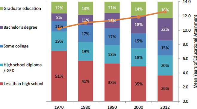
more favorable earnings outcomes and fiscal impacts. Using data from the 1970-2000 Decennial Census and the 2012 3-year American Community Survey (ACS),2 which covers the years 2010-2012, the panel documents how immigrants’ initial education upon arrival has changed over the past few decades. We define “recent immigrants” as persons who were born outside the United States (excluding those born to U.S.-citizen parents) who arrived within the 5 years prior to each census or to the 2012 ACS. The analysis is restricted to individuals ages 25 and older. Figure 3-1 shows that the education levels of immigrant cohorts upon arrival have been rising steadily over time. For example, about half of recent immigrants in 1970 had less than a high school education, but by 2012 this figure had halved to 26 percent. Whereas in 1970 only 20 percent of recent immigrants had completed postsecondary education (8% with college education and 12% with advanced education), by 2012 this proportion had increased to 38 percent (22% with college education and 16% with advanced education). Average years of school completed are superimposed on the same chart to reveal the steady upward trend, from 10.2 in 1970 to 12.6 in 2012.3
Section 3.6 of this chapter is a Technical Annex of the panel’s detailed tabulations and regression analyses based on Decennial Census and survey data in the Integrated Public Use Microdata Series (IPUMS). Tables 3-16 and 3-17 in Section 3.6 break out the educational attainment levels at arrival for men and for women, respectively. These tabulations show that increases since 1970 in immigrant education levels at arrival have been large for both men and women.
The rise in immigrants’ initial education over successive immigrant cohorts should be interpreted within a broader U.S. context, in which improvement in educational attainment has been a general phenomenon
___________________
2 The ACS data were accessed through IPUMS (Ruggles et al., 2015), with all estimates weighted to be nationally representative. In tables and text throughout Chapter 3, 2012 is used as shorthand for 2010-2012.
3 The continuous measure of educational attainment is calculated by first assigning each person the number of years of completed education above kindergarten as reported in the detailed educational attainment variable educ in the ACS data provided by IPUMS. For categories of years of education, such as “Grades 1, 2, 3, or 4,” the midpoint is used (in this case, 2.5 years). For educational attainment reported by category, such as “associate’s degree,” or “bachelor’s degree,” we followed Jaeger (1997) in assigning years of educational attainment. However, for those reporting a doctoral degree, we assigned additional years of educational attainment (beyond that used by Jaeger) on the basis of data on the average time to completion of doctoral degrees in the United States from the National Science Foundation (see http://www.nsf.gov/statistics/infbrief/nsf06312/). In results not presented here, we used a different coding scheme for calculating continuous years of educational attainment, relying on the IPUMS educ variable, which presents broader educational attainment categories that are consistent across years. The average years of education resulting from this alternate coding scheme were very similar to those resulting from our original coding scheme, which is used in this report.
SOURCE: Analyses of 1970-2000 Decennial Census data and 2010-2012 American Community Survey data, accessed through the Integrated Public Use Microdata Series.
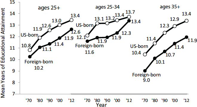
over birth cohorts in the native-born population (Fischer and Hout 2006). This comparison is important because, as noted in the introduction, the impact of immigration on wages and employment of the native-born is directly related to relative education (and experience) levels. Figure 3-2 compares trends in education (measured in mean years of schooling) for recent immigrants and for native-born persons. Given that about one-half of recent immigrants in each year fall in the 25-34 age range, compared to roughly one-quarter of native-born persons, Figure 3-2 presents the data separately for three age ranges: (1) everyone ages 25 and older, (2) those ages 25-34, and (3) those ages 35 and older.
The native-born have consistently higher educational attainment. However, for adults ages 25-35 (middle panel) there has been convergence in education between the two groups, particularly since the 1980s. In 1970, recent immigrants ages 25-34 had 0.5 years less schooling than their native counterparts, with mean levels of 12.1 for the native-born and 11.6 for a recently arrived immigrant. By 1980, the gap had expanded to 1.2 years, with mean education levels of 13.1 and 11.9 respectively. By 2012, the gap had narrowed to 0.3 years, with a mean of 13.7 years of education for the native-born and 13.4 for the recently arrived foreign-born. On the other hand, for the total ages 25 and older population (left-hand panel in
SOURCE: Analyses of 1970-2000 Decennial Census data and 2010-2012 American Community Survey data, accessed through the Integrated Public Use Microdata Series.
Figure 3-2), the educational gap between immigrants and natives ended up slightly larger in 2012 than in 1970 (0.8 versus 0.6 years of education) because, even as the native-born/foreign-born education gap narrowed for those ages 25-34, the gap remained steady for adults ages 35 and older, changing from 1.4 years of schooling in 1970 to a gap of 1.5 years in 2012.
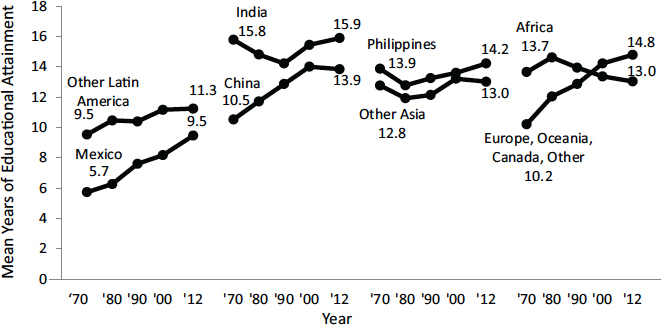
To assess trends for different groups based on national or regional origins, Figure 3-3 presents mean years of schooling among recent immigrants ages 25 or older across the largest immigrant groups identifiable in the data. The trends differ sharply by country or region of origin: The largest increases in educational attainment have occurred among immigrants from Mexico, China, and the group combining immigrants from Europe, Oceania, and Canada. Average Mexican immigrant education improved by 3.8 years, from a very low level of 5.7 years in 1970, to 9.5 years in 2012. Chinese immigrants started from a relatively high education level of 10.5 years and moved up to 13.9 years—an average increase of 3.4 years of schooling. For the miscellaneous group that includes immigrants from Europe, Oceania, and Canada, education levels increased over the analysis period from an average of 10.2 years of schooling to 14.8 years, for an average increase of 4.6 years. Immigrants from Latin American countries other than Mexico experienced an average increase of 1.8 years in edu-
SOURCE: Analyses of 1970-2000 Decennial Census data and 2010-2012 American Community Survey data, accessed through the Integrated Public Use Microdata Series.
cation levels from 9.5 to 11.3 years. Three origin groups—immigrants from India, Philippines, and Asia other than China—experienced a muted U-shaped profile, with very small net gains during the period. Immigrants from Africa are the only group with an opposite trend to that of all immigrants, as the average years of education of recent admission cohorts declined from 13.7 years in 1970 to 13.0 in 2012—but this group had a very high starting level.
Age-Education Pyramids
This subsection describes the age-education structure of the foreign-born and native-born populations in the United States. For the native-born population, the age structure is driven primarily by past fertility behavior and secondarily, in older ages, by mortality patterns. For the immigrant population, however, the age structure is determined less by fertility and mortality than by historical arrival rates and by the age composition of new immigrant inflows.
We use population pyramids to visualize the joint age-education structure of the foreign-born population relative to the native-born population from 1970 to 2002. Figure 3-4 presents an age-education pyramid for
foreign-born residents in 1970 and 2012. Figure 3-5 displays comparable information for native-born residents. These pyramids, like typical age-sex pyramids, graphically display the age distribution of a population. However, they differ from typical age-sex pyramids in two important respects. First, the pyramids do not reflect the actual sizes of the two populations, as they only show within-population proportions (i.e., each pyramid sums to 100 percent for its specified population); population sizes are provided in notes accompanying the figures. Second, each horizontal bar representing the relative size of an age group is divided into education groups—from low (light colored) to high (dark colored). Five education groups are distinguished for the population age 15 and greater: (1) less than high school (or less than 12 years of education, depending on the source data), (2) high school (12 years of education), (3) some college (13-15 years of education), (4) college completion (or 16 years of education), and (5) beyond college (more than 16 years of education).
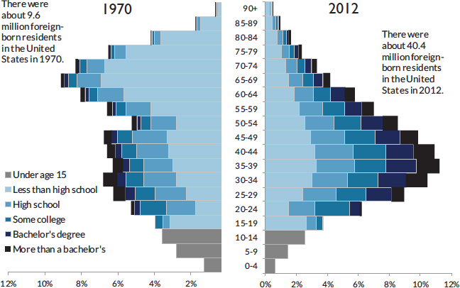
NOTE: The 9.6 million foreign-born U.S. residents in 1970 constituted 4.7% of the total population. The 40.4 million foreign-born U.S. residents in 2012 constituted 13% of the total population.
SOURCE: Analyses of 1970 Decennial Census data and 2012-2012 American Community Survey data, accessed through the Integrated Public Use Microdata Series.
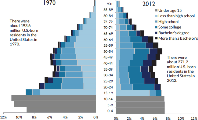
NOTE: The 193.6 million native-born U.S. residents in 1970 constituted 95.3% of the total population. The 271.2 million native-born U.S. residents in the United States in 2012 constituted 87% of the total population.
SOURCE: Analyses of 1970 Decennial Census data and 2012-2012 American Community Survey data, accessed through the Integrated Public Use Microdata Series.
Although the size of the native-born population increased during the observation period, the relative size of the total foreign-born population expanded much more. In 1970, the ratio of the native-born to the foreign-born population was about 20, meaning that there were 20 native-born U.S. residents for each foreign-born resident. This ratio steadily declined to 15 in 1980, 12 in 1990, 8 in 2000, and 7 in 2012.
Aside from children younger than age 15, the foreign-born population evolved from being a relatively old population in 1970 to a relatively young population in 2012. This is because most immigrants arrive in their early adult years (ages 20-35). A comparison of the two pyramids reveals that the number (and share) of immigrants ages 30-39 has swollen to offset the declining numbers of the native-born population in that age range, a decline due to the late 20th century fertility bust.
It is also noteworthy that in both 1970 and 2012 the educational attainment of the foreign-born population was more concentrated at the extremes than that of the native-born population, particularly for young
adults. In 1970, for example, 41 percent of the foreign-born population ages 30-34 had not completed high school, compared to 30 percent of the native-born. In the same age group, 11 percent of the foreign-born population had attained more than a 4-year college education in 1970, compared with 6 percent for the native-born population. By 2012, the percentage of the population ages 30-34 that completed less than high school was down to 29 percent for the foreign-born and to 8 percent for the native-born. At the high end of the education distribution, 13 percent of the foreign-born population had attained more than a 4-year college education, versus 11 percent of the native-born population. In 1970, for the 30-34 age group, 7 percent for the foreign-born population had 4-year college education (and no more) while 8 percent for the native-born population had 4-year college education (and no more). By 2012, the numbers at this achievement level had grown to just over 17 percent for the foreign-born population and almost 23 percent for the native-born population.
For the broader working age population—those ages 25-64—the relative differences in educational achievement between immigrants and natives are not dissimilar from those for the younger (ages 30-34) group. In 1970, 52 and 41 percent of the foreign-born and native-born populations, respectively, had not completed high school; by 2012, these rates had dropped to 28 and 8 percent, respectively. In this broader age group, 7 percent of the foreign-born population and 5 percent of the native-born population had attained more than a 4-year college education in 1970; these rates had climbed to just over 11 percent and just under 11 percent, respectively, by 2012. The percentage of the population in this age group with a 4-year college education (and no more) was slightly lower across the board relative to the 30-34-year-old cohorts: just over 7 percent for the foreign-born population and just over 8 percent for the native-born population in 1970; by 2012, the numbers at this achievement level had grown to just over 17 percent of the foreign-born population and just under 23 percent of the native-born population.
Three conclusions stem from comparing the education-age pyramids for natives and immigrants:
- Educational attainment of recent immigrants has improved appreciably over the past few decades.
- For recent immigrants ages 25-34, educational attainment has risen in comparison to that of native-born Americans. Among all age groups, however, the educational attainment gap has remained relatively constant over the period.
- Compared to the native-born, recent immigrants continue to be overrepresented among the high and low categories of educational attainment.
Occupation Profiles
As in most social surveys and statistical reports, U.S. Decennial Censuses and the ACS collect data on workers’ occupations by coding them into classification systems that delineate major differences in tasks performed and in the skills, education, or training needed across jobs.4 Detailed coding systems have evolved over time in response to changes in the occupational structure of the labor market. Tracking data on occupational changes over time requires a consistent coding system which, fortunately, has been created by Xie and Killewald (2012) and Xie et al. (2016). This system, based on classification of 41 occupational categories, was created to meet two conflicting objectives by (1) reducing the number of occupational categories and (2) grouping detailed occupations only when socioeconomic status and work content are sufficiently similar across these occupations.
The Technical Annex in Section 3.7 lists the occupational titles under each category for the 2000 Decennial Census. Table 3-18 in Section 3.6 presents the percentage shares of foreign-born male workers, from 1970 to 2012, within each occupational category. Table 3-19 does the same for female workers. In the last column of these tables, the share of workers with a bachelor’s degree or higher in 2012 is given as a measure of the socioeconomic status of the occupational category (Hauser and Warren, 1997).
Comparing the proportion of foreign-born workers within each occupation to the overall proportion of foreign-born workers across all occupations (top row in both Tables 3-18 and 3-19) reveals whether foreign-born workers are overrepresented or underrepresented in a given occupational category. One clear pattern that emerges for both men and women is that immigrants are concentrated in two types of occupations: (1) those requiring low levels of education, such as “cleaning service and food service workers,” “textile machine operators,” and “personal service workers and barbers,” and (2) professional occupations requiring high levels of education such as “physical scientists,” “life scientists,” “physicians, dentists, and related,” and “architects,” and “mathematicians.” Some occupations, such as “social and recreation workers,” “preschool and elementary teachers,” “protective service workers,” “secretaries,” and “bookkeepers,” have always had a low percentage of foreign-born workers. Changes in the share of foreign-born workers over time are most evident (in Tables 3-18 and 3-19) for “farmers and farm laborers,” “laborers, except farm,” and “computer specialists,” for which the share of foreign-born workers changed from underrepresentation to overrepresentation (relative to the foreign-born share of workers across all occupations). A change in the opposite
___________________
4 See http://www.bls.gov/soc/revising_the_standard_occupational_classification_2018.pdf [November 2016].
direction, from overrepresented to underrepresented, occurred for foreign-born workers occupied as “writers, artists, and media workers” and as “health technicians.”
Table 3-1 shows the results for male workers when the 41 occupational categories are collapsed into 8 major occupational categories (using the Tier 2 classification in the Section 3.7 annex on occupational classification). Table 3-2 shows the same for female workers. This level of classification reveals other dimensions of the patterns described above.
First, while foreign-born workers are overrepresented in high-level professional groups that require the most education (such as scientists, engineers, and architects), they are underrepresented among other professionals, managers, and sales personnel. This pattern probably reflects the differing importance of verbal communication skills in technical occupations versus those requiring interaction with customers and subordinates, as well as occupational licensing requirements in some professions. Also noteworthy is that growth over the 1970-2012 period in the share of foreign-born workers in the first four occupational categories listed in Tables 3-1 and 3-2 has been slower than the growth in the share of foreign-born workers in the general labor force (across all occupations), resulting in a relative decline of foreign-born workers in these higher-status occupations. For the next four lower-status occupational categories, increases are generally observed in the share of foreign-born workers that outpace the share of foreign-born workers across all occupations. As in the detailed occupational tabulations in Tables 3-18 and 3-19, the increase in foreign-born workers’ presence is most pronounced among “farmers and farm laborers,” growing from 2.7 percent of all male workers in that occupational category in 1970 to 26.9 percent in 2012 and from 3.8 percent of all female workers in the category to 32.6 percent.
The disproportionate share of foreign-born workers in both the highest- and lowest-skilled occupations may contribute to occupational segregation between foreign-born workers and native-born workers. To address this question, the panel computed the segregation index (Duncan and Duncan, 1955) between the two groups of workers across the 41 occupational categories, restricting the comparison to persons ages 25 to 64 years who were employed and working at least 50 weeks a year in a nonmilitary occupation. The segregation index can be interpreted as the minimum proportion for each type of worker whose occupation would have to be reassigned in order to achieve equal representation among foreign-born workers across all occupations. In the results presented in Table 3-3, the first row indicates trends in the segregation index for all workers, male and female. The next two rows break down the trends by gender. For all workers, the segregation index increased from 0.14 to 0.23 over the past five decades. The increasing trend is more pronounced for female workers (from 0.13 to 0.26) than
| Share of Workers in Occupation Who Are Foreign Born (%) | Share of All Workers with a Bachelor’s or Higher Degree in 2012 (%) | Total Workers in Occupation in 2012 (U.S.-born and foreign-born) |
|||||
|---|---|---|---|---|---|---|---|
| 1970 | 1980 | 1990 | 2000 | 2012 | |||
| Across All Occupations | 4.9 | 6.2 | 8.6 | 11.8 | 18.7 | 34.6 | 53,072,944 |
| Occupation | |||||||
| High-level professionals | 7.6 | 9.2 | 10.9 | 14.4 | 19.3 | 90.5 | 3,684,121 |
| Professionals | 4.7 | 5.8 | 7.8 | 11.0 | 15.0 | 65.5 | 8,508,515 |
| Managers | 4.3 | 5.5 | 7.2 | 9.5 | 13.2 | 55.7 | 6,765,903 |
| Sales workers | 3.9 | 5.0 | 7.3 | 9.9 | 14.5 | 35.4 | 9,680,387 |
| Service workers | 7.4 | 9.5 | 13.2 | 16.5 | 25.2 | 15.7 | 6,025,253 |
| Farmers and farm laborers | 2.7 | 3.9 | 7.5 | 14.5 | 26.9 | 13.4 | 834,952 |
| Skilled workers | 4.7 | 5.8 | 7.7 | 10.8 | 19.3 | 7.5 | 8,114,032 |
| Unskilled worker | 5.0 | 6.7 | 9.4 | 13.6 | 24.4 | 6.2 | 9,459,781 |
NOTE: “Workers” is defined as those who are employed and working at least 50 weeks a year in a nonmilitary occupation. The major occupational categories are those in the Tier 2 classification in Section 3.7. Skilled workers include mechanical workers, carpenters, electricians, construction workers, and craftsmen. Unskilled workers include textile machine operators, metal working, transportation operators, operators (other than textile, metalworking, and transportation), and laborers (except farm workers).
SOURCE: Analyses of 1970-2000 Decennial Census data and 2010-2012 American Community Survey data, accessed through the Integrated Public Use Microdata Series.
| Share of Workers in Occupation Who Are Foreign Born (%) | Share of All Workers with a Bachelor’s or Higher Degree in 2012 (%) | Total Workers in Occupation in 2012 (U.S.-born and foreign-born) |
|||||
|---|---|---|---|---|---|---|---|
| 1970 | 1980 | 1990 | 2000 | 2012 | |||
| Across All Occupations | 5.4 | 6.7 | 8.0 | 10.2 | 15.8 | 36.5 | 46,229,202 |
| Occupation | |||||||
| High-level professionals | 12.1 | 11.3 | 10.8 | 15.1 | 19.4 | 93.0 | 1,957,552 |
| Professionals | 4.9 | 6.1 | 7.0 | 8.9 | 11.8 | 64.1 | 12,243,469 |
| Managers | 4.8 | 5.0 | 5.7 | 7.4 | 10.5 | 55.4 | 4,665,702 |
| Sale workers | 4.3 | 5.0 | 6.2 | 7.6 | 11.6 | 22.3 | 15,715,603 |
| Service workers | 6.1 | 8.8 | 11.9 | 15.8 | 26.9 | 9.8 | 8,559,180 |
| Farmers and farm laborers | 3.8 | 4.6 | 8.4 | 17.2 | 32.6 | 16.4 | 160,377 |
| Skilled workers | 5.5 | 8.7 | 11.3 | 15.0 | 22.7 | 13.1 | 678,948 |
| Unskilled workers | 7.9 | 11.3 | 13.5 | 17.9 | 29.0 | 6.9 | 2,248,371 |
NOTE: “Workers” is defined as those who are employed and working at least 50 weeks a year in a nonmilitary occupation. The major occupational categories are those in the Tier 2 classification in Section 3.7. Skilled workers include mechanical workers, carpenters, electricians, construction workers, and craftsmen. Unskilled workers include textile machine operators, metal working and transportation operators, operators, except textile, metalworking, and transportation, laborers, except farm workers.
SOURCE: Analyses of 1970-2000 Decennial Census data and 2010-2012 American Community Survey data, accessed through the Integrated Public Use Microdata Series.
| 1970 | 1980 | 1990 | 2000 | 2012 | |
|---|---|---|---|---|---|
| All Workers | 0.14 | 0.16 | 0.16 | 0.18 | 0.23 |
| Male Workers | 0.14 | 0.15 | 0.14 | 0.16 | 0.21 |
| Female Workers | 0.13 | 0.17 | 0.18 | 0.20 | 0.26 |
NOTE: “Workers” is defined as those who are employed and working at least 50 weeks a year in a nonmilitary occupation.
SOURCE: Analyses of 1970-2000 Decennial Census data and 2010-2012 American Community Survey data, accessed through the Integrated Public Use Microdata Series.
for male workers (from 0.14 to 0.21). Across all three rows, the pattern is clearly in the direction of a rise in occupational segregation between foreign-born and native-born workers, perhaps reflecting the impact of growth in immigration from Mexico (see Chapter 2) and increased participation of Mexico-born immigrants in a relatively small number of service occupations.
3.3 EMPLOYMENT, WAGE, AND ENGLISH-LANGUAGE ASSIMILATION PROFILES
Employment
Employment and other economic outcomes are key indicators of the pace and extent to which immigrants integrate into the United States. One of the most important labor market outcomes is the likelihood of working. One way to gain an understanding of employment trends is to examine the fraction of time worked or share of weeks worked over the year for different groups over time. Trends in mean fraction of time worked—calculated as the average number of weeks worked (including zeroes) divided by 52—for male immigrants relative to those of native-born men for ages 25-64 are given in Table 3-4. Table 3-5 presents parallel data for women.5
___________________
5 Share of weeks worked in the year previous to the survey is an indicator of employment over the year; the variable combines the information of having worked in a particular week and being attached to the labor force over the year. Juhn and Murphy (1997) used share of weeks worked in the year previous to the survey, from the March Current Population Survey, to study trends in labor supply of married couples. Borjas (2003) investigated the impact of immigration on labor market outcomes of native-born, one of which was fraction of time worked.
Our initial calculations used the variable EMPSTAT (Employment Status) from PUMS files, which may not capture employment status of immigrants accurately for year 2000. The 2000
| Nativity | 1970 | 1980 | 1990 | 2000 | 2012 |
|---|---|---|---|---|---|
| Native-born | 88.8 | 83.5 | 82.7 | 82.5 | 75.9 |
| Foreign-born | 86.1 | 80.3 | 78.9 | 78.6 | 81.1 |
| Africa | 78.3 | 70.7 | 79.0 | 79.6 | 80.2 |
| Europe and Other | 87.5 | 82.7 | 81.0 | 81.6 | 80.5 |
| Other Latin America | 85.2 | 80.2 | 78.8 | 77.7 | 80.4 |
| Mexico | 82.7 | 78.7 | 76.3 | 76.2 | 82.4 |
| Other Asia | 82.0 | 71.8 | 76.0 | 78.3 | 78.0 |
| China | 82.4 | 80.3 | 78.2 | 79.4 | 79.4 |
| India | 81.5 | 86.8 | 86.2 | 85.4 | 87.9 |
| Philippines | 84.0 | 83.8 | 84.2 | 81.3 | 79.9 |
| Vietnam | 74.9 | 61.4 | 73.8 | 79.1 | 77.5 |
SOURCE: Analyses of 1970-2000 Decennial Census data and 2010-2012 American Community Survey data, accessed through the Integrated Public Use Microdata Series.
These data indicate that, historically, foreign-born men have lagged slightly behind native-born; however, by 2012, foreign-born men in the United States were more likely to be employed than native-born men. The share of weeks worked for both native-born and foreign-born men has generally declined over the 1970-2010 period, although immigrants from Africa, India and Vietnam are notable exceptions. By the share-of-weeks-worked metric, native-born men appear to have been disproportionately hit by the Great Recession, as is evident from the gap in native- and foreign-born men’s share of weeks worked, with the latter 5.2 percentage points higher in 2012. However, the Great Recession also had an impact on immigrants in a way that is not captured by employment rates. A portion of immigrant unemployment was “exported” as foreign workers left the country; indeed, by some estimates, the unauthorized population alone declined by more than a million after 2007 (Passel and Cohn, 2014).
As shown in Table 3-5, both foreign-born and native-born women have dramatically increased their average number of weeks worked per year over the past 40 years. As with men, foreign-born women have had
___________________
Decennial Census may have had problems correctly classifying the employment status of people who had a job or business in the census reference week but who did not work during that week for various reasons. There is an underestimate of employment and overestimate of people not in labor force in that Census relative to the Current Population Survey’s February to May 2000 sample.
For further description of the accuracy of data on employment status from the method matching the 2000 Census and the Current Population Survey, see Palumbo and Siegel (2004).
| Nativity | 1970 | 1980 | 1990 | 2000 | 2012 |
|---|---|---|---|---|---|
| Native-born | 42.5 | 51.4 | 62.9 | 67.6 | 66.9 |
| Foreign-born | 40.9 | 47.8 | 54.1 | 55.0 | 58.7 |
| Africa | 38.5 | 45.1 | 57.2 | 60.2 | 64.4 |
| Europe and Other | 40.9 | 47.8 | 56.1 | 59.3 | 63.7 |
| Other Latin America | 49.7 | 54.5 | 59.1 | 59.6 | 64.2 |
| Mexico | 29.1 | 36.2 | 41.8 | 42.9 | 49.0 |
| Other Asia | 33.4 | 41.8 | 47.9 | 53.3 | 55.6 |
| China | 44.9 | 54.5 | 58.4 | 60.6 | 64.0 |
| India | 36.9 | 45.5 | 54.0 | 53.7 | 55.3 |
| Philippines | 51.1 | 64.9 | 73.3 | 73.0 | 74.0 |
| Vietnam | 21.1 | 41.8 | 52.7 | 62.4 | 66.1 |
SOURCE: Analyses of 1970-2000 Decennial Census data and 2010-2012 American Community Survey data, accessed through the Integrated Public Use Microdata Series.
lower employment prospects than U.S.-born women since 1980; in the case of women, the nativity gap in employment has generally grown over the period. These trends partly reflect the gender roles (labor force participation rates) in the immigrant countries of origin and their impact on the behavior of immigrant women in the United States. Foreign-born women have increasingly arrived from Asian and Latin American nations which, for cultural and other reasons, have lower female labor force participation rates than does the United States. Blau et al. (2011) examined women’s labor supply assimilation profiles and found that foreign-born women from countries with high female labor force participation consistently work more than do immigrant women from countries with low female labor force participation, although both groups assimilate over time toward the employment patterns of native-born women.6 Admission policies also play an important role in shaping employment rates of immigrant women. Many women are tied movers, arriving as spouses with visas that explicitly prohibit or severely limit their capacity to work in the United States. Nonetheless, data reported in Table 3-5 reveal that immigrant women, irrespective of the country or world region they are from, have made steady gains by the share-of-weeks-worked metric.
___________________
6Blau et al. (2013) investigated second generation women’s labor supply, fertility, and education and found evidence of intergenerational transmission of gender roles, suggesting an impact of immigrant parental behavior on second generation behavior. Empirical analysis by Fernandez and Fogli (2009) arrived at similar conclusions.
Tables 3-6 and 3-7 report the same statistics as Tables 3-4 and 3-5, respectively, but for the age group 25-54 instead of 25-64. As expected, the younger age group displays higher shares of weeks worked. For men, the effect is larger for natives than immigrants in recent years because fewer immigrants are ages 55-64 and the focus on the younger groups thus narrows the immigrant employment advantage. For women, on the other hand,
| Nativity | 1970 | 1980 | 1990 | 2000 | 2012 |
|---|---|---|---|---|---|
| Native-born | 91.2 | 87.0 | 86.1 | 85.8 | 79.8 |
| Foreign-born | 88.4 | 81.8 | 80.1 | 80.0 | 83.5 |
| Africa | 78.0 | 70.2 | 79.2 | 80.1 | 81.1 |
| Europe and Other | 90.6 | 85.5 | 83.6 | 84.8 | 84.7 |
| Other Latin America | 85.9 | 81.0 | 79.4 | 79.0 | 82.4 |
| Mexico | 85.4 | 80.1 | 77.4 | 77.3 | 84.5 |
| Other Asia | 82.3 | 72.4 | 77.1 | 79.6 | 80.3 |
| China | 84.7 | 82.0 | 79.8 | 81.3 | 83.2 |
| India | 81.7 | 87.2 | 87.4 | 86.5 | 89.9 |
| Philippines | 85.8 | 86.3 | 85.8 | 83.0 | 83.0 |
| Vietnam | 71.2 | 62.6 | 75.3 | 80.8 | 80.8 |
SOURCE: Analyses of 1970-2000 Decennial Census data and 2010-2012 American Community Survey data, accessed through the Integrated Public Use Microdata Series.
| Nativity | 1970 | 1980 | 1990 | 2000 | 2012 |
|---|---|---|---|---|---|
| Native-born | 43.3 | 54.9 | 67.0 | 71.2 | 70.5 |
| Foreign-born | 42.4 | 49.7 | 56.4 | 56.8 | 60.3 |
| Africa | 38.1 | 46.1 | 58.2 | 61.7 | 65.9 |
| Europe and Other | 42.2 | 50.3 | 60.4 | 63.7 | 67.4 |
| Other Latin America | 51.7 | 55.8 | 60.5 | 61.3 | 66.0 |
| Mexico | 31.0 | 37.7 | 43.4 | 44.1 | 50.1 |
| Other Asia | 34.0 | 43.0 | 49.6 | 55.2 | 57.6 |
| China | 45.1 | 56.5 | 61.2 | 63.3 | 67.3 |
| India | 36.7 | 46.4 | 56.4 | 55.3 | 56.8 |
| Philippines | 52.7 | 68.7 | 75.9 | 75.0 | 76.2 |
| Vietnam | 21.1 | 43.2 | 55.0 | 65.3 | 70.8 |
SOURCE: Analyses of 1970-2000 Decennial Census data and 2010-2012 American Community Survey data, accessed through the Integrated Public Use Microdata Series.
the gap in employment rates between immigrant and native-born women is wider in the younger age group than in the older one. This reflects differing patterns of employment for immigrant and native-born women of the same birth cohort.
As discussed in Section 3.2, the skill composition of new immigrants has evolved over time. Furthermore, the economy faced by new immigrants has exhibited long-term changes (for example, male labor force participation has fallen) and cyclical expansions and contractions. Thus, one would expect variation in cross-cohort shares of weeks worked at various points in time after their arrival to the United States. Tables 3-8 and 3-9 show the difference in the share of weeks worked for immigrant cohorts spaced 10 years apart, relative to the comparable cohort of native-born individuals. The approach used to analyze the share of weeks worked here is similar to that used by Borjas (2014b) to analyze wages. The regression model used to produce the estimates specifies the dependent variable as the fraction of time worked or share of weeks worked. Two models are estimated, one that controls only for age (introduced as a third order polynomial) and a second that controls for age and years of education. Both model specifications include arrival cohort dummies with the native-born group as the
| Controlling for Age (cubic) Only Years Since Migration | |||||
|---|---|---|---|---|---|
| Arrival Cohort | 0 | 10 | 20 | 30 | 40 |
| 1965-1969 | −0.107 | −0.010 | 0.005 | 0.013 | 0.022 |
| 1975-1979 | −0.183 | −0.019 | −0.019 | 0.046 | |
| 1985-1989 | −0.185 | −0.033 | 0.042 | ||
| 1995-1999 | −0.160 | 0.057 | |||
| Arrival Cohort | Controlling for Age (cubic) and Years of Education Years Since Migration | ||||
| 0 | 10 | 20 | 30 | 40 | |
| 1965-1969 | −0.101 | 0.013 | 0.030 | 0.037 | 0.050 |
| 1975-1979 | −0.164 | 0.023 | 0.020 | 0.083 | |
| 1985-1989 | −0.156 | 0.013 | 0.087 | ||
| 1995-1999 | −0.135 | 0.098 | |||
SOURCE: Regression coefficients reported in Tables 3-20 and 3-21 (see Section 3.6).
| Arrival Cohort | Controlling for Age (cubic) Only Years Since Migration | ||||
|---|---|---|---|---|---|
| 0 | 10 | 20 | 30 | 40 | |
| 1965-1969 | −0.014 | −0.001 | −0.023 | −0.030 | −0.005 |
| 1975-1979 | −0.163 | −0.074 | −0.063 | −0.016 | |
| 1985-1989 | −0.255 | −0.131 | −0.032 | ||
| 1995-1999 | −0.295 | −0.097 | |||
| Arrival Cohort | Controlling for Age (cubic) and Years of Education Years Since Migration | ||||
| 0 | 10 | 20 | 30 | 40 | |
| 1965-1969 | 0.014 | 0.039 | 0.017 | −0.001 | 0.026 |
| 1975-1979 | −0.118 | −0.006 | −0.015 | 0.027 | |
| 1985-1989 | −0.199 | −0.070 | 0.021 | ||
| 1995-1999 | −0.256 | −0.041 | |||
SOURCE: Regression coefficients reported in Tables 3-22 and 3-23 (see Section 3.6).
reference group. The estimated regression coefficients for cohort dummies are reported in Tables 3-8 and 3-9. These model specifications, which are estimated from five consecutive annual cross-section datasets, establish trends in the share of weeks worked for different immigrant cohorts relative to the native-born.
Looking first at the results for men in Table 3-8, one can see that shortly after arrival to the United States, and as one would expect, immigrant men—especially recent cohorts—worked fewer weeks relative to native-born men. Immigrant men who arrived before 1970 appeared to fare better in this relative comparison than cohorts that arrived from the mid-1970s onwards. Controlling for age and years of education, an immigrant male who arrived between 1965 and 1969 worked 5 weeks less than a comparatively aged native-born male, while an immigrant who arrived between 1995 and 1999 experienced a disadvantage that had grown to 7 weeks. The trends in share of weeks worked as duration of stay lengthens can also be observed for different arrival cohorts. All of the arrival cohorts experienced at least modest gains in their employment prospects with longer U.S. residence; the 1975-1979 and 1995-1999 arrival cohorts experienced especially substantial employment boosts relative to native-born men over time, even
just 10 years after immigrating. The panel concludes that, for these cohorts of immigrant men, after an initial period of adjustment in which their share of weeks worked is lower than natives, they became slightly more likely to be employed than their native-born age-peers.
This analysis of Decennial Census data is broadly consistent with what has been shown in the literature. Duncan and Trejo (2012) showed that the initial employment gap is widest among men with a high school education or less and that the difference in employment rates between immigrant and native-born men is due mainly to differences in labor force participation and not due to differences in unemployment.7
Immigrant women, who display a lower share of weeks worked than do immigrant men, also typically have a lower share of weeks worked than do native-born women of the same age. However, again, the Decennial Census data are consistent with the literature in showing that their probability of being employed relative to native-born women rises with length of U.S. residence (see Blau et al., 2011) despite some cyclical changes. The 1965-1969 arrival cohort appears to be an exception to the pattern of convergence, whereas the 1995-1999 cohort, which starts the furthest below its native-born age-peers, exhibits the largest observed 10-year increase in the relative share of weeks worked. This indicates that, as immigrant women are exposed to U.S. labor market conditions and social norms, they grow increasingly likely to participate in the labor force and find employment. Also, many immigrant women experience a change in their visa status in the first 10 years, which improves their chances of finding employment.8
Wage Assimilation Profiles
Alongside employment prospects, tracing the wage trajectories of immigrants is crucial to understanding their economic well-being and their contribution to the receiving country’s economy. Wage trajectories indicate the initial earnings and then the subsequent wage growth of workers as experience increases. While immigrants contribute to the economy by permitting greater specialization among workers, an immigrant’s contribution will be greater if he or she finds a job in which his or her skills are fully utilized, and rising wages may be a sign of improving job match quality. Rising wages for skilled immigrants may also be a sign that they are reach-
___________________
7 For definition of labor force participation, employment, and unemployment, see http://www.bls.gov/bls/cps_fact_sheets/lfp_mock.htm [November 2016].
8 The gender distribution of persons receiving lawful permanent resident status in fiscal year 2013 is skewed toward women under the categories of Family-Sponsored and Immediate Relatives of U.S. Citizens (54.2%), while immigrants admitted under Employment based preference are more likely to be men (51%). See Annual Flow Report 2014 by Department of Homeland Security and Table 9 in U.S. Department of Homeland Security (2014).
ing positions in which they have positive spillovers on other workers. In this section, the panel addresses this facet of the changing economic status of immigrants. The key questions are: How closely do the earnings of immigrant and native-born workers track as worker experience increases, and how has the relationship changed over time?
The earnings gap varies between men and women workers and also across immigrants’ source countries. The first picture of relative wages of immigrants and natives is painted by Tables 3-10 and 3-11. These two tables use Decennial Census and ACS data to show hourly wages and annual earnings for men and women by nativity (native-born and foreign-born), with further detail by immigrant source country, but not differentiated by immigrants’ length of time in the United States. The hourly wages of foreign-born men in 1970 were 3.7 percent higher than those of native-born male workers, and their annual earnings were very slightly higher. In subsequent decades, the gap reversed and widened such that, by 2012, the average hourly wage of foreign-born male workers was 10-11 percent lower than that for their native-born counterparts. For women, relative wages evolved from rough parity in 1970 to a 7 percent gap in favor of native-born women by 2012.
These averages conceal large differences among world regions and specific source countries. For foreign-born men, workers from Europe, Oceania, and Canada; India; Other Asia; and, since 1990, China perform better in terms of wages and earnings than native-born men. This is also generally true of immigrants from Africa. In contrast, immigrant workers from Latin America (including Mexico) and Vietnam earn considerably less than native-born workers, while immigrant workers from the Philippines earn about the same as, or in some years a bit less than, native-born men.
The broad outlines are similar for women, although wage and income gaps are much smaller. In general, women from Asia fare well in wage comparisons, as do women from Africa and from Europe, Oceania, and Canada, while women from Latin America, particularly Mexico, and from Vietnam tend to have lower wages than the native-born. One notable observation is that, among women, immigrants from the Philippines earn more than native-born women.
One gender difference of note involves the changing standard (that is, the native-born wages) to which immigrants’ wages are being compared over time. For men, the wages of natives have been quite flat over the past few decades, and consequently the growing wage gap by nativity implies an absolute decline in the real wages and earnings of male immigrants who arrived in later decades. In contrast, the real wages of native-born women have been rising such that the widening wage gap by nativity among women is consistent with flat or rising wages of female immigrants.
A considerable literature has gone beyond the simple gap between aver-
| Nativity | 1970 | 1980 | ||
|---|---|---|---|---|
| Hourly | Annual | Hourly | Annual | |
| Native-born | $30.25 | $62,398 | $32.50 | $61,522 |
| Foreign-born | 31.38 | 62,443 | 31.52 | 57,115 |
| Africa | 32.90 | 61,403 | 39.55 | 69,027 |
| Europe, Oceania, Canada, and Other | 34.32 | 69,201 | 34.77 | 66,648 |
| Other Latin America | 24.86 | 47,916 | 27.79 | 48,049 |
| Mexico | 20.37 | 38,631 | 22.31 | 35,735 |
| Other Asia | 34.41 | 68,115 | 37.73 | 63,138 |
| China | 27.16 | 55,729 | 29.95 | 57,122 |
| India | 36.82 | 68,616 | 38.95 | 78,138 |
| Philippines | 25.86 | 53,699 | 34.06 | 57,296 |
| Vietnam | 23.95 | 50,825 | 21.52 | 36,569 |
NOTE: Hourly wages are computed by dividing annual earnings from wages and self-employment income by weeks worked and average hours per week. The sample is men ages 25-64 who worked at some point in the preceding calendar year and were not enrolled in school.
age native-born and immigrant wages to examine the evolution of the gap by immigrant time spent in the United States. The literature finds that the wage gap between native-born and foreign-born workers narrows over time as the latter accumulate job experience in the U.S. labor market and invest in their skills. Chiswick (1978) pioneered this work, comparing the earnings of immigrants and native-born male workers of different ages at a point in time using data from the 1970 Decennial Census. He estimated that, at the time of arrival, immigrants earn about 17 percent less than natives and that it takes 10-15 years to close the wage gap, depending on the source country of the immigrant. Chiswick also found that immigrants often experience
| 1990 | 2000 | 2012 | |||
|---|---|---|---|---|---|
| Hourly | Annual | Hourly | Annual | Hourly | Annual |
| $30.99 | $60,647 | $32.80 | $65,557 | $32.00 | $65,674 |
| 29.84 | 54,736 | 30.02 | 54,308 | 28.62 | 55,824 |
| 34.36 | 69,100 | 33.66 | 67,018 | 35.80 | 63,101 |
| 36.52 | 71,930 | 40.71 | 82,044 | 43.40 | 89,725 |
| 25.81 | 45,716 | 26.20 | 45,577 | 23.42 | 43,929 |
| 19.10 | 30,295 | 20.52 | 32,600 | 17.34 | 31,186 |
| 34.88 | 65,476 | 36.42 | 67,684 | 33.70 | 68,155 |
| 33.02 | 63,207 | 40.52 | 71,262 | 38.07 | 76,179 |
| 49.46 | 86,094 | 46.47 | 93,211 | 47.63 | 99,772 |
| 31.79 | 55,119 | 33.13 | 55,357 | 29.87 | 56,199 |
| 24.51 | 44,433 | 28.26 | 49,102 | 27.17 | 53,630 |
SOURCE: Analyses of 1970-2000 Decennial Census data and 2010-2012 American Community Survey data, accessed through the Integrated Public Use Microdata Series.
faster wage growth relative to the native-born, in part because they are starting from a position that allows for catching up (that is, if their initial jobs do not reflect their earnings potential). Since Chiswick’s 1978 study, the economic assimilation literature has extended the analysis to take into account changes in the attributes of successive immigrant arrival cohorts, as well as the role of immigrant age at arrival (Borjas, 1985; Borjas and Tienda, 1985; Carliner, 1980; DeFreitas, 1980; Long, 1980). These studies, based on cross-sectional data, all concluded that immigrant workers experience rapid wage growth compared to native-born workers of the same generation.
| Nativity | 1970 | 1980 | ||
|---|---|---|---|---|
| Hourly | Annual | Hourly | Annual | |
| Native-born | $19.32 | $27,793 | $20.10 | $27,100 |
| Foreign-born | 19.04 | 27,320 | 20.31 | 26,501 |
| Africa | 19.04 | 27,439 | 22.55 | 29,448 |
| Europe, Oceania, Canada and Other | 19.94 | 28,482 | 20.70 | 27,056 |
| Other Latin America | 16.95 | 25,502 | 18.88 | 25,320 |
| Mexico | 14.80 | 18,207 | 15.73 | 17,814 |
| Other Asia | 19.20 | 26,626 | 20.90 | 26,331 |
| China | 19.35 | 29,146 | 19.48 | 27,559 |
| India | 28.91 | 31,371 | 25.55 | 35,882 |
| Philippines | 20.57 | 31,521 | 27.42 | 36,993 |
| Vietnam | 19.18 | 23,709 | 17.29 | 22,686 |
NOTE: Hourly wages are computed by dividing annual earnings from wages and self-employment income by weeks worked and average hours per week. The sample is women ages 25-64 years who worked at some point in the preceding calendar year and were not enrolled in school.
Borjas (1985) argued that there is an inherent weakness in estimating the dynamic process of wage assimilation using a single time-point snapshot, due to the changing skill sets of successive immigrant arrival cohorts. The Chiswick approach assumes that outcomes for immigrants who in 1970 had been in the United States for 10 years represent the likely outcomes of 1970 new arrivals 10 years later, in 1980 (or conversely, that the outcomes of new arrivals in 1970 represent the outcomes established immigrants likely had in 1960). By using census data from both 1970 and 1980, Borjas was able to look at the actual outcomes in 1980 of immigrants
| 1990 | 2000 | 2012 | |||
|---|---|---|---|---|---|
| Hourly | Annual | Hourly | Annual | Hourly | Annual |
| $20.68 | $31,531 | $23.80 | $37,869 | $23.85 | $40,996 |
| 20.99 | 30,691 | 22.99 | 34,214 | 22.11 | 36,333 |
| 27.83 | 37,005 | 25.59 | 40,344 | 22.75 | 39,024 |
| 22..98 | 33,195 | 26.55 | 41,987 | 29.45 | 48,341 |
| 18.63 | 27,212 | 20.76 | 29,602 | 18.14 | 25,690 |
| 13.79 | 17,027 | 16.23 | 19,702 | 12.87 | 17,865 |
| 22.21 | 32,606 | 24.15 | 36,608 | 22.99 | 37,185 |
| 21.60 | 35,624 | 27.75 | 44,377 | 27.86 | 49,634 |
| 28.11 | 43,624 | 31.31 | 53,477 | 33.97 | 60,320 |
| 26.61 | 42,105 | 29.17 | 46,317 | 27.48 | 49,914 |
| 19.51 | 30,483 | $20.0 | 30,189 | 17.51 | 29,575 |
SOURCE: Analyses of 1970-2000 Decennial Census data and 2010-2012 American Community Survey data, accessed through the Integrated Public Use Microdata Series.
who had arrived in 1970, thus separating arrival cohort9 skill effects from human capital accumulation effects on earnings growth. Borjas found that within-cohort earnings growth is slower than predicted from single-census (snapshot) regression analysis. Borjas (1995a) updated these findings by including 1990 census data, concluding that the 1980 and 1990 arrival
___________________
9 In this context, “arrival cohort” refers to a group of immigrants who arrived in the United States at the same time or during the same time period.
| Arrival Cohort | Controlling for Age (cubic) Only Years Since Migration | ||||
|---|---|---|---|---|---|
| 0 | 10 | 20 | 30 | 40 | |
| 1965-1969 | −0.235 | −0.120 | −0.020 | −0.014 | 0.176 |
| 1975-1979 | −0.314 | −0.185 | −0.176 | −0.136 | |
| 1985-1989 | −0.331 | −0.269 | −0.252 | ||
| 1995-1999 | −0.273 | −0.269 | |||
| Arrival Cohort | Controlling for Age (cubic) and Years of Education Years Since Migration | ||||
| 0 | 10 | 20 | 30 | 40 | |
| 1965-1969 | −0.172 | −0.030 | 0.099 | 0.133 | 0.111 |
| 1975-1979 | −0.211 | 0.011 | 0.039 | 0.069 | |
| 1985-1989 | −0.176 | −0.056 | −0.026 | ||
| 1995-1999 | −0.149 | −0.074 | |||
NOTE: Regression coefficients reported in Section 3.6, Tables 3-24 and 3-25.
cohorts of immigrants are unlikely (and less likely than earlier cohorts) to catch up and match the wages of their native-born peers in their lifetimes.
Following Borjas (2016a), the panel investigated the rate of economic assimilation by calculating age-adjusted wage differentials between each immigrant cohort and its native-born cohort, using a regression estimated separately for each year—1970, 1980, 1990, 2000, and 2010-2012—from the Decennial Census and ACS IPUMS data. The dependent variable is the log of weekly earnings, and the regressors initially include age (introduced as a third-order polynomial, or cubic term) and arrival-cohort fixed effects, and then education as a third regressor.10Tables 3-12 and 3-13 show how the wages of immigrants relative to native-born workers of the same age evolve with time in the United States, computed separately for different immigrant arrival cohorts.11 Male immigrants who arrived between 1965 and 1969 began with an initial wage disadvantage of 23.5 percent, but the gap narrowed to 12 percent 10 years after arrival. By 40 years after arrival, this immigrant arrival cohort earned 17.6 percent more per week than com-
___________________
10 Age is introduced as a third-order polynomial to control for nonlinear effects of age on earnings.
11 See Tables 3-24 through 3-27 in the Technical Annex (Section 3.6) for full regression results.
| Arrival Cohort | Controlling for Age (cubic) Only Years Since Migration | ||||
|---|---|---|---|---|---|
| 0 | 10 | 20 | 30 | 40 | |
| 1965-1969 | −0.021 | 0.068 | 0.083 | 0.023 | 0.133 |
| 1975-1979 | −0.082 | −0.002 | −0.053 | −0.031 | |
| 1985-1989 | −0.184 | −0.138 | −0.168 | ||
| 1995-1999 | −0.216 | −0.239 | |||
| Arrival Cohort | Controlling for Age (cubic) and Years of Education Years Since Migration | ||||
| 0 | 10 | 20 | 30 | 40 | |
| 1965-1969 | 0.111 | 0.173 | 0.202 | 0.133 | 0.073 |
| 1975-1979 | 0.038 | 0.201 | 0.135 | 0.142 | |
| 1985-1989 | −0.009 | 0.060 | 0.027 | ||
| 1995-1999 | −0.075 | −0.056 | |||
NOTE: Regression coefficients reported in Section 3.6, Tables 3-26 and 3-27.
parable native-born males. Later-arriving cohorts began with a larger wage disadvantage: 31.4 percent lower than native-born males for those admitted between 1975 and 1979, 33.1 percent lower for those admitted between 1985 and 1989, and 27.3 percent lower for those admitted between 1995 and 1999. Moreover, the wage disadvantage does not disappear for these arrival cohorts, and the rate at which it narrows has slowed. For example, the 1965 cohort made up 21.5 percentage points of the gap in their first 20 years, whereas the 1975 cohort made up only 13.8 percentage points and the 1985 cohort only 7.9 percentage points.
When the panel additionally controlled for education, which allows for comparison of the degree to which immigrants catch up with their native-born peers with similar skills, the sizes of the immigrant-to-native-born wage gaps are much reduced. Moreover, it is only the two most recent arrival cohorts that have not yet closed the gap with their native-born peers with the same education. Of these two cohorts, 1985-1989 arrivals have nearly closed the gap after 20 years in the United States, earning only 2.6 percent less than natives with the same education.
Since immigrants are disproportionately low-skilled, it is also likely that growing wage inequality in the economy generally, which is associated with a widening wage gap between high- and low-skilled workers, has adversely affected immigrant entry wages and impeded their capacity to catch up to natives. Putting this somewhat differently, even if immigrant skills had remained constant, their wages relative to natives would have fallen. Borjas (1995a) examined relative wages during the 1980s (a time when low-skilled immigrant workers fared particularly poorly) and found that, although the change in wage structure accounted for some (16-17%) of the decline in the relative wages of immigrants, most of it remained and was attributable to declining educational attainment relative to natives.12 A larger role for wage structure was obtained by Butcher and DiNardo (1998). They analyzed the role of the changing wage structure in the native-immigrant wage gap by estimating wage distributions of male and female immigrants who were recent arrivals in 1970, simulating what would have happened had they faced the wage structure obtaining in 1990. The counterfactual analysis allowed the researchers to tease out how much of the gap in native-immigrant wage distribution could be attributed to changing immigrant skills versus change in the wage structure. Depending on where a worker was along the wage distribution, the wage structure was found to have dramatic effects. For male workers at the higher end of the distribution, the wage structure changes explained 68 percent of the increase in wage gap.
The following key conclusions can be drawn from the above analyses. As their time spent in the United States lengthened, male immigrants who arrived between 1965 and 1969 experienced rapid relative growth in their wages, which allowed them to close the gap with natives. This indication of economic integration has slowed somewhat in more recent decades; the aging profile for relative wages has flattened across arrival cohorts, indicating a slowing rate of wage convergence for immigrants admitted after 1979. These overall conclusions hold after controlling for immigrants’ educational attainment, although the relative wage picture for immigrants is considerably more favorable when education is controlled for.
Compared to male immigrants of the same cohort, female immigrants start off with a less dramatic wage disadvantage, particularly if earlier cohorts are considered, but they experience slower growth in their wages relative to their native-born than do male immigrants (compare Tables 3-12
___________________
12 As discussed in Chapter 6, Card (2009) and Blau and Kahn (2015) examined the wage inequality-immigration relationship from the opposite direction by investigating the impact of immigration on wage inequality. Immigrants are concentrated in the tails of the skill-and-wage distribution and thus potentially increase inequality among the full population (immigrants and native-born combined) due to compositional effects. Both studies found, however, that immigration can account for only a very small share of the rise in overall U.S. wage inequality between 1980 and 2000 (Card, 2009) or between 1980 and 2010 (Blau and Kahn, 2015).
and 3-13). The 1995-1999 arrival cohort did not experience any relative wage growth during its first 10 years in the United States. Much of the wage disadvantage of female immigrants disappears, however, when years of education are accounted for (lower half of Table 3-13), indicating that education differences explain much of the wage difference for immigrant women compared with native-born women. Even the large wage disadvantage for the 1995-1999 cohort is mostly accounted for by that group’s lesser educational attainment compared with native-born females. Recent trends in part reflect increasing rates of inflow of Mexican immigrants with low education during the 1990s (Borjas, 2014b).
Although the use of repeated cross-sections is a great improvement over use of a single cross-section, the fact that some immigrants return home means that estimated assimilation may inadvertently reflect a change in the composition of a cohort, rather than a trend toward wage parity for individuals within the cohort. The ideal dataset would be a longitudinal one following immigrants (and the corresponding native-born cohort) over time, yet retaining the large sample size of Decennial Census and ACS data. For this reason, Lubotsky’s (2007) work on immigrant wage assimilation is of seminal importance because it is based on longitudinal data that link the 1994 Current Population Survey (CPS) with administrative Social Security records in order to trace individuals’ earnings history back to 1951. That longitudinal analysis revealed smaller entry-level wage gaps and slower wage growth among immigrants (compared with native-born peers) relative to the estimates derived from cross-section data. Consistent with results derived by Trejo (2003) and Blau and Kahn (2007), Lubotsky also found a slower assimilation process for Latin American immigrants compared with immigrants with other regional origins. He attributed part of the faster wage growth found in cross-section data to the uncaptured effect of return migration of low-earning immigrants. Immigrants who stay in the United States earn more than those who decide to leave; therefore, estimates of the rate of wage convergence derived from a census or sample of immigrants who remain in the United States are biased upward.13
Dustmann and Görlach (2014), using estimates of out-migration rates from various cross-country empirical studies, confirmed that out-migration is not random. Emigration rates (from the receiving country) differ by source country, age at arrival in the receiving country, continuing source country ties, legal status, and economic conditions in the source country that vary over time and across place. All these factors make generaliza-
___________________
13 The opposite situation will take place when high-wage earning immigrants leave, the path of wage convergence calculated from cross-section data will be biased downward. State et al., (2014) found evidence of out-migration of high-skilled workers from the United States in years following the “dot-com” crash of 2000-2002.
tions about behavior and motivation of immigrants difficult. Immigrants from developed countries are more likely to emigrate (from their receiving country) compared with immigrants from less-developed countries. Moreover, immigrants coming from poor nations are more likely to stay even if they fare poorly in the host country’s labor market. There is some evidence that immigrants closer to retirement age are more likely to leave their host country, particularly if they have immediate relatives in the source country. However, hailing from economically prosperous regions of a source country improves the likelihood of staying in the host country because remittance income has superior investment opportunities. Also, refugees are less likely to leave than economic immigrants (Dustmann and Görlach, 2014).
English-Language Proficiency and Assimilation
We suggested above that if immigrants acquire country-specific skills more rapidly than native-born workers with similar attributes, wage convergence will take place. Language skills may be particularly important. Funkhouser and Trejo (1995) found that the changing composition of immigrants accounted in part for the reduction in entry wages described above. Trejo (2003) noted that the falling average skills among U.S. immigrants relative to their native-born peers reflects the rising share from Latin America who tend not to be fluent in English upon arrival (one of the skills rewarded in the U.S. labor market). Bleakley and Chin (2004) showed a positive impact of English-language skills on earnings for individuals who immigrated to the United States as children. Analyses by Dustmann and Fabbri (2003) on immigrants to the United Kingdom and by Berman and colleagues (2000) on Soviet immigrants to Israel found that proficiency in the host country’s language was positively associated with wages. Lewis (2012) used data from the 2000 Decennial Census and the 2007-2009 ACS to estimate the impact of English-language skills on relative wages of immigrants when new immigrants enter the labor market. Immigrants with advanced English-language skills suffered less negative wage impact than did immigrants with poor English-language skills. Comparing the wage gap between black immigrants and native-born blacks, Hamilton (2014) found that black immigrants from English-speaking countries eventually achieved wage parity with native-born blacks, but their counterparts from non-English-speaking countries did not.
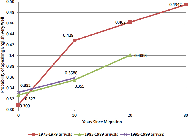
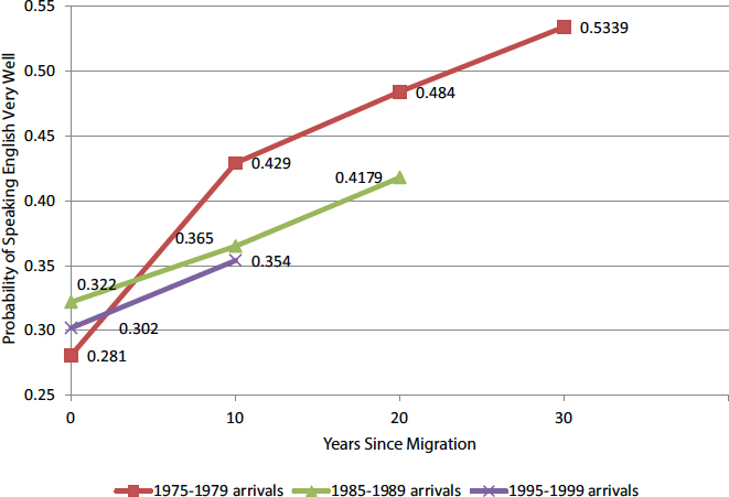
Following Borjas (2014b), Figures 3-6 and 3-7 show the assimilation profile for English-language proficiency of male and female wage-earning immigrants by arrival cohort. The age-adjusted probability of “speaking English very well” is calculated from a linear probability model estimated separately for datasets from the Decennial Census Public Use Microdata Series for 1970-2000 and the ACS Public Use Microdata Series for 2010-
NOTE: Regression coefficients reported in Table 3-28 (see Section 3.6).
2012, restricting the sample to immigrants originating in countries outside the British sphere of influence.14 The dependent variable is a dummy that is set to unity if the immigrant speaks only English or speaks English very well and is set to zero otherwise. The regressors include the worker’s age (introduced as a cubic polynomial). This regression analysis gives the following results:15
___________________
14 The intent here was to limit the sample to immigrants who had the chance to learn English over time, after arriving in the United States. The countries in the British sphere of influence are where English is widely spoken, which implies that immigrants from those source countries would be fluent in English at the time of entry into the United States. These countries are Antigua-Barbuda, Australia, Bahamas, Barbados, Belize-British Honduras, Bermuda, Canada, Dominican Republic, Grenada, Guyana/British Guiana, Ireland, Jamaica, Liberia, New Zealand, Northern Ireland, South Africa, St. Kitts-Nevis, St. Vincent, Trinidad and Tobago, and the United Kingdom.
15 For detailed results, see Tables 3-20 through 3-23 in the Technical Annex, Section 3.6.
- Male immigrants who arrived between 1975 and 1979 experienced a 12 percentage point increase in their fraction with English proficiency by 1990 and a 19 percentage point increase by 2012.
- The age-language proficiency profile for this arrival cohort is steeper than that of the 1985-1989 and 1995-1999 arrival cohorts.
- In the case of female immigrants, all arrival cohorts have a steeper age-language proficiency profile than male immigrants, although the general result holds that immigrants who arrived during the late 1980s and 1990s are slower in accumulating language skills than those who arrived in the late 1970s.
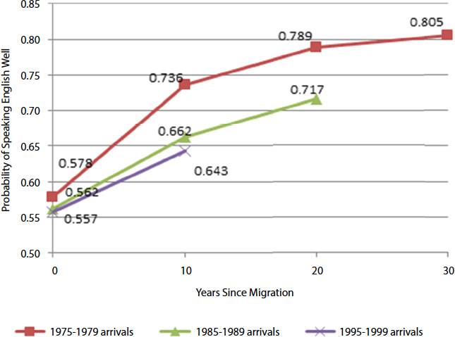
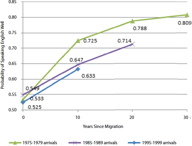
Figures 3-8 and 3-9 repeat the age-adjusted probability calculations but for a lower threshold of language proficiency: the probability of speaking English well (or better). These trends generally corroborate the finding discussed above that earlier cohorts of immigrants experienced more rapid language assimilation than recent cohorts. The relative slowdown of language assimilation may again be partly explained by high rates of immigra-
NOTE: Regression coefficients reported in Table 3-29 (see Section 3.6).
NOTE: Regression coefficients reported in Table 3-30 (see Section 3.6).
tion from Mexico during the 1990s. Lazear (2007) found that Mexicans start below immigrants from other countries in terms of English-language fluency and never catch up; in general, non-Hispanics were more fluent than Hispanics at all times after arrival in the United States. One possible explanation, articulated by Borjas (2014b, p. 35), is “immigrants who enter the country and find a large welcoming ethnic enclave have much less incentive to engage in these types of investments since they will find a large market for their pre-existing skills.”
Immigration policy also plays a role in patterns of wage convergence. Specifically, immigrants who enter the United States on work visas have different assimilation profiles than those on nonwork visas. Borjas and Friedberg (2009) examined the uptick in relative entry wages of immigrants who arrived between 1995 and 2000 and conjectured that expansion of the H1-B visa program was partly responsible. Chen (2011) found that work-visa holders with science and engineering degrees earned abroad experienced a higher rate of wage growth than nonwork-visa holders with
NOTE: Regression coefficients reported in Table 3-31 (see Section 3.6).
these degrees, but they did not reach economic parity with work-visa holders who had science and engineering degrees earned from U.S. institutions. The wage disadvantage was greater for nonwork-visa holders because they tended to concentrate in fields other than science and engineering, where there is less standardized, technical knowledge that is invariant and transferable across national boundaries. Chen also found that immigrant workers who possessed work visas upon first entry to the United States did not suffer from an earnings penalty, providing support for the notion that assimilation in these fields can be achieved without host-country-specific human capital. Chen attributed this finding to the universalism of science and engineering training and degrees (Chen, 2011). Orrenius and Zavodny (2014) investigated earnings of immigrants under Temporary Protected Status, a status typically granted if dangerous conditions are present in the immigrants’ home country due to war or a natural disaster. Using ACS data from 2005-2006, the authors compared labor market outcomes of men
and women immigrants from El Salvador, Mexico, and Guatemala. Their results suggested that being given legal status, even on a temporary basis, leads to better employment prospects for women and higher earnings for men relative to other immigrants with similar skills who were not granted Temporary Protected Status.
Evidence also exists indicating that place of education and source country characteristics influence labor market outcomes of U.S. immigrants. Zeng and Xie (2004) used data from the 1990 Decennial Census and the 1993 National Survey of College Graduates to compare earnings among native-born whites, native-born Asian-Americans, Asian immigrants educated in the United States, and Asian immigrants who completed education in their home country. Earnings differences between native-born groups and U.S.-educated Asian immigrants were small to negligible; however, Asian immigrants educated abroad earned 16 percent less than their counterparts who received U.S. degrees. Blau et al. (2011) investigated the impact of source country characteristics on the participation of married immigrant women in the U.S. labor force. They found that women immigrants from countries with high female labor force participation rates not only worked a greater number of annual hours than female immigrants from countries with low female labor force participation rates, they closed the gap with native-born women in 6 to 10 years. Borjas (2016a) revisited cohort effects and found that, in addition to average educational attainment at time of entry, gross domestic product (GDP) of source country affected economic assimilation of an immigrant cohort in its first 10 years. One explanation advanced by Borjas for the positive correlation between GDP of source country and economic assimilation is that skills of immigrants from high-income industrialized economies are more easily transferable to U.S. labor markets.
3.4 POVERTY AND WELFARE UTILIZATION
Comparative information about income status and welfare program use by different populations is essential to understanding the balance of fiscal benefits and the burdens that immigrants and their families bring to U.S. society.16 Examining trends related to native and immigrant poverty rates and program use over time also provides a perspective on assimilation different from but related to the trends associated with wages and employment. Because welfare programs comprise significant shares of federal, state, and local budgets, usage patterns by immigrants that differ from usage patterns of the native-born would imply that immigrants impose different fiscal burdens on these welfare programs.
___________________
16 The terms “safety net” and “welfare” are used interchangeably in this section.
By design, low-income households are more likely to access public benefits programs than are high-income households. As shown in Table 3-14 and Figure 3-10, immigrants experience higher poverty rates compared to the native-born; although, as the table indicates, this is not the case for
| In Poverty | In or Near Poverty | |||
|---|---|---|---|---|
| Immigrants | Immigrants and Their U.S.-born Children | Immigrants | Immigrants and Their U.S.-born Children | |
| Country of Birth | ||||
| Mexico | 30.1 | 34.8 | 62.9 | 67.8 |
| Honduras | 32.7 | 34.0 | 66.4 | 66.3 |
| Guatemala | 28.5 | 31.4 | 63.2 | 66.9 |
| Dominican Republic | 21.2 | 25.7 | 49.0 | 54.8 |
| Haiti | 23.7 | 25.2 | 49.5 | 49.5 |
| Cuba | 22.9 | 24.3 | 48.7 | 49.4 |
| Ecuador | 19.2 | 22.6 | 43.0 | 46.7 |
| El Salvador | 20.3 | 22.0 | 53.2 | 56.7 |
| Laos | 13.8 | 18.0 | 32.7 | 44.0 |
| Vietnam | 17.4 | 17.6 | 37.6 | 38.3 |
| Colombia | 14.9 | 16.0 | 31.0 | 33.6 |
| Jamaica | 12.2 | 16.0 | 33.5 | 37.1 |
| Iran | 16.2 | 15.2 | 32.7 | 32.8 |
| USSR/Russia | 12.5 | 12.9 | 12.8 | 30.7 |
| China | 14.0 | 13.6 | 33.4 | 30.8 |
| Peru | 10.1 | 13.6 | 32.4 | 36.4 |
| Pakistan | 11.0 | 11.9 | 30.6 | 32.9 |
| Korea | 9.7 | 11.1 | 23.8 | 24.8 |
| Japan | 12.1 | 10.1 | 26.2 | 25.0 |
| Canada | 9.1 | 8.0 | 19.4 | 18.1 |
| Poland | 7.2 | 7.5 | 32.1 | 30.5 |
| United Kingdom | 5.6 | 7.2 | 16.9 | 21.4 |
| Germany | 6.7 | 6.8 | 23.7 | 22.4 |
| India | 6.7 | 6.2 | 15.4 | 15.5 |
| Philippines | 6.3 | 5.5 | 19.4 | 20.1 |
| Region of Birth | ||||
| Middle East | 27.6 | 28.2 | 45.1 | 47.9 |
| In Poverty | In or Near Poverty | |||
|---|---|---|---|---|
| Immigrants | Immigrants and Their U.S.-born Children | Immigrants | Immigrants and Their U.S.-born Children | |
| Central America (excludes Mexico) | 25.2 | 26.8 | 56.8 | 59.1 |
| Sub-Saharan Africa | 22.9 | 24.6 | 42.9 | 46.2 |
| Caribbean | 19.4 | 22.0 | 43.4 | 46.2 |
| South America | 14.5 | 16.0 | 34.6 | 37.1 |
| East Asia | 12.4 | 12.8 | 30.0 | 30.6 |
| Europe | 9.5 | 10.1 | 27.6 | 27.8 |
| South Asia | 8.9 | 8.9 | 20.2 | 21.1 |
| All Immigrants | 19.9 | 23.0 | 43.6 | 47.6 |
| All Natives | 13.5 | 31.1 | ||
| Children of Immigrants (<18) | 32.1 | 59.2 | ||
| Children of Natives (<18) | 19.2 | 39.3 | ||
NOTE: The poverty and near-poverty percentages shown for “all natives” exclude U.S.-born children under age 18 of foreign-born fathers. “Immigrants and Their U.S.-born Children” includes U.S.-born children under age 18 of foreign-born fathers. “Near poverty” is defined as less than 200 percent of the federal poverty threshold.
SOURCE: Data from Camarota (2011, Table 10), based on the March 2011 Current Population Survey public use file.
immigrants from a subset of source countries (those toward the bottom of the list). In 2011, 19.9 percent of immigrants and 32.1 percent of children of immigrants17 (under 18) lived in poverty, compared to 13.5 percent of native-born persons and 19.2 percent of children of native-born. Suro et al. (2011) found that, for the period 2000 to 2009, immigrants living in suburbs experienced higher rates of poverty relative to the native-born living in suburbs; but their contribution to the growth of poor populations living in these areas (“the suburbanization of poverty”) was lower relative to that of the native-born.
___________________
17 Immigrants are defined here as the foreign-born as identified by the nativity variable in the CPS; the category thus includes naturalized citizens, lawful permanent residents, nonimmigrant visa holders, refugees, asylees, and unauthorized immigrants.
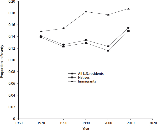
SOURCE: Reproduced from Card and Raphael (2013, Fig. 1.1, p. 5).
The primary reasons that immigrants experience higher levels of poverty than the native-born are that (as shown earlier in Tables 3-4, 3-5, 3-10, and 3-11) they are relatively less likely to be employed and they earn lower wages on average. And, as the analysis on fraction of time worked and wage assimilation in Section 3.3 shows, it takes some time for newly arrived immigrants to move up the job ladder and for the poor among them to lift themselves and their children out of poverty.
Another reason for the higher immigrant poverty rates stems from the shift in source countries away from Europe toward poorer countries in Asia and Latin America. Table 3-14, which shows the percentage of immigrants and their children in poverty and near poverty, reveals the wide variation in poverty experienced by immigrants from different countries. Poverty rates are higher for groups that form a larger proportion of the total immigrant population relative to those that comprise a smaller proportion (Table 2-1).
For example, 34.8 percent of Mexican immigrants and their U.S.-born children live in poverty, which is more than five times the corresponding statistic for immigrants and their U.S.-born children from countries such as India and the Philippines.
Additionally, there has been a change in the sectoral structure of the economy which affects the economic opportunities of low-skilled workers, including a large share of newly arriving immigrants. The United States has shifted from an industrial-based economy to a service-based economy that predominantly generates jobs with limited opportunities for economic mobility (Chen, 2011). The modern structure of the U.S. economy, with many jobs in the service sectors and high-skilled occupations but a shrinking number in between—in combination with less than full transferability of education and experience acquired abroad—has made it difficult for low-skilled immigrants to work their way out of poverty.
Comparatively high levels of poverty among immigrant groups relative to the native-born translates into greater participation in safety net programs. Although safety net programs are aimed at low-income families, children, and the elderly, not all immigrants have access due to restrictions imposed by law. Unauthorized immigrants and individuals on nonimmigrant visas are not eligible for the Supplemental Nutrition Assistance Program (SNAP), nonemergency Medicaid, Supplemental Security Income (SSI), and Temporary Assistance for Needy Families (TANF). The Personal Responsibility and Work Opportunity Reconciliation Act of 1996 (PRWORA) and the Illegal Immigration Reform and Immigrant Responsibility Act of 1996 (IIRIRA) introduced additional restrictions. The former made lawful permanent residents (LPRs) and certain other lawfully residing immigrants ineligible for federal means-tested public benefit programs (such as Medicaid) for the first 5 years after receiving the relevant status. The latter also included a provision intended to prevent states from extending in-state tuition benefits to unauthorized immigrants.18 LPRs who were previously eligible for assistance (before the enactment of these laws) became ineligible to receive assistance under the major federal benefits programs for a period of 5 years or longer. U.S.-born children of immigrants remained eligible for all programs, as they are citizens. Refugees and asylees also remained eligible for all programs.19 Subsequent amendments to the 1996 legislation restored benefits to legal immigrants for certain programs; for example, in 2002 SNAP eligibility was extended to qualified immigrant children without a waiting period.
___________________
18 There is a difference between being eligible for a welfare program and accepting benefits (taking up welfare). Participation rate is a combination of being eligible and taking up welfare.
19Capps et al. (2009) used CPS data to track welfare usage by refugee and asylees families between 1994 and 2004. There were sharp declines in TANF use, Medicaid and State Children’s Health Insurance Program coverage, and SNAP and SSI participation rates during that period.
One feature of PRWORA and IIRIRA is that states were allowed the option of providing fully state-funded safety net programs to legal immigrants not covered by federal programs. For example, several states or counties provide health coverage to children and/or pregnant women without a waiting period, regardless of their immigration status (Broder and Blazer, 2011). A report by the Pew Charitable Trusts (2014b) documented that 40 states and the District of Columbia either “supplement federal benefits programs with programs funded only by the states, or take the Unborn Child or CHIPRA [Children’s Health Insurance Program Reauthorization Act of 2009] options that expand the federal programs with state and federal matching funds . . . [while] only 10 states have neither provided their own programs for immigrants nor taken up one of the federal-state options to expand eligibility.”
While not carrying implications of the same magnitude as factors such as education and health, use of welfare programs certainly factors into the fiscal impact of immigration. Table 3-15, updating Camarota (2011), reports welfare usage by state for immigrant households with children and households led by native-born persons with children. Overall, these data show that the immigrant households use several programs, most notably food assistance and Medicaid, at higher rates than do households led by the native-born. The states with the highest usage rates for immigrant-headed households are Louisiana (77.8%), South Dakota (73.8%), New Mexico (72.5%) and Kansas (70.6%), while for native-headed households the highest-usage states are Arkansas (59.4%), Mississippi (55.2%), New Mexico (53.3%) and Louisiana (53.0%). The gap between immigrant and native-born welfare use is largest in Colorado, Minnesota, South Dakota, and Wisconsin. In these four states, immigrant households with children have a usage rate for any welfare that is an average 33 percentage points higher than the usage rate for native-born counterparts.
This higher use of welfare programs by immigrants is attributable to their lower average incomes and larger families. Bitler and Hoynes (2013) used 1995-2010 CPS data on TANF, food stamps (SNAP), Medicaid, State Children’s Health Insurance Program (SCHIP), SSI, school lunch, Low-Income Home Energy Assistance Program, and housing benefits to compare household-level participation in welfare programs between immigrant and native households with incomes less than 200 percent of the federal poverty level.20 The authors found that, among these lower-income households with children, those led by immigrants participated in some safety net programs at lower rates than did native-led households. This was evident for the 1995-2010 period for cash welfare, food stamps, and SSI. The authors
___________________
20 For the Bitler and Hoynes (2013) study, immigrant or native-born status was determined by the nativity of the household head.
went on to report that “children who are themselves immigrants are less likely to participate in Medicaid/SCHIP across the entire time period as well, and native children of immigrant parents about as likely as children of native parents to participate” (Bitler and Hoynes, 2013, p. 16). The main exception, they noted, was in the school lunch program, where low-income immigrant households with children consistently participated at higher rates than did native-born households. Figure 3-11 summarizes results from Bitler and Hoynes (2013). Graph (a), showing any safety net participation, is higher for low-income immigrant households than for corresponding native-born households primarily because of immigrant families’ higher participation in the school lunch program.21
Borjas (2011) also examined poverty and program participation among immigrant children22 using 1994-2009 CPS data on cash assistance, SNAP benefits, and Medicaid received by households. The children in that study were divided into four groups: (a) U.S.-born children who have one immigrant parent (mixed parentage), (b) U.S.-born children who have two immigrant parents, (c) foreign-born children who have two immigrant parents, and (d) U.S.-born children with U.S.-born parents. The analysis revealed that, even though poverty rates23 decreased for children (whether U.S.-born or foreign-born) with two immigrant parents between 1996 and 2000, they have increased since 2007. As shown in Figure 3-12, they have also gone up for children of the native-born but not as quickly. Also, among the four groups of children, the poverty rate was highest for foreign-born children with two immigrant parents. Children of mixed parentage had a group poverty rate not significantly different from children of two native-born parents. A similar conclusion can be drawn from the Borjas (2011) analysis of program participation rates (see Figure 3-13). U.S.-born children with two immigrant parents have the highest program participation rates among the four groups. This is not a surprising outcome, as their parents are likely to have the lowest income and, since they are U.S. born, the children are eligible for various safety net programs.
___________________
21Chapter 8 examines means-tested benefits by first, second, and third-plus generation immigrants (see Figure 8-15). The analysis there, based on 2011-2013 March CPS data, reveals that, between ages 20 and 60, the third-plus generation receives more means-tested antipoverty program benefits than either the first or second generations. Among the underlying factors are that recent arrivals do not qualify for many of these programs initially, and the second generation has a slightly more favorable socioeconomic status than does the third-plus generation. For a description of underreporting of means-tested transfer programs in the CPS and the Survey of Income and Program Participation, see Wheaton (2007).
22Borjas (2011) defined immigrant children as those who are foreign born and migrate to the United States with their foreign-born parents and those who are U.S. born to one or two immigrant (foreign-born) parents.
23 The poverty rate is defined as the fraction of children in a particular group that is being raised in households where family income is below the poverty threshold.
| State | Any Welfare | Cash Assistance | ||
|---|---|---|---|---|
| Immigrant | Native | Immigrant | Native | |
| Alabama | 52.4 | 49.5 | 1.1 | 8.4 |
| Alaska | 49.2 | 38.5 | 5.4 | 4.6 |
| Arizona | 55.1 | 42.6 | 3.0 | 5.5 |
| Arkansas | 69.1 | 59.4 | 5.0 | 7.3 |
| California | 61.5 | 40.7 | 9.5 | 9.4 |
| Colorado | 62.0 | 31.4 | 3.5 | 4.6 |
| Connecticut | 45.8 | 32.4 | 3.8 | 4.1 |
| Delaware | 58.2 | 41.0 | 3.2 | 7.2 |
| District of Columbia | 63.4 | 50.5 | 3.6 | 21.1 |
| Florida | 57.3 | 42.8 | 3.4 | 4.7 |
| Georgia | 51.2 | 45.0 | 2.0 | 4.5 |
| Hawaii | 55.3 | 45.9 | 8.1 | 6.9 |
| Idaho | 64.4 | 41.0 | 1.6 | 3.7 |
| Illinois | 59.1 | 41.6 | 2.0 | 4.3 |
| Indiana | 57.6 | 44.4 | 1.0 | 5.4 |
| Iowa | 50.5 | 40.3 | 3.2 | 4.9 |
| Kansas | 70.6 | 40.8 | 2.9 | 5.5 |
| Kentucky | 60.1 | 49.6 | 2.7 | 9.1 |
| Louisiana | 77.8 | 53.0 | 5.1 | 6.9 |
| Maine | 50.8 | 45.7 | 5.6 | 9.3 |
| Maryland | 42.3 | 31.7 | 1.1 | 4.0 |
| Massachusetts | 48.6 | 34.7 | 8.1 | 9.1 |
| Michigan | 48.3 | 43.6 | 6.1 | 7.4 |
| Minnesota | 66.9 | 29.1 | 11.4 | 4.4 |
| Mississippi | 45.9 | 55.2 | 4.5 | 7.9 |
| Missouri | 54.7 | 40.1 | 1.1 | 7.3 |
| Montana | 29.4 | 45.5 | 0.0 | 6.4 |
| Nebraska | 66.0 | 33.0 | 5.0 | 4.2 |
| Nevada | 49.5 | 36.6 | 4.4 | 4.1 |
| New Hampshire | 30.3 | 26.5 | 2.8 | 3.6 |
| New Jersey | 46.4 | 28.9 | 4.1 | 5.4 |
| New Mexico | 72.5 | 53.3 | 8.8 | 6.6 |
| New York | 64.2 | 42.2 | 7.8 | 7.4 |
| North Carolina | 58.6 | 44.3 | 2.3 | 5.8 |
| Food Assistance | Housing | Medicaid | |||
|---|---|---|---|---|---|
| Immigrant | Native | Immigrant | Native | Immigrant | Native |
| 42.8 | 38.2 | 5.1 | 4.3 | 39.5 | 41.6 |
| 31.8 | 24.1 | 5.2 | 4.7 | 41.7 | 30.0 |
| 48.9 | 30.4 | 0.9 | 2.9 | 39.4 | 34.5 |
| 57.5 | 45.4 | 5.3 | 4.9 | 59.9 | 51.3 |
| 48.0 | 28.2 | 4.2 | 4.9 | 49.2 | 32.0 |
| 49.3 | 20.8 | 9.1 | 3.8 | 46.4 | 25.1 |
| 28.3 | 20.6 | 3.4 | 6.6 | 39.6 | 27.6 |
| 37.9 | 28.7 | 5.6 | 8.1 | 45.0 | 34.8 |
| 46.7 | 40.0 | 8.6 | 24.0 | 53.7 | 46.0 |
| 43.5 | 30.4 | 1.8 | 3.3 | 43.5 | 33.6 |
| 40.3 | 34.4 | 0.5 | 4.7 | 37.2 | 34.0 |
| 38.5 | 29.2 | 13.8 | 8.7 | 41.4 | 39.3 |
| 56.7 | 33.1 | 2.1 | 4.2 | 42.7 | 32.1 |
| 43.0 | 29.7 | 0.8 | 5.1 | 49.7 | 35.2 |
| 46.6 | 33.1 | 4.0 | 8.9 | 37.8 | 37.4 |
| 37.8 | 28.9 | 0.8 | 1.8 | 37.9 | 34.0 |
| 61.7 | 31.9 | 6.6 | 6.6 | 51.3 | 30.7 |
| 51.1 | 39.4 | 7.1 | 5.1 | 50.1 | 40.8 |
| 55.8 | 39.5 | 3.0 | 6.5 | 59.5 | 46.5 |
| 37.5 | 33.3 | 28.0 | 5.3 | 47.0 | 40.9 |
| 32.7 | 20.1 | 1.9 | 4.3 | 31.2 | 25.2 |
| 32.4 | 22.5 | 13.0 | 7.5 | 44.5 | 31.2 |
| 34.9 | 33.1 | 2.3 | 4.4 | 43.4 | 36.6 |
| 54.3 | 19.3 | 12.2 | 3.5 | 54.2 | 23.5 |
| 38.1 | 46.1 | 0.0 | 7.9 | 26.4 | 43.5 |
| 37.6 | 29.5 | 6.5 | 5.2 | 47.8 | 30.9 |
| 23.6 | 32.9 | 7.5 | 7.6 | 19.5 | 35.9 |
| 58.0 | 24.9 | 13.6 | 4.3 | 38.9 | 23.5 |
| 42.1 | 28.5 | 2.9 | 5.6 | 25.3 | 22.8 |
| 18.7 | 13.6 | 2.0 | 2.3 | 21.5 | 23.3 |
| 30.3 | 18.1 | 4.3 | 5.1 | 37.5 | 24.1 |
| 57.4 | 35.9 | 9.3 | 5.6 | 62.3 | 44.6 |
| 44.0 | 27.9 | 8.5 | 9.2 | 55.3 | 34.5 |
| 50.0 | 35.0 | 4.0 | 5.0 | 49.4 | 37.1 |
| State | Any Welfare | Cash Assistance | ||
|---|---|---|---|---|
| Immigrant | Native | Immigrant | Native | |
| North Dakota | 30.7 | 34.9 | 0.0 | 3.9 |
| Ohio | 66.5 | 44.2 | 4.6 | 7.8 |
| Oklahoma | 57.4 | 52.3 | 2.2 | 6.7 |
| Oregon | 51.9 | 44.3 | 4.9 | 6.7 |
| Pennsylvania | 46.2 | 42.2 | 3.8 | 6.5 |
| Rhode Island | 64.1 | 38.7 | 4.6 | 8.6 |
| South Carolina | 56.1 | 46.5 | 1.2 | 6.0 |
| South Dakota | 73.8 | 41.8 | 7.4 | 5.9 |
| Tennessee | 58.1 | 46.8 | 4.9 | 7.8 |
| Texas | 63.7 | 44.2 | 2.8 | 5.3 |
| Utah | 57.0 | 32.1 | 2.2 | 3.5 |
| Vermont | 57.5 | 52.5 | 8.9 | 7.7 |
| Virginia | 34.3 | 28.5 | 2.2 | 4.7 |
| Washington | 63.5 | 41.7 | 7.1 | 4.3 |
| West Virginia | 27.1 | 49.9 | 20.3 | 8.5 |
| Wisconsin | 67.9 | 36.9 | 5.7 | 4.8 |
| Wyoming | 56.9 | 35.8 | 0.0 | 4.3 |
| TOTAL | 58.2 | 41.8 | 5.5 | 6.3 |
NOTES: Current Population Survey data for 2011, 2012, and 2013, restricted to households with at least one child under the age of 18. Immigrant households are based on the head of household’s immigrant status (where the head of household is considered immigrant if they are not a citizen or are a naturalized citizen). “Any welfare” encompasses cash assistance (SSI and
| Food Assistance | Housing | Medicaid | |||
|---|---|---|---|---|---|
| Immigrant | Native | Immigrant | Native | Immigrant | Native |
| 21.5 | 23.9 | 2.3 | 6.6 | 21.5 | 25.2 |
| 55.9 | 34.9 | 3.3 | 5.5 | 55.8 | 35.1 |
| 43.8 | 39.3 | 0.0 | 4.8 | 48.8 | 41.4 |
| 44.4 | 33.6 | 3.1 | 3.9 | 39.6 | 36.2 |
| 33.2 | 28.3 | 2.0 | 5.4 | 34.6 | 36.2 |
| 51.3 | 27.7 | 10.8 | 9.6 | 50.2 | 33.4 |
| 44.0 | 37.9 | 2.0 | 5.0 | 35.7 | 35.2 |
| 56.6 | 33.0 | 15.8 | 8.4 | 61.1 | 33.9 |
| 43.2 | 35.5 | 7.8 | 4.1 | 45.1 | 39.4 |
| 55.2 | 34.6 | 1.8 | 5.8 | 45.6 | 33.9 |
| 47.7 | 24.6 | 5.4 | 3.4 | 33.9 | 20.1 |
| 33.1 | 31.0 | 21.2 | 4.6 | 47.7 | 47.9 |
| 24.1 | 21.1 | 1.4 | 5.3 | 27.0 | 21.8 |
| 52.8 | 30.4 | 8.7 | 3.8 | 55.2 | 33.2 |
| 10.3 | 37.6 | 6.4 | 4.3 | 27.1 | 40.5 |
| 59.2 | 25.8 | 1.7 | 3.2 | 50.4 | 32.4 |
| 46.3 | 24.4 | 4.0 | 5.1 | 48.5 | 29.0 |
| 45.3 | 30.6 | 4.2 | 5.3 | 45.7 | 33.8 |
TANF), food assistance (WIC, free or reduced-price school lunch, and food stamps), housing assistance (public housing and rent subsidies), and Medicaid.
SSI = Supplemenal Security Income; TANF = Temporary Assistance for Needy Families; WIC = Special Supplemental Nutrition Program for Women, Infants, and Children.
SOURCE: Panel’s calculations from Current Population Survey 2011-2013 data.
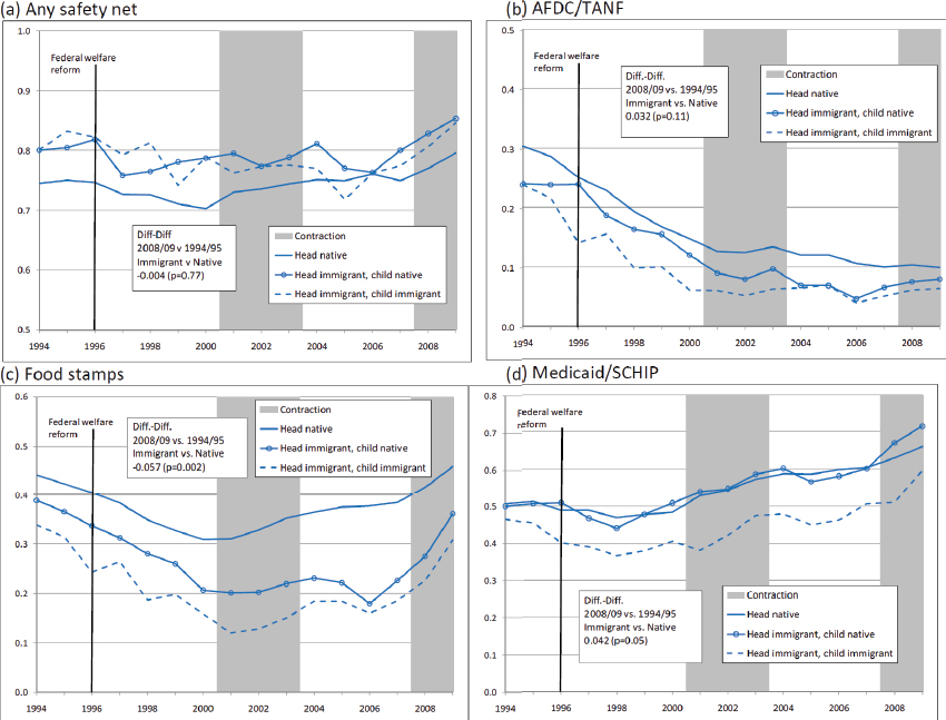
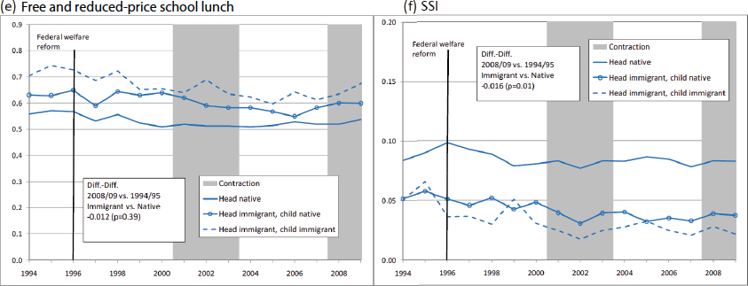
NOTE: Calculations are from the 1995–2010 Annual Social and Economic Supplement data of the Current Population Survey. Sample included children under 18 with household income below 200% of poverty level. Program participation was measured at the household level. Any safety net program participation means someone in the household (1) participated in public assistance, food stamps (SNAP), Medicaid, free or reduced-price school lunch, Supplemental Security Income, or public housing or (2) received a rental subsidy from the government or energy assistance. Figures are weighted. Shaded areas refer to annual periods of labor market contraction. See source text for explanation of the weighting applied to the data shown in the graphs and further details of the analytical methodology.
SOURCE: Bitler and Hoynes (2013, Figs. 11.3-11.8, pp. 333-338).
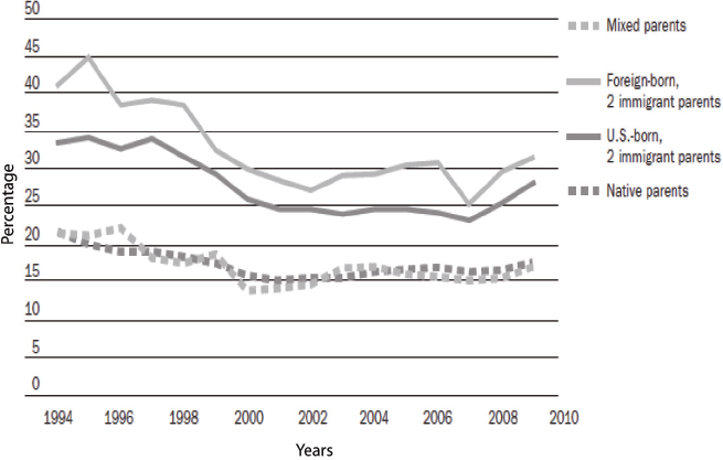
SOURCE: Borjas (2011, Fig. 2, p. 251). The author’s calculations are based on data from the 1994-2009 March Current Population Survey administrations. The poverty rate is the percentage of households with incomes below the poverty threshold.
3.5 CONCLUSIONS
This chapter examined how trends in the skills of immigrants—particularly their education and experience—compare to those of the native-born population. The relative skill compositions of the two populations are an important determinant of the economic consequences of immigration, along with the magnitude of immigrant inflows and the share of immigrants likely to increase the productivity of other workers. The chapter also described how employment rates and wages of immigrants have compared with those of the native-born population.
Although the native-born population increased during the period of analysis, the total foreign-born population size expanded much more, resulting in an increase in the share of the foreign-born in the total population. And, aside from children younger than age 15, the foreign-born population changed from being a relatively old population in 1970 to being a relatively young population, with a peak concentration of persons ages 25-34 in 2012.
Education levels of immigrant arrival cohorts have been steadily rising over time, a trend observed for both men and women. That said, as explored
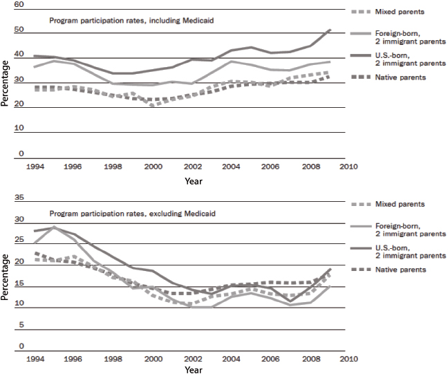
SOURCE: Borjas (2011, Fig. 3, p. 253). Author’s calculations are based on data from 1994-2009 March CPS administrations. The program participation rate gives the fraction of children living in households that received cash assistance, Supplemental Nutrition Assistance Program (SNAP) benefits, or Medicaid (in the top panel), or cash assistance and SNAP benefits (in the bottom panel).
in Chapter 5, the impact of immigration on the wages and employment of the native-born population is most directly related to relative education levels. While there is a consistent gap in educational attainment between the native-born and the foreign-born, with the former enjoying the advantage, there is a trend toward convergence between the two groups in the average education levels for adults ages 25-34—a category in which about half of recent immigrants in each year fall. In 1970, the mean education for persons ages 25-34 was 12.1 (years of education) for the native-born and 11.6 for a recently arrived immigrant; by 1980, the gap had expanded from 0.5 years to 1.8 years, with mean years of education of 13.1 and 11.9, respectively. By 2012, the gap narrowed substantially to 0.3 years,
with a mean of 13.7 years of education for the native-born and 13.4 for the recently arrived foreign-born. Across all age groups combined, however, no such convergence in educational attainment is observed.
Over this period, the educational attainment of the foreign-born population has consistently been more varied than that of the native-born population. This contrast is particularly pronounced for young adults. In 1970, 41 percent of the foreign-born ages 30-34 had not completed high school, compared to 30 percent of the native-born. In the same age group, also in 1970, the foreign-born population had 11 percent with more than college education, compared to the native-born at 6 percent. In 2012, again restricting to individuals ages 30-34, 29 percent of the foreign-born had less than high school education, compared to 8 percent of the native-born. At the high end, 13 percent of the foreign-born, versus 11 percent of the native-born, had more than college education.
Occupational sorting has also changed in recent decades. While foreign-born workers are overrepresented in high-level professional groups that require the most education (such as scientists, engineers, and architects), they are underrepresented among other professionals, managers, and sales personnel. It is interesting to note that growth in the share of foreign-born workers in these occupations has been slower than growth in the share of foreign-born workers in the general labor force, resulting in a relative decline of foreign-born workers in these relatively high-status occupations.
Employment outcomes provide one indication of the pace and extent to which immigrants integrate into the United States. Shortly after arrival in the United States, immigrant men—especially recent cohorts—experience a disadvantage relative to native-born men in terms of the probability of being employed. However, for cohorts of immigrants arriving since the 1970s, after this initial period of adjustment in which their probability of employment is lower, they became slightly more likely to be employed than their native-born peers. The higher employment rate among immigrant men is mainly represented in the population with education of a high school degree or less, and the difference in employment ratios between immigrant and native-born men is due mainly to differences in labor force participation and not to unemployment. Immigrant women display lower employment rates than immigrant men and, typically, lower rates than native-born women. However, their probability of being employed relative to native-born women also rises appreciably after 10 years of U.S. residence, as immigrant women are exposed to U.S. labor market conditions and social norms and as some experience changes in their visa status, which improves their chances of finding employment.
On the wage front, as their time spent in the U.S. workforce extends, immigrants tend to catch up with their native-born peers. Male immigrants who arrived between 1965 and 1969 experienced rapid growth in their
relative wages, which allowed them to close the gap with native-born peers. This indication of economic integration has shown signs of slowing in more recent decades. The relative wage profile has flattened somewhat across recent arrival cohorts, indicating a slowing rate of wage convergence. This overall conclusion holds after controlling for immigrants’ educational attainment, although the relative wage picture for immigrants is considerably more favorable when education is controlled for. Compared to male immigrants, female immigrants start off with a less dramatic wage disadvantage, but they experience slower growth in their wages relevant to native-born peers than do male immigrants.
Regarding poverty and program participation, a key change since The New Americans report (National Research Council, 1997) was welfare reform that restricted program access to some immigrants. One implication of that legislation for immigrants has been a lowering of participation rates in means-tested programs, which impacts their capacity to navigate through challenging economic times. The Great Recession of 2007-2009 and subsequent slow recovery, combined with the changing sectoral composition of the economy, has created difficult economic conditions for immigrants and the native-born alike, especially those at the low-skilled end of the labor spectrum.
3.6 TECHNICAL ANNEX OF TABULATIONS AND REGRESSION RESULTS
| Immigrants in 1970 (%) |
Immigrants in 1980 (%) |
Immigrants in 1990 (%) |
Immigrants in 2000 (%) |
Immigrants in 2012 (%) |
|
|---|---|---|---|---|---|
| Less than High School | 47 | 37 | 37 | 36 | 27 |
| High School Diploma / GED | 15 | 16 | 17 | 17 | 20 |
| Some College | 11 | 18 | 17 | 14 | 14 |
| Bachelor’s Degree | 9 | 12 | 15 | 17 | 21 |
| Graduate Education | 19 | 18 | 15 | 16 | 18 |
| N (all attainment levels) | 426,700 | 787,420 | 1,258,276 | 2,022,420 | 1,853,249 |
SOURCE: Analyses of 1970-2000 Decennial Census data and 2010-2012 American Community Survey data, accessed through the Integrated Public Use Microdata Series.
| Immigrants in 1970 (%) |
Immigrants in 1980 (%) |
Immigrants in 1990 (%) |
Immigrants in 2000 (%) |
Immigrants in 2012 (%) |
|
|---|---|---|---|---|---|
| Less than High School | 54 | 44 | 40 | 35 | 25 |
| High School Diploma / GED | 23 | 22 | 20 | 19 | 20 |
| Some College | 10 | 16 | 17 | 16 | 16 |
| Bachelor’s Degree | 7 | 10 | 15 | 18 | 24 |
| Graduate Education | 6 | 9 | 8 | 12 | 15 |
| N (all attainment levels) | 506,333 | 812,320 | 1,267,141 | 1,972,390 | 2,057,872 |
SOURCE: Analyses of 1970-2000 Decennial Census data and 2010-2012 American Community Survey data, accessed through the Integrated Public Use Microdata Series.
| Share of Male Workers in Occupation Who are Foreign Born | ||||||
|---|---|---|---|---|---|---|
| 1970 | 1980 | 1990 | 2000 | 2012 | Share of All Male Workers with a Bachelor’s or Higher Degree in 2012 | |
| Across All Occupations Occupation | 4.8 | 6.2 | 8.6 | 11.8 | 18.7 | 34.6 |
|
Lawyers and judges |
2.5 | 2.2 | 2.8 | 3.6 | 5.2 | 99.1 |
|
Physicians, dentists, and related |
11.5 | 14.2 | 14.5 | 18.3 | 22.6 | 98.4 |
|
Mathematicians |
6.7 | 8.6 | 9.4 | 16.5 | 21.4 | 96.5 |
|
Postsecondary teachers |
11.0 | 11.4 | 15.9 | 17.8 | 26.2 | 95.6 |
|
Preschool and elementary teachers |
3.0 | 2.9 | 4.0 | 5.5 | 6.4 | 95.5 |
|
Physical scientists |
10.0 | 10.5 | 12.1 | 21.8 | 28.7 | 95.0 |
|
Life scientists |
9.5 | 7.2 | 10.4 | 19.5 | 28.9 | 93.5 |
|
Architects |
7.5 | 9.4 | 11.2 | 11.5 | 18.3 | 89.1 |
|
Social and recreation workers |
4.0 | 4.3 | 5.6 | 8.2 | 10.4 | 88.5 |
|
Librarians, archivists, and curators |
6.5 | 8.2 | 7.5 | 8.0 | 8.4 | 86.6 |
|
Accountants and financial analysts |
4.1 | 5.9 | 7.8 | 9.4 | 12.7 | 81.0 |
|
Engineers |
6.8 | 9.4 | 11.7 | 15.2 | 19.5 | 79.8 |
|
Secondary, vocational, and adult ed. Teachers |
2.8 | 3.5 | 5.3 | 5.8 | 8.2 | 75.7 |
|
Religious workers |
5.3 | 4.9 | 5.8 | 8.1 | 11.9 | 75.2 |
|
Administrators and public officers |
2.2 | 3.0 | 4.1 | 6.3 | 7.8 | 72.9 |
|
Nurses, dieticians, therapists |
4.5 | 6.1 | 8.0 | 12.3 | 18.7 | 68.0 |
| Share of Male Workers in Occupation Who are Foreign Born | ||||||
|---|---|---|---|---|---|---|
| 1970 | 1980 | 1990 | 2000 | 2012 | Share of All Male Workers with a Bachelor’s or Higher Degree in 2012 | |
|
Social scientists |
6.6 | 7.3 | 7.2 | 10.4 | 13.9 | 67.2 |
|
Computer specialists |
4.4 | 6.6 | 10.0 | 17.2 | 23.5 | 66.5 |
|
Writers, artists, and media workers |
7.0 | 7.2 | 8.0 | 9.8 | 12.4 | 60.9 |
|
Managers and proprietors |
4.6 | 5.8 | 7.6 | 9.7 | 13.7 | 54.3 |
|
Sales workers, retail |
5.2 | 5.3 | 8.8 | 11.4 | 17.1 | 50.2 |
|
Secretaries |
5.5 | 7.1 | 8.3 | 9.8 | 14.5 | 37.8 |
|
All other technicians |
4.7 | 5.5 | 7.8 | 8.0 | 10.8 | 35.1 |
|
Bookkeepers |
6.0 | 9.1 | 12.3 | 14.0 | 16.6 | 33.5 |
|
Health service workers |
4.1 | 8.5 | 11.9 | 16.7 | 24.0 | 32.6 |
|
Sales workers |
3.4 | 4.5 | 6.6 | 7.7 | 10.9 | 32.3 |
|
Clerical workers |
3.7 | 5.1 | 7.6 | 10.4 | 14.9 | 26.9 |
|
Protective service workers |
1.7 | 2.6 | 3.3 | 4.9 | 7.1 | 25.7 |
|
Health technicians |
8.6 | 11.8 | 12.5 | 12.4 | 16.3 | 19.0 |
|
Personal service workers and barbers |
10.5 | 12.7 | 15.7 | 19.0 | 28.9 | 17.6 |
|
Farmers and farm laborers, incl. forestry and fishing |
2.7 | 3.9 | 7.5 | 14.5 | 26.9 | 13.4 |
|
Cleaning service and food service workers |
10.5 | 14.2 | 20.2 | 25.2 | 35.5 | 9.1 |
|
Craftsmen |
5.1 | 6.7 | 9.2 | 13.0 | 20.4 | 8.9 |
|
Electricians |
3.6 | 3.8 | 5.3 | 7.0 | 12.0 | 7.9 |
|
Construction workers |
4.6 | 5.6 | 8.4 | 12.0 | 25.5 | 7.2 |
|
Operators, except textile, metalworking, and transportation |
5.6 | 7.1 | 9.3 | 12.4 | 19.6 | 7.2 |
|
Mechanical workers |
4.0 | 5.1 | 6.6 | 9.0 | 14.5 | 7.1 |
|
Textile machine operators |
13.3 | 18.1 | 23.6 | 32.0 | 49.0 | 6.8 |
|
Carpenters |
7.3 | 7.5 | 8.6 | 12.6 | 28.1 | 6.3 |
|
Metalworking and transportation operators |
3.3 | 4.6 | 7.0 | 10.6 | 20.1 | 5.9 |
|
Laborers, except farm |
5.0 | 7.8 | 11.8 | 18.6 | 32.8 | 5.7 |
NOTE: “Workers” is defined as those who are employed and work at least 50 weeks a year in a nonmilitary occupation. Occupational categories are the Tier 1 categories in Section 3.7, Technical Annex on Occupational Categories.
SOURCE: Analyses of 1970-2000 Decennial Census data and 2010-2012 American Community Survey data, accessed through the Integrated Public Use Microdata Series.
| Share of Female Workers in Occupation Who Are Foreign Born | Share of All Female Workers with a Bachelor’s or Higher Degree in 2012 | |||||
|---|---|---|---|---|---|---|
| 1970 | 1980 | 1990 | 2000 | 2012 | ||
| Across all occupations Occupations | 5.4 | 6.7 | 8.0 | 10.2 | 15.8 | 36.5 |
|
Lawyers and judges |
5.0 | 3.3 | 4.2 | 5.5 | 8.2 | 97.5 |
|
Physical scientists |
18.0 | 16.2 | 16.6 | 27.9 | 30.8 | 97.2 |
|
Life scientists |
9.4 | 13.4 | 12.7 | 24.1 | 32.2 | 96.8 |
|
Architects |
21.1 | 14.0 | 15.6 | 18.0 | 21.4 | 94.9 |
|
Postsecondary teachers |
8.8 | 8.2 | 10.8 | 11.8 | 18.9 | 94.3 |
|
Physicians, dentists, and related |
29.4 | 28.4 | 20.3 | 22.5 | 23.1 | 92.6 |
|
Social and recreation workers |
4.1 | 3.8 | 4.6 | 6.5 | 8.6 | 88.1 |
|
Mathematicians |
6.6 | 7.4 | 11.8 | 15.4 | 23.3 | 87.7 |
|
Preschool and elementary teachers |
2.1 | 3.1 | 4.1 | 5.4 | 7.2 | 87.6 |
|
Librarians, archivists, and curators |
6.1 | 5.7 | 6.2 | 6.6 | 6.7 | 86.9 |
|
Engineers |
6.5 | 9.1 | 10.6 | 18.1 | 25.3 | 85.4 |
|
Secondary, vocational, and adult ed teachers |
3.6 | 4.0 | 4.7 | 5.7 | 8.5 | 81.2 |
|
Administrators and public officers |
2.7 | 3.2 | 4.1 | 5.4 | 7.8 | 72.0 |
|
Social scientists |
5.3 | 6.8 | 6.2 | 9.2 | 10.9 | 70.6 |
|
Writers, artists, and media workers |
7.0 | 6.4 | 6.4 | 8.2 | 11.1 | 68.2 |
|
Religious workers |
5.2 | 4.7 | 5.4 | 6.2 | 8.3 | 66.1 |
|
Computer specialists |
4.7 | 7.0 | 9.9 | 14.5 | 21.8 | 64.7 |
|
Nurses, dieticians, therapists |
5.5 | 7.3 | 8.0 | 10.1 | 13.2 | 60.5 |
|
Accountants and financial analysts |
4.8 | 6.8 | 7.7 | 10.3 | 14.7 | 59.9 |
|
Managers and proprietors |
5.0 | 5.3 | 5.9 | 7.7 | 11.0 | 52.3 |
|
Sales workers, retail |
5.3 | 6.3 | 8.8 | 10.8 | 16.8 | 41.4 |
|
All other technicians |
4.7 | 6.6 | 7.4 | 8.6 | 12.5 | 38.6 |
|
Health service workers |
5.1 | 6.7 | 9.4 | 12.7 | 19.1 | 27.2 |
|
Protective service workers |
3.5 | 3.9 | 3.7 | 5.3 | 7.1 | 27.2 |
|
Sales workers |
4.6 | 6.0 | 6.8 | 8.4 | 12.0 | 22.8 |
|
Clerical workers |
4.1 | 5.2 | 6.1 | 7.3 | 10.9 | 20.1 |
|
Secretaries |
4.1 | 4.2 | 4.8 | 5.5 | 7.5 | 18.6 |
|
Construction workers |
5.2 | 5.7 | 7.2 | 9.3 | 16.0 | 18.1 |
|
Mechanical workers |
3.7 | 4.7 | 5.9 | 7.9 | 13.3 | 17.7 |
|
Farmers and farm laborers, including forestry and fishing |
3.8 | 4.6 | 8.4 | 17.2 | 32.6 | 16.4 |
|
Bookkeepers |
4.3 | 4.6 | 5.9 | 7.0 | 9.7 | 15.3 |
|
Electricians |
3.1 | 5.9 | 7.9 | 10.5 | 11.7 | 13.8 |
|
Personal service workers and barbers |
6.5 | 9.9 | 13.8 | 14.6 | 26.5 | 12.0 |
|
Craftsmen |
5.9 | 9.7 | 13.1 | 17.7 | 27.0 | 11.0 |
|
Carpenters |
6.9 | 7.2 | 8.7 | 11.5 | 20.3 | 10.8 |
|
Health technicians |
8.8 | 7.8 | 6.9 | 8.0 | 10.8 | 7.9 |
|
Laborers, except farm |
5.0 | 8.9 | 9.7 | 16.1 | 28.7 | 7.5 |
|
Cleaning service and food service workers |
6.3 | 10.0 | 13.6 | 20.4 | 35.6 | 7.4 |
|
Operators, except textile, metalworking, and transportation |
6.7 | 10.3 | 13.4 | 17.7 | 30.7 | 7.1 |
|
Metalworking and transportation operators |
5.6 | 5.9 | 5.7 | 6.3 | 11.7 | 6.2 |
|
Textile machine operators |
11.0 | 16.3 | 20.4 | 30.5 | 50.5 | 6.1 |
NOTE: “Workers” is defined as those who are employed and work at least 50 weeks a year in a nonmilitary occupation. Occupational categories are the Tier 1 categories in Section 3.7, Technical Annex on Occupational Categories.
SOURCE: Analyses of 1970-2000 Decennial Census data and 2010-2012 American Community Survey data, accessed through the Integrated Public Use Microdata Series.
| Variables | Census | ACS | ||||||||
|---|---|---|---|---|---|---|---|---|---|---|
| 1970 | 1980 | 1990 | 2000 | 2012 | ||||||
| Coeff | Robust SE | Coeff | Robust SE | Coeff | Robust SE | Coeff | Robust SE | Coeff | Robust SE | |
| 2010-2012 | –0.158 | 0.001 | ||||||||
| 2005-2009 | 0.011 | 0.001 | ||||||||
| 2000-2004 | 0.056 | 0.001 | ||||||||
| 1995-1999 | –0.160 | 0.001 | 0.057 | 0.001 | ||||||
| 1990-1994 | –0.047 | 0.001 | 0.044 | 0.000 | ||||||
| 1985-1989 | –0.185 | 0.001 | –0.033 | 0.001 | 0.042 | 0.000 | ||||
| 1980-1984 | –0.048 | 0.001 | –0.032 | 0.000 | 0.042 | 0.000 | ||||
| 1975-1979 | –0.183 | 0.001 | –0.019 | 0.001 | –0.019 | 0.000 | 0.046 | 0.000 | ||
| 1970-1974 | –0.025 | 0.001 | –0.016 | 0.000 | –0.011 | 0.000 | 0.034 | 0.001 | ||
| 1965-1969 | –0.107 | 0.001 | –0.010 | 0.000 | 0.005 | 0.000 | 0.012 | 0.001 | 0.022 | 0.001 |
| 1960-1964 | 0.000 | 0.001 | 0.005 | 0.000 | 0.021 | 0.000 | 0.018 | 0.002 | 0.033 | 0.001 |
| 1950-1959 | 0.014 | 0.000 | 0.019 | 0.000 | 0.034 | 0.001 | 0.024 | 0.002 | 0.038 | 0.002 |
SOURCE: Analyses of 1970-2000 Decennial Census data and 2010-2012 American Community Survey data, accessed through the Integrated Public Use Microdata Series.
| Variables | Census | ACS | ||||||||
|---|---|---|---|---|---|---|---|---|---|---|
| 1970 | 1980 | 1990 | 2000 | 2012 | ||||||
| Coeff | Robust SE | Coeff | Robust SE | Coeff | Robust SE | Coeff | Robust SE | Coeff | Robust SE | |
| 2010-2012 | –0.158 | 0.001 | ||||||||
| 2005-2009 | 0.040 | 0.008 | ||||||||
| 2000-2004 | 0.098 | 0.012 | ||||||||
| 1995-1999 | –0.135 | 0.003 | 0.098 | 0.012 | ||||||
| 1990-1994 | –0.011 | 0.006 | 0.086 | 0.012 | ||||||
| 1985-1989 | –0.156 | 0.003 | 0.013 | 0.008 | 0.087 | 0.013 | ||||
| 1980-1984 | –0.008 | 0.005 | 0.012 | 0.008 | 0.085 | 0.013 | ||||
| 1975-1979 | –0.164 | 0.001 | 0.023 | 0.006 | 0.019 | 0.007 | 0.083 | 0.011 | ||
| 1970-1974 | 0.004 | 0.002 | 0.026 | 0.006 | 0.027 | 0.008 | 0.077 | 0.014 | ||
| 1965-1969 | –0.101 | 0.000 | 0.013 | 0.002 | 0.030 | 0.004 | 0.037 | 0.006 | 0.050 | 0.010 |
| 1960-1964 | 0.008 | 0.000 | 0.017 | 0.001 | 0.035 | 0.002 | 0.030 | 0.004 | 0.039 | 0.003 |
| 1950-1959 | 0.023 | 0.000 | 0.026 | 0.001 | 0.043 | 0.003 | 0.030 | 0.004 | 0.032 | 0.002 |
SOURCE: Analyses of 1970-2000 Decennial Census data and 2010-2012 American Community Survey data, accessed through the Integrated Public Use Microdata Series.
| Variables | Census | ACS | ||||||||
|---|---|---|---|---|---|---|---|---|---|---|
| 1970 | 1980 | 1990 | 2000 | 2012 | ||||||
| Coeff | Robust SE | Coeff | Robust SE | Coeff | Robust SE | Coeff | Robust SE | Coeff | Robust SE | |
| 2010-2012 | –0.369 | 0.002 | ||||||||
| 2005-2009 | –0.208 | 0.002 | ||||||||
| 2000-2004 | –0.131 | 0.001 | ||||||||
| 1995-1999 | –0.295 | 0.002 | –0.097 | 0.001 | ||||||
| 1990-1994 | –0.173 | 0.001 | –0.063 | 0.000 | ||||||
| 1985-1989 | –0.255 | 0.001 | –0.131 | 0.001 | –0.031 | 0.000 | ||||
| 1980-1984 | –0.111 | 0.001 | –0.086 | 0.000 | –0.010 | 0.001 | ||||
| 1975-1979 | –0.163 | 0.001 | –0.074 | 0.000 | –0.063 | 0.000 | –0.016 | 0.002 | ||
| 1970-1974 | –0.033 | 0.001 | –0.053 | 0.000 | –0.049 | 0.001 | –0.022 | 0.002 | ||
| 1965-1969 | –0.014 | 0.000 | –0.001 | 0.000 | –0.023 | 0.000 | –0.030 | 0.001 | –0.005 | 0.002 |
| 1960-1964 | 0.004 | 0.000 | –0.009 | 0.000 | –0.014 | 0.000 | –0.025 | 0.002 | –0.002 | 0.002 |
| 1950-1959 | –0.011 | 0.000 | –0.011 | 0.000 | –0.016 | 0.001 | –0.016 | 0.002 | 0.015 | 0.002 |
SOURCE: Analyses of 1970-2000 Decennial Census data and 2010-2012 American Community Survey data, accessed through the Integrated Public Use Microdata Series.
| Variables | Census | ACS | ||||||||
|---|---|---|---|---|---|---|---|---|---|---|
| 1970 | 1980 | 1990 | 2000 | 2012 | ||||||
| Coeff | Robust SE | Coeff | Robust SE | Coeff | Robust SE | Coeff | Robust SE | Coeff | Robust SE | |
| 2010-2012 | –0.353 | 0.001 | ||||||||
| 2005-2009 | –0.170 | 0.003 | ||||||||
| 2000-2004 | –0.075 | 0.006 | ||||||||
| 1995-1999 | –0.256 | 0.002 | –0.041 | 0.007 | ||||||
| 1990-1994 | –0.117 | 0.004 | –0.005 | 0.008 | ||||||
| 1985-1989 | –0.200 | 0.005 | –0.070 | 0.005 | 0.021 | 0.008 | ||||
| 1980-1984 | –0.042 | 0.007 | –0.030 | 0.006 | 0.038 | 0.008 | ||||
| 1975-1979 | –0.118 | 0.002 | –0.006 | 0.007 | –0.015 | 0.005 | 0.027 | 0.008 | ||
| 1970-1974 | 0.017 | 0.003 | 0.007 | 0.007 | –0.005 | 0.006 | 0.023 | 0.009 | ||
| 1965-1969 | 0.014 | 0.000 | 0.039 | 0.003 | 0.017 | 0.005 | –0.001 | 0.005 | 0.025 | 0.008 |
| 1960-1964 | 0.027 | 0.000 | 0.017 | 0.002 | 0.011 | 0.004 | –0.006 | 0.005 | 0.009 | 0.005 |
| 1950-1959 | 0.009 | 0.001 | 0.007 | 0.002 | 0.003 | 0.004 | –0.004 | 0.005 | 0.014 | 0.005 |
SOURCE: Analyses of 1970-2000 Decennial Census data and 2010-2012 American Community Survey data, accessed through the Integrated Public Use Microdata Series.
| Variables | Census | ACS | ||||||||
|---|---|---|---|---|---|---|---|---|---|---|
| 1970 | 1980 | 1990 | 2000 | 2012 | ||||||
| Coeff | Robust SE | Coeff | Robust SE | Coeff | Robust SE | Coeff | Robust SE | Coeff | Robust SE | |
| 2010-2012 | –.1971 | .0041 | ||||||||
| 2005-2009 | –.3106 | .0044 | ||||||||
| 2000-2004 | –.3388 | .0027 | ||||||||
| 1995-1999 | –0.273 | 0.004 | –.2692 | .0010 | ||||||
| 1990-1994 | –0.269 | 0.003 | –.2662 | .0035 | ||||||
| 1985-1989 | –0.331 | 0.001 | –0.269 | 0.002 | –.2521 | .0056 | ||||
| 1980-1984 | –0.285 | 0.001 | –0.236 | 0.002 | –.2094 | .0060 | ||||
| 1975-1979 | –0.314 | 0.001 | –0.185 | 0.001 | –0.176 | 0.005 | –.1357 | .0047 | ||
| 1970-1974 | –0.223 | 0.001 | –0.124 | 0.002 | –0.128 | 0.006 | –.0054 | .0045 | ||
| 1965-1969 | –0.235 | 0.001 | –0.122 | 0.001 | –0.02 | 0.003 | –0.014 | 0.005 | .1760 | .0103 |
| 1960-1964 | –0.058 | 0.001 | –0.041 | 0.001 | 0.046 | 0.004 | 0.074 | 0.004 | 1.1337 | .0181 |
| 1950-1959 | 0.037 | 0.001 | 0.032 | 0.001 | 0.1 | 0.003 | 0.147 | 0.01 | ||
SOURCE: Analyses of 1970-2000 Decennial Census data and 2010-2012 American Community Survey data, accessed through the Integrated Public Use Microdata Series.
| Variables | Census | ACS | ||||||||
|---|---|---|---|---|---|---|---|---|---|---|
| 1970 | 1980 | 1990 | 2000 | 2012 | ||||||
| Coeff | Robust SE | Coeff | Robust SE | Coeff | Robust SE | Coeff | Robust SE | Coeff | Robust SE | |
| 2010-2012 | –.064 | .017 | ||||||||
| 2005-2009 | –.136 | .028 | ||||||||
| 2000-2004 | –.130 | .029 | ||||||||
| 1995-1999 | –.149 | .021 | –.074 | .023 | ||||||
| 1990-1994 | –.099 | .025 | –.075 | .018 | ||||||
| 1985-1989 | –.176 | .015 | –.056 | .025 | –.026 | .019 | ||||
| 1980-1984 | –.098 | .017 | –.039 | .020 | –.003 | .014 | ||||
| 1975-1979 | –.211 | .0041 | .011 | .016 | .039 | .019 | .069 | .012 | ||
| 1970-1974 | –.087 | .0047 | .075 | .014 | .088 | .017 | .120 | .004 | ||
| 1965-1969 | –0.172 | .0025 | –0.030 | .002 | .099 | .006 | .133 | .008 | .111 | .017 |
| 1960-1964 | 0.003 | .0023 | 0.015 | .0004 | .133 | .002 | .133 | .004 | .987 | .025 |
| 1950-1959 | 0.01 | .0017 | 0.077 | .0018 | .186 | .001 | .096 | .018 | ||
SOURCE: Analyses of 1970-2000 Decennial Census data and 2010-2012 American Community Survey data, accessed through the Integrated Public Use Microdata Series.
| Variables | Census | ACS | ||||||||
|---|---|---|---|---|---|---|---|---|---|---|
| 1970 | 1980 | 1990 | 2000 | 2012 | ||||||
| Coeff | Robust SE | Coeff | Robust SE | Coeff | Robust SE | Coeff | Robust SE | Coeff | Robust SE | |
| 2010-2012 | –.2782 | .0033 | ||||||||
| 2005-2009 | –.3143 | .0031 | ||||||||
| 2000-2004 | –.2989 | .0021 | ||||||||
| 1995-1999 | –0.216 | 0.002 | –.2395 | .0010 | ||||||
| 1990-1994 | –0.165 | 0.002 | –.2027 | .0027 | ||||||
| 1985-1989 | –0.184 | 0.001 | –0.138 | 0.001 | –.1684 | .0048 | ||||
| 1980-1984 | –0.093 | 0.000 | –0.100 | 0.002 | –.0975 | .0054 | ||||
| 1975-1979 | –0.082 | 0.000 | –0.002 | 0.000 | –0.053 | 0.004 | –.0312 | .0040 | ||
| 1970-1974 | 0.026 | 0.001 | 0.042 | 0.001 | –0.026 | 0.005 | .0615 | .0041 | ||
| 1965-1969 | –0.021 | 0.001 | 0.068 | 0.001 | 0.083 | 0.002 | 0.023 | 0.004 | .1329 | .0104 |
| 1960-1964 | 0.037 | 0.001 | 0.036 | 0.000 | 0.061 | 0.002 | 0.043 | 0.003 | .1706 | .0189 |
| 1950-1959 | 0.051 | 0.000 | 0.025 | 0.001 | 0.013 | 0.002 | 0.173 | 0.008 | ||
SOURCE: Analyses of 1970-2000 Decennial Census data and 2010-2012 American Community Survey data, accessed through the Integrated Public Use Microdata Series.
| Variables | Census | ACS | ||||||||
|---|---|---|---|---|---|---|---|---|---|---|
| 1970 | 1980 | 1990 | 2000 | 2012 | ||||||
| Coeff | Robust SE | Coeff | Robust SE | Coeff | Robust SE | Coeff | Robust SE | Coeff | Robust SE | |
| 2010-2012 | –.230 | .009 | ||||||||
| 2005-2009 | –.154 | .019 | ||||||||
| 2000-2004 | –.114 | .020 | ||||||||
| 1995-1999 | –.075 | .019 | –.056 | .018 | ||||||
| 1990-1994 | .002 | .021 | –.010 | .016 | ||||||
| 1985-1989 | –.009 | .020 | .060 | .023 | .027 | .014 | ||||
| 1980-1984 | .120 | .024 | .0091 | .021 | .078 | .010 | ||||
| 1975-1979 | .038 | .008 | .201 | .023 | .135 | .019 | .142 | .010 | ||
| 1970-1974 | .162 | .009 | .224 | .020 | .131 | .014 | .160 | .004 | ||
| 1965-1969 | .111 | .007 | .173 | .008 | .202 | .012 | .133 | .008 | .073 | .010 |
| 1960-1964 | .142 | .006 | .102 | .005 | .143 | .008 | .111 | .002 | –.017 | .019 |
| 1950-1959 | .144 | .005 | .080 | .004 | .101 | .008 | .123 | .013 | ||
SOURCE: Analyses of 1970-2000 Decennial Census data and 2010-2012 American Community Survey data, accessed through the Integrated Public Use Microdata Series.
| Variables | Census | ACS | ||||||
|---|---|---|---|---|---|---|---|---|
| 1980 | 1990 | 2000 | 2012 | |||||
| Coeff | Robust SE | Coeff | Robust SE | Coeff | Robust SE | Coeff | Robust SE | |
| 2010-2012 Arrivals | .3676 | .0202 | ||||||
| 2005-2009 Arrivals | .3098 | .0211 | ||||||
| 2000-2004 Arrivals | .3144 | .0163 | ||||||
| 1995-1999 Arrivals | 0.332 | 0.015 | .3588 | .0098 | ||||
| 1990-1994 Arrivals | 0.346 | 0.013 | .3756 | .0048 | ||||
| 1985-1989 Arrivals | 0.327 | 0.005 | 0.355 | 0.007 | .4008 | .0062 | ||
| 1980-1984 Arrivals | 0.369 | 0.005 | 0.408 | 0.005 | .4489 | .0110 | ||
| 1975-1979 Arrivals | 0.309 | 0.005 | 0.428 | 0.003 | 0.462 | 0.008 | .4947 | .0164 |
| 1970-1974 Arrivals | 0.364 | 0.004 | 0.480 | 0.003 | 0.517 | 0.013 | .5999 | .0279 |
| 1965-1969 Arrivals | 0.432 | 0.004 | 0.561 | 0.005 | 0.598 | 0.017 | .7173 | .0439 |
| 1960-1964 Arrivals | 0.532 | 0.008 | 0.654 | 0.007 | 0.706 | 0.025 | .8257 | .0625 |
| 1950-1959 Arrivals | 0.672 | 0.017 | 0.754 | 0.013 | 0.821 | 0.037 | ||
SOURCE: Analyses of 1980-2000 Decennial Census data and 2010-2012 American Community Survey data, accessed through the Integrated Public Use Microdata Series.
| Variables | Census | ACS | ||||||
|---|---|---|---|---|---|---|---|---|
| 1980 | 1990 | 2000 | 2012 | |||||
| Coeff | Robust SE | Coeff | Robust SE | Coeff | Robust SE | Coeff | Robust SE | |
| 2010-2012 Arrivals | .3300 | .0154 | ||||||
| 2005-2009 Arrivals | .2907 | .0143 | ||||||
| 2000-2004 Arrivals | .3080 | .0101 | ||||||
| 1995-1999 Arrivals | 0.302 | 0.013 | .3540 | .0060 | ||||
| 1990-1994 Arrivals | 0.333 | 0.011 | .3733 | .0038 | ||||
| 1985-1989 Arrivals | 0.322 | 0.008 | 0.365 | 0.005 | .4179 | .0061 | ||
| 1980-1984 Arrivals | 0.360 | 0.007 | 0.422 | 0.005 | .4895 | .0108 | ||
| 1975-1979 Arrivals | 0.281 | 0.009 | 0.429 | 0.004 | 0.484 | 0.008 | .5339 | .0151 |
| 1970-1974 Arrivals | 0.341 | 0.007 | 0.508 | 0.004 | 0.572 | 0.013 | .6084 | .0219 |
| 1965-1969 Arrivals | 0.424 | 0.006 | 0.596 | 0.006 | 0.660 | 0.016 | .7335 | .0315 |
| 1960-1964 Arrivals | 0.543 | 0.009 | 0.714 | 0.010 | 0.767 | 0.021 | .7948 | .0435 |
| 1950-1959 Arrivals | 0.716 | 0.019 | 0.829 | 0.020 | 0.902 | 0.028 | ||
SOURCE: Analyses of 1980-2000 Decennial Census data and 2010-2012 American Community Survey data, accessed through the Integrated Public Use Microdata Series.
| Variables | Census | ACS | ||||||
|---|---|---|---|---|---|---|---|---|
| 1980 | 1990 | 2000 | 2012 | |||||
| Coeff | Robust SE | Coeff | Robust SE | Coeff | Robust SE | Coeff | Robust SE | |
| 2010-2012 Arrivals | 0.604 | 0.018 | ||||||
| 2005-2009 Arrivals | 0.533 | 0.019 | ||||||
| 2000-2004 Arrivals | 0.572 | 0.015 | ||||||
| 1995-1999 Arrivals | 0.557 | 0.01 | 0.643 | 0.009 | ||||
| 1990-1994 Arrivals | 0.632 | 0.009 | 0.69 | 0.003 | ||||
| 1985-1989 Arrivals | 0.562 | 0.006 | 0.662 | 0.005 | 0.717 | 0.005 | ||
| 1980-1984 Arrivals | 0.663 | 0.005 | 0.725 | 0.003 | 0.777 | 0.009 | ||
| 1975-1979 Arrivals | 0.578 | 0.009 | 0.736 | 0.003 | 0.789 | 0.005 | 0.805 | 0.011 |
| 1970-1974 Arrivals | 0.666 | 0.008 | 0.779 | 0.002 | 0.827 | 0.008 | 0.847 | 0.018 |
| 1965-1969 Arrivals | 0.747 | 0.003 | 0.866 | 0.006 | 0.889 | 0.012 | 0.857 | 0.028 |
| 1960-1964 Arrivals | 0.854 | 0.006 | 0.944 | 0.008 | 0.937 | 0.016 | 0.816 | 0.041 |
| 1950-1959 Arrivals | 0.993 | 0.013 | 0.986 | 0.01 | 0.954 | 0.023 | ||
SOURCE: Analyses of 1980-2000 Decennial Census data and 2010-2012 American Community Survey data, accessed through the Integrated Public Use Microdata Series.
| Variables | Census | ACS | ||||||
|---|---|---|---|---|---|---|---|---|
| 1980 | 1990 | 2000 | 2012 | |||||
| Coeff | Robust SE | Coeff | Robust SE | Coeff | Robust SE | Coeff | Robust SE | |
| 2010-2012 Arrivals | 0.573 | 0.02 | ||||||
| 2005-2009 Arrivals | 0.529 | 0.019 | ||||||
| 2000-2004 Arrivals | 0.572 | 0.013 | ||||||
| 1995-1999 Arrivals | 0.525 | 0.015 | 0.633 | 0.006 | ||||
| 1990-1994 Arrivals | 0.607 | 0.012 | 0.664 | 0.004 | ||||
| 1985-1989 Arrivals | 0.549 | 0.01 | 0.647 | 0.006 | 0.714 | 0.008 | ||
| 1980-1984 Arrivals | 0.633 | 0.008 | 0.717 | 0.004 | 0.773 | 0.012 | ||
| 1975-1979 Arrivals | 0.533 | 0.011 | 0.725 | 0.004 | 0.788 | 0.007 | 0.809 | 0.016 |
| 1970-1974 Arrivals | 0.613 | 0.009 | 0.794 | 0.002 | 0.859 | 0.011 | 0.851 | 0.02 |
| 1965-1969 Arrivals | 0.707 | 0.006 | 0.879 | 0.004 | 0.919 | 0.014 | 0.874 | 0.027 |
| 1960-1964 Arrivals | 0.845 | 0.007 | 0.972 | 0.008 | 0.962 | 0.017 | 0.796 | 0.035 |
| 1950-1959 Arrivals | 1 | 0.014 | 1 | 0.01 | 0.984 | 0.021 | ||
SOURCE: Analyses of 1980-2000 Decennial Census data and 2010-2012 American Community Survey data, accessed through the Integrated Public Use Microdata Series.
3.7 TECHNICAL ANNEX ON OCCUPATIONAL CATEGORIES
The occupational analysis in Chapter 3 tracks changes in concentration of native-born and foreign-born individuals in different occupational categories. Because the occupational structure of a labor market changes over time, an occupational coding system that takes into account such changes is required. Xie and Killewald (2012) and Xie et al. (2016) created such a coding system, which is useful for tracking occupational changes over time. This system, based on classification of 41 occupational categories—and reproduced below—was created to meet two conflicting objectives to the extent possible: (1) reduce the number of occupational categories, and (2) group detailed occupations only when socioeconomic status and work content are sufficiently similar across these occupations. With the second purpose in mind, the second-tier occupational categories are 8 major occupational categories that are generated by collapsing the 41 occupational categories. This two-tier occupational coding system is the basis for Tables 3-18 and 3-19.
First-Tier Occupational Categories
Lawyers and judges: Lawyers; Judges, magistrates, and other judicial workers
Physicians, dentists, and related practitioners: Chiropractors; Dentists; Optometrists; Physicians and surgeons; Podiatrists; Audiologists; Veterinarians; Health diagnosing and treating practitioners, all other
Mathematicians: Actuaries; Mathematicians; Statisticians; Miscellaneous mathematical science occupations; Professors and postsecondary instructors, mathematical (imputed in 2000 and 2007)
Postsecondary teachers: Postsecondary teachers
Preschool and elementary teachers: Preschool and kindergarten teachers; Elementary and middle school teachers
Physical scientists: Astronomers and physicists; Atmospheric and space scientists; Chemists and materials scientists; Environmental scientists and geoscientists; Physical scientists, all other; Professors and postsecondary instructors, physical sciences (imputed in 2000 and 2007)
Life scientists: Agriculture and food scientists; Biological scientists; Conservation scientists and foresters; Medical scientists; Professors and postsecondary instructors, life sciences (imputed in 2000 and 2007)
Architects: Architects, except naval
Social and recreation workers: Counselors; Social workers; Miscellaneous community and social service specialists; Recreation and fitness workers; Residential advisors
Librarians, archivists, and curators: Archivists, curators, and museum technicians; Librarians
Accountants and financial analysts: Financial managers; Cost estimators; Accountants and auditors; Budget analysts; Credit analysts; Financial analysts; Personal financial advisors; Insurance underwriters; Financial examiners; Loan counselors and officers; Tax examiners, collectors, and revenue agents; Tax preparers; Financial specialists, all other
Engineers: Aerospace engineers; Agricultural engineers; Biomedical engineers; Chemical engineers; Civil engineers; Computer hardware engineers; Electrical and electronics engineers; Environmental engineers; Industry engineers, including health and safety; Materials engineers; Mechanical engineers; Mining and geological engineers, including mining safety engineers; Nuclear engineers; Petroleum engineers; Engineers, all other; Sales engineers; Professors and postsecondary instructors, engineering (imputed in 2000 and 2007)
Secondary, vocational, and adult education teachers: Secondary school teachers; Special education teachers; Other teachers and instructors; Other education, training, and library workers
Religious workers: Clergy; Directors, religious activities and education; Religious workers, all other
Administrators and public officers: Legislators; Administrative services managers; Education administrators; Natural sciences managers; Postmasters and mail superintendents; Social and community service managers; Compliance officers, except agriculture, construction, health and safety, and transportation
Nurses, dietitians, therapists: Dietitians and nutritionists; Pharmacists; Physician assistants; Registered nurses; Occupational therapists; Physical therapists; Radiation therapists; Recreational therapists; Respiratory therapists; Speech-language therapists; Therapists, all other; Massage therapists
Social scientists: Economists; Market and survey researchers; Psychologists; Sociologists; Urban and regional planners; Miscellaneous social scientists and related workers
Computer specialists: Computer scientists and systems analysts; Computer programmers; Computer software engineers; Computer support specialists; Database administrators; Network and computer systems administrators; Network systems and data communications analysts; Operations research analysts; Computer
control programmers and operators; Professors and postsecondary instructors, computer science (imputed in 2000 and 2007)
Writers, artists and media workers: Artists and related workers; Designers; Actors; Producers and directors; Athletes, coaches, umpires, and related workers; Dancers and choreographers; Musicians, singers, and related workers; Entertainers and performers, sports and related workers, all other; Announcers; News analysts, reporters and correspondents; Public relations specialists; Editors; Technical writers; Writers and authors; Photographers
Managers and proprietors: Chief executives; General and operations managers; Advertising and promotions managers; Marketing and sales managers; Public relations managers; Computer and information systems managers; Human resources managers; Industrial production managers; Purchasing managers; Transportation, storage, and distribution managers; Farm, ranch, and other agricultural managers; Construction managers; Engineering managers; Food service managers; Funeral directors; Gaming managers; Lodging managers; Medical and health services managers; Property, real estate, and community association managers; Managers, all other; Purchasing agents and buyers, farm products; Wholesale and retail buyers, except farm products; Purchasing agents, except wholesale, retail and farm products; Human resources, training, and labor relations specialists; Management analysts; Other business operations specialists
Sales workers, retail: First-line supervisors/managers of retail sales workers; Cashiers; Counter and rental clerks; Parts salespersons; Retail salespersons; Door-to-door sales workers, news and street vendors, and related workers
Secretaries: Secretaries and administrative assistants
All other technicians: Appraisers and assessors of real estate; Surveyors, cartographers, and photogrammetrists; Marine engineers and naval architects; Drafters; Engineering technicians, except drafters; Surveying and mapping technicians; Agricultural and food science technicians; Biological technicians; Chemical technicians; Geological and petroleum technicians; Nuclear technicians; Other life, physical, and social science technicians; Paralegals and legal assistants; Miscellaneous legal support workers; Library technicians; Miscellaneous media and communication workers; Broadcast and sound engineering technicians and radio operators; Television, video, and motion picture camera operators and editors; Media and communication equipment workers, all other; Animal trainers; Aircraft pilots and flight engineers; Air traffic controllers and airfield operations specialists; Locomotive engineers and operators; Railroad
brake, signal, and switch operators; Railroad conductors and yardmasters; Subway, streetcar, and other rail transportation workers; Ship and boat captains and operators; Ship engineers; Bridge and lock tenders; Transportation inspectors
Bookkeepers: Bookkeeping, accounting, and auditing clerks
Health service workers: Licensed practical and licensed vocational nurses; Nursing, psychiatric, and home health aides; Occupational therapist assistants and aides; Physical therapist assistants and aides; Dental assistants; Medical assistant and other health care support occupations
Sales workers: Agents and business managers of artists, performers, and athletes; First-line supervisors/managers of nonretail sales workers; Advertising sales agents; Insurance sales agents; Securities, commodities, and financial service sales agents; Travel agents; Sales representatives, services, all other; Sales representatives, wholesale and manufacturing; Models, demonstrators, and product promoters; Real estate brokers and sales agents; Telemarketers; Sales and related workers, all other; Reservation and transportation ticket agents and travel clerks
Clerical workers: Claims adjusters, appraisers, examiners, and investigators; Logisticians; Meeting and convention planners; Teacher assistants; First-line supervisors/managers of gaming workers; Gaming service workers; First-line supervisors/managers of office and administrative support workers; Switchboard operators, including answering service; Telephone operators; Communications equipment operators, all other; Bill and account collectors; Billing and posting clerks and machine operators; Gaming cage workers; Payroll and timekeeping clerks; Procurement clerks; Tellers; Brokerage clerks; Correspondence clerks; Court, municipal, and license clerks; Credit authorizers, checkers, and clerks; Customer service representatives; Eligibility interviewers, government programs; File clerks; Hotel, motel, and resort desk clerks; Interviewers, except eligibility and loan; Library assistants, clerical; Loan interviewers and clerks; New accounts clerks; Order clerks; Human resources assistants, except payroll and timekeeping; Receptionists and information clerks; Information and record clerks, all other; Cargo and freight agents; Couriers and messengers; Dispatchers; Meter readers, utilities; Postal service clerks; Postal service mail carriers; Postal service mail sorters, processors, and processing machine operators; Production, planning, and expediting clerks; Shipping, receiving, and traffic clerks; Stock clerks and order fillers; Weighers, measurers, checkers, and samplers, recordkeeping; Computer operators; Data entry keyers; Word processors and typists; Desktop publishers; Insurance claims and
policy processing clerks; Mail clerks and mail machine operators, except postal service; Office clerks, general; Office machine operators, except computer; Proofreaders and copy markers; Statistical assistants; Office and administrative support workers, all other
Protective service workers: First-line supervisors/managers of correctional officers; First-line supervisors/managers of police and detectives; First-line supervisors/managers of fire fighting and prevention workers; Supervisors, protective service workers, all other; Firefighters; Fire inspectors; Bailiffs, correctional officers, and jailers; Detectives and criminal investigators; Parking enforcement workers; Police and sheriff’s patrol officers; Transit and railroad police; Animal control workers; Private detectives and investigators; Security guards and gaming surveillance officers; Crossing guards; Lifeguards and other protective service workers
Health technicians: Clinical laboratory technologists and technicians; Dental hygienists; Diagnostic related technologists and technicians; Emergency medical technicians and paramedics; Health diagnosing and treating practitioner support technicians; Medical records and health information technicians; Opticians, dispensing; Miscellaneous health technologists and technicians; Other health care practitioners and technical occupations; Medical, dental, and ophthalmic laboratory technicians
Personal service workers and barbers: First-line supervisors/managers of personal service workers; Ushers, lobby attendants, and ticket takers; Miscellaneous entertainment attendants and related workers; Funeral service workers; Barbers; Hairdressers, hairstylists, and cosmetologists; Miscellaneous personal appearance workers; Baggage porters, bellhops, and concierges; Tour and travel guides; Transportation attendants; Child care workers; Personal and home care aides; Personal care and service workers, all other; Parking lot attendants
Farmers and farm laborers, including forestry and fishing: Farmers and ranchers; Fish and game wardens; First-line supervisors/managers of farming, fishing, and forestry workers; Agricultural inspectors; Animal breeders; Graders and sorters, agricultural products; Miscellaneous agricultural workers; Fishers and related fishing workers; Hunters and trappers; Forest and conservation workers; Logging workers
Cleaning service and food service workers: Chefs and head cooks; First-line supervisors/managers of food preparation and serving workers; Cooks; Food preparation workers; Bartenders; Combined food preparation and serving workers, including fast food; Counter attendants, cafeteria, food concession, and coffee shop; Waiters
and waitresses; Food servers, nonrestaurant; Dining room and cafeteria attendants and bartender helpers; Dishwashers; Hosts and hostesses, restaurant, lounge, and coffee shop; Food preparation and serving related workers, all other; First-line supervisors/managers of housekeeping and janitorial workers; First-line supervisors/managers of landscaping, lawn service, and groundskeeping workers; Janitors and building cleaners; Maids and housekeeping cleaners; Pest control workers
Craftsmen: Boilermakers; Millwrights; First-line supervisors/managers of production and operating workers; Aircraft structure, surfaces, rigging, and systems assemblers; Electrical, electronics, and electromechanical assemblers; Structural metal fabricators and fitters; Bakers; Food batchmakers; Model makers and patternmakers, metal and plastic; Molders and molding machine setters, operators, and tenders, metal and plastic; Tool and die makers; Welding, soldering, and brazing workers; Lay-out workers, metal and plastic; Tool grinders, filers, and sharpeners; Metalworkers and plastic workers, all other; Bookbinders and bindery workers; Fabric and apparel patternmakers; Upholsterers; Furniture finishers; Jewelers and precious stone and metal workers; Photographic process workers and processing machine operators; Semiconductor processors; Etchers and engravers; Molders, shapers, and casters, except metal and plastic; Tire builders
Electricians: Electricians; Electrical power-line installers and repairers; Precision instrument and equipment repairers
Construction workers: First-line supervisors/managers of construction trades and extraction workers; Brickmasons, blockmasons, and stonemasons; Carpet, floor, and tile installers and finishers; Cement masons, concrete finishers, and terrazzo workers; Paving, surfacing, and tamping equipment operators; Pile-driver operators; Drywall installers, ceiling tile installers, and tapers; Glaziers; Insulation workers; Painters, construction and maintenance; Paperhangers; Pipelayers, plumbers, pipefitters, and steamfitters; Plasterers and stucco masons; Reinforcing iron and rebar workers; Roofers; Sheet metal workers; Structural iron and steel workers; Construction and building inspectors; Fence erectors; Hazardous materials removal workers; Septic tank services and sewer pipe cleaners; Miscellaneous construction and related workers; Manufactured building and mobile home installers
Operators, except textile, metalworking and transportation: Motion picture projectionists; Operating engineers and other construction equipment operators; Derrick, rotary drill, and service unit operators, oil, gas, and mining; Earth drillers, except oil and gas;
Explosives workers, ordinance handling experts, and blasters; Mining machine operators; Roof bolters, mining; Other extraction workers; Miscellaneous assemblers and fabricators; Butchers and other meat, poultry, and fish processing workers; Food and tobacco roasting, baking, and drying machine operators and tenders; Food cooking machine operators and tenders; Job printers; Prepress technicians and workers; Printing machine operators; Extruding and forming machine setters, operators, and tenders, synthetic and glass fibers; Sawing machine setters, operators, and tenders, wood; Power plant operators, distributors, and dispatchers; Stationary engineers and boiler operators; Water and liquid waste treatment plant and system operators; Miscellaneous plant and system operators; Chemical processing machine setters, operators, and tenders; Crushing, grinding, polishing, mixing, and blending workers; Cutting workers; Furnace, kiln, oven, drier, and kettle operators and tenders; Inspectors, testers, sorters, samplers, and weighers; Packaging and filling machine operators and tenders; Painting workers; Cementing and gluing machine operators and tenders; Cooling and freezing equipment operators and tenders; Paper goods machine setters, operators, and tenders; Production workers, all others; Conveyor operators and tenders; Crane and tower operators; Dredge, excavating, and loading machine operators; Hoist and winch operators
Mechanical workers: Elevator installers and repairers; First-line supervisors/managers of mechanics, installers, and repairers; Computer, automated teller, and office machine repairers; Radio and telecommunications equipment installers and repairers; Avionics technicians; Electric motor, power tool, and related repairers; Electrical and electronics installers and repairers, transportation equipment; Electrical and electronics repairers, industrial and utility; Electronic equipment installers and repairers, motor vehicles; Electronic home entertainment equipment installers and repairers; Security and fire alarm systems installers; Aircraft mechanics and service technicians; Automotive body and related repairers; Automotive glass installers and repairers; Automotive service technicians and mechanics; Bus and truck mechanics and diesel engine specialists; Heavy vehicle and mobile equipment service technicians and mechanics; Small engine mechanics; Miscellaneous vehicle and mobile equipment mechanics, installers, and repairers; Control and valve installers and repairers; Heating, air conditioning, and refrigeration mechanics and installers; Home appliance repairers; Industrial and refractory machinery mechanics; Maintenance and repair workers, general; Maintenance workers, machinery;
Telecommunications line installers and repairers; Coin, vending, and amusement machine services and repairers; Locksmiths and safe repairers; Riggers; Signal and track switch repairers; Engine and other machine assemblers
Textile machine operators: Laundry and dry-cleaning workers; Pressers, textile, garment, and related materials; Sewing machine operators; Shoe and leather workers and repairers; Shoe machine operators and tenders; Tailors, dressmakers, and sewers; Textile bleaching and dyeing machine operators and tenders; Textile cutting machine setters, operators, and tenders; Textile knitting and weaving machine setters, operators, and tenders; Textile winding, twisting, and drawing out machine setters, operators, and tenders; Textile, apparel, and furnishings workers, all other
Carpenters: Carpenters; Cabinetmakers and bench carpenters; Model makers and patternmakers, wood; Woodworking machine setters, operators, and tenders, except sawing; Woodworkers, all other
Metalworking and transportation operators: Highway maintenance workers; Rail-track laying and maintenance equipment operators; Commercial drivers; Extruding and drawing machine setters, operators, and tenders, metal and plastic; Forging machine setters, operators, and tenders, metal and plastic; Rolling machine setters, operators, and tenders, metal and plastic; Cutting, punching, and press machine setters, operators, and tenders, metal and plastic; Drilling and boring machine tool setters, operators, and tenders, metal and plastic; Grinding, lapping, polishing, and buffing machine tool setters, operators, and tenders, metal and plastic; Lathe and turning machine tool setters, operators, and tenders, metal and plastic; Milling and planing machine setters, operators, and tenders, metal and plastic; Machinists; Metal furnace and kiln operators and tenders; Multiple machine tool setters, operators, and tenders, metal and plastic; Heat treating equipment setters, operators, and tenders, metal and plastic; Plating and coating machine setters, operators, and tenders, metal and plastic; Extruding, forming, pressing, and compacting machine setters, operators, and tenders; Cleaning, washing, and metal pickling equipment operators and tenders; Supervisors, transportation and material moving workers; Ambulance drivers and attendants, except emergency medical technicians; Bus drivers; Driver/sales workers and truck drivers; Taxi drivers and chauffeurs; Motor vehicle operators, all other; Sailors and marine oilers; Other transportation workers; Industrial truck and tractor operators; Shuttle car operators; Tank car, truck, and ship loaders; Material moving workers, all other
Laborers, except farm: Grounds maintenance workers; Nonfarm animal caretakers; Construction laborers; Helpers, construction trades; Roustabouts, oil and grease; Helpers-extraction workers; Helpers-installation, maintenance, and repair workers; Other installation, maintenance, and repair workers; Helpers-production workers; Service station attendants; Cleaners of vehicle and equipment; Laborers and freight, stock, and material movers, hand; Machine feeders and offbearers; Packers and packagers, hand; Pumping station operators; Refuse and recyclable material collectors
Second-Tier Categories
These eight categories are combinations of the first-tier categories defined above. The second-tier categories are used in Tables 3-1 and 3-2.
High-level professionals: Life scientists; Physical scientists; Social scientists; Mathematicians; Engineers; Architects; Physicians, dentists, and related; Postsecondary teachers; Lawyers and judges
Professionals: Nurses, dietitians, therapists; Preschool and elementary teachers; Secondary, vocational, and adult education teachers; Health technicians; All other technicians; Computer specialists; Writers, artists, and media workers; Librarians, archivists, and curators; Social and recreation workers; Religious workers; Accountants and financial analysts
Managers and Administrators: Administrators and public officers; Managers and proprietors
Sale workers and clerks: Sales workers, retail; Sales workers; Clerical workers; Bookkeepers; Secretaries
Skilled workers: Mechanical workers; Carpenters; Electricians; Construction workers; Craftsmen
Unskilled workers: Textile machine operators; Metal working and transportation operators; Operators, except textile, metalworking, and transportation; Laborers, except farm
Farmers and farm laborers: Farmers and farm laborers, including forestry and fishing
Service workers: Cleaning service workers and food service workers; Health service workers; Personal service workers and barbers; Protective service workers


