
Toward Predictability
The degree to which climate is predictable on decadal timescales has enormous societal relevance: For example, what if decision makers knew they had 30 years versus 10 years to prepare for the large shifts in drought frequency and intensity expected in western North America as a consequence of global warming? Many workshop participants agreed that better understanding of the mechanisms of decadal variability extends beyond diagnosing the causes of recent variability in global mean surface temperature (GMST) to providing the basis for predicting the evolution of climate over decadal timescales. Many participants pointed out that the ability to predict climate on decadal timescales, if possible, would help to direct investments in climate adaptation and more generally to guide longer-range planning.
Although much progress has been made, predictive power is still generally lacking. For example, the Interdecadal Pacific Oscillation (IPO) phase could explain much of the slowdown in GMST rise, but it is not yet understood what triggers changes in IPO phases. Without a deeper understanding of the mechanisms that cause patterns such as the Pacific Decadal Oscillation (PDO), IPO, and Atlantic Multidecadal Oscillation (AMO), it will be difficult to predict how and when slowdown-like features will occur, and how these features will manifest regionally.
Several workshop participants presented work that more directly addresses and tests our current predictive capabilities, specifically regarding how well current models could have predicted the most recent GMST slowdown trend, forecasting how long the current slowdown might last, and prospects for predictability given current observational networks.
Predicting the Current GMST Trend
Michael Mann from Pennsylvania State University presented recent work indicating that the answer to whether or not internal decadal variations are predictable can depend on the method used to separate internal variability from the forced trend (Frankcombe et al., 2015). Linear de-trending1 of the observed record and other simplified differencing techniques are often used to perform this separation. In many experiments, residual time series that result from de-trending are assumed to represent internal variability. However, Mann found that such methodologies inflate the assessment of how predictable natural internal variability may be, because they incompletely remove the forced signal, which is more predictable.
To reach this conclusion, Mann compared a series of Coupled Model Intercomparison Project Phase 5 (CMIP5) model runs to observations of the GMST. He and his co-authors first estimated the forced (external) component of recent decadal variability using historical runs from CMIP5. Such models exhibit internal decadal variability, but because the model runs are not initialized with observations, the decadal variability in each model run is just one possible manifestation of internal decadal variability in the Earth system. This model-specific and uninitialized decadal variability is thus largely canceled out when the average of all such model runs is calculated, leaving the imprint of the forced climate response. Mann regressed the actual observations of GMST variability onto this model-estimated
___________________
1 De-trending is a statistical means of removing a trend from a model time series, usually used to remove a feature thought to distort or obscure the relationships of interest.
forced component of the recent evolution of GMST. The residual, or leftover, variability in the observations can be considered the fingerprint of natural, internal variability. The forced signal can then be scaled to match the historical time series of each individual ensemble member. This “scaling” method also provides estimates of model sensitivities to different types of external forcing (Frankcombe et al., 2015).
When testing the predictive capabilities of this estimate of internal variability, Mann found results consistent with the recent slowdown period. However, this prediction performed better at long leads than the lower bound error attached to the external forcing component. This result suggests an issue with this method because the prediction cannot perform with a lower error than the lowest error of one of its components (Mann et al., 2016). Prediction depends critically on how estimates of the forced signal are made. His team’s prediction used a linear trend, which did not account for two large volcanic eruptions (El Chichon and Pinatubo) between 1982 and 2000. Thus, the underestimation of the forced signal masked itself as skill in the forecast.
The application of this approach to actual observations indicates that the AMO signal is currently at shallow maximum, while the PDO signal is now recovering after trending sharply downward through 2012 (Steinman et al., 2015). Further work with hindcast experiments suggests that the AMO signal exhibits skillful decadal predictability; results are less promising for the PDO and Northern Hemisphere mean temperature variability series. Mann’s current forecast indicates an approach toward neutral conditions for the AMO over the next decade as the PDO continues toward positive values, suggesting a reversal of the GMST slowdown where internal variability will add to anthropogenic warming in the coming decades.
How Long Will the Slowdown Period Last?
Tom Knutson of the National Oceanic and Atmospheric Administration’s (NOAA’s) Geophysical Fluid Dynamics Laboratory (GFDL) estimated an upper bound for how long the current slowdown may last. To do so, he examined an ensemble of models within the CMIP5 experiment, used a method similar to that of Mann to extract the internal variability of the model, and chose the model (GFDL Coupled Physical Model [CM3]) that exhibited the strongest global mean internal decadal variability. Knutson chose to examine this model because it would have the greatest opportunity for long cool events.
Knutson then created a number of synthetic global mean surface temperature time series. For each, he used the observations from 1900 to 2000. He then appended a simulated temperature time series for 2000-2050 created by combining the average CMIP5 (RCP8.5) projections for the forced component with strong internal variability from cooling events simulated in the CM3 model. Using the average transient climate response (TCR) from the CMIP5 models, the synthetic time series can produce a slowdown period like that experienced to date, but which typically lasts no longer than the current slowdown. Knutson then adjusted the TCR from 1.8 C (CMIP5 unadjusted rate), to 1.3 C (estimate from Otto et al., 2013), and finally to 0.9 C (the low-end sensitivity from Otto et al., 2013). With a lower TCR, models can produce slowdown periods that match observations to date and can extend to about 2030. Given the specific choices made—that is, a model more likely to produce cooling events and low-end sensitivity TCR—this would represent an estimated upper bound for the potential length of the current GMST slowdown period, while assuming no strong volcanic eruptions or strong declines of solar forcing.
John Fyfe, Canadian Centre for Climate Modelling and Analysis (CCCma), presented some preliminary work by his group that suggests the slowdown has already ended. Unlike Knutson’s work with CMIP5 model runs, Fyfe’s unpublished estimates are based on the
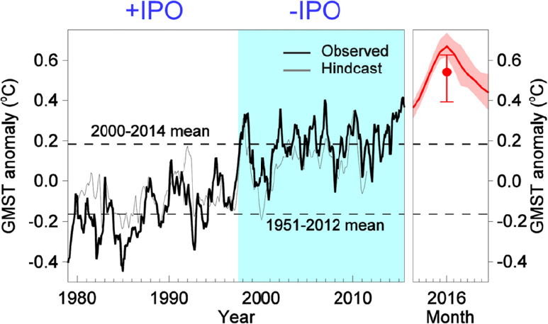
probability of a shift in the phase of the IPO generated using the Canadian seasonal-to-interannual climate forecast system (CanSIPS). Hindcasts from the forecast system match reasonably well with the observed record of the IPO, lending some confidence to the system’s ability to forecast the IPO (Figure 25). Such forecasts suggest that GMST will be about 0.4 C degrees warmer over the next year than conditions over the past 15 years (e. g., it is likely to be substantially warmer in the next year than it has been on average during the recent slowdown period).
Fyfe then used a very large ensemble of model runs to assess the probability of an IPO sign change in 2015 (after an 18-year slowdown) and in 2020 (after a 23-year slowdown). Both probabilities were low: 10 percent and 3 percent, respectively. Given average temperatures in 2015 (at the time of the workshop) and the forecast for a very warm 2016, Fyfe suggested that the current negative IPO phase ended in 2015. He then looked at the temperature response in analogs from the large ensemble and found that the recent and forecast trends are consistent with an IPO shift. Thus, Fyfe concluded that the slowdown has ended or will end very soon.
The Role of Uncertainty
Baylor Fox-Kemper of Brown University discussed the uncertainty in our understanding, observations, and modeling of air-sea exchange, and what that uncertainty implies for predicting decadal climate variability. Air-sea exchange processes at a variety of scales affect how much heat is stored in the ocean; the errors associated with this term are of a
magnitude similar to or greater than the observed slowdown. Fox-Kemper concluded that these uncertainties in the air-sea exchange rates, and consequently the global heat budget, should be reduced if we are to make robust predictions of decadal variability into the future.
The Argo array of ocean measurements provides the best available estimates of ocean heat content today. Even with these measurements, the error in the ocean heat content is very large and currently hinders any possibility of balancing global energy budgets on interannual to decadal timescales, according to Fox-Kemper. Given the huge extent and spatial variability of conditions in the ocean, many more observations are needed to decrease this uncertainty and allow for true predictability. Denser measurements, or more clever ways of interpolating the data (see also Overcoming Data Limitations), are needed, said Fox-Kemper, in order to estimate the ocean heat budget within an acceptable range of uncertainty. Similar uncertainties exist in current estimates of air-sea energy fluxes and top of the atmosphere (TOA) fluxes, and will also require more extensive observations (e. g., satellite measurements) in order to detect anomalies on these short timescales.
In stochastic modeling2 of decadal variability, predictability can arise if there are connections between regions, that is, if one region responds with a lag to well-observed conditions in another region (e. g., if the poles lead the tropics or the tropics lead the poles). Fox-Kemper said that this type of predictability likely explains why linear inverse models can exhibit some skill. Although available and useful in some contexts, stochastic modeling offers little support for the ability to make dynamical predictions in novel regimes. In order to make progress on dynamical decadal prediction, parameters must be better known than at present (or better data-assimilation techniques must be applied) and currently unparameterized processes, particularly those affecting air-sea fluxes, must be represented. Fox-Kemper also noted that moving toward really useful decadal climate prediction would require a change of culture and orientation in the research community from exploration to operational forecasting (including the designation of forecast skill scores, validation, etc.).
Veronica Nieves explained that predicting GMST over the next two decades will require determination of the fate of heat that has been stored in the Pacific and Indian Oceans as a result of planetary warming. Some of this heat is already emerging toward the surface, which will drive GMST rise. One important question is whether some of the trapped heat will be absorbed into the deeper layers of the ocean and how that might affect global temperatures in the future. So far, there is not yet any observational evidence of large amounts of heat below 300 m, according to Nieves.
___________________
2 Stochastic modeling is used to estimate probability distributions of potential outcomes by allowing for random variation in one or more model input over time.


