
Model Configuration
Model configuration includes the specification of the spatial and temporal scales of the model, the state variables to be tracked, and what processes are included and how they are represented.
General Comments
4. The temporal and spatial scales of the SAV and FD models are reasonable but the representativeness of selected reaches and the variance properties associated with the use of QUAL2E outputs as model inputs should be clearly documented.
The temporal and spatial scales of the FD and SAV models should be defined based on the key aspects of the driving variables (e.g., flows), the rates of the processes to be simulated, and the questions to be addressed. In addition, the temporal and spatial scales need to be compatible. For the FD model, an hourly time step and 1 m2 cells are reasonable decisions, although the spatial resolution seems relatively fine compared to the time step. Fish trying to forage, avoid predators, or prevent localized overcrowding can move potentially many cells in one hour. The movement algorithm needs to be capable of dealing with realistic distances moved in a time step. For the SAV model, daily time steps and 1 m2 cells are reasonable, although permitting colonization only once per month may not capture lateral growth of these clonal plants. Using daily averaged values of flow as a forcing for the SAV model is likely adequate for simulating depth and light availability, but may not permit incorporation of additional mechanisms related to flow such as uprooting or dispersal.
Model inputs include the hydraulics and water quality outputs from the QUAL2E model, with the FD model also receiving inputs from the SAV modeling. Collapsing the resolution of the two-dimensional (2-D) grid of QUAL2E from 0.25 m2 to 1 m2 cells was a reasonable decision by the development team; care should be taken in how the predictions of the QUAL2E are aggregated. The QUAL2E modeling also has a fast time step so its results can be summarized to match the hourly time step of the FD. Whenever aggregations are done, it is advisable to keep track of the loss of variance in the transferred variables (e.g., hourly variations around a daily average flow; value of 4 cells to one value for the larger cell) and whether different aggregation schemes (snapshot versus averaging versus daily minimum) affect the values of the transferred variables.
The spatial domain of the FD model is not simply the area that encompasses the number of FD individuals (abundance) expected in their entire geographic range. Rather, the FD model simulates individuals in certain reaches (subregions) of the system affected by the HCP. How well these subregions, simulated independently, represent the area inhabited by the entire FD population should be confirmed. (This issue of the representativeness of regions was discussed extensively in Chapter 4 of NRC, 2015.) For the SAV model, simulations at the reach scale are useful for predictions of HCP-related effects and also for model validation purposes.
Fountain Darter
5. The use of an individual-based approach imbedded within a 2-D spatial grid for full life-cycle simulations of FD population dynamics is a scientifically sound framework for the questions being asked, but there remain some important steps to link the FD dynamics to their habitat.
The parallel development of the FD and SAV modeling has advantages in that adjustments can be made in each to ensure both models are configured to allow accurate transfer of habitat information from the SAV to the FD models. It is planned that the FD model will require the output of the SAV model but the SAV modeling is not affected by the dynamics of FD. Currently, the FD model is not using results of the SAV modeling as inputs of habitat; rather the FD model is using inputted field data-derived habitat maps that abruptly update every six months (uncoupled mode). This is a reasonable temporary fix in order for the development of the FD model to continue while the SAV modeling gets refined. However, because the uncoupled approach uses observed SAV maps, habitat in the FD model is not directly linked to flow. Therefore, the uncoupled version, in its present form, cannot be used to examine HCP-related scenarios involving changes in flow. The coupling of the SAV and FD models are discussed below.
6. The representation of the processes of FD growth, mortality, reproduction, and movement presently in the model are well-founded but may be too simple and not sufficiently linked to changes in habitat and flow to answer some of the important management questions.
Growth is presently represented as fixed in the FD model. That is, stage durations determine the progression from one life stage to the next, and these durations do not vary within or between simulations. Thus, the approach implicitly includes growth rate of individuals but body length or weight are not tracked as state variables. Sometimes this approach is misinterpreted as assuming that food is not limiting. The degree of food limitation is determined by how the durations are estimated; if estimated from the field and food was limiting in the field conditions, then the durations reflect highly averaged but still food-limited conditions. However, the fixed-stage duration approach does make the strong assumption that the availability of food does not vary much from the conditions under which the durations were determined. The present version of the FD model assumes that individuals will obtain the food needed to achieve the growth rates dictated by the durations, and these growth rates do not vary much in space, seasonally, based on the specific habitat being inhabited, or based on flow. Thus, the ability for growth of individual FD in the model to respond to variation in environmental and habitat conditions, including HCP-related actions, is very limited. The biological realism of this limitation, and how it affects the usefulness of the model, should be evaluated.
Mortality is represented as stage-specific rates plus additional rates dependent on temperature and movement. The movement-related mortality rate is triggered when the number of movement time steps (24 per day) that an individual spends in open water or without options to move to other less crowded vegetated cells is exceeded (see Movement paragraph below). When an individual dies, it is removed from the simulation. This representation of mortality related to movement being density-dependent is critical because it is the only source of density-
dependent control on the FD population within the model. It only operates at relatively high FD abundances (so no depensatory mortality is represented) and it only occurs when SAV habitat is limited relative to FD densities. The role of flow is, at best, an indirect effect through flow affecting SAV; however, such dependence of SAV on flow is not presently in the FD model.
Reproduction is relatively fixed in the FD model, with maturity dictated by the fixed stage durations until the adult stage and fecundity fixed at 19 eggs per batch per female. The aspect of reproduction that can vary is based on vegetated cells. This is because if a female is attempting to spawn, the individual must be in a vegetated cell and must not have spawned for at least a month. When these two conditions hold, there are fixed probabilities by month that the individual will spawn and release 19 eggs. Eggs remain in the cell into which they were released as they progress to larvae and then to juveniles; juveniles and adults can move. Reproduction has the potential to be related to habitat and to be density-dependent. For example, if SAV is severely limiting as habitat for FD, then female individuals that could spawn based on the other constraints may not spawn because of the limited availability of vegetated cells. It is not clear how this would occur in the model (e.g., would individuals move to vegetated cells for reproduction?) and whether such severely limiting habitat conditions are realistic.
Movement is a rule-based neighborhood search approach, and it is only triggered under locally crowded conditions. NetLogo® follows individuals in continuous space, and after an individual moves and its position is updated to its new continuous location, the cell that the individual is located in is then determined. The cell location determines the environmental conditions an individual will experience for the next time step. The present version uses a cell-by-cell movement rather than using conditions to determine the x and y velocities of individuals and then updating their continuous locations. The present movement algorithm also uses up to 24 evaluations in a day, which can be confused as being hourly. However, this is not the case because conditions affecting movement do not change hourly but rather change daily (depth, velocity, temperature) or seasonally (vegetation type). The time-stepping of movement within the day is to deal with individuals moving for a day among very small cells (1 m2) and to allow some exploration by the individual of the local area. An alternative would be to update movement only once per day but to allow an individual to “see” a larger neighborhood than one cell in the four (or eight) directions.
The movement rules are driven by maximum FD densities that are assigned to the vegetation types for each cell that then change seasonally. Movement is triggered when the FD densities in a cell exceed the maximum densities. Some movement between adjacent cells even if the present cell is not too crowded is included: if an adjacent cell is also less than maximum density, then there is a 50/50 chance to move there or stay in the presently occupied cell. In the other case of overcrowding in a cell, the individual attempts to move to a neighboring vegetated cell and only can if that cell is not crowded. If all vegetated adjacent cells are also crowded, then the individual would move to an adjacent water cell if there are any. The number of times the individual is in water cells is accumulated and used to determine death (too many time steps in water cells leads to death). An individual can also die if no uncrowded or water cells are available to move into for enough time steps.
Use of a rule-based movement implemented on a cellular (cell to cell moves) scale can realistically represent movement. The difficulties arise when the temporal and spatial scales are not well matched. The approach taken with the FD model to address this potential issue of a coarse (daily) time step with a fine (1-m2) spatial resolution is to allow for 24 moves within each day. Information on the typical distances moved by individuals and plotting of the Lagrangian
trajectories of individuals under different vegetation and flow conditions should be presented to confirm the realism of the simulated movement behavior. Another potential difficulty with a cellular approach to movement is if the spatial resolution of the FD grid is changed – movement to a cell now involves traveling a different distance in the same time step. Finally, there is always debate with a neighborhood search algorithm about what do the individual fish sense and how do they know how to go a neighboring cell without having visited it. The fine spatial resolution of the FD model helps in this case because it is easier to envision individuals detecting gradients and other cues on 1-m2 basis that would allow them to “sense” the conditions of the destination cell in advance of moving there.
The only linkage among the growth, mortality, reproduction, and movement processes is how movement can contribute to mortality. This may be reasonable for FD and the questions being asked but it very important for the audience to understand this so the results can be properly interpreted and the model used appropriately. Growth is fixed and based on specified durations of life stages; no matter what conditions are simulated, the individuals will always grow at the same rates and progress through the life stages at the same rates. Mortality does not depend on size but only on stage and temperature. Reproduction, which like mortality is often represented as size-dependent in fish population models, is completely size-independent in the FD model. Maturity depends on stage, which depends on growth, which is fixed; fecundity is also fixed per individual. For these reasons, interpretations of modeling results such as “flow caused slower growth and this lead to higher mortality and lower reproduction” are impossible. The point is that interpretation of model results and the types of scenarios that can be simulated depend on the structure of the model. In the FD model, few of the possible linkages (see Rose et al., 2001) between growth, mortality, and reproduction are represented. This may be appropriate—it depends on the biology of the species—but is atypical of many individual-based and population models of fish and requires careful consideration as modeling results are reported and interpreted.
7. Thresholds in process representations should be used cautiously because they can erroneously create non-linear population responses and unrealistic sensitivities to changes in habitat and flow.
The use of daily maximum and minimum values from QUAL2E as inputs to the FD model should be done carefully. If processes are formulated to depend on maximum or minimum daily values (e.g., minimum dissolved oxygen [DO] affects daily mortality), then the model is internally consistent. However, such formulations should be done cautiously, especially with the relatively smooth changing hourly values of the rest of the processes in the model. One of the advantages of the individual-based approach is that it allows accumulation of hourly exposure of individuals to environmental conditions over time. While using minimum or maximum daily values for each day to affect processes is mathematically valid, formulating how these minimum and maximum values affect processes, which themselves could be a threshold response (rates change suddenly not smoothly), is challenging. At a minimum, a thorough sensitivity analyses to evaluate the impact of these thresholds seems warranted. The link from flow to temperature and DO is important because these indirect effects of flow are the only effect of flow on FD to date in the FD model. Thus, interpreting how alternative flows affect FD using the FD model requires understanding how changes in flow affect velocities and depth that are then used as input to the
QUAL2E model, and then how these changes in hydraulic outputs affect QUAL2E’s predictions of maximum daily temperature and minimum daily DO.
The use of observed densities for maximum FD densities by vegetation type acts to smooth over the threshold effect of capping FD densities by vegetation type. The smoothing occurs because a range of “maximum” densities are used for each vegetation type rather than a single value. A possible inconsistency occurs because observed densities are not truly maximum densities. Nonetheless, the use of observed densities for maximum densities will help in calibration; that is, as SAV types change in the FD model, the maximum densities change, which in turn encourages the model-predicted densities to mimic the observed densities. Total abundance of FD is the sum of their densities over all cells; thus, model-predicted abundance is a direct result of what values the maximum densities are set to. Because the observed densities were used to limit the model and then the calibration and validation use the sum of the simulated densities compared to the sum of the observed densities, the calibration and validation results showing good agreement is not as rigorous as it may seem based on the predicted versus observed abundances plots. This calibration strategy requires some skill because exceeding the specified maximum densities triggers movement, which can result in higher mortality. Proper interpretation of the calibration and validation results is critical for associating the appropriate level of confidence with model predictions of HCP effects.
8. The representation of density-dependence and how its effects on individuals manifest at the population level needs further evaluation.
Density-dependence is when the rates of a process (e.g., mortality) depend on the number of individuals present in a specified area (e.g., particular cell). Density-dependence can occur with growth, mortality, reproduction, and movement (Rose et al., 2001). As with other effects (e.g., flow), density-dependent effects on mortality and reproduction directly affect the number of individuals in the population (abundance). Density-dependent growth and movement are important because they can have indirect effects on mortality or reproduction (e.g., mortality rate decreasing with size); otherwise, changes in growth or movement do not affect abundance. Including density-dependence in population models is important because most density-dependent effects are a negative feedback and act as compensatory mechanisms. They will offset some of the response of the population to changes in habitat and other factors. For example, a decrease in spring flow can cause reduced SAV habitat for FD and increases their mortality rate because of less cover resulting in increased predation. However, the reduction can then be offset to some extent by reduced crowding at spawning, resulting in females releasing more eggs and these having higher survival. Thus, even with fewer spawners, the higher individual fecundity and higher egg survival results in an increased total egg production. (Note: such a logic chain of responses is not possible in the current version of the FD model.) In subsequent years, the reduction in the population is less than what would be expected from the reduced habitat alone under density-independence. Similarly, augmenting habitat would result in less positive response than expected under density-independence. Without density-dependence (no negative feedbacks), populations cannot be stable for extended periods of time because slight changes in reproduction or mortality must result in them either going extinct or growing unbounded.
The representation of density-dependence in the FD model is limited and restricted to increased mortality under relatively extreme local crowding. Each cell is assigned a habitat type and a maximum density is generated from field data on densities. Increased mortality occurs
when movement options are limited to neighboring cells that are also at their capacity. While this triggering of density-dependence when certain crowding conditions occur is a reasonable representation, it is quite limited in scope. There are other aspects of mortality, as well as growth and reproduction, which could be density-dependent. A simple approach that would allow rapid exploration of the importance of density dependence would be to assume that survival, growth, or fecundity decrease a reasonable amount (similar to the range exhibited in data) as density goes up (depending on vegetation type). Simulations with various combinations of the possible density-dependent processes could be analyzed to determine if further effort to refine the relationships is warranted. In general, a clear rationale for what processes are density-dependent—based on the data, expert opinion, and other similar species—should be developed.
However density-dependent is represented, when all effects are simulated on individuals it is important to show how these effects add up to density-dependence mortality at the population-level. For example, a typical diagnostic to use is showing the annual spawner–recruit plot that results from multiple years of simulation. A common measure of spawners is total eggs produced in a year, and a common measure of recruitment would be the number of individuals that survived from those eggs to become juveniles and then to become adults. This can be difficult with a species like FD that spawns all year long and for which the present formulation includes density-dependence in the adult stage; defining over what months to sum egg production and how to accumulate recruits to obtain annual values needs to be considered. In addition, because of its potential importance on population dynamics, the density-dependence in adults should also be characterized and quantified. Based on the life history of the FD, one would expect a Beverton-Holt type spawner–recruit relationship, likely with a weak response (gradually leveling off curve, Figure 1B). One often characterizes these curves with the steepness coefficient that summarizes the strength of the density-dependence in the spawner-recruit relationship, which has been reported for hundreds of fish species (e.g., Rose et al., 2001). Based on the Committee’s experience, a steepness value of 0.5 to 0.7 is anticipated. One could also try to create a spawner–recruit curve using proxies from the field data and compare its properties (e.g., shape) to the model predictions. Some additional exploration of how density-dependence manifests itself at the population-level is needed.
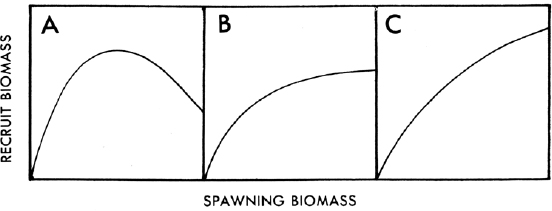
SOURCE: Figure 10 from Parrish and MacCall (1978).
9. The representation of flow effects in the model seems too limited in potential effects due to reliance on having site-specific empirical evidence for the effects.
A logic flowchart showing how a change in spring flow affects FD directly and indirectly would be helpful. It must start with flow and eventually result in affecting mortality or reproduction, as these are the two processes that determine FD abundance. Flow effects on growth or movement must then continue in their logic to see how these flow-related changes affect mortality or reproduction. For example, if lower flow affects water depth in cells and this causes FD to move to other cells but their growth, mortality, and reproduction are the same in the new cells, then the lowered flow had no effect on FD abundance despite movement being density-dependent. Similarly, if lower flow was represented as affecting growth rate (i.e., longer or shorter stage durations), this also would have no effect on FD abundance unless mortality rate also was specified as dependent on stage duration. In the present model, mortality rate decreases with stage and thus prolonged duration in early life stages, with their high mortality rate, could result in higher cumulative mortality. Slowed growth could also result in delayed maturation (reaching the adult stage) and reduced fecundity but these may or may not have ecologically meaningful effects on population. The logic becomes complicated; does flow affect temperature which then affects mortality or does flow affect SAV, which affect FD habitat? A logic flowchart would enable easier tracking of the direct and indirect effects of changes in flow or other variables affected by the HCP.
With the present configurations of the SAV and FD models, the direct and indirect effects of flow on FD seem to be limited. The direct effects are limited to how flow affects daily maximum temperature and minimum daily DO (from QUAL-2E), both of which affect mortality rates. Flow can also indirectly affect FD through flows effects on SAV dynamics, which determines the maximum FD densities in cells, which could lead to movement that causes increased mortality rates. In the uncoupled mode, the observed spatial maps of SAV reflect the effects of flow, but flow is not available to be adjusted in any systematic way (i.e., there is no flow input variable to the SAV maps). When the SAV model is further along in development and the coupled mode is implemented, any indirect effects of flow on FD through SAV will depend on how flow affects the SAV. Present plans, which are subject to adjustment and change as the SAV modeling proceeds, suggest flow could affect the biomass of an SAV species in a cell by altering water depth, which determines light limitation of photosynthesis and temperature affecting respiration. The report also lists velocity directly affecting SAV, but its role it not yet clear. It also has been proposed that the way an SAV species is assigned to a cell (transition) every three months, and maybe also dispersal, could depend on flow, although these remain ideas at this point.
Model development can proceed using several different philosophies, and the approach seemingly taken for the FD model may have over-restricted how flow effects are represented. One philosophy (“top-down”) is to focus on formulating the model so that there are relatively few parameters that can then be optimized based on simulated and observed population-level variables (e.g., adult abundance over time). Here the fit between predicted and observed values is critical and the idea is avoid over-specification of the model. Another philosophy (“bottom-up”) is to carefully develop each component of the model so that when they are put together there is high confidence in the simulated population-level dynamics. The present version of the FD model relies on there being strong empirical evidence for flow effects in order for those effects to be included. In very well-studied systems, this is effective because the major possible effects
usually have been studied and their representations have a sound empirical basis. However, this approach can lead to over-simplified representations of the effects where the empirical evidence is not strong enough to justify including many of the possible effects that are suspected (e.g., intuitive, data suggestive, occur in other systems) but not documented. Thus, uncertainty due to the lack of site-specific data leads to ignoring possibly important effects. While this system is well-studied in some respects (sampling of FD densities; observational data), many would consider it under-studied in terms of process studies, especially those that relate flow to growth, mortality, reproduction, and movement of FD by life stage. Thus, the FD model reflects what is clearly known about flow effects but likely is missing other effects because of lack of site-specific measurements to justify their inclusion in the model.
There are several approaches for dealing with the possibility of under-studied effects not being considered in models. An excellent use of the FD model would be to add some of these suspected effects and explore how including them would affect model results. One approach is to use information from similar species and other systems to infer, in this case, possible flow effects on growth, mortality, reproduction, and movement. These can be put into a category that distinguishes them from the effects documented using site-specific data so people know there is higher uncertainty (less site-specific evidence) with these effects. One can then use a series of simulations (like a sensitivity analysis) to see if these less-well-known effects could have significant population-level effects and have an impact on the advice provided to management. This use of the FD model also then leads to the identification of uncertain information that is also critical to accurate predictions and how to design sampling or experiments to provide this information on a site-specific basis for later incorporation into the FD model.
Submersed Aquatic Vegetation
10. Use of highly simplified formulations describing nutrient limitation or effects of temperature on photosynthesis may be problematic when the model is applied to scenarios where these factors are critical.
Model development must necessarily simplify the system. Nonetheless, it is critical to document and justify what assumptions and decisions have been made regarding which mechanisms to include or focus on. This justification should explain why certain factors or processes were included and why they were formulated at the level of detail used, as well as state why some factors and processes were not included. To develop an SAV model without considering the impacts of nutrients, as this model does, is highly unusual. It was the recommendation of the Committee’s first report (NRC, 2015) that nutrients be measured regularly. Nutrients can be both limiting to plant growth and also can result in impaired growth conditions. At low flow conditions, especially in the lake systems that can act as refuges, there could be a future scenario where nutrient issues may be critical. For example, abundant nutrients under low flow conditions may encourage growth of epiphytes that then limit light availability to the SAV. For a model such as this, which is being developed largely to help predict the response of the system to hydraulic conditions not regularly experienced, it seems critical to systematically evaluate the basic factors involved in the growth of the SAV for potential inclusion in the model, level of detail of representation if included, and possible mechanisms linking them to flow.
The treatment of temperature in the model is inconsistent in that there is no temperature limitation in the photosynthesis formulation, but temperature effects are included in respiration and growth equations. Including a temperature limitation term for photosynthesis would resolve these inconsistencies. In many instances, respiration and photosynthesis respond differently to temperature changes and explicitly including temperature dependencies may be illuminating.
11. In general, more model detail in the final report is critical for both review and future users of the SAV model.
The SAV modeling group has been very helpful in answering questions related to the BIO-WEST (2015) report. Nonetheless, future reports should provide more detail on decisions and assumptions, choices for parameterization, and occasionally referencing of the other coupled models (FD and water quality) in order to aid future users and developers of the SAV (and FD) models. For example, providing greater clarity on the conversions from grams dry weight to glucose and back again, and detailing differences in these conversions amongst species, is important. The Committee’s reading of the BIO-WEST (2015) report suggests that light attenuation data are lacking, such that gathering some field data for solar irradiance and light attenuation would improve upon current forcings and fixed parameterization of the k value (light extinction coefficient). The BIO-WEST (2015) report also suggests that basic temperature limitation studies are not in abundant supply for the varied species modeled here and that the impact of temperature on mortality is not strongly understood. Providing referenced literature on these links (e.g., between mortality and temperature) is recommended, as is providing more detail on the relationship between flow and scour. Finally, details on model initialization should be included in the final model description. It would be most effective for the modelers themselves to provide an explicit list of the assumptions made, perhaps in some prioritized list, to aid in future iterations and improvements to the model. The developers have the clearest picture of what data, research, and questions must be pursued to improve future management of the systems and to aid in improvement of the models. Strongly identifying those areas where assumptions were made or data were lacking is an invaluable practice.
12. Many parameters appear calibrated, and it is not clear how the values of fixed parameters are connected to literature values. Formulations are taken from a crop model, which is not a problem as long as the developers sufficiently incorporate SAV morphology, growth, and physiology in the formulations and parameterization. Describing how the calibration is done and convincing end users that the parameterization is appropriately matched to reasonable values from the empirical literature will aid model credibility.
Calibration allows for changes in model parameters until predicted and observed values appear consistent with each other. However, calibration must also include documentation that the tuned parameters are realistic and, wherever possible, match literature and site-specific values. There is little information provided regarding parameterization in the BIO-WEST (2015) report. After some evaluation, the modeling team decided to develop a new model, based on a suite of existing models. The basic growth formulations are borrowed from Teh (2006), which focused on crop models. Using growth formulations from other plants is a common approach used by modelers and is effective and efficient as long as the formulations are carefully checked and adjusted based on SAV information and site-specific information. The model is likely extremely


