D

Stochastic Models of Uncertainty and Mathematical Optimization Under Uncertainty

This appendix provides more formal definitions and descriptions of aspects of the two key areas of prescriptive analytics, namely stochastic models of uncertainty and mathematical optimization under uncertainty, which are intimately connected. These descriptions also illustrate examples of mathematical prescriptive analytics methods that have been developed and successfully applied to address policy issues and problems associated with workforce management, skill and talent management, and human capital resource allocation in the private sector, which are analogous to the type of prescriptive decision-making policy issues and problems related to missions of the Office of the Under Secretary of Defense (Personnel & Readiness), referred to as P&R, including recruiting, training, retention, optimal mix, readiness, staffing, career shaping, and resource allocation. Although there are unique considerations for the Department of Defense (DoD), an understanding of these and related large-scale efforts in the private sector is an important starting point. Then policy issues and problems related to P&R missions can be investigated through variations of such methods, coupled with DoD data.

The following descriptions are highly mathematical, relative to the rest of this report, and will likely be relevant to only a subset of readers. However, the committee believes these examples may be helpful to analysts trying to implement these methods.

STOCHASTIC MODELS OF UNCERTAINTY

To illustrate some of the concepts described in Chapter 4, two examples of stochastic models of uncertainty involved in decision-making problems related to P&R are presented. The first example concerns trade-offs among skill capacities and readiness of resources given uncertainty around the demand for such resources, which relate to P&R missions associated with optimal mix, readiness, staffing, and resource allocation. This material is based on the works of Bhadra et al. (2007), Cao et al. (2011), Jung et al. (2008), Jung et al. (2014), and Lu et al. (2007), where additional technical details can be found. The second example concerns trade-offs among the evolution of capabilities and readiness of personnel resources over time given uncertainty around time-varying supply-side dynamics, which relate to P&R missions associated with recruiting, training, retention, optimal mix, readiness, staffing, career shaping, and resource allocation. This material is based on the work of Cao et al. (2011), where additional technical details can be found.

Example: Stochastic Loss Networks

One such example is based on the use of stochastic loss networks to model the probability of sufficient capacity and readiness of resources given uncertainty around the demand for such resources, as well as the interactions and dynamics of resources across different projects and tasks. As a specific illustrative instance related to P&R, analogous to the workforce application studied in Cao et al. (2011), consider the problem of determining the likelihood of not having enough resources of type i ∈ I (e.g., experienced aircraft mechanics) in order to satisfy the demand for projects of type k ∈ K (e.g., sustaining high aircraft mission-capable rates), where I denotes the set of resource types and K denotes the set of project types. Let A_i,k denote the amount of type-i resources that are required to deliver type-k projects and C_i the total amount of type-i resources available. The demand for type-k projects is modeled as a stochastic arrival process with rate v_k (derived from the output of predictive analytics)—that is, the times between the need to deliver type-k projects follow a probability distribution with mean v_k^–1. When delivery of a type-k project is needed and the amount of type-i resources available for deployment at that time is at least A_i,k for all i ∈ I, then the type-k project is delivered and the required resources of each type are deployed for a duration that follows an independent probability distribution with unit mean (without loss of generality); otherwise, the type-k project cannot be delivered and the opportunity to do so is said to be lost. Define L_k to be the stationary loss-risk probability for type-k projects

and n_k the number of active type-k projects in equilibrium, with n := (n_k). By definition, we have n as an element of the space of possible deployments

where A := , C := (C_i), and ℤ₊ denotes the set of non-negative integers. Assuming independent Poisson arrival processes with rate vector v = (v_k), the key probability measure of interest then can be expressed as

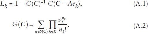
where e_k is the unit vector corresponding to a single active type-k project. Refer to Jung et al. (2008) and Jung et al. (2014) for additional details.

Although the expressions above provide an exact solution for L_k, the complexity of computing this solution is likely intractable (as the problem is known to be #P-complete¹), making it prohibitive for practical problem sizes related to P&R missions within DoD. To address this issue, from the analysis and results in Jung et al. (2008) and Jung et al. (2014), the key probability measure can be accurately estimated as

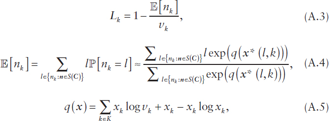
where [^.] denotes the expectation operator, [Y] denotes the probability of event Y, x := (x_k) is a continuous relaxation of n defined over a continuous relaxation of the space of possible deployments S(C) and subsets of this relaxation, ₊ denotes

___________________

¹ #P-complete is a computational complexity class that defines a problem to be #P-complete if and only if it is in #P and every problem in #P can be reduced to it by a polynomial-time counting reduction, that is, a polynomial-time Turing reduction relating the cardinalities of solution sets (Valiant, 1979).

the set of non-negative reals, , and x*(l,k) is the mode of the distribution associated with . Corresponding results under general renewal arrival processes can be found in Lu et al. (2007) and Cao et al. (2011).

Example: Time Inhomogeneous Markov Processes

Another example is based on the use of discrete-time stochastic processes to model the evolution of capabilities and readiness of personnel resources over time, given uncertainty around the time-varying supply-side dynamics with personnel acquiring skills, gaining experience, changing roles, and so on; some attrition of personnel; and new personnel being introduced. As a specific illustrative instance related to P&R, analogous to the workforce application studied in Cao et al. (2011), consider a time inhomogeneous Markov process of the evolution of personnel resources over a finite horizon of T + 1 periods in which resources are aggregated into groups based on combinations of attributes of interest (e.g., rank, skill, experience, proficiency). Let J denote the family of all such possible combinations of attributes of interest for personnel resources. The time inhomogeneous Markov process is then defined over the state space of all possible numbers of resources that can possess each combination of attributes composing J, namely

where m := (m₁, …, m_|J|) and M := (M₁, …, M_|J|), with M_j ≤ ∞ as an upper bound on the maximum number of resources possible in group j ∈ J. Define y(0) := (y₁(0), …, y_|Ω|(0)) to be the initial distribution and K(t) the Markov kernel for time t ∈ {0, …, T}. The kernels K(^.) incorporate the probabilities governing all transitions between states in Ω from one period to the next (derived from the output of predictive analytics), including introduction of new personnel, attrition of existing personnel, acquisition of skills, promotion in rank, gain in experience, and so on. Then the distribution (probability measure) of this time-inhomogeneous Markov process at time t is given by

where y_k(t) represents the probability of being in state k ∈ Ω at time t ∈ {1, …, T} given the starting distribution y(0).

Due to the combinatorial explosion of the size of the state space Ω, an

exact analysis is prohibitive for all but very small values of |J| and M_j. To address this so-called curse of dimensionality, one can consider a type of fluid limit scaling of the time-inhomogeneous Markov process that instead records the expected number of resources in each group, thus rendering a single state for each group of attributes. For each state j ∈ J and t ∈ {0, …, T}, define y_j(t) to be the expected number of resources in state j at time t, ι_j(t) the expected amount of new introductions into state j over [t, t + 1), and α_j(t) the expected amount of attrition from state j over [t, t + 1), with y(t) := (y_j(t)), ι(t) := (ι_j(t)), and α(t) := (α_j(t)). Further define p_jj′(t) to be the stationary probability of transitions from state j to state j′ over [t, t + 1), where Σ_j′∈_J p_jj′(t) ≤ 1. When state j attrition is positive, this inequality is strict and 1 – Σ_j′∈_J p_jj′(t) represents the stationary probability that a resource leaves state j through attrition, such that α_j(t) = y_j(t)(1 – Σ_j′∈_J p_jj′(t)). The evolutionary dynamics of this time-inhomogeneous Markov process then can be expressed as

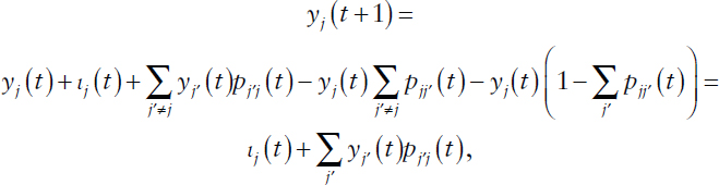
or, in matrix form (using row vector notation),

where P(t) := [p_jj′(t)], ∀j,j′ ∈ J, and ∀t ∈ {0, …, T}. Additional algebra yields

The experience reported in Cao et al. (2011) suggests the accuracy of this solution to be within a few percentage points in predicting the evolution of capabilities and readiness of personnel resources for large organizations with many thousands of resources over horizons of a year or so.

MATHEMATICAL OPTIMIZATION UNDER UNCERTAINTY

A more formal definition and description of mathematical optimization under uncertainty is presented, followed by a few examples of such methods involved in decision-making problems related to those of P&R.

In the case of one-time decisions over a given time horizon, a general formulation of a single-period decision-making optimization problem can be expressed as

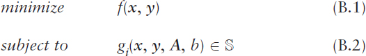
where x := (x₁, …, x_n) is the vector of decision variables, y := (y₁, …, y_m) is a vector of dependent variables, f : ⁿ → is the objective functional, g_i : ⁿ → is a constraint functional, i = 1, …, k, A is a matrix, b is a scalar, and is the constraint region. The objective functional f(^.) and constraint functionals g_i(^.) define the criteria for evaluating the best possible results, while the vector y, the matrix A, the scalar b, and the constraint region are based on the stochastic models of the system of interest. The relationships among these components of the optimization formulation are critically important and often infused with subtleties and complex interactions. Of course, the objective in (B.1) can be equivalently formulated as a maximization problem with respect to –f(^.).

When the variables in (B.1), (B.2) are deterministic (e.g., a point forecast of expected future demand), then the solution of the optimization problem (B.1), (B.2) falls within the domain of mathematical programming methods, the details of which depend upon the properties of the objective functional f(^.) and constraint functionals g_i(^.) (e.g., linear, convex, or nonlinear objective and constraint functionals) and the properties of the decision variables (e.g., integer or continuous decision variables). On the other hand, when the variables in (B.1), (B.2) are random variables or stochastic processes (e.g., a distributional forecast of future demand or a stochastic process of system dynamics), then the solution of the optimization problem (B.1), (B.2) falls within the domain of mathematical optimization under uncertainty methods, the details of which again depend upon the properties of the objective functional f(^.) and constraint functionals g_i(^.) and the properties of the decision variables.

In the case of adaptive decision-making policies for dynamic adjustments to decisions and actions throughout the time horizon as uncertainties are realized, a general formulation of a multiperiod decision-making optimization problem can be expressed as

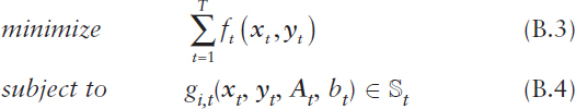
where x_t := (x_1,t, …, x_n,t) is the vector of decision variables for time t ∈ {1, …, T}, y_t := (y_1,t, …, y_n,t) is a vector of dependent variables for time t, f_t : ⁿ → is the objective functional for time t, g_i,t : ⁿ → is a constraint functional for time t, i = 1, …, K, A_t is a matrix, b_t is a scalar, _t is the constraint region for time t, and T is the time horizon. The objective and constraint functionals f_t(^.) and g_i,t(^.) define the criteria for evaluating the best possible results, while the vectors y_t, the matrices A_t, the scalars b_t, the constraint regions _t, and time horizon T are based on the stochastic models of the system of interest. The relationships among these components of the optimization formulation are critically important and often infused with subtleties and complex interactions. Of course, the objective in (B.3) can be equivalently formulated as a maximization problem with respect to –f_t(^.).

When the variables in (B.3), (B.4) are deterministic (e.g., a point forecast of expected future demand over time), then the solution of the optimization over time problem (B.3), (B.4) falls within the domain of mathematical programming and deterministic dynamic programming and optimal control methods, the details of which depend upon the properties of the objective functionals f_t(^.) and constraint functionals g_i,t(^.) (e.g., linear, convex, or nonlinear objective and constraint functionals) and the properties of the decision variables (e.g., integer or continuous decision variables). On the other hand, when the variables in (B.3), (B.4) are random variables or stochastic processes (e.g., a distributional forecast of future demand over time or a stochastic process of system dynamics over time), then the solution of the optimization over time problem (B.3), (B.4) falls within the domain of mathematical optimization under uncertainty and stochastic dynamic programming and optimal control methods, the details of which again depend upon the properties of the objective functionals f_t(^.) and constraint functionals g_i,t(^.) and the properties of the decision variables. In addition, a filtration F_t is often included in the formulation to represent all historical information of a stochastic process up to time t (but not future information), where both the decision variables x_t and the system are adapted to the filtration F_t.

To illustrate aspects of the points noted above and described in Chapter 4, a few examples of mathematical optimization under uncertainty involved in decision-making problems related to those of P&R are presented. The first example concerns trade-offs among skill capacities and readiness of resources given uncertainty around the demand for such resources, which relate to P&R missions associated with optimal mix, readiness, staffing, and resource allocation. This material is based on the works of Bhadra et al. (2007), Cao et al. (2011), Jung et al. (2008), Jung et al. (2014), and Lu et al. (2007), where additional technical details can be found. The second example concerns trade-offs among the evolution of capabilities and readiness of personnel resources over time given

uncertainty around time-varying supply-side dynamics, which relate to P&R missions associated with recruiting, training, retention, optimal mix, readiness, staffing, career shaping, and resource allocation. This material is based on the work of Cao et al. (2011), where additional technical details can be found. The third example concerns trade-offs among the dynamic allocation of capacity for different types of resources in order to best serve uncertain demand, which relate to P&R missions associated with recruiting, training, retention, optimal mix, readiness, and resource allocation. This material is based on the work of Gao et al. (2013), where additional technical details can be found.

Example: Stochastic Optimization

One such example is based on optimization of stochastic loss networks to determine the best capacity and readiness of resources given uncertainty around the demand for such resources. As a specific illustrative instance related to P&R, analogous to the workforce application studied in Cao et al. (2011), consider a time horizon modeled as a stationary loss network consisting of multiple personnel resource types and multiple project types. The stochastic loss network is used to model the risk of not being able to satisfy project demand due to insufficient capacity of one or more resource types available at the time the project products need to be delivered. Define a linear base reward function with rate r_k for successfully delivering products of type k, a linear base cost function with rate c_i for resources of type i, and linear cost functions with rates for introducing, training, and retaining resources of type i, respectively.

The following formulation of a corresponding stochastic optimization problem can then be expressed as

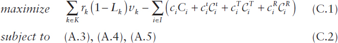
where the decision variables are the components of the capacity vector C = (C₁, …, C_I) and denote the amounts of existing, introduced, trained, and retained resources of type i with for all i ∈ I. Alternatively, (A.1) and (A.2) can be used for the constraints in (C.2) when the problem size is sufficiently small. In either case, a constraint can be added of the form L_k ≤ β_k for all k with β_k ∈ (0,1), which will tend to push the optimal solution toward increasing the resource capacities C_i in order to lower the loss-risk probabilities L_k. A nonlinear program solver can be used to efficiently compute the optimal solution to any of these

instances of the optimization problem (C.1), (C.2), possibly also exploiting the additional results in Jung et al. (2008) and Jung et al. (2014).

A time-varying, multiperiod version of the above stochastic optimization problem has also been studied. Refer to Bhadra et al. (2007) for the corresponding results and details.

Example: Stochastic Dynamic Program

Another example is based on optimization of discrete-time stochastic decision processes of the evolution of capabilities and readiness of personnel resources over time given uncertainty around the time-varying supply-side dynamics. One can start with the stochastic dynamic program formulated with respect to a time inhomogeneous Markov process whose dynamics are governed by (A.6) and where the decision variables would be based on changes in the Markov kernels K(t) that provide optimal evolution of capabilities and readiness of personnel resources. However, the combinatorial explosion of the size of the state space Ω makes the solution of such a stochastic dynamic program prohibitive for all but very small values of |J| and M_j.

Alternatively, as an illustrative instance related to P&R analogous to the workforce application studied in Cao et al. (2011), consider the optimization of decisions or actions within a fluid limit scaling of a time inhomogeneous Markov process that models the evolutionary dynamics of personnel resources over a finite horizon of T + 1 periods according to equation (A.7). Define C_j(t) to be the expected cost rate for state j ∈ J over [t, t + 1) and R_j(t) to be the expected reward rate for state j ∈ J over [t, t + 1), with C(t)= (C_j(t)) and R(t)= (R_j(t)). The expected cumulative costs and rewards of resources over the time horizon are then given by

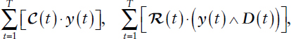
respectively, under appropriate independence assumptions, where D(t) := (D_j(t)) denotes the vector of demand for every state j ∈ J over [t, t + 1) and ∧ denotes the component-wise minimum operator (i.e., x ∧ y := min{x, y}); here the assumption is made that rewards are accrued up to the minimum of the amount of resources and the demand for such resources.

Equation (A.7) can be rewritten into the following discrete-time linear dynamical system recursion (using column vector notation):

where B(t) captures the sparsity patterns of P(t), and u(t) denotes the vector of decision variables for actions related to transitions between states (e.g., training and promotion) and for actions to introduce and retain personnel. Define P(t) := [R(t) ^. (y(t) ∧ D(t))] – [C(t) ^.y(t)]. Then the formulation of a corresponding stochastic optimal control problem can be expressed as

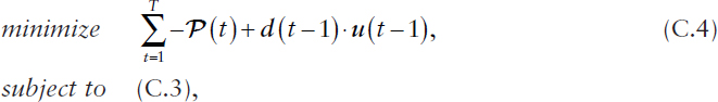
where the decision variables are u(0), …, u(T –1) and d(t) denotes the vector of expected decision cost rates for all states over [t, t + 1). Given the linear dynamical system in (C.3), the summation can be stacked in the objective function (C.4), and this optimization problem can be reformulated as a (piecewise) linear program in terms of a decision variable vector

and a weight vector

subject to the constraints (C.3) expressed in a corresponding matrix form. A linear program solver then can be used to efficiently compute an optimal solution vector z*, which yields optimal state vectors y*(1), …, y*(T) and optimal decision vectors u*(0), …, u*(T – 1).

Example: Stochastic Optimal Control

Another example is based on stochastic optimal control of the dynamic allocation of capacity for different types of resources in order to best serve uncertain demand so that expected net benefit is maximized over a given time horizon based on the rewards and costs associated with the different resource types. As a specific illustrative instance related to P&R sourcing problems, and a specific instance of the general class of dynamic resource allocation problems studied in Gao et al. (2013), consider the stochastic optimal control problem of satisfying demand (e.g., for sophisticated engineering projects) over time with two types of resources, namely a primary resource allocation option (e.g., chief engineer) that has the higher net benefit and a secondary resource allocation option (e.g., journeyman engineer) that has the lower net benefit. A control policy defines at every time t ∈ the level of primary resource allocation, denoted by P(t), and the level of secondary resource allo-

cation, denoted by S(t), that are used in combination to satisfy the uncertain demand, denoted by D(t), where S(t) = [D(t) – P(t)]⁺ with x⁺ := max{x, 0}. The demand process D(t) is given by the linear diffusion model

where b ∈ is the demand growth or decline rate, σ > 0 is the demand volatility or variability, and W(t) is a one-dimensional standard Brownian motion, whose sample paths are nondifferentiable (Karatzas and Shreve, 1991). Define the reward and cost function associated with the primary resource capacity P(t) at time t as R_p(t) := r_p × [P(t) ∧ D(t)] and C_p(t) := c_p × P(t), respectively, with reward and cost rates r_p > 0 and c_p > 0 capturing all per-unit rewards and costs for serving demand with primary resource capacity, r_p > c_p, and ∧ denoting the minimum operator (i.e., x ∧ y := min{x, y}). From a risk-hedging perspective, the risks associated with the primary resource allocation at time t concern lost reward opportunities whenever P(t) < D(t) on one hand and concern incurred cost penalties whenever P(t) > D(t) on the other hand. The corresponding reward and cost functions associated with the secondary resource capacity S(t) at time t are defined as R_s(t) := r_s × [D(t) – P(t)]⁺ and C_s(t) := c_s × [D(t) – P(t)]⁺, respectively, with r_s > 0 and c_s > 0 analogous to r_p and c_p. From a risk-hedging perspective, the secondary resource allocation at time t is riskless in the sense that rewards and costs are both linear in the resource capacity actually used.

The decision process P(t) is adapted to the filtration F_t generated by {D(s) : s ≤ t}. Any adjustments to the primary resource allocation capacity have associated costs, where I_p and D_p denote the per-unit cost for increasing and decreasing the allocation of primary resource capacity P(t), respectively. Then the formulation of a corresponding stochastic optimal control problem can be expressed as

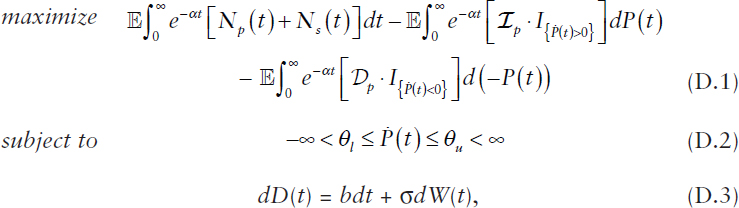
where the decision variable is the derivative of P(t) with respect to time, denoted by Ṗ(t), and where α is the discount factor, N_p(t) := R_p(t) – C_p(t), N_s(t) := R_s(t) – C_s(t), and I_{A} denotes the indicator function returning 1 if A is true and 0 otherwise. The control variable (t) is managed by the control policy at every time t subject to the lower-bound and upper-bound

constraints in (D.2), which capture the inability to make unbounded adjustments in the primary resource capacity at any instant in time. Note that the second expectation in (D.1) causes a decrease with rate I_p in the value of the objective function whenever the control policy increases P(t), and the third expectation in (D.1) causes a decrease with rate D_p in the value of the objective function whenever the control policy decreases P(t).

Suppose the per-unit cost for decreasing the allocation of primary resource capacity is strictly less than the corresponding discounted overage cost and suppose the per-unit cost for increasing the allocation of primary resource capacity is strictly less than the corresponding discounted shortage cost. Then, as rigorously established by Gao et al. (2013), the solution to the stochastic optimal control problem (D.1), (D.2), (D.3) has the following simple form for governing the dynamic adjustments to P(t) over time. Namely, there are two threshold values, L and U, with L < U such that the optimal dynamic control policy seeks to maintain X(t) = P(t) – D(t) within a risk-hedging interval [L, U] at all times t, taking no action (i.e., making no change to P(t)) as long as X(t) ∈ [L, U]. Whenever X(t) falls below L, the optimal dynamic control policy pushes toward the risk-hedging interval as fast as possible—that is, at rate θ_u, thus increasing the primary resource capacity P(t). Similarly, whenever X(t) exceeds U, the optimal dynamic control policy pushes toward the risk-hedging interval as fast as possible—that is, at rate θ_l, thus decreasing the primary resource capacity P(t). Here, the optimal threshold values L and U are uniquely determined by two nonlinear equations that depend upon the parameters of the formulation. Refer to Gao et al. (2013) for these and related results as well as for additional technical details.

REFERENCES

Karatzas, I., and S.E. Shreve. 1991. Brownian Motion and Stochastic Calculus, second edition. Springer-Verlag.

Lu, Y., A. Radovanovic, and M.S. Squillante. 2007. Optimal capacity planning in stochastic loss networks. Performance Evaluation Review 35(2):39-41.

Valiant, L.G. 1979. The complexity of computing the permanent. Theoretical Computer Science 8(2):189-201.

This page intentionally left blank.

REFERENCES

Bhadra, S., Y. Lu, and M.S. Squillante. 2007. Optimal capacity planning in stochastic loss networks with time-varying workloads. Pp. 227-238 in Proceedings of ACM SIGMETRICS Conference on Measurement and Modeling of Computer Systems, San Diego, Calif., June 12-16.
Cao, H., J. Hu, C. Jiang, T. Kumar, T.-H. Li, Y. Liu, Y. Lu, S. Mahatma, A. Mojsilovic, M. Sharma, M.S. Squillante, and Y. Yu. 2011. OnTheMark: Integrated stochastic resource planning of human capital supply chains. Interfaces 41(5):414-435.
Gao, X., Y. Lu, M. Sharma, M.S. Squillante, and J.W. Bosman. 2013. Stochastic optimal control for a general class of dynamic resource allocation problems. Pp. 3-14 in Proceedings of the IFIP W.G. 7.3 Performance Conference, Vienna, Austria, September 24-26.
Jung, K., Y. Lu, D. Shah, M. Sharma, and M.S. Squillante. 2008. Revisiting stochastic loss networks: Structures and approximations. Pp. 407-418 in Proceedings of ACM SIGMETRICS Conference on Measurement and Modeling of Computer Systems, Annapolis, Md., June 2-6.
Jung, K., Y. Lu, D. Shah, M. Sharma, and M.S. Squillante. 2014. “Revisiting stochastic loss networks: Structures and algorithms.” Preprint.