
MRIP Calibration Workshop II
Appendix 1. Detailed Implementation Steps for the Calibration Methods Proposed During the Workshop.
Summary Report: NOAA Calibration Methods Workshop - Charleston, SC
September 8-10, 2014
Lynne Stokes, Ken Pollock, Ginny Lesser
December 18, 2014
The new MRIP Access point survey has replaced the original MRFSS Access Point Survey, A variety of design changes have been made. One major consequence is that the new survey covers the fishing day more effectively than the original MRFSS Access Point Survey. Because the time series of recreational catch rate estimates form the basis of so many important fisheries stock assessments, there is the need to develop methods which "calibrate" the original time series of MRFSS estimates to the new time series of MRIP estimates. This is a difficult statistical estimation and prediction issue because both surveys were not run in parallel in any years (except for one pilot test in NC). The new estimates can be very different from the old estimates causing an abrupt change in the time series.
The purpose of this document is to outline the steps involved in implementing several model dependent calibration approaches to re-estimate catch that were discussed at the Charleston workshop. In addition, we discuss their assumptions. The first two methods use ideas of ratio estimation and assume that the major changes between the two surveys are due to a better temporal coverage of the fishing day in the new MRIP survey. The third method is a regression prediction modeling approach that will take longer to develop. None of these methods incorporate any analysis of spatial patterns or include time series methods, which might improve estimates. This would be worth exploring to determine if time series or small area estimation techniques for this short time series might provide improved estimates.
- Direct Catch Ratio Adjustment
- Steps in approach (for each subregion, state, mode, species.):
- Define peak period for each of the domains (excluding species). Peak period is defined using two criteria: 1) the contiguous range of hours during which weighted hourly proportions of total trips in the MRFSS years (prior to 2013) were greater than or equal to the corresponding weighted hourly proportions of total trips in 2013, and 2) the peak period accounted for at least 75% of the intercept data (trips) in the MRFSS years.
- Estimate peak and total catch using the 2013 data based on the MRIP survey method where both the peak and total fishing periods were sampled adequately. Denote these by cp,2013 and ctotal,2013, respectively.
- Steps in approach (for each subregion, state, mode, species.):
-
-
- Calculate the ratio R2013 = ctotal,w2013/cp,2013. This estimate and its large sample variance, based on standard Taylor series methods, can be calculated from survey sampling software packages such as SAS.
- Denote the estimator of catch based on the MRFSS method during the peak period in earlier year y(e.g,, y = 2012, 2011, etc.) by cP,y. Then the estimator of adjusted total catch for year y (i.e., a prediction of what would have been obtained if MRIP had been run) will be calculated as the product of the ratio from year 2013 and the catch for the peak period in year y; i.e.,
Ctot,y = R2013*Cp,y.
iv. The variance of the adjusted catch ctot,y can be calculated using the expression for the variance of a product of two independent random variables introduced by Goodman (1960):.
var(ctot,y) = var(R2013)(cp,y)2 + var(cp,y)(R2013)2 - var(R2013)var(cp,y)
By substituting estimates for each of the components in this equation, the variance can be estimated.
- Assumptions:
- Relative distribution of catch throughout day (i.e., between peak and total) is constant between 2013 and the year that is being adjusted for each domain
- Advantages:
- Simple to apply.
- Disadvantages:
- Information that is available for non-peak hours are not used.
- Two variations of this approach:
- Keep a fixed peak time the same (note this will vary by state and mode)
- Use different peak times (allow this to vary by state, mode and year since this was allowed to vary in these groups)
-
- Complex Ratio Method Based on Fishing Effort Distributions
- Steps in approach (for each subregion, state, mode, species etc.):
- The 2013 daily relative distribution of total fishing effort is obtained and also the relative distribution of total fishing effort data for the year to be compared to (for example, for y = 2012, 2011, etc.). Total fishing effort is estimated as the fishing effort estimate from separate telephone surveys (CFITS, FHS) that is subsequently expanded by coverage correction factors estimated from APAIS.
- Steps in approach (for each subregion, state, mode, species etc.):
-
- The 2013 sampling weights are then adjusted (up or down weighted) so that the 2013 relative distribution matches the year y relative distribution. This is to be done by using discrete temporal bins with the exact bin widths yet to be determined. The adjustments made to the 2013 sample weights are a ratio style adjustment of the form:
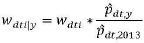
where wdti is the unadjusted 2013 sample weight for angler-trip i in time bin t in subregion, state, mode domain d,
 is the original 2013 weighted proportion for time bin t of total trips in domain d,
 is the year y weighted proportion for time bin t of total trips in domain d, and
wdti|y is the 2013 sample weight for angler-trip i in time bin t in domain d adjusted to year y.
From initial evaluations of bin width, it appears that a 3-hour bin is the smallest bin that results in no data gaps or mismatches in 2013 (data present in a bin in a prior year but not in 2013) for all state by mode domains. However, additional work could be done to fine tune bin widths for each domain cell.
- Use the MRIP survey method to estimate catch for the complete 2013 data and denote it by C2013. Also calculate catch for the 2013 data weighted to match the truncated distribution of effort for year y data (step ii above), and denote this estimator by ctr,2013
- Calculate the ratio of 2013 complete to truncated catch based on the MRIP survey; i.e., Rc/tr,2013= c2013/ctr,2013.
- Multiply this ratio by the year y estimate of catch cy to obtain the adjusted year y catch estimate (i.e. what would have been obtained if MRIP survey had been run) Cy,adj = Rc/tr,2013*cy.
- A similar approach can be used to adjust all other years one by one or alternately down weight 2013 compared to the pooled temporal distribution of all other years and get one overall ratio which can be used to adjust all the years.
- Explore computation of the variances of the calibrated estimates by either using a bootstrap or delta method.
- Assumptions:
- Assumptions for this approach, such as constant relative distribution of trip/catch characteristics between years in the comparison/adjustment, must be investigated to determine if assumptions are met and will lead to consistent estimators.
-
- Advantages:
- Information that is available for non-peak hours are used unlike in the previous method.
- Disadvantages:
- Information from non-peak hours will be limited and may be highly variable or impacted by incomplete coverage compared to information from peak hours.
- The assumptions under which this estimator will be consistent (that is, will provide an unbiased estimate for a sufficiently large sample size) are unknown at this time. For example, if the (strong) assumption needed for Method 1 is assumed, the estimator will still not necessarily be consistent.
- Other ideas to consider as variations of above
- Recalculate catch after effort has been readjusted. Therefore, both catch and effort are readjusted. The calibration methods make use of the MRIP public-use or micro datasets. The records included in these datasets come from APAIS. However, the sample weights in these datasets include a post-stratification adjustment such that the sum of the sample weights equals the MRIP estimate of total effort in domain cells defined by year, subregion, state, wave, mode, and area. To more fully approximate the effect of temporal coverage changes on catch, the MRIP estimates of total effort must be recalculated since they also include coverage correction factors estimated from APAIS. Once total effort has been recalculated, sample weights may be post-stratified to the new effort totals, and then revised catch estimates may be calculated as weighted sums using sample weights that have been adjusted to both a prior year daily distribution of effort as well as the resultant new effort total.
- Apply temporal distribution either year-by-year or as an average across a range of years (say 2004-2012). Then multiply this ratio by MRFSS estimates of catch in previous years. NOTE: If use each year separately, then there is no assumption that the relative distribution of catch is constant throughout the day across years, only the two years that are compared. So if only one year violates this assumption, then conducting an aggregate analysis could bias the estimator for the other years, while if it was done separately, only it would be biased by that assumption violation. Conversely, using a multi-year average distribution may work to smooth results in cases where annual level distributions may be more variable.
- Advantages:
- Regression Model-Based Approach
- Steps in approach:
- Develop a regression model using 2013 intercept data (perhaps other years as well) to predict and classify trips into either morning, peak, or evening as predicted from
- Steps in approach:
-
-
their characteristics, such as type of catch and other demographic and behavior characteristics of the anglers that are available from the intercept questionnaire. Cross-validation could be used to check the model. For example, one could use approximately 75% of the data to develop the model. Then Bayes' Information Criterion (or other model fit statistic) could be used to develop the best fitting model. Once the model is built, the remaining 25% of the data could be used to predict the response variable. A statistic, such as the Press statistic, could be calculated to document how well the model is predicting the response categories. A replication approach might also be considered to look at model robustness or stability.
- Use the model to predict Morning, Peak and Evening trips for 2012, 2011, etc. These classifications won't be "true" morning, peak, and evening categories, since they won't be aiming to identify when the trip took place. Rather, they will be trying to predict when a trip is similar, based on catch and demographic and behavior characteristics of anglers, to trips in 2013 in those categories.
- Determine the proportion of Morning, Peak, and Evening trips in 2013. Adjust the 2012, 2011, data so that the Morning, Peak, Evening proportions are identical to the 2013 data. These are adjusted proportions. In addition to 2013 data, control proportions for prior years may be developed using trip time data from the CHTS and FHS effort surveys, which would be available for a range of years prior to 2013.
- This new weight, the inverse of the ‘adjusted proportions’, is multiplied by the existing weights for 2012, 2011, etc. to create the adjusted weight.
- Data are now analyzed using the adjusted weights.
- A bootstrap method could be used to calculate variances.
-
- Assumptions:
- Reasonable predictive model can be developed using 2013 data to reasonably predict catch period type (i.e., Morning, Peak, and Evening).
- The demographic characteristics of the angler/catch predict the characteristics of the catch through a “label” we are assigning about time of day.
- Assumes that true time and latent time are identical in 2013 (see below for definition of latent.)
- Disadvantages:
- More work is required to develop the prediction model.
The model is not designed to predict the observable characteristic (time of day), but is rather predicting whether the trip “resembles” a trip made during that time of day, which is a latent variable. Because of this, the model checking done on the 2013 data to see how well the model works is not like the target years, since we can't observe the latent variable even for 2013. It may be that some of the trips
- More work is required to develop the prediction model.
-
made in the morning in 2013 do not resemble morning trips, and yet the model will be examined for its accuracy in predicting true time. If we were really interested in predicting true time, we would simply use the true time as a predictor in previous years!
- Advantages
- A number of important explanatory variables can be incorporated in the model to better predict trips.
- Approach incorporates the calibration into the sample weights, which maintains the current usability of MRIP public-use datasets for analysts.
- Other comments:
- As more data is collected using the MRIP design, the model development should be repeated to improve prediction.
Catch can also be added to model, but need to be careful of applying 2013 year affects to previous years.
References:
Goodman, Leo A., “On the exact variance of products,” Journal of the American Statistical Association. December 1960, 708-713.
MRIP Calibration Workshop II
Appendix 2. Recommended Interim Calibration Approach, suggested for use in Assessments Conducted in Winter 2014/15.
October 30, 2014
Summary Report: Recommended NOAA Calibration Method
Lynne Stokes, Ken Pollock, Ginny Lesser
Introduction
The new MRIP Access Point Angler Intercept Survey (APAIS) has replaced the original MRFSS Access Point Survey. A variety of design changes have been made. One major consequence is that the new survey covers the fishing day more effectively than the original MRFSS Access Point Survey. Because the time series of recreational catch rate estimates form the basis of so many important fisheries stock assessments, there is the need to develop methods which "calibrate" the original time series of MRFSS estimates to the new time series of MRIP estimates. This is a difficult statistical estimation and prediction issue because the two surveys were not run in parallel in any years (except for one pilot test in NC). The new estimates can be very different from the old estimates causing an abrupt change in the time series. Three methods of producing a calibration were suggested at the workshop in Charleston, SC held in September. Since that time, the statistical consultants have worked on investigating the properties of the three methods, and John Foster has implemented two of the three methods for some areas/species, in order to see how they perform. The purpose of this document is to describe our recommended method and to explain our choice.
Our recommendation
Our recommendation at this time is to use the method that was referred to as "Method 1" at the workshop. Our decision is based on two main factors. One is that the method is the easiest to explain and to understand of the three methods. It is based on an assumption that the ratio of catch in the peak period to total catch is stable over time. The method referred to as "Method 2" at the workshop is also a ratio method, but it is more complex (a negative feature) and uses the data from prior years more fully (a positive feature). Our reluctance to recommend Method 2 at this time is that we have not yet been able to determine the assumptions under which this estimator is consistent. For example, the strong assumptions required for consistency of the method 1 estimator are not sufficient to ensure consistency
of the method 2 estimator. It is also clear that the method 2 estimator requires estimation of more parameters than Method 1. As a result, we are not confident that the one year of new MRIP APAIS estimates available at this time will be sufficient Finally, Method 3 considered at the conference is a regression prediction modeling approach that will take longer to develop and also need more data. (It is the one method not yet applied to any of the data by John Foster.)
Description of the method
Here we describe the basic assumption used to justify Method 1, and then outline the steps required for implementation. First, the justification of the method requires the assumption that in years previous to 2013, there is a period of the day that can be considered to have been fully covered by the MRFSS survey, and that the bias in its estimates occurs due to undercoverage in the non-peak periods. This is a very strong, but necessary assumption for this method. Second, the method requires the assumption that the ratio of peak catch to total catch stays constant across years for subregion, state, mode, and species. So for each of these domains, the calibrated total catch for year y is made as
![]()
where ![]() is the estimated peak-period catch for year y calculated from reweighted MRFSS data and
is the estimated peak-period catch for year y calculated from reweighted MRFSS data and
![]() is the ratio of the total to peak catch for year 2013, which is calculated from MRIP data.
is the ratio of the total to peak catch for year 2013, which is calculated from MRIP data. ![]() is thus our estimate of the catch total for the domain that would have been estimated if MRIP had been conducted in year y.
is thus our estimate of the catch total for the domain that would have been estimated if MRIP had been conducted in year y.
The steps in producing this estimate are outlined below.
Step 1. Define peak period for each of the domains (subregion, state, mode). In the pilot implementation by John Foster, peak period was defined using two criteria: 1) the contiguous range of hours during which weighted hourly proportions of total trips in the MRFSS years (prior to 2013) were greater than or equal to the corresponding weighted hourly proportions of total trips in 2013, and 2) the peak period accounted for at least 75% of the intercept data (trips) in the MRFSS years.
Step 2. Calculate ![]() , the catch in the peak period for all years y < 2013 for which calibration is needed.
, the catch in the peak period for all years y < 2013 for which calibration is needed.
Step 3. Estimate peak and total catch using the 2013 data based on the MRIP survey method where both the peak and total fishing periods were sampled adequately. Calculate its ratio ![]() .
.
Step 4. Calculate the estimator ![]() shown in (1).
shown in (1).
The variance of this estimator can be calculated using standard statistical methods.
Discussion
There are at least three substantial criticisms possible for this method. First is that the method uses none of the data collected outside the peak period in years prior to 2013. The second is that the method requires an assumption that the ratio of catch in the peak period to total catch is constant across years. We are not sure if this is defensible from a scientific point of view. Third, the method assumes that the estimate of total catch for the peak period made from the reweighted MRFSS data in years prior to 2013 is unbiased. On the other hand, some type of unverifiable assumption will be necessary in order to carry out any calibration because of the lack of side-by-side data collection for the MRIP and MRFSS APAIS sampling designs.
Some variations on Method 1 are possible. For example, the choice of how the peak period is defined will affect the estimates. Peak can be determined individually for each year or based on an aggregation of years and/or domains. We believe that this definition will be difficult to specify in advance, and must be based on characteristics of the data.
We recommend that investigation continue on the remaining two methods. It is possible that one of them will be determined to be better at some future date.


