
4
Climate Module
In a modular SC-CO2 framework, the primary purpose of the climate module is to take the outputs of the socioeconomic module (such as emissions of CO2 and other climate forcing agents) and estimate their effect on physical climate variables (such as a time series of temperature change) at the spatial and temporal resolution required by the damages module. Thus, it must (1) translate CO2 (and other greenhouse gas1) emissions into atmospheric concentrations, accounting for the uptake of CO2 by the land biosphere and the ocean; (2) translate concentrations of CO2 (and other climate forcing agents) into radiative forcing; (3) translate forcing into global mean surface temperature response, accounting for heat uptake by the ocean; and (4) generate other climatic variables that may be needed by the damages module. Those other variables may include regional temperature, regional precipitation, statistics of weather extremes, global and regional sea level, and ocean pH. In so doing, it must accurately represent within a probabilistic framework the current understanding of the climate and carbon cycle systems and associated uncertainties. Figure 4-1 provides a detailed conceptual view of this module.
The committee’s proposed climate module can draw on a rich scientific literature regarding the physical behavior of the Earth system. Models for projecting climate change have evolved from a few equations
__________________
1 CO2 is not the only important climate forcing agent; other key agents include methane, nitrogen oxides, fluorinated gases, and aerosols. To accurately estimate the response of the climate system to a pulse release of CO2, any Earth system model needs to include the effects of these other agents as well, as the response depends nonlinearly on climate itself.
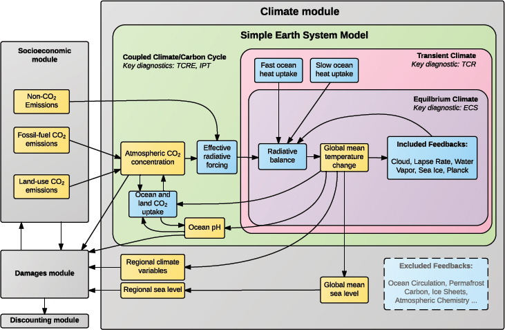
NOTES: Output variables are shown in yellow. The list of excluded feedbacks is shown. See text for discussion. See Box 4-1 for definitions of TCR, TCRE, IPT, and ECS.
using planetary energy balance to estimate global mean surface temperature changes, to Earth system models of intermediate complexity and full complexity Earth system models that project coupled changes in the atmosphere, oceans, and land surface.2 At each stage of the development of Earth system models, more comprehensive representations of feedbacks and response characteristics have been added (Flato et al., 2013), leading to increases in model resolution and the extent to which the complexity of the Earth system is represented in model structures. These representations have built on knowledge about mechanisms and relationships gleaned from increasingly comprehensive and longer-term observations of the Earth system (see, e.g., National Research Council, 2012).
Modern Earth system models represent the physics, chemistry, and biology of the atmosphere, oceans, and terrestrial hydrosphere and bio-
__________________
2 The intermediate complexity models share the structure of full complexity models, but they have a reduced set or a parameterized set of processes and feedbacks that allows faster model runs and exploration of uncertainty.
sphere at spatial and temporal scales that allow representation of their interactions and feedbacks. While energy balance models have global- or hemispheric-mean spatial resolution and annual-mean time steps, state-of-the-art Earth system models have ~100 km or finer resolution in the atmosphere and land and ~25 km resolution in the ocean with 15-minute time steps. With additional components and increasing model resolution, Earth system models capture most key elements of the scientific community’s current understanding of the complex coupled dynamical systems that govern both the Earth system’s internal variability in the absence of forcing and its response to external forcing agents.
Any SC-CO2 estimation framework has to account for uncertainty in projections of both global mean surface temperature changes and related climate variables. Computational demands of full complexity models and even of intermediate complexity models limit their ability to provide this kind of probabilistic information when very large ensembles of model runs over very long time horizons are required, as is the case with the estimates for the SC-CO2. Hence, SC-CO2 calculations require computationally efficient simple Earth system models that represent the critical behaviors captured in more comprehensive models and account for the key sources of uncertainty in climate projections. Implicitly, this also requires that such simple Earth system models are capable of reproducing key observational climate records of the past few centuries.
The next section discusses the general characteristics of a useful Earth system model, and the third section provides an overview of a simple Earth system model that satisfies these criteria. The following four sections cover key elements of that system: sea level rise; ocean acidification; spatial and temporal disaggregation, through estimating higher resolution climate variables from simple low-resolution models; and uncertainty propagation. The committee then considers some limitations of common approximations made in simple Earth system models, and the chapter concludes with a discussion of research needs.
CHARACTERISTICS OF AN ADEQUATE CLIMATE MODULE
The committee’s Phase 1 report (National Academies of Sciences, Engineering, and Medicine, 2016) suggested several criteria that could be used to evaluate whether any simple Earth model considered for use in SC-CO2 estimation reflects current scientific understanding of the relationships between CO2, other greenhouse gases, emissions, concentrations, forcing, and global mean surface temperature change, as well as their uncertainty and profiles over time. These criteria are reiterated and expanded in Recommendation 4-1.
RECOMMENDATION 4-1 In the near term, the Interagency Working Group should adopt or develop a climate module that captures the relationships between CO2 emissions, atmospheric CO2 concentrations, and global mean surface temperature change, as well as their uncertainty, and projects their profiles over time. The module should apply the overall criteria for scientific basis, uncertainty characterization, and transparency (see Recommendation 2-2 in Chapter 2). In the context of the climate module, this means:
- Scientific basis and uncertainty characterization: The module’s behavior should be consistent with the current, peer-reviewed scientific understanding of the relationships over time between CO2 emissions, atmospheric CO2 concentrations, and CO2-induced global mean surface temperature change, including their uncertainty. The module should be assessed on the basis of its response to long-term forcing trajectories (specifically, trajectories designed to assess equilibrium climate sensitivity, transient climate response and transient climate response to emissions, as well as historical and high- and low-emissions scenarios) and its response to a pulse of CO2 emissions. The assessment of the module should be formally documented.
- Transparency and simplicity: The module should strive for transparency and simplicity so that the central tendency and range of uncertainty in its behavior are readily understood, reproducible, and amenable to improvement over time through the incorporation of evolving scientific evidence.
The climate module should also meet the following additional criterion:
- Incorporation of non-CO2 forcing: The module should be formulated such that effects of non-CO2 forcing agents can be incorporated, which will allow both for more accurate reflection of baseline trajectories and for the same model to be used to assess the social cost of non-CO2 forcing agents in a manner consistent with estimates of the SC-CO2.
Comprehensive Earth system models are the scientific community’s best representations of the current understanding of the many interacting components of the Earth system. However, simple Earth system models can represent the relationship between emissions, atmospheric composi-
tion, and global mean surface temperature in a manner consistent with more comprehensive models: as shown in Box 4-1, their parameters can be set to reproduce the behavior of more complex models under a range of relevant forcing scenarios. Such consistency can be evaluated using a number of coordinated benchmark experiments that have been performed with Earth system models: in the next section, several that are particularly useful in assessing simple Earth system models that are intended to be used in SC-CO2 estimation are highlighted. Performing well against these diagnostics is not a guarantee that a climate module is appropriate for all applications, so conclusions can also, where possible, be checked against direct calculations carried out with more comprehensive models.3
As defined in Box 4-1, four key metrics can describe the configuration of a simple Earth system model: equilibrium climate sensitivity (ECS), transient climate response (TCR), transient climate response to emissions (TCRE), and the initial pulse-adjustment timescale (IPT). In addition, the overall response of the simple models to forcing can be assessed using the representative concentration pathway or extended concentration pathway (RCP/ECP)4 experiments driven by total forcing (Collins et al., 2013). The key point of comparison is whether a simple model’s central projections and projection ranges agree with those of more comprehensive Earth system models. These diagnostics would not necessarily disqualify models based on broader responses than Earth system models, which are known to cluster near central estimates (e.g., Huybers, 2010; Roe and Armour, 2011). Also, simple models can include feedbacks not represented in more comprehensive models because of more complex models’ high computational requirements, but the diagnostics could be analyzed using runs with these additional feedbacks disabled so as to facilitate comparison with more complex models that do not include such feedbacks.
__________________
3 A simple Earth system model is calibrated against more comprehensive models rather than directly against observations because there is no direct estimate of parameters such as equilibrium climate sensitivity or transient climate response because the relationship between global mean quantities in a simple model and corresponding (incompletely) observed quantities is often ambiguous (see, e.g., Richardson et al., 2016). Thus, it is generally preferred to calibrate a simple model against more comprehensive models (which have in turn been tested against observations) using idealized experiments in which, for example, only CO2 concentrations are varied.
4 Extended concentration pathways are an extension of RCP emissions scenarios from 2100 through 2300 (van Vuuren et al., 2011). See Chapter 3 for an introduction to the RCPs used in the Fifth Assessment Report of the Intergovernmental Panel on Climate Change.
BENCHMARK EXPERIMENTS FOR CALIBRATING AND EVALUATING SIMPLE EARTH SYSTEM MODELS
Temperature Response to Idealized Concentration Changes
The simplest benchmark experiments involve changing atmospheric CO2 concentrations in a (simple or complex) climate model and com-
puting the resulting global mean surface temperature response. Simple climate models,5 including those used in estimating the SC-CO2, have
__________________
5 The committee refers to “simple climate models” here rather than “simple Earth system models” to encompass models that do not have a fully interactive carbon cycle (i.e., calculating, rather than prescribing, the distribution and fluxes of carbon within the climate model.)
traditionally used ECS as a key summary indicator of the sensitivity of the climate system to changing CO2 concentrations. Since the 1990s, another widely used indicator has been TCR (see Box 4-1, above, for definitions). Successive reports of the Intergovernmental Panel on Climate Change (IPCC) have noted that ECS and TCR co-vary (Meehl et al., 2007) and that TCR is typically the more policy-relevant parameter (Frame et al., 2006; Otto et al., 2013). It is also better constrained by climate observations to date (Gregory and Forster, 2008; Libardoni and Forest, 2011, 2013). Because these quantities co-vary, varying ECS alone in any probabilistic assessment without checking the implied distribution for TCR risks introducing an implicit distribution for TCR that can be inconsistent with available observations (Meinshausen et al., 2009).
Figure 4-2 illustrates the concepts of ECS and TCR:
- Panel (a) shows global mean surface warming in idealized 1 percent per year increasing-CO2 experiments performed with the Climate Model Intercomparison Project (CMIP5) comprehensive Earth system models (black lines) compared with the Fifth Assessment Report (AR5) (see Collins et al., 2013, Figure 12.45f) assessed range for TCR (red vertical bar) and the response of a simple Earth model system (blue plume).
- Panel (b) shows warming following an instantaneous quadrupling of atmospheric CO2 concentrations in CMIP5, clearly showing a two-timescale response, with expected equilibrium warming based on assessed range for ECS (red vertical bar) and response of a simple Earth model system (blue plume).
- Panel (c) shows atmospheric concentrations in CMIP5 1 percent per year increasing-CO2 experiments plotted against cumulative CO2 emissions, compared with the historical observed airborne fraction (cumulative emissions and increase in atmospheric concentrations over the 1870-2011 period—diamond, with dashed line showing extrapolation), showing the consistent increase in airborne fraction with warming and cumulative emissions in complex Earth system models.
- Panel (d) shows temperatures in CMIP5 1 percent per year increasing-CO2 experiments plotted against cumulative CO2 emissions, showing the straight-line relationship characterized by the TCRE.
__________________
The discussion of ECS and TCR would pertain to a model driven entirely by an endogenous forcing pathway (see the boxes labeled “Equilibrium Climate” and “Transient Climate” in Figure 4-1).
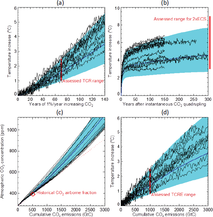
NOTES: Panel (a) shows the response to an idealized 1 percent per year CO2 increase sustained for 140 years (to quadrupling) of the CMIP5 ensemble of comprehensive climate models (black lines) and of the FAIR model (see text), with the IPCC AR5 assessed range for TCR (1-2.5 ºC).
Panel (b) shows the corresponding response to an instantaneous quadrupling of CO2 concentrations. For comparison, the IPCC’s assessed range for ECS (1.5-4.5 ºC) is shown, increased by a factor of two to correspond to a CO2 quadrupling.
Panel (c) shows the relationship between diagnosed cumulative CO2 emissions in the 1 percent per year runs and atmospheric CO2 concentration, with the convex shape indicating an increasing airborne fraction over time.
Panel (d) panel shows diagnosed cumulative CO2 emissions against warming, showing the approximate straight-line relationship discussed in the text.
The black lines reflect the results of comprehensive Earth system models. The blue plumes represent results from a simple Earth system model. See text for discussion.
SOURCE: Adapted from Collins et al. (2013, Figure 12.45f) and data from the. Coupled Model Intercomparison Project, CMIP5.
The solid black lines in panel (a) show the response of global mean surface air temperature in the CMIP5 Earth system models to a 1 percent per year increasing-CO2 scenario initiated in year 1. After the initial decade or so, all models indicate an approximately straight-line increase in temperature with time, with superimposed fluctuations due to internal climate variability.
The black lines in panel (b) show the response to an instantaneous quadrupling of atmospheric CO2 concentrations in year 1. Almost all models show a rapid initial adjustment over a decade or two, followed by a gradual warming that continues over many centuries as the global oceans slowly come into equilibrium with this new radiative forcing. Both timescales are relevant to the calculation of the SC-CO2, with the initial adjustment timescale being primarily relevant at high discount rates and the slow longer adjustment timescale relevant at low discount rates.
The red vertical bars in panels (a) and (b) show “likely”6 ranges of uncertainty for the transient climate response and the equilibrium climate sensitivity as assessed by IPCC AR5. In panel (b), the limits of the 1.5-4.5 °C assessed range for equilibrium climate sensitivity are doubled to 3-9 °C to allow direct comparison with the response of Earth system models to a quadrupling of CO2 concentrations.7 As expected, the CMIP5 model range in year 70 of these integrations (see Figure 4.2a) coincides closely with the assessed likely range for TCR. In contrast, the complex models are still far from spanning the assessed range of uncertainty in ECS even after 300 years of integration. By definition, ECS represents the warming of the climate system after it has been allowed an infinitely long time to re-equilibrate with a constant atmospheric composition, and this equilibration takes centuries to millennia in the current generation of Earth system models.
Since atmospheric composition is not expected to be constant over these timescales under any emission scenario, ECS is less directly relevant to the climate system response on policy-relevant timescales. Its prominence is to some extent a historical artefact, in that it was the aspect of the climate response that could be assessed with the “slab-ocean” climate models of the late 1970s and 1980s (e.g., Manabe and Wetherald, 1975, 1980; National Academy of Sciences, 1979; Manabe and Stouffer, 1980).
__________________
6 Likely,” in IPCC terminology (Mastrandrea et al., 2010) and as used here, means that the true value has a 66 percent or higher probability of being within the quoted range. “Very likely” means the true value has a 90 percent or higher probability of being within the quoted range.
7 Although ECS is defined as the response to a CO2 doubling, it can be evaluated against any increase, allowing for the logarithmic relationship between the change in CO2 concentration and the temperature response: in the CMIP5 model intercomparison, ECS was evaluated using a CO2 quadrupling.
TCR is most relevant to the calculation of the SC-CO2 for high values of the discount rate that emphasize the decadal response, while ECS is more important at very low discount rates in which integrated damages are dominated by the multi-century response.
The blue shaded plumes show the response of a simple Earth model system (discussed below) with low, best-estimate, and high values for TCR (panel a) and ECS (panel b). The model is consistent with the more complex Earth system models in that it reproduces key features of the model’s responses, including the linear warming after the initial decade in panel (a) and the short and long timescales of response in panel (b). Therefore, any simple climate model would have to support at least two response timescales (Held et al., 2010; Caldeira and Myhrvold, 2013; Geoffroy et al., 2013).
The ranges of uncertainty (shaded plumes) are matched to the IPCC’s assessed ranges for ECS and TCR shown by the red bars: they have not been explicitly fitted to the Earth system models, and indeed appear biased slightly low relative to the distribution of the models’ results. This is because the IPCC-assessed ranges of uncertainty in these climate system properties are based on a number of lines of evidence in addition to these climate model results—including evaluation of recent climate change and radiative forcin110g, the recent global energy budget, and paleoclimate observations—so an exact correspondence would not be expected. Emergent properties of the climate system like TCR or ECS cannot be observed directly, so all efforts to constrain them rely on some combination of observations and (simple or complex) climate modeling, and the IPCC combines multiple approaches to provide a single assessment that is consequently more robust than any estimate based on a single study.
Relationship between Emissions and Concentrations
Since the mid-2000s, many Earth system models have incorporated interactive carbon cycles, and these idealized experiments have been extended to diagnose the emissions required to increase CO2 concentrations at a prescribed rate, in addition to the uptake of CO2 by land and ocean and the residual “airborne fraction.” Panel (c) in Figure 4-2 shows atmospheric concentration of CO2 in the idealized experiments shown in panel (a) plotted against cumulative diagnosed CO2 emissions, which are the total amount of CO2 that would need to be emitted into these models to achieve the prescribed increase in CO2 concentrations, accounting for uptake by the land and oceans in the model’s carbon cycle. The slope of these lines indicates the airborne fraction: an increase of 1 ppm in concentrations for every 2.12 gigatons of carbon (GtC) (7.77 gigatons of
CO2 [Gt CO2])8 of emissions would indicate an airborne fraction of unity, meaning all CO2 emitted remains in the atmosphere. Airborne fraction in the CMIP5 models (black lines) is initially about 45 percent, similar to that observed over the historical period (dashed line and diamond), but increases as the climates warm and CO2 accumulates, due to the weakening of land and ocean carbon sinks (Jones et al., 2013). The lines are clearly convex (curving upwards), with the convexity accurately reproduced by the simple climate model (blue plume) discussed below.
The coupled climate carbon cycle response to emissions can be summarized in a plot of global mean surface temperature change against diagnosed cumulative CO2 emissions from the comprehensive Earth system models included in CMIP5 under the 1 percent per year increasing-CO2 scenario (Figure 4-2, Panel a). Despite the diversity of the CMIP5 models, the results show a linear relationship between long-term warming and cumulative CO2 emissions for cumulative emissions up to about 2,000 GtC (7,333 Gt CO2) (Gillett et al., 2013). More recent experiments show this approximate linearity holds in some models for cumulative emissions up to 5,000 GtC (18,333 Gt CO2) (Tokarska et al., 2016). This approximate linearity arises from a cancellation between the rising airborne fraction and the concave (logarithmic) relationship between CO2 concentrations and forcing. The slope of the temperature/cumulative emissions relationship is called TCRE.
Human-induced warming to date is consistent with this straight-line relationship between cumulative CO2 emissions and CO2-induced warming. However, the signal-to-noise ratio is low enough that it would also be consistent with other functional forms. Hence, it is difficult to predict the consequences of future emissions based simply on extrapolating a purely empirical approach. The two effects that give rise to this straight-line relationship in more complex models are both well supported by observations and theory. Reproducing the relationship, therefore, represents a minimum requirement for a simple Earth system model. It is not sufficient in itself, particularly in a model that is used to represent the response to both CO2 and other forcings: hence the need to check the temperature response of the model to idealized concentration changes (Panels (a) and (b)) and the airborne fraction (Panel (c)). More specific experiments can also be used to ensure that a simple model is reproducing the behavior of more complex Earth system models for the correct reasons. For example, in Gregory et al. (2009) and Arora et al. (2013), warming is artificially suppressed while CO2 concentrations increase at 1 percent per year and emissions are diagnosed as before. This allows the biogeochemistry-induced increase in the airborne fraction to be separated from the climate-induced
__________________
8 Each 1 ton of CO2 contains 0.273 tons of carbon.
increase. Verifying that a simple climate model can reproduce the relationship between cumulative emissions and concentrations under such an idealized scenario is an additional test that the changing airborne fraction (Panel (c)) is occurring for realistic reasons (Millar et al., 2016).
The spread of TCRE among Earth system models emanates from the varying sensitivities of land and ocean carbon processes to climate change, and their subsequent impact on atmospheric CO2 concentrations and climate (Arora et al., 2013). As a result of competition between CO2sensitive photosynthesis uptake and temperature-sensitive respiratory release, there is little agreement about the sign or magnitude of carbon-climate feedbacks on land uptake at the end of the 21st century. The spread among Earth system models in shifts in precipitation location, amounts, and timing further compounds this uncertainty.
For the AR5 (Ciais et al., 2013), CMIP5 Earth system models with interactive land and ocean carbon cycles coupled to the physical climate system were used to infer the emissions that would be compatible with historical and representative concentration pathway (RCP) trajectories of CO2 concentration. The uncertainty in land uptake propagates to a wide range for the “compatible” cumulative fossil fuel emissions for 2012-2100: 140-410 GtC (513-1503 Gt CO2) for RCP 2.6 and 1415-1910 GtC (5188-7003 Gt CO2) for RCP 8.5. Ocean uptake is more consistent than land uptake across Earth system models; however, scientific understanding of the biological carbon pump, especially in an acidifying ocean, remains rudimentary. Research into the responses of the land and carbon cycles and their changing capacities to absorb and store carbon is much needed. Much of the experimental and field research undertaken thus far has focused on the responses of the marine biota to increasing CO2 and temperatures. To be useful for estimating SC-CO2, the experimental design could include decreasing CO2 and constant temperature, as may occur with a pulse release (Joos et al., 2013).
Response to a Pulse Injection of CO2
Since the SC-CO2 is defined in terms of the impact of a pulse injection of CO2 into the atmosphere, one highly relevant test of the performance of a simple Earth model system is to compare its response to a pulse injection with that of more comprehensive models. This comparison is complicated by the strong dependence of the pulse response on the reference trajectory and the lack of any coordinated intercomparisons of comprehensive models focusing specifically on the pulse response to a standardized set of CO2 and non-CO2 forcings. The most comprehensive intercomparison study to date is that of Joos and colleagues (2013), in which a collection of Earth system models, Earth system models of intermediate complexity,
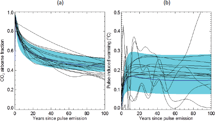
NOTES: The figure includes a range of full-complexity Earth system models, Earth system models of intermediate complexity, and simple Earth system models (black thin lines). Dark blue thick line and blue shaded region represent the median and range and mean of the response of the simple coupled climate carbon cycle model. See text for discussion.
SOURCE: Data from Joos et al. (2013) and the Coupled Model Intercomparison Project, CMIP5.
and simple Earth system models were driven with observed CO2 concentrations and non-CO2 forcing to 2010, and concentrations and forcing held constant thereafter. CO2 emissions were then diagnosed and the models were then re-run twice, once with the diagnosed emissions and a second time with a 100 GtC (367 Gt CO2) pulse of CO2 injected instantaneously in 2015. The difference between these latter two simulations provides a measure of the response to a CO2 pulse.
The temperature response following a pulse injection, shown in Figure 4-3, indicates the initial pulse-adjustment timescale (IPT), which is a measure of the timescale over which temperatures converge to their peak value in response to the pulse.9 The IPT is less than a decade in most
__________________
9 Most precisely, the IPT is the timescale over which the gap between the realized temperature and the peak temperature decays to 1/e (~37%) of its size at the time of the pulse (i.e., the exponential decay timescale).
Earth system models, meaning that peak temperatures are reached in less than two decades. This timescale is particularly important for SC-CO2 calculations at high discount rates because it determines how rapidly an injection of CO2 generates impacts. The suite of models show that peak temperatures are maintained for the duration of the model integrations, ~1,000 years, at which time about a quarter of the CO2 pulse remains in the atmosphere. As atmospheric CO2 concentrations decrease, deep ocean temperatures adjust toward equilibrium at a similar rate (Solomon et al., 2009), stabilizing surface temperatures.
This standard “impulse-response” experiment of Joos and colleagues (2013) has the advantage that many different modeling centers have performed an identical experiment. It highlights that the models converge on the deep ocean being the larger repository of the added CO2 on millennial timescales. In the first 100 years after a pulse release, large uncertainties are associated with the sink estimations, especially those of the land, echoing the CMIP5 model results where the sensitivities of land uptake to CO2 and temperature have much greater spread among the models than those of ocean uptake (Arora et al., 2013; Ciais et al., 2013). These uncertainties propagate to atmospheric CO2 concentration and the temperature response. The impulse-response experiment has the disadvantage, however, that holding CO2 concentrations constant from 2010 means that the 100 GtC pulse is introduced into an artificial “baseline” scenario of rapidly falling emissions. More realistic impulse-response experiments with comprehensive models and research into the capacities of the land and oceans to store carbon with changing climate and emissions are discussed in the conclusions of this chapter.
Response to Historical Forcings and Future Scenarios
Another test of a simple Earth model system is to compare its behavior with that of more comprehensive models when driven with observed emissions and radiative forcing over the historical period followed by a range of future forcing scenarios, such as the RCPs (Van Vuuren et al., 2011). The four RCPs are labeled RCP 2.6, RCP 4.5, RCP 6.0, and RCP 8.5, based on their respective forcing agents (in W/m2) from long-lived greenhouse gases in 2100: see Figure 4-4.
Reproducing the relationship among CO2 emissions, atmospheric concentrations, and temperatures under these scenarios of differing realistic rates and magnitudes of climate forcing can be considered as a final check rather than a means of tuning parameters in a simple Earth system model, because the multiplicity of different factors contributing to realistic historical or scenario experiments means that a simple model can reproduce the behavior of a more complex model, or the real world, for
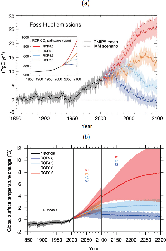
NOTES: Panel (a) shows the emissions, the inset shows the concentrations, which also include the response to land-use change emissions, and the right panel shows the temperature response to all human-induced climate forcing, including other greenhouse gases and aerosols. Panel (b) also shows response to extended scenarios for 2100-2300, showing long-term warming commitment.
SOURCE: Collins et al. (2013, Figure 12.5) and Ciais et al. (2013, Figure 6.25).
unrealistic reasons. The idealized experiments described above provide clearer information on a model’s response to CO2.
Numerical Distributions of Key Metrics
Periodic assessments of the literature regarding ECS, TCR, and TCRE are provided by the IPCC and can be used by the IWG. The most justifiable estimates of the probability distribution of these metrics will draw on a broad body of scientific research, and the IPCC provides a capable forum for conducting such assessments. In between IPCC assessments (which occur approximately every 7 years), it is likely that new results will be published indicating values that lie both at the high and the low end of IPCC assessed values. For example, the AR5 gave a “likely” range of 1.0-2.5 °C for TCR, based on 5-95 percent ranges from a number of different studies, while Shindell (2014) suggests that a TCR value less than 1.3 °C is “very unlikely,” and Richardson and colleagues (2016) suggest an upward revision in the upper bound. Conversely, Lewis and Curry (2014), while finding a 5-95 percent range in agreement with the AR5 range, argue for a best-estimate value toward the lower end. As Richardson and colleagues (2016) demonstrate, the precise numbers can be sensitive to the choice of observations used, the assumptions underlying the analysis method, and even the definition of global average surface temperature. On a more subtle level, it has long been known (Frame et al., 2005) that statistical prior assumptions can affect the modes of an estimated statistical distribution of an indirectly observed climate parameter in ways that may not be transparent to a user. Reliance on any individual study therefore risks introducing volatility into SC-CO2 estimates; it can be avoided by relying on the IPCC’s more comprehensive periodic assessments based on multiple lines of evidence.
The AR5 provided formally assessed uncertainty ranges for ECS, TCR, and TCRE, although it does not specify either distributional forms or joint distributions. The AR5 also does not provide formally assessed ranges for other climate metrics that are relevant to the SC-CO2 estimates, including IPT, the TCR/ECS ratio (also known as the realized warming fraction, [RWF]), and the expected increase in CO2 airborne fraction between the 20th and 21st centuries (although this latter quantity is, to some degree, implicit in TCRE). Hence, although much of the information on the climate system response required by the IWG is contained in the IPCC assessments themselves, it would likely be necessary to consult relevant experts (including the responsible IPCC authors and reviewers) to ensure this information is used consistently. There is also an opportunity for the IWG to inform future IPCC assessments by highlighting important policy-relevant metrics on which specific guidance is requested.
The assessed IPCC likely range for ECS is 1.5-4.5 °C, while the assessed likely range for TCR is 1.0-2.5 °C. In the coupled models of the CMIP5 ensemble, ECS and TCR are strongly correlated, but TCR and the RWF are nearly uncorrelated (Millar et al., 2015). A convenient way of capturing the correlation between ECS and TCR is thus to specify TCR and RWF as a joint distribution of two statistically independent parameters; a likely range of 0.45-0.75 for RWF is consistent with the AR5 ranges for TCR and ECS. For TCRE, AR5 estimates a likely global warming of 0.8-2.5 °C per 1000 GtC cumulative emission for cumulative emissions less than 2000 GtC; subsequent studies (Tokarska et al., 2016) suggest the linearity may extend to a higher range, while others have found that it may not (Herrington and Zickfeld, 2014).
Although these ranges are referred to as “likely” by the IPCC, they are closer to 90 percent confidence intervals in the majority of supporting studies, and they also encompass about 90 percent of model responses in the CMIP5 ensemble. The reason for the IPCC’s more conservative likelihood qualifier is that structural uncertainties, common to all studies and models, may affect conclusions. In general, there are two ways of dealing with structural uncertainty: it can be parameterized by including an additional error term, or quantitative results can be computed ignoring structural uncertainty and conclusions subsequently qualified to account for that omission. The IPCC takes the second approach, recognizing that any quantitative representation of structural uncertainties that are common to all studies and models would be difficult to justify. This is illustrated, for example, in Figure 4-5a. Consistent with the IPCC’s supporting studies, 90 percent of ECS/TCR values lie in the 1.5-4.5/1.0-2.5 °C interval, so to be consistent with the IPCC’s interpretation, 90 percent ranges of the outputs in the other three panels ought to be interpreted as “likely” ranges of uncertainty.
Thus, a number of methods exist to translate uncertainty ranges assessed by the IPCC into probability distributions. In the interest of transparency, the IWG could define explicitly the interpretation it proposes to use in consultation with relevant IPCC authors and reviewers. One possible option in Figure 4-5a is presented, while recognizing that others are defensible.
RECOMMENDATION 4-2 To the extent possible, the Interagency Working Group should use formal assessments that draw on multiple lines of evidence and a broad body of scientific work, such as the assessment reports of the Intergovernmental Panel on Climate Change, which provide the most reliable estimates of the ranges of key metrics of climate system behavior. If such assessments are not available, the IWG should
derive estimates from a review of the peer-reviewed literature, with care taken so as to not introduce inconsistencies with the formally assessed parameters. The assessments should provide ranges with associated likelihood statements and specify complete probability distributions. If multiple interpretations are possible, the selected approach should be clearly described and justified.
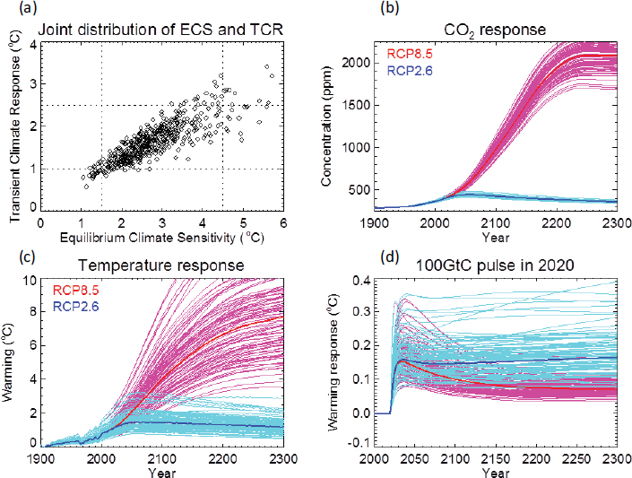
NOTE: Panel (a) shows the joint distribution used for ECS and TCR. Panel (b) shows CO2 concentrations in response to prescribed emissions associated with RCP 2.6 (blue) and RCP 8.5 (red/pink). Panel (c) shows temperature response to RCP 2.6 and RCP 8.5. Panel (d) shows temperature response to a pulse emission of 100 GtC released in 2020 into a background RCP 2.6 (blue) and RCP 8.5 (red/ pink) scenario.
SOURCE: Adapted from Millar et al. (2016).
Transparency and Simplicity
The basic physics of the equilibrium global mean temperature response to radiative forcing has been understood since the late 19th century. More recent work has shown that the dynamics of the global mean temperature response to forcing and to emissions in complex climate models can be reproduced by simple approximations. Simple models bring great benefits in terms of both transparency and the ease with which they can be used in a probabilistic mode; thus, it makes sense for SC-IAMs10 to use Earth system models that are as simple as possible while accurately capturing key behaviors of the climate system. Models that can be readily reproduced from a minimal set of well-documented equations are particularly useful. An example of good practice is the model provided for the calculation of greenhouse gas metrics, which is fully documented in the Supplementary Online Material of Chapter 8 of the AR5 (Myhre et al., 2013) and provides the basis for the Finite Amplitude Impulse Response (FAIR) model, detailed below.
Incorporation of non-CO2 Forcing Agents
CO2 is not the only important climate forcing agent; other key agents include methane, nitrogen oxides, fluorinated gases, and aerosols. To accurately estimate the response of the climate system to a pulse release of CO2, any Earth system model needs to include the effects of these other agents as well, as the response depends nonlinearly on climate itself. This approach also allows the same modeling framework to be used for the calculation of the social cost of climate forcing agents other than CO2. Non-CO2 greenhouse gases generally exhibit simpler biogeochemical cycles than CO2, and their atmospheric concentrations can be reasonably well approximated by a simple exponential decay (Myhre et al., 2013).
Aerosols are short lived in the atmosphere. While their global average climate forcing can be crudely approximated as proportional to total emissions, different spatial patterns of emissions give rise to significantly different spatial patterns of temperature change. These spatial patterns cannot be directly modeled in a simple Earth system model (see discussion of disaggregation below), so an approximation of effective forcing as proportional to emissions is reasonable, but it introduces ambiguity in the interpretation of global average aerosol forcing in the context of simple models. This ambiguity is one of the key reasons that attempting to calibrate a simple Earth system model’s properties against historical
__________________
10 These are the three integrated assessment models widely used to produce estimates of the SC-CO2 (see Chapter 1).
observations using simple energy-balance models is problematic (e.g., Shindell, 2014).
AN ILLUSTRATIVE SIMPLE EARTH SYSTEM MODEL: OVERVIEW
As an example of a simple Earth system model that satisfies the criteria set forth above, the committee considered the FAIR model (Millar et al., 2016). FAIR is a minor modification of the model used in the AR5 to assess the global warming potential of different gases (Myhre et al., 2013), which the committee will call the Static Impulse Response (SIR) model. FAIR is extended with a state-dependent carbon uptake to incorporate feedbacks between the climate and the carbon cycle and thus reproduce the CO2 behavior of more complex models, in particular the changing airborne fraction with rising temperature and cumulative emissions, which is shown in Figure 4-2c (above).
In the Earth system, the rate of CO2 loss from the atmosphere is governed by exchange with the ocean, the terrestrial biosphere, and, ultimately, geological reservoirs. To represent this as simply as possible, FAIR divides the excess atmospheric CO2 concentration above the preindustrial baseline value, C0, into four fractions, denoted Ri, all of which are empty in preindustrial equilibrium. Each emission of CO2 is partitioned between the fractions in proportions specified by ai, and each fraction has its own loss time constant, τi. A single state-dependent scaling factor, α, modulates the four time constants and is defined in equation (4). CO2 concentrations in the four fractions are updated thus:
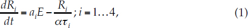
where E is the CO2 emissions rate, expressed for convenience in terms of atmospheric parts per million per year (1 ppm = 2.12 Gt C = 7.77 Gt CO2). This is mathematically equivalent to modeling the carbon cycle with four reservoirs of different capacities between which carbon is allowed to flow at different rates, although the Ri in equation (1) refer to fractions of excess CO2 in the atmosphere (i.e., above preindustrial levels) that are responding on different timescales, and do not correspond to actual quantities in different biogeochemical reservoirs.
Atmospheric CO2 concentrations are given by adding concentrations in the different fractions to preindustrial concentrations, C = C0 + ∑iRi, and radiative forcing, F, by:
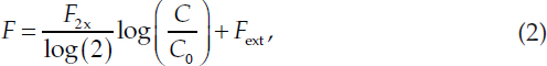
where F2x is the forcing due to a CO2 doubling, and Fext is the non-CO2 forcing.
For the energy balance component, FAIR estimates the temperature, Ti, for two ocean layers (i.e., thermal reservoirs) that have slow and fast response timescales (d1 and d2). Thus:
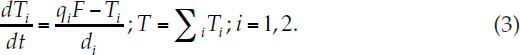
The parameters q1 and q2 can be set to give any desired combination of ECS and TCR: ECS ![]() TCR
TCR ![]() where bi represents the fraction of the equilibrium warming of the ith response component that is manifest after a 70-year linear forcing increase, bi = 1 – di (1 – exp(–70/di))/70 (as described in Millar et al., 2015). The shorter of the two thermal adjustment times, d2, largely determines the IPT (see below for representative values).
where bi represents the fraction of the equilibrium warming of the ith response component that is manifest after a 70-year linear forcing increase, bi = 1 – di (1 – exp(–70/di))/70 (as described in Millar et al., 2015). The shorter of the two thermal adjustment times, d2, largely determines the IPT (see below for representative values).
The sole structural difference between FAIR and the static impulse response model is the introduction of the state-dependent coefficient a. A suitable state-dependence for a can be determined from its relationship with the 100-year integrated impulse response function, iIRF100, discussed in Joos et al. (2013), which is the integral of the concentration response over the century to a unit pulse emission of CO2:
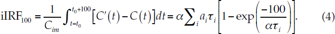
In this equation, C’(t) represents the CO2 concentration at time t following the emission pulse, Cim, added at time t0, and C(t) the CO2 concentration without the pulse. FAIR assumes that iIRF100 is a simple linear function of accumulated perturbation carbon stock in the land and ocean, which is the difference between cumulative emissions to date (“reference” emissions plus pulse) and the excess carbon in the atmosphere (i.e. neglecting geological uptake on these timescales), ![]() and of global temperature departure from preindustrial conditions, T:
and of global temperature departure from preindustrial conditions, T:
![]()
FAIR is integrated by computing iIRF100 at each time-step using Cp and T from the previous time-step using equation (5), computing ![]() using equation (4) and applying it to the carbon cycle equations (1). Hence, the iIRF100 is only exactly reproduced under constant background conditions with infinitesimal perturbations. Values of r0 = 35 years, rC = 0.02 years/GtC and rT = 4.5 years per degree Celsius (°C), with other parameters as given in the supplementary online material of Myhre and colleagues (2013), together with ECS = 2.7 °C and TCR = 1.6 °C, give a
using equation (4) and applying it to the carbon cycle equations (1). Hence, the iIRF100 is only exactly reproduced under constant background conditions with infinitesimal perturbations. Values of r0 = 35 years, rC = 0.02 years/GtC and rT = 4.5 years per degree Celsius (°C), with other parameters as given in the supplementary online material of Myhre and colleagues (2013), together with ECS = 2.7 °C and TCR = 1.6 °C, give a
numerically computed iIRF100 of 53 years for a 100 GtC pulse released against a background CO2 concentration of 389 ppm following a historical build-up. This value is consistent with the central estimate of Joos and colleagues (2013).
As noted above, the IPCC does not provide explicit distributions of ECS and TCR. Most supporting studies indicate positively skewed distributions, although not in most cases as heavily skewed as that of Roe and Baker (2007). Pueyo (2012) argues that for scaling parameters like ECS and TCR—positive quantities in which the larger the parameter, the greater the uncertainty—a log-normal distribution might be appropriate. Noting that the “likely” ranges quoted by the IPCC correspond to 5-95 percent ranges in the supporting studies, assuming a log-normal distribution for TCR with a 5-95 percent range of 1.0-2.5 oC, together with a normal distribution for RWF with a 5-95 percent range of 0.45-0.75, gives a joint distribution of ECS and TCR that is consistent with the distribution of more complex Earth system models.
Reproducing a distribution for TCRE requires accounting for the additional uncertainties in the carbon cycle. The AR5 does not provide assessed uncertainty ranges in carbon cycle properties, but varying iIRF100 by ±7 years (5-95% range) gives a distribution of CO2 concentration trajectories consistent with uncertainties of past emissions and concentrations (shown in Figure 4-2c, above). It also provides a 5-95 percent range for TCRE derived from 1 percent per year increasing-CO2 experiments of 0.8-2.6 °C/TtC (Figure 4-2d, above), in close agreement with the AR5 assessed “likely” range. This plot of CO2-induced warming against cumulative CO2 emissions is very similar to the corresponding plot derived from more complex models (see Intergovernmental Panel on Climate Change, 2013, Figure 10), in that it is almost straight and slightly concave at high values. A simple climate model that omits carbon cycle uncertainty represented in the state-dependent iIRF100 would necessarily display a very different shape, strongly concave over the full range.
Finally, the key parameter determining the IPT is the short thermal adjustment time, d2. The IPCC does not give an assessed range for IPT, so a median value of 4.1 years with a 5-95 percent range of 2-7 years, based on the range of behavior of the CMIP5 models (Geoffroy et al., 2013), is used for illustration here. Results are generally insensitive to the specification of the longer timescale, d1. For consistency, and in the absence of an assessed range for this parameter, the committee also uses the multimodel mean estimate from Geoffroy and colleagues (2013) of 229 years. Blue lines in Figure 4-5b shows the response of the global mean temperature to a pulse injection of 100 GtC of CO2 in 2020 against a background ambitious mitigation (RCP 2.6) scenario. The overall behavior is very consistent: a rapid adjustment on a timescale of the order of a decade or less to
a temperature plateau that persists for a century or more. The red/pink lines show the corresponding result against a background no-mitigation (RCP 8.5) scenario: the rapidly rising background warming results in a declining response to the input pulse.
As a proof of concept, FAIR provides an example of a model consistent with all three of the criteria in Recommendation 4-1 (above). First, its parameters can be set so as to yield distributions of ECS, TCR, TCRE, IPT, and responses to RCP pathways consistent with the responses of more complex earth system models, as illustrated in Figures 4-2 and 4-5 (above). Second, it is simple and transparent. Third, non-CO2 radiative forcing can be straightforwardly introduced through the Fext term, and because the model is structurally identical to that used by the IPCC for lifetime and metric calculations for a broad range of greenhouse gases, it can readily be applied to compute the response to, for example, methane and nitrous oxide emissions with a simple change of values of the parameters ai and ti. Note that, for gases whose behavior can be characterized by a single exponential decay life-time, three of the ai can be set to zero.
Each element of FAIR is necessary to allow ECS, TCR, TCRE, and IPT to be set independently and to demonstrate relevant behaviors seen in higher complexity models. Consistent with equation (3) (above), the climate system exhibits two dominant timescales of response to forcing, reflecting the response of the mixed layer and the deep ocean (Hansen et al., 1984; Gregory, 2000; Held et al., 2010; Geoffroy et al., 2013). Consistent with equation (1) (above), four timescales are necessary to describe the uptake of CO2 by the land biosphere, surface ocean, deep ocean, and geological reservoirs (Joos et al., 2013).
The feedback between the climate and the carbon cycle represented by the scaling factor, a in equations (1) and (4), is necessary to yield a near-linear relationship between cumulative emissions and warming; if a is fixed to equal 1, as in the static impulse response model, this behavior cannot be reproduced (Millar et al., 2016). Similarly, this feedback is necessary to show the increase in airborne fraction needed to jointly reproduce, with a single set of model parameters, both 20th- and 21st-century behavior seen in the CMIP5 Earth system models (see Figure 4-2 above).
The comparison of the FAIR model to the benchmark experiments described above are shown in Figures 4-2 and 4-5 (above), using a representative distribution of parameters: note how both comprehensive Earth system models and the simple Earth system models show a rapid initial adjustment (short IPT) to a pulse emission in 2020. The FAIR model shows an approximately constant temperature response over the first few centuries, although its millennial timescale behavior appears to underestimate the persistence of the warming. This illustrates the importance of using such comparisons to identify aspects of simple model behaviors that
are particularly relevant to the SC-CO2 estimation: whether the model response beyond 300 years is relevant would depend on the discount rate and damage function, among other factors.
Comparing the minimal simple FAIR model described above to the simple Earth system models in the existing SC-IAMs (see Appendix E), the committee finds that each of the SC-IAM models omits at least one key element. Specifically, all SC-IAMs omit the short adjustment timescale of the thermal response (although the Dynamic Integrated Climate-Economy [DICE] supports two response timescales, as implemented, both are multidecadal or longer). DICE also omits the feedback from climate change to the carbon cycle, which would impact its long-term response, and the short carbon cycle adjustment timescale, which would impact its IPT. The Framework for Uncertainty, Negotiation and Distribution (FUND) and Policy Analysis of the Greenhouse Effect (PAGE) models both represent the thermal response with a single (multidecadal) timescale only. Carbon cycle feedbacks are represented in FUND and PAGE, but it would require further research to establish whether these representations are structurally equivalent to FAIR. With these exceptions, the model components of DICE, FUND, and PAGE are structurally equivalent to special cases of the FAIR model described above, and hence they could be modified to satisfy the criteria outlined in Recommendation 4-1 (above) and the requirements in Conclusion 4-1. Furthermore, differences in the implementation of the models that are affecting results could also be addressed.
CONCLUSION 4-1 The simplest possible model capable of (a) flexibly representing equilibrium climate sensitivity (ECS), transient climate response (TCR), and transient climate response to emissions (TCRE), and initial pulse adjustment timescale (IPT) and (b) incorporating responses to forcing agents other than CO2 requires:
- two timescales, one subdecadal, the other centennial, of the surface temperature and ocean heat content response to radiative forcing;
- at least three distinct timescales of the atmospheric CO2 response to emissions, corresponding to atmospheric exchanges with the land and surface ocean, the deep ocean, and geological reservoirs; and
- a state-dependent carbon cycle in which the fraction of emitted CO2 that remains in the atmosphere increases in response to higher temperatures and accumulation of carbon in the land and ocean.
PROJECTING SEA LEVEL RISE
Global mean sea level (GMSL) rise is one of the key physical parameters relevant for estimating climate damages. GMSL rise results from both the transfer of water mass from continental ice sheets and glaciers into the ocean and the volumetric expansion of ocean water as it warms. Historically, direct anthropogenic transfer of water between the continents and the oceans, through groundwater depletion and the construction of dams, has been a tertiary contributor to GMSL change (Church et al., 2013).
In principle, heat uptake in a model like FAIR could be used to diagnose the contribution of thermal expansion to global mean sea level rise. However, as noted by the AR5, thermal expansion accounts for less than half of both historical and projected GMSL (Church et al., 2013), so accounting only for this term would provide an incomplete estimate of GMSL rise. A variety of authors have demonstrated methods for probabilistically projecting GMSL rise, based either on bottom-up accounting of contributing factors (e.g., Jevrejeva et al., 2014; Kopp et al., 2014; Slangen et al., 2014) or on top-down, semi-empirical, statistical estimates of the relationship between global mean temperature and global mean sea level (Rahmstorf, 2007; Grinsted et al., 2009; Vermeer and Rahmstorf, 2009; Kopp et al., 2016a). Because the different contributors to GMSL change exhibit different spatial patterns (Milne et al., 2009; Kopp et al., 2015), only bottom-up accounting directly allows for projection of local sea level changes. Starting from Rahmstorf (2007), Kopp and colleagues (2016a) demonstrate a semi-empirical model, calibrated against a 2-millennia record of temperature and sea level change, that agrees well with bottom-up estimates, including those of the AR5 (Church et al., 2013; Kopp et al., 2014), while Mengel and colleagues (2016) demonstrate a semi-empirical method, calibrated against model-based estimates of different contributing factors, that yields similar results. Both examples provide suitable models for estimating GMSL rise from global mean temperature projections.
In the model from Kopp and colleagues (2016a), global mean sea level h is described by
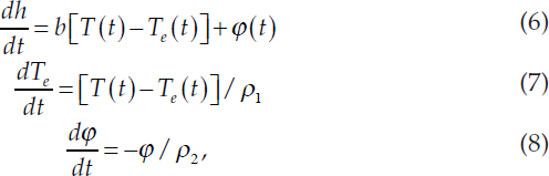
where T is global mean temperature, Te is the global mean temperature with which sea level is in quasi-equilibrium, φ is a multi-millennial scale contribution to sea level rise from Earth’s long-term climate cycles, b is a
scale factor, and ρ1 and ρ2 are timescales. Figure 4-6 shows an example of projections from this model.
However, semi-empirical models are, by construction, calibrated to the historical record over the past couple of centuries or millennia and do not reflect novel behaviors not exhibited in this record. The emerging agreement between semi-empirical models and many bottom-up models could be interpreted as suggesting that bottom-up models also exhibit a historical bias.
Indeed, DeConto and Pollard (2016) suggest that all these projections may be underestimating the 21st century Antarctic contribution to sea level rise by excluding some important physical processes involving ice shelves and ice cliffs. In contrast to the AR5’s projection of a likely –0.04 to +0.14 m contribution from Antarctica over the 21st century under RCP 8.5 (Church et al., 2013), DeConto and Pollard (2016) suggest that the physics of ice shelf hydro-fracturing and ice cliff collapse could allow contributions of 1.3 m or more. This is an emerging area of research that will require monitoring. Advances in semi-empirical models of sea level rise are qualitatively different from most new publications addressing metrics for energy balance models, such as ECS and TCR, that appear between IPCC assessments because they are incorporating physical processes that have not previously been taken into account.
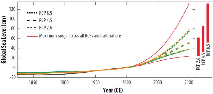
NOTES: The black curve shows the historical reconstruction of Kopp et al. (2016a), while the nearly overlapping dashed orange and green curves show median projections under three RCPs, using temperature calibrations to either Mann et al. (2009) (orange) or Marcott et al. (2013) (green). Bars show the 90 percent probability interval of projections for 2100.
SOURCE: Kopp et al. (2016a, Figure 1e-f).
CONCLUSION 4-2 Semi-empirical sea level models provide a simple and probabilistic approach to estimate the global mean sea level response to global mean temperature change and its uncertainty. However, both semi-empirical models and many more detailed models of sea level change may exhibit a bias toward historical behaviors. In particular, they may not account for some ice sheet feedbacks and threshold responses that were unimportant over the past several millennia but could become important in response to human-induced climate change. Accordingly, estimates of sea level rise and sea level–related damages, particularly beyond 2100, need to be used with the recognition that they may understate long-run sea level uncertainty in ways that are difficult to quantify.
RECOMMENDATION 4-3 In the near term, the Interagency Working Group should adopt or develop a sea level rise component in the climate module that (1) accounts for uncertainty in the translation of global mean temperature to global mean sea level rise and (2) is consistent with sea level rise projections available in the literature for similar forcing and temperature pathways. Existing semi-empirical sea level models provide one basis for doing this. In the longer term, research will be necessary to incorporate recent scientific discoveries regarding ice sheet stability in such models.
Sea level rise is not spatially uniform, so GMSL projections may need to be regionalized for use in the damages module. Bottom-up projections of regional sea level rise (e.g., Kopp et al., 2014) can be used to calibrate the relationship between global the mean sea level and regional sea level change. A reasonable approximation of these bottom-up estimates may be represented as a linear function of global mean sea level change. A better approximation can be achieved by representing local sea level as the sum of a nonclimatic, constant-rate term and a climatic component that scales with global mean sea level change, such as:
![]()
where SL indicates local relative sea level at location x and time t, k(x) a scaling coefficient, and m the rate of non-climatic processes. Figure 4-7 shows an estimate of k(x) and its uncertainty, as well as of m(x), from Kopp and colleagues (2014). The committee notes that k(x) is not identically unity due to a range of factors including ocean dynamics and the
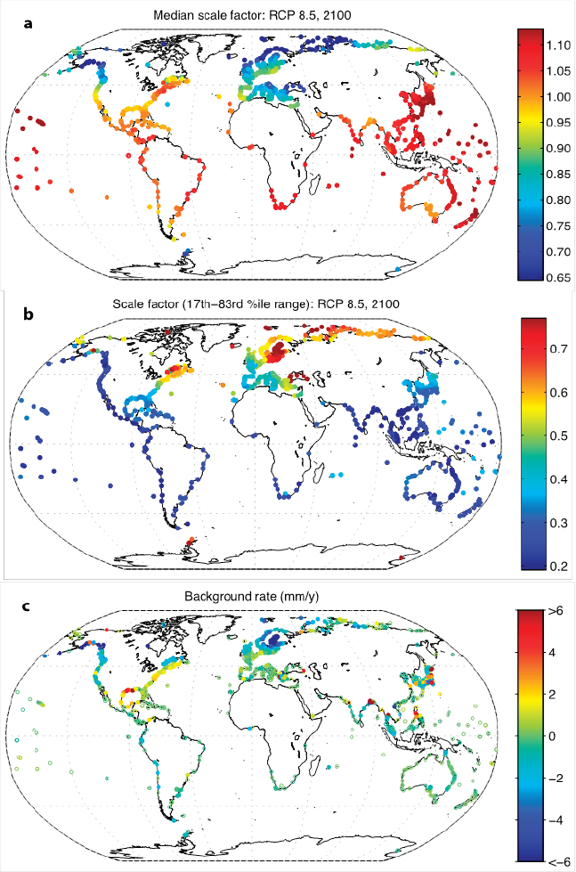
NOTE: Panel (a) Median scale factor κ(x) for the relationship between climatically driven local sea level change and global mean sea level change, panel (b) the likely (17th-83rd percentile) range of uncertainty in κ(x), and panel (c) mean estimate of the nonclimatic rate of sea level rise m(x), as estimated at a global network of tide-gauge sites.
SOURCE: Kopp et al. (2014, Figure 6).
gravitational, rotational, and land motion effects of redistributing mass between the ocean and the cryosphere (Kopp et al., 2015).
PROJECTING OCEAN ACIDIFICATION
CO2 dissolves in seawater to form carbonic acid. As the oceans have absorbed about one-quarter to one-third of the anthropogenic CO2 emissions, the oceans have steadily become more acidic, with pH decreasing by 0.02 units per decade since measurements began in 1980s (Bates, 2007; Doney et al., 2009; Dore et al., 2009). Ocean acidification has damaging consequences for many organisms, such as corals, bivalves, and mollusks that produce shells or skeletal structures out of carbonate minerals, as well as microorganisms at the base of the marine food web.11 In this way, ocean acidification can contribute to the SC-CO2 estimate through both damages to fisheries and damages to ecosystem services (Cooley and Doney, 2009; Cooley et al., 2015; Gattuso et al., 2015; Mathis et al., 2015). To the committee’s knowledge, ocean acidification is included in only one integrated assessment model (IAM) (Narita et al., 2012).
Ocean carbonate chemistry is fairly well understood, and so ocean pH can be parameterized as a function of the partial pressure of CO2 in surface waters: Figure 4-8 (see Appendix F for the derivation):
![]()
where pH = −log10[H+] is defined on the “total” hydrogen ion scale (Dickson, 1981) and pCO2 is in micro-atmospheres. Globally averaged surface ocean pCO2 lags behind globally averaged atmospheric CO2 by approximately 1 year, and so the trend in pH can be readily derived from the trend of atmospheric CO2 in simple Earth system models.
Another approach for deriving pH in simple models is as a quadratic function of concentration of dissolved inorganic carbon (DIC), with the three coefficients themselves quadratic functions of temperature (see Appendix F for the equation and its derivation). As shown in Figure 4-8 (right panel), the upper ocean becomes more acidic with increasing concentration of dissolved inorganic carbon and with increasing temperature.
__________________
11 In laboratory experiments and in limited coastal studies, some commercially important shellfish species (e.g., mussels, oysters, scallops, clams, crabs) show decreased development or shell dissolution in more acidic waters (e.g., Fabry et al., 2008; Barton et al., 2012). Juveniles are particularly sensitive to acidification, and these consequences may be exacerbated by ocean warming (see, e.g., Rodolfo-Metalpa et al., 2011). The impacts of acidification propagate through marine food webs to aquaculture and marine fisheries. Furthermore, damaged coral reefs reduce tourism, coastal protection, and biodiversity.
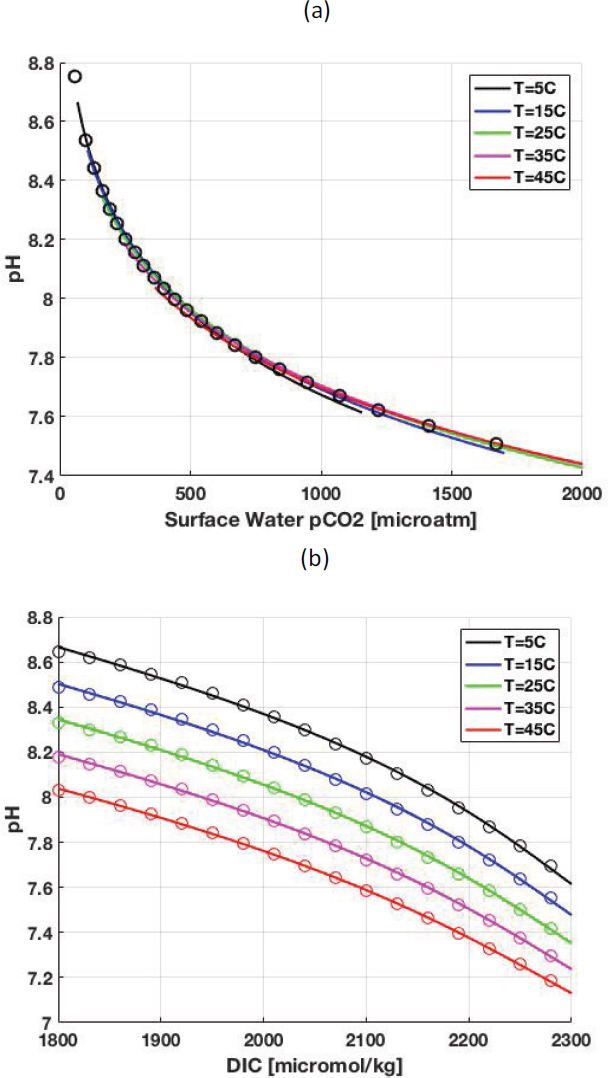
NOTES: Calculated with carbon chemistry code CO2SYS.m (solid) and with empirical equations (circles). See Appendix F for the equations and their derivation.
This approach would be the starting point for estimating regional changes in pH.
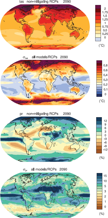
The degree of ocean acidification thus is directly related to the amount of anthropogenic CO2 taken up by the oceans as a function of time. In turn, acidification alters the relative abundance of carbonate species in surface waters and slows the ocean uptake of anthropogenic CO2. This feedback is captured implicitly in simple earth system models whose pH projections are consistent with those in earth system models where ocean carbonate chemistry and biology is included explicitly. This is illustrated with FAIR. Atmospheric CO2 fractions in the FAIR model do not represent actual amounts of carbon in any specific location. Rather they represent perturbations away from equilibrium for adjustments on a given timescale. If one assumes that the shortest (4-year) adjustment timescale for atmospheric CO2 concentrations includes uptake by the near-surface oceans, then near-surface concentration of DIC can be represented by the following formula:
where DIC0 is the unperturbed DIC concentration, R4 is the perturbation concentration in the fastest-adjusting fraction, the partition coefficients ai are as given above, and η is a proportionality constant. Following a pulse injection of CO2 into the atmosphere, the DIC anomaly in the near surface ocean initially increases from zero over about 4 years, and subsequently varies as penetration of excess carbon to the deep ocean in proportion to the atmospheric CO2 concentration anomaly. A proportionality constant of η = 0.43 converts the ocean carbon uptake from R (in ppm) to DIC (expressed in micromol/kg), typically used in ocean carbon observations.
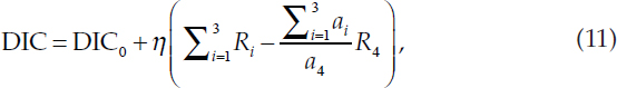
Using this relationship to convert DIC into tropical pH (assuming an initial average temperature of 25 °C and initial DIC of 2030 micromol/kg, thereby giving an initial pH of 8.15), gives a simulated pH under RCP 8.5 and RCP 2.6 that compares well with Working Group 1 of AR5 Figure 6.28: see Figure 4-9b.
The global distribution of pH is not uniform: it reflects the interaction between carbonate chemistry, biology, and ocean circulation. In general, pH is lowest, ~8.10 units, in the equatorial oceans, and increases to ~8.23 units in the Arctic Ocean (Bopp et al., 2013). CMIP5 models project globally averaged pH to decrease by 0.30-0.32 units by 2100 with the RCP 8.5 scenario, and by 0.06-0.07 units for the RCP 2.6 scenario (Ciais et al., 2013). Regional changes are projected to be greatest and fastest in the Arctic and Southern Oceans, where lower salinity (from sea ice melt and increased precipitation) and enhanced carbon uptake (from greater ice-
NOTES: Panel (a): estimated for the Arctic, Southern Ocean, and the Tropics by 11 earth system models (Ciais et al., 2013); panel (b): using Equation (11) in the text and FAIR (Millar et al., 2016).
SOURCE: For panel (a), Ciais et al. (2013, Figure 6.28).
free areas) exacerbate the effects of anthropogenic CO2 uptake (Orr et al., 2005; Steinbacjer et al., 2009; Yamamoto et al., 2012). As calcium carbonate is more soluble at cold than at warm temperatures, undersaturation of aragonite, a prevalent and more soluble form of calcium carbonate, is projected to commence in the Arctic winter around 2020 and become widespread in the Arctic and Southern Oceans when atmospheric CO2 reaches 500-600 ppm (McNeil and Matear, 2008; Steinacher et al., 2009). Coastal upwelling regions, such as the California current system, are projected to be equally vulnerable as strong seasonal upwelling brings water with higher carbon concentrations and lower pH from depth to the surface (see, e.g., Hauri et al., 2013).
Modeling of the consequences of ocean acidification on the marine biota is at an early stage, and it is mainly carried out using Earth system or regional ocean models with comparable complexity. The committee is unaware of any empirical relationship that relates regional pCO2 or DIC changes to a projection of change in globally averaged pCO2 or DIC: such relationships would be important for assessing regional damages associated with ocean acidification.
RECOMMENDATION 4-4 The Interagency Working Group should adopt or develop a surface ocean pH component within the climate module that (1) is consistent with carbon uptake in the climate module, (2) accounts for uncertainty in the translation of global mean surface temperature and carbon uptake to surface ocean pH, and (3) is consistent with observations and projections of surface ocean pH available in the current peer-reviewed literature. For example, surface ocean pH can be derived from global mean surface temperature and global cumulative carbon uptake using relationships calibrated to the results of explicit models of carbonate chemistry of the surface ocean.
SPATIAL AND TEMPORAL DISAGGREGATION
Simple climate models produce climate projections that are highly aggregated both spatially and temporally. For example, the FAIR model produces projections of climatological (multidecadal average) global mean temperatures. Yet no one lives at 30-year global mean conditions; damages are caused by the day-to-day, place-specific experiences of the weather, the statistical properties of which are described by the climate. Thus, the damages module will either require geographically and temporally disaggregated climate variables as input or such disaggregation
will need to occur in the calibration of the relationship between highly aggregated climate variables and resulting damages.
Intermediate approaches are also possible. For example, elements of the FUND and PAGE damage functions are defined with respect to climatological temperature at the spatial scale of subcontinental regions, and linear scaling relationships are used to relate global mean temperature to these regional averages. Higher-resolution climate data can be used to calibrate the relationship between regional temperature and damage. Some studies using process-based IAMs Earth system models of intermediate complexity produce latitudinal-average climate variables (e.g., Schlosser et al., 2012). Climate variables at ~1° spatial resolution and daily temporal resolution have been used to drive other studies of economic risks (e.g., Carlos et al., 2014; Houser et al., 2015; Waldhoff et al., 2015), though these have generally been bound to follow fixed scenarios (e.g., the RCPs) run with general circulation models.
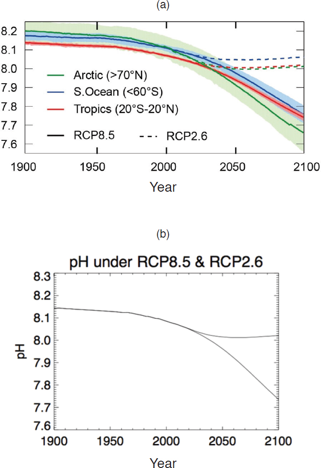
The most straightforward approach to estimate the distribution of spatially disaggregated variables conditional on global mean variables is to use data from Earth system model runs to estimate linear relationships between local climate variables (e.g., temperature, precipitation) and global mean variables (e.g., temperature). This approach is known as pattern scaling (Mitchell, 2003; Tebaldi and Arblaster, 2014). With the climate module providing global mean temperature T(t), the disaggregated regional climate variable Ds is estimated as a scaling by a fixed pattern, usually season dependent:
![]()
where s denotes the season, x the spatial location, and p the pattern: see Figure 4-10.
Pattern scaling suffers from a number of known limitations (Tebaldi and Arblaster, 2014). It performs reasonably well for regional average temperatures; it performs less well for variables, such as precipitation, that have a high ratio of natural variability to forced change and that may have a nonlinear relationship with temperature. It also performs more reliably under conditions of rising forcing than under conditions of stable or declining forcing, as the response of the Earth system to forcing evolves over time. Some variables respond significantly differently to aerosol forcing than to greenhouse gas forcing; some slightly more sophisticated pattern scaling approaches have attempted to incorporate this dependence (Frieler et al., 2012).
Pattern scaling as generally used produces projections of climatological averages, but impact models may require higher temporal resolution. More development is needed in this area. Some researchers (e.g.,
NOTES: Multimodel mean patterns (panels a and c) for annual mean surface air temperature (top panels) and precipitation (bottom panels) over the 21st century for nonmitigation pathways (RCP 4.5 and RCP 8.5), and the standard deviations (panels b and d) across both models and concentration pathways (RCP 2.6, 4.5, and 8.5). Temperature maps in units of °C regional change per °C global mean temperature change; precipitation maps in units of percent regional precipitation change per °C global mean temperature change.
SOURCE: Adapted from Tebaldi and Arblaster (2014, Figures 3 and 4).
Rasmussen et al., 2016) have attempted to address this issue by combining pattern-scaled variables with time series of residuals unexplained by the linear model:
![]()
These residuals could also be estimated by looking at the relationships in the observational record between climatological seasonal means and daily weather, and they could be more cleanly separated from the forced changes represented by T(t)ps(x) using large initial-condition ensembles of runs from individual Earth system models (e.g., Kay et al., 2014). Whether such temporal disaggregation is necessary in the context of the SC-CO2 estimation depends on how the damages module is calibrated. One approach that may be most feasible in the near term, which is similar to that currently employed by the SC-IAMs, is to make the temporal disaggregation implicit in the damages module, implying that the damages module takes as input climatological average variables.
Given the available existing archives of Earth system model results, such as those produced by CMIP, one can extract data for each variable of interest for each region under different climate forcing scenarios and estimate the required scaling patterns. This approach allows one to check both the consistency across scenarios and the linearity assumptions as climate change intensifies, as well as to provide some level of uncertainty quantification based on the variance in patterns across the models. The uncertainty quantification provided by such an approach is limited, however. Ensembles of opportunity (“opportunistic samples”), such as those provided by data archives for simulations by existing climate models, are not well-formed probability distributions: the models in these archives are not independent, may underrepresent extreme outcomes, and may thus represent a biased sample of the true uncertainty in the relationship between global mean and regional variables (e.g., Tebaldi and Knutti, 2007; Sanderson et al., 2015). One solution could involve subsampling or weighted draws (e.g., Rasmussen et al., 2016). Another approach would be to produce estimates conditioned on individual models, which would be consistent with sampling across discrete distributions as suggested in Chapter 3 for baseline scenarios.
In the long run, it may be useful to use more comprehensive climate models, or statistical emulators of them (e.g., Castruccio et al., 2014), to directly estimate the joint probability distribution of global mean temperature change and regional climate changes. This approach may require a significant new emphasis in Earth system model development. Currently, most work in this area is focused on increasing the resolution and number of processes incorporated in the models. Far less work has gone
into probabilistic approaches or into efforts to characterize high-impact, low-probability states of the world, but such efforts will likely be more informative for efforts to assess the SC-CO2 and its uncertainty.
RECOMMENDATION 4-5 To the extent needed by the damages module, the Interagency Working Group should use disaggregation methods that reflect relationships between global mean quantities and disaggregated variables, such as regional mean temperature, mean precipitation, and frequency of extremes, that are inferred from up-to-date observational data and more comprehensive climate models.
CONCLUSION 4-3 In the near term, linear pattern scaling, although subject to numerous limitations, provides an acceptable approach to estimating some regionally disaggregated variables from global mean temperature and global mean sea level. If necessary, projections based on pattern scaling can be augmented with high-frequency variability estimated from observational data or from model projections. In the longer term, it would be worthwhile to consider incorporating the dependence of disaggregated variables on spatial patterns of forcing, the temporal evolution of patterns under stable or decreasing forcing, and nonlinearities in the relationship between global mean variables and regional variables.
UNCERTAINTY PROPAGATION
The climate module will require an uncertainty sampling strategy consistent with the overall strategy for SC-CO2 uncertainty quantification. Following the uncertainty quantification approach discussed in Chapter 2, the climate module requires two key inputs. First, it requires an emissions projection from the socioeconomic module to drive changes in the Earth system response. Second, it requires a set of parameters to set the response of a simple Earth system model. As discussed above, the joint distributions of key metrics in the model (i.e., ECS, TCR, TCRE, and IPT) will be obtained from IPCC assessments or similar expert assessment processes (see Recommendation 4-2, above). From these distributions, the climate module requires samples of parameters that represent the uncertainty in the model response consistent with current scientific knowledge. These discrete samples could be generated using a large Markov chain Monte Carlo approach (n ~ 100k) or using smaller representative samples, such as Latin hypercube sampling techniques (n ~ 1,000) based on the joint distributions discussed above. At this stage, the simple model would simu-
late future changes in climate by choosing a single emissions projection and a single set of input parameters from the distributions. This approach would be repeated for each emissions projection produced by the socioeconomic module to produce an ensemble of future climate change simulations of global mean surface temperature and CO2 concentrations.
From the ensemble of model outputs, additional outputs will need to be extracted for the other components of the climate module (sea level rise, pH, and disaggregated variables). Generating probabilistic outputs from these three components requires a similar sampling strategy appropriate for each component to represent uncertainty conditional on the model projection. For sea level rise, the semi-empirical model provides direct estimates of the uncertainty. For pH, the component has very little uncertainty, and each model projection output generates a single pH value (i.e., no cascade of uncertainty).
For the disaggregation of variables, as for sea level rise, a cascade of uncertainty is desirable in the longer term but may not be feasible in the near term. The source for this additional uncertainty has a large set of possibilities. Some standard options are stochastic generating functions (e.g., Fowler et al., 2007), sampling from existing observations (e.g., Wilby et al., 2002), and sampling from available full complexity models (e.g., Schlosser et al., 2012). Developing tools for generating these uncertainty distributions is a substantial longer-term research agenda.
LIMITATIONS OF SIMPLE EARTH SYSTEM MODELS
In complex climate models, the parameters described in Box 4-1 (above)—ECS, TCR, TCRE, and IPT—are resultant behaviors of the climate system, not input parameters. They arise from physical properties of the Earth system, such as the heat capacity of the ocean and the magnitude of different feedbacks that amplify or dampen the temperature change caused by radiative forcing. The strength of these feedbacks depends on the state of the climate; they are not generally constant, and they may vary in response to the magnitude of forcing and spatial pattern of forcing, as well as over time (Knutti and Rugenstein, 2015).
By contrast, in simple Earth system models at least some of these metrics are input parameters. For example, the IWG analysis prescribes values for ECS in DICE, FUND, and PAGE that, along with model-specific parameters, define the relationships between ECS and TCR, TCRE, and IPT. The simple Earth system model described in this chapter is designed such that all four of these metrics may be varied independently. This approach is necessary to accurately capture the joint uncertainty distribution of the metrics, including their co-variation. The committee suggests that, whatever simple Earth system model is used, parameters
should be varied so that, at a minimum, the joint distribution of model responses as characterized by these metrics is consistent with up-to-date observational constraints and model-derived knowledge. However, the model would retain the assumption of constant feedbacks that underlie past simple Earth system models. It is therefore important to be aware of three key limitations of this assumption and the use of ECS, TCR, TCRE, and IPT as parameters.
The first limitation is that these metrics are all defined with respect to a reference state, such as the preindustrial state of Earth. They are not, in the real world or in complex climate models, constrained to be constant as they often are in simple models. The feedbacks that control ECS may change. As one example, cloud feedbacks can exhibit state dependence that is represented in more comprehensive models (Crucifix, 2006; Yoshimori et al., 2009; Andrews et al., 2012; Armour et al., 2012; Caballero and Huber, 2013; Bloch-Johnson et al., 2015) but not in simple models that specify a fixed ECS value. As another example, a rising tropopause can lead to an increase in the tropical water-vapor feedback with temperature (Meraner et al., 2013). State-dependent feedbacks can also be related to long-term changes in ocean circulations (e.g., Senior and Mitchell, 2000; Ringer et al., 2006; Yokohata et al., 2008; Caldwell and Bretherton, 2009), land-surface conditions (e.g., Hirota et al., 2011), ocean carbon uptake (e.g., Schwinger et al., 2014), and the cryosphere (e.g., Hakuba et al., 2012).
The second limitation is that these parameters are diagnosed using tests that hold certain elements of the climate system constant. This inactivates certain feedbacks that would change the temperature response to forcing and thus make the parameters a partial representation of the relationship between forcing and warming. As seen in Figure 4-1, this is shown by the exclusion or inclusion of different processes in the boxes defining equilibrium climate, transient climate, and the coupled climate/ carbon cycle. As conventionally defined and assessed, ECS includes atmospheric feedbacks (driven by changes in clouds, water vapor concentration, and the lapse rate) and feedbacks involving snow and sea ice cover (Flato et al., 2013). The temperature response to forcing may also involve vegetation, dust, or ice sheet feedbacks. Earth system models may capture some of these additional feedbacks, but simple Earth system models often do not, and they are generally held constant when diagnosing ECS in general circulation models and those of intermediate complexity.
The experiments to assess ECS and TCR prescribe CO2 concentrations, so carbon cycle feedbacks are also excluded. If these other feedbacks are predominantly positive, then on the timescales on which they are operative, measures such as ECS and TCR will understate the expected warming. As discussed above, the processes in Figure 4-1 shown for the simple Earth system model, which include land and ocean carbon cycle
feedbacks, give rise to a CO2 warming that takes millennia to reverse. Feedbacks affecting albedo or emissivity or adding new net sources of carbon (e.g., carbon dioxide and methane emissions from melting permafrost) would increase the warming response to cumulative emissions beyond that indicated by TCRE.
The third limitation is that three important feedbacks are excluded from ECS and TCR: the response to changes in albedo related to land ice, changes in albedo and transpiration related to land cover changes and the dust/aerosol feedbacks that impact biogeochemical cycles. Geological data suggest that these feedbacks may amplify warming by about 50 percent relative to that expected based on ECS alone (PALAEOSENS Project, 2012). As Earth system models develop further, dynamic vegetation models will partially account for these feedbacks (Ciais et al., 2013; Flato et al., 2013), although the representation of fundamental structure and related feedbacks in the land and ocean carbon cycles remains a developing area (Ciais et al., 2013, Sec. 6.4). Given these limitations, the Earth system models used to investigate metrics such as TCRE may not fully account for the full suite of feedbacks.
Nonetheless, the linear approximations underlying such metrics as ECS, TCR, and TCRE have provided a great source of insight over the past half-century of climate research (National Academy of Sciences, 1979; Hansen et al., 1981, 1984; see also Manabe and Wetherald, 1967) and remain reasonable for use in estimating the global mean temperature response to forcing for purposes of estimating the SC-CO2. However, they ought to be used with awareness of structural uncertainties that become increasingly important on multicentury timescales.
CONCLUSION 4-4 The linear approximations underlying both simple Earth system models and the metrics ECS, TCR, and TCRE are imperfect. For example, current research suggests it is more likely than not that the warming response to an increase in forcing increases in a warmer global mean climate. Likewise, TCRE may decrease with warming less quickly than indicated by many climate models of intermediate complexity. Nonlinearities may affect both the baseline response of global temperature to forcing and the response of temperature to a pulse emission of CO2, particularly on centennial and longer timescales. These and other structural uncertainties imply that projections based on simple Earth system models understate long-run climate uncertainty in ways that are difficult to quantify. This uncertainty will affect estimates of the probability distribution of the SC-CO2, particularly for low discount rates that give significant weight to multicentennial climate responses.
NEEDS FOR FUTURE RESEARCH
This chapter highlights a number of areas in which future Earth system modeling research could improve estimation of the social cost of carbon. Conclusion 4-5 details those areas.
CONCLUSION 4-5 Research focused on improving the representation of the Earth system in the context of coupled climate-economic analyses would improve the reliability of estimates of the SC-CO2. In the near term, research in six areas could yield benefits for SC-CO2 estimation:
- coordinated research to reduce uncertainty in estimates of the capacity of the land and ocean to absorb and store carbon, especially in the first century after a pulse release, applied to a range of scenarios of future atmospheric composition and temperature;
- coordinated Earth system model experiments injecting identical pulses of CO2 and other greenhouse gases in a range of scenarios of future atmospheric composition and temperature;
- development of simple, probabilistic sea level rise models that incorporate the emerging science on ice sheet stability and that can be linked to simple Earth system models;
- systematic assessments of the dependence of patterns of regional climate change on spatial patterns of forcing, the relationship between regional climate extremes and global mean temperature, the temporal evolution of patterns under conditions of stable or decreasing forcing, and nonlinearities in the relationship between global means and regional variables;
- systematic assessments of nonlinear responses to forcing in Earth system models and investigations into evidence for such responses in the geological record; and
- the development of simple Earth system models that incorporate nonlinear responses to forcing and assessments of the effects of such nonlinear responses on SC-CO2 estimation.
In the longer term, more comprehensive climate models could be incorporated into the SC-CO2 estimation framework. However, the major focus of current model research is on increasing resolution and comprehensiveness, rather than on expanding the ability of comprehensive models to be used for risk analysis. SC-CO2 estimation would be advanced by an expanded focus on probabilistic methods that use comprehensive


