
Appendix D
Global Growth Data and Projections
In support of the committee’s recommendation for estimating a probability density of average annual growth rates of global per capita gross domestic product (GDP) using global data (see Chapter 3, Recommendation 3-2), this appendix describes the Mueller-Watson (2016) approach (hereafter, MW) as a demonstration of how the recommendations could be followed. It details the data source and implementation of the MW approach, along with the results.
DATA
As described below one could construct two time series for economic growth based on the Maddison Project Database.1 The Maddison Project provides lengthy time series of per capita income for virtually all countries. Its starting point was the seminal work of Summers and Heston (1984), updated in the Penn World Tables, on real GDP in purchasing power parity terms (via the Geary–Khamis method) for all countries since 1950; Maddison obtained corresponding population data from the United Nations. Additional countries and years were obtained through review and compilation of individual country estimates from a wide range of
__________________
1 The database is based on the work of the economic historian Angus Maddison and is freely available from the Maddison Project (http://www.ggdc.net/maddison/maddisonproject/home.htm [November 2016]). The Conference Board is currently responsible for maintaining the data (currently referred to as the Total Economy Database) and has updated the series since 2010.
economic historians; they were initially published in book form (some released through the Organization for Economic Cooperation and Development [OECD]). Since 2010, a small group of scholars have collaborated to carry on this work.
Despite the unprecedented coverage and availability of the Maddison data, the length of available data varies by country and is missing for some years. Consistent coverage begins later for less developed countries or developed countries whose economies were adversely affected by World War II. Hence, there is a tradeoff between coverage and the length of the series.
When forecasting global growth over a time horizon of several centuries, the optimal tradeoff between coverage and timespan is not obvious. Without arguing in favor of any particular sample, two are considered in this example. Focusing on the post-1950 time period, all countries are available to estimate average annual growth rate for the world for 60 years. This forms the basis of the first time series. The basis of the second time series is a panel of 25 countries—which accounted for as much as 63 percent of global GDP in 1950 but as little as 46 percent of global GDP in 2009—that are available from 1870, thus providing data for 140 years. Those 25 countries are Australia, Austria, Belgium, Brazil, Canada, Chile, Denmark, Finland, France, Greece, Germany, Italy, Japan, Netherlands, New Zealand, Norway, Portugal, Spain, Sri Lanka, Sweden, Switzerland, United Kingdom, United States, Uruguay, and Venezuela.
The selection of 1870 as the starting year seemed to be the best compromise between breadth and depth. Prior to 1870, annual data are not available for 12 of the 25 countries: Austria, Brazil, Canada, Chile, Greece, Japan, New Zealand, Portugal, Spain, Sri Lanka, Uruguay, and Venezuela. Shortening the time series by 50 years would add only 7 more countries: Argentina (starting in 1875), India (starting in 1884), Mexico (starting in 1900), Ecuador (starting in 1900), Ireland (starting in 1921), Turkey (starting in 1923), and South Africa (starting in 1924). Because these 25 countries tend to be more developed, they have a slower average growth rate (1.73%) than the average growth for all countries in the world (2.19%) for the 1950-2010 period.
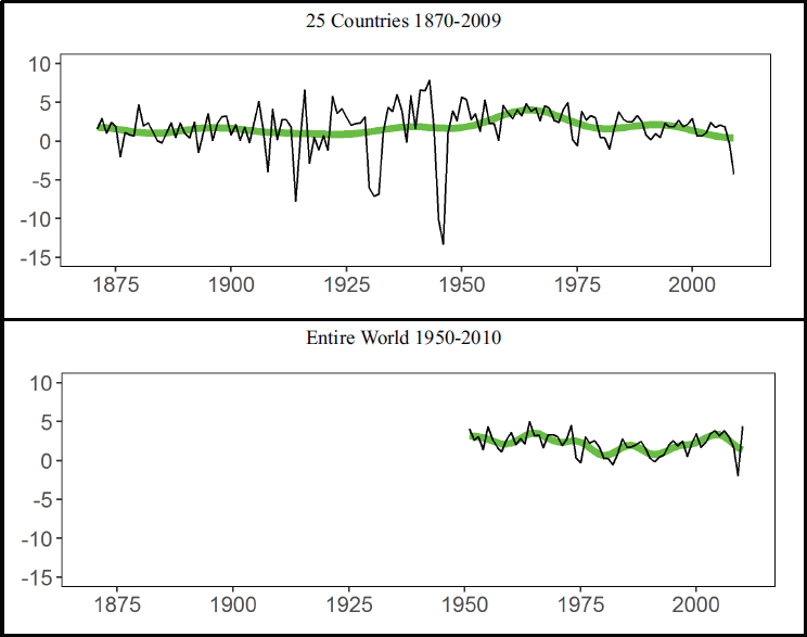
To apply the MW approach to the Maddison data, one must construct a univariate series for global growth rates. World GDP per capita is already aggregated and provided directly by the Maddison Project for 1950-2010. To construct the second series, the population tables provided by in the original Maddison data (through 2009) can be used to convert GDP per capita to GDP, which can be aggregated and then divided by the aggregate population of the 25 countries in this example. The growth rate is constructed by taking the first difference of the logs of aggregate GDP per capita. The resulting growth rates are shown in Table D-1 and in Figure D-1, which also displays the results of filtering out the short-run
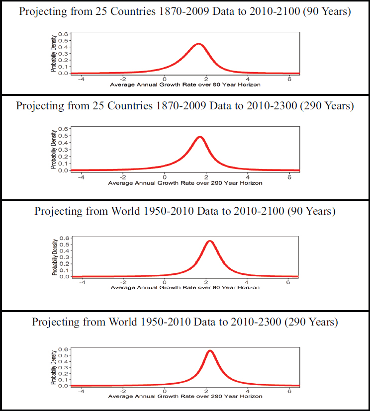
variation in the raw data. Figure D-1 also shows the long-run variation of the growth rates (i.e., with frequency less than qπ/T). The estimated predictive density is shown in Figure D-2. Summary statistics for this distribution are given in Table D-2.
TABLE D-1 Growth Rates of Aggregate GDP per Capita, in percent
| Year | 25 Countries 1870-2010 | Entire World 1950-2010 |
|---|---|---|
| 1871 | 1.58 | NA |
| 1872 | 2.93 | NA |
| 1873 | 1.04 | NA |
| 1874 | 2.40 | NA |
| 1875 | 1.94 | NA |
| 1876 | –2.04 | NA |
| 1877 | 1.10 | NA |
| 1878 | 0.80 | NA |
| 1879 | 0.64 | NA |
| 1880 | 4.66 | NA |
| 1881 | 1.98 | NA |
| 1882 | 2.34 | NA |
| 1883 | 1.27 | NA |
| 1884 | 0.11 | NA |
| 1885 | –0.24 | NA |
| 1886 | 1.04 | NA |
| 1887 | 2.34 | NA |
| 1888 | 0.50 | NA |
| 1889 | 2.36 | NA |
| 1890 | 0.97 | NA |
| 1891 | 0.42 | NA |
| 1892 | 2.48 | NA |
| 1893 | –1.48 | NA |
| 1894 | 1.09 | NA |
| 1895 | 3.55 | NA |
| 1896 | 0.06 | NA |
| 1897 | 2.31 | NA |
| 1898 | 3.13 | NA |
| 1899 | 3.23 | NA |
| 1900 | 0.80 | NA |
| 1901 | 2.15 | NA |
| 1902 | 0.07 | NA |
| 1903 | 1.81 | NA |
| 1904 | –0.20 | NA |
| 1905 | 2.50 | NA |
| 1906 | 5.13 | NA |
| 1907 | 1.45 | NA |
| 1908 | –3.95 | NA |
| 1909 | 4.13 | NA |
| 1910 | 0.20 | NA |
| 1911 | 2.77 | NA |
| 1912 | 2.72 | NA |
| Year | 25 Countries 1870-2010 | Entire World 1950-2010 |
|---|---|---|
| 1913 | 1.87 | NA |
| 1914 | –7.78 | NA |
| 1915 | 0.69 | NA |
| 1916 | 6.61 | NA |
| 1917 | –2.84 | NA |
| 1918 | 0.49 | NA |
| 1919 | –1.13 | NA |
| 1920 | 0.71 | NA |
| 1921 | –1.17 | NA |
| 1922 | 5.78 | NA |
| 1923 | 3.55 | NA |
| 1924 | 4.18 | NA |
| 1925 | 3.00 | NA |
| 1926 | 2.10 | NA |
| 1927 | 2.23 | NA |
| 1928 | 2.34 | NA |
| 1929 | 3.13 | NA |
| 1930 | –6.07 | NA |
| 1931 | –7.12 | NA |
| 1932 | –6.81 | NA |
| 1933 | 1.24 | NA |
| 1934 | 4.33 | NA |
| 1935 | 3.88 | NA |
| 1936 | 6.04 | NA |
| 1937 | 3.98 | NA |
| 1938 | –0.14 | NA |
| 1939 | 5.89 | NA |
| 1940 | 1.65 | NA |
| 1941 | 6.61 | NA |
| 1942 | 6.52 | NA |
| 1943 | 7.83 | NA |
| 1944 | 1.70 | NA |
| 1945 | –10.27 | NA |
| 1946 | –13.33 | NA |
| 1947 | 1.05 | NA |
| 1948 | 3.93 | NA |
| 1949 | 2.61 | NA |
| 1950 | 5.67 | NA |
| 1951 | 5.35 | 4.08 |
| 1952 | 2.72 | 2.65 |
| 1953 | 3.51 | 3.05 |
| 1954 | 1.27 | 1.42 |
| 1955 | 5.30 | 4.32 |
| 1956 | 2.26 | 2.70 |
| 1957 | 2.24 | 1.69 |
| 1958 | 0.10 | 1.12 |
| 1959 | 4.60 | 2.62 |
| 1960 | 3.70 | 3.65 |
| 1961 | 2.89 | 2.05 |
| 1962 | 4.09 | 2.84 |
| Year | 25 Countries 1870-2010 | Entire World 1950-2010 |
|---|---|---|
| 1963 | 3.22 | 2.14 |
| 1964 | 4.83 | 5.02 |
| 1965 | 3.88 | 3.16 |
| 1966 | 4.27 | 3.30 |
| 1967 | 2.63 | 1.65 |
| 1968 | 4.56 | 3.28 |
| 1969 | 4.23 | 3.35 |
| 1970 | 2.67 | 3.07 |
| 1971 | 2.43 | 1.91 |
| 1972 | 4.09 | 2.69 |
| 1973 | 4.97 | 4.52 |
| 1974 | 0.17 | 0.39 |
| 1975 | –0.59 | –0.26 |
| 1976 | 3.85 | 3.06 |
| 1977 | 2.70 | 2.24 |
| 1978 | 3.28 | 2.60 |
| 1979 | 2.95 | 1.74 |
| 1980 | 0.47 | 0.25 |
| 1981 | 0.44 | 0.26 |
| 1982 | –1.01 | –0.50 |
| 1983 | 1.52 | 0.86 |
| 1984 | 3.81 | 2.79 |
| 1985 | 2.79 | 1.70 |
| 1986 | 2.45 | 1.77 |
| 1987 | 2.52 | 2.04 |
| 1988 | 3.29 | 2.49 |
| 1989 | 2.52 | 1.51 |
| 1990 | 0.73 | 0.32 |
| 1991 | 0.22 | –0.16 |
| 1992 | 0.98 | 0.42 |
| 1993 | 0.49 | 0.74 |
| 1994 | 2.32 | 1.97 |
| 1995 | 1.84 | 2.58 |
| 1996 | 1.87 | 1.88 |
| 1997 | 2.70 | 2.51 |
| 1998 | 1.88 | 0.52 |
| 1999 | 2.27 | 2.30 |
| 2000 | 2.93 | 3.47 |
| 2001 | 0.62 | 1.70 |
| 2002 | 0.62 | 2.29 |
| 2003 | 1.09 | 3.47 |
| 2004 | 2.40 | 3.85 |
| 2005 | 1.78 | 3.18 |
| 2006 | 2.06 | 3.85 |
| 2007 | 1.87 | 3.08 |
| 2008 | –0.48 | 1.62 |
| 2009 | –4.31 | –1.96 |
| 2010 | NA | 4.39 |
NOTES: NA, not available. See text for explanation of the calculation.
NOTE: See text for discussion.
IMPLEMENTATION
The MATLAB code for implementing the MW approach is freely available from Mark Watson’s website.2 Only a subset of the code is required to generate the results presented below: lr_main_annual.m, figure_1_2.m, Sigma_Compute.m, den_invariate.m, psi_compute.m, t_mixture.m, and lr_pred_set.m. It is possible to replicate our estimates using the nine-step procedure detailed in the rest of this section.3
Step One
Alter the directory paths and file names in the code to point to the data.
__________________
2 See https://www.princeton.edu/~mwatson/wp.html [November 2016].
3 Note: these calculations were initially implemented in R but replicated in MATLAB using the MW files.
Step Two
Generate the q = 12 cosine transformations (the MW recommendation) and project the growth time series x of length T onto the space spanned by a constant (which picks up the unconditional mean of the series) and a set of q regressors that are cosine transformations of the data to isolate the low frequency variation in the data, denoted hereafter as the q × 1 vector X. Plot as depicted in Figure D-1 (above) (see the figure_1_2.m script).
Although a value of q = T would preserve all of the information in the original time series, MW recommend trimming it to q = 12. Truncating the set at q < T does involve some loss of information and thus some loss of econometric efficiency; a larger q would decrease the uncertainty in the predictions of growth rates. However, a larger q weakens the approximations utilized by this approach: the distribution of the transformed data would be further from the limiting normality and the shape of spectrum could exhibit greater deviations from the approximate shape near a frequency of 0 (the latter of which is not mitigated by a larger sample size T). According to the numerical calculations of MW, a value of q =12 tends to optimize the tradeoff between efficiency and robustness.
Step Three
Change the forecasting horizon(s) to the desired number of years (e.g., 90 = 2100-2010 or 290 = 2300-2010 in this application). Note that the available data for this example ends in 2009 or 2010, depending on the dataset, which is the year that the forecast begins.
Step Four
Specify the prior for the order of integration of the time series data generating process, denoted as d, on the near-0 spectrum by setting b = c = 0 in equation (20) of MW, which is the simpler prior that it discusses.
Step Five
Compute the q +1 dimensional covariance matrix Σ for each d (using the scripts Sigma_Compute.m and associated subroutines):
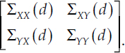
The particular value of d (along with q = 12 and the forecast horizon h/T) is a critical input into the computation of each Σ term, making each Σ term a complicated function of d as detailed in MW, Appendix A-4.
TABLE D-2 Summary Statistics of Uncertainty Distributions of Average Annual Growth Rates
| Horizon | 25 Countries 1870-2009 | World 1950-2010 | ||
|---|---|---|---|---|
| 2010-2100 (90 Years) | 2010-2300 (290 Years) | 2010-2100 (90 Years) | 2010-2300 (290 Years) | |
| Mean | 1.37 | 1.44 | 2.14 | 2.18 |
| Std. Deviation | 1.02 | 1.34 | 1.03 | 1.40 |
| 1st Percentile | –1.85 | –3.08 | –1.17 | –2.42 |
| 5th Percentile | –0.44 | –0.80 | 0.56 | 0.29 |
| 10th Percentile | 0.15 | 0.06 | 1.13 | 1.07 |
| 25th Percentile | 0.90 | 0.99 | 1.75 | 1.78 |
| 33rd Percentile | 1.13 | 1.23 | 1.91 | 1.95 |
| 50th Percentile | 1.49 | 1.58 | 2.18 | 2.20 |
| 66th Percentile | 1.78 | 1.85 | 2.42 | 2.45 |
| 75th Percentile | 1.96 | 2.04 | 2.60 | 2.64 |
| 90th Percentile | 2.42 | 2.63 | 3.13 | 3.31 |
| 95th Percentile | 2.78 | 3.20 | 3.59 | 3.99 |
| 99th Percentile | 3.71 | 4.89 | 4.95 | 6.26 |
The unobserved random variable YT is the average growth rate from time T + 1 to time T + h, relative to the observed average growth rate from t = 1 to T:
![]()
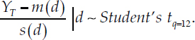
Conditional on d, the following statistic is distributed as a Student’s t with q = 12 degrees of freedom (see MW, equation (8)):
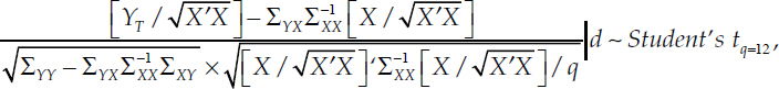
where the explicit dependence of each Σ term on d has been suppressed for the sake of notational brevity, mimicking MW. Note that ![]() is the mean predicted value of YT for each value of d, as implied by the symmetry of the Student’s t-distribution.
is the mean predicted value of YT for each value of d, as implied by the symmetry of the Student’s t-distribution.
Step Six
Compute the likelihood and posterior for d along a grid of n values, assuming a U[-0.4,1.0] prior following MW. One can then compute a predictive density for YT over a grid of values, averaging the conditional
density based on the above Student’s t using the posterior for d (see the lr_main_annual.m script).
Step Seven
Plot predictive distribution as Figure D-2 (see the figure_1_2.m script).
NOTE: See text for discussion.
Step Eight
Compute the summary statistics of the predictive distribution, shown in Table D-2, above. To further simplify notation, let m(d) and s(d) be such that:
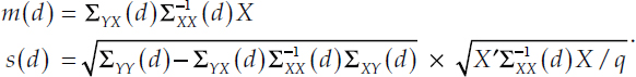
The mean growth rate can be computed by weighting the conditional means m(d) by the posterior for d, then adding to x1:T. To compute the percentiles, first substitute these variables into the above distributional result, making it clear that the distribution of YT given d can be written in terms of a Student’s t:
Note a ![]() has been cancelled in both the numerator and the denominator of the earlier expression. The unconditional cumulative distribution function of YT, that is, not conditional on d, is then given by the finite weighted sum of Student’s t-distributions:
has been cancelled in both the numerator and the denominator of the earlier expression. The unconditional cumulative distribution function of YT, that is, not conditional on d, is then given by the finite weighted sum of Student’s t-distributions:
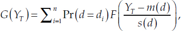
where F is the cumulative distribution function (CDF) of the Student’s t with q = 12 degrees of freedom.
The percentiles appearing in Table D-2 (above) of G(YT) can then be computed directly from the replication code associated with MW, using the t_mixture.m script. This script numerically inverts G(YT).
Step Nine
As discussed in Chapter 3, one could approximate the distribution of YT using three equally weighted values based on the tercile means. To compute the means of the terciles of average growth rate from time T + 1 to time T + h, shown in Table D-3, one would have to go beyond the MW analysis. Each tercile is defined as a range: from the 0th percentile (negative infinity) to the 33rd percentile is the lower tercile, from the 33rd percentile to 66th percentile is the middle tercile, and from the 66th percentile
TABLE D-3 Mean Growth Rate Conditional on Tercile of Uncertainty Distribution
| 25 Countries 1870-2009 | World 1950-2010 | |||
|---|---|---|---|---|
| Horizon | 2010-2100 (90 Years) | 2010-2300 (290 Years) | 2010-2100 (90 Years) | 2010-2300 (290 Years) |
| Bottom Tercile | 0.31 | 0.18 | 1.19 | 1.04 |
| Middle Tercile | 1.47 | 1.56 | 2.17 | 2.20 |
| Top Tercile | 2.33 | 2.57 | 3.07 | 3.31 |
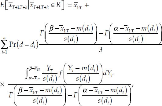
to the 100th percentile (positive infinity) is the top tercile. The expectation of the average growth rate from time T + 1 to T + h, conditional on the average growth rate falling in range R = (α, β), is
![]()
Substituting in the definition for the conditional expectation of YT:
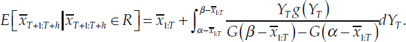
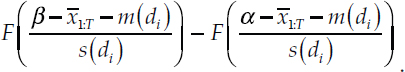
where g() is the pdf corresponding to G(). By virtue of α and β being the range of a tercile, the difference in the denominator will be equal to 1/3. Substituting in the full expression for the mixture of densities for g():

where f() is the probability density of a Student’s t with q =12 degrees of freedom.
Each term inside of the summation operator can then be scaled by the probability of being within the given tercile, conditional on d,
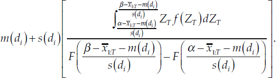
This is not necessarily 1/3: for some values of d, this will be more and for others, less. This allows us to include the corresponding reciprocal of this factor inside the integral:
where, again, F is the CDF for a Student’s t with q = 12 degrees of freedom. With a change of variables ZT = (YT – m)/s, the last term becomes:
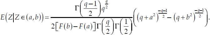
Notice that the bracketed term is just the expectation of a random variable ZT distributed as a standard Student’s t with q = 12 degrees of freedom, falling in the range
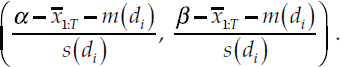
This term can be computed in closed form in terms of gamma functions and the CDF of the standard Student’s t-distribution with q = 12 degrees of freedom, which one can obtain from the work on truncated t-distributions by Kim (2008, p. 84):
REFERENCES
Kim, H.-J. (2008). Moments of truncated Student-t distribution. Journal of the Korean Statistical Society, 37, 81–87.
Mueller, U.K., and Watson, M.W. (2016). Measuring uncertainty about long-run predictions. Review of Economic Studies, 83(4), 1711-1740.
Summers, R., and Heston, A. (1984). Improved international comparisons of real product and its composition: 1950–1980. Review of Income and Wealth, 30(2), 207-219.


