
CHAPTER TWO
Setting the Stage
The current state of understanding on LCS dynamics is briefly summarized in this chapter through three sections describing the fundamental processes influencing the LCS, understanding the current state of observations and observational technology, and understanding the current level of predictive skill in terms of LC/LCE position, evolving structure, extent, and speed. The evolution of LCS research and associated fundamental theory is described in more depth in Appendixes A and B, respectively.
FUNDAMENTAL PROCESSES
The committee seeks to make recommendations to improve dynamic forecasts of the LCS (i.e., LC evolution and LCE formation, reattachment, separation, and propagation). To accomplish this, new observations—both sustained for regular, near-real-time assimilation by the forecast models, and short term for process studies that increase understanding of targeted processes—are key.
There have been many informative studies of individual processes in the Gulf, but few are of the LCS as a complete system or over a broad enough geographic area or study period that could be characterized as long term in nature. Long-term, comprehensive studies have been found to be among the most difficult to sustain, but once in place, they provide strong leverage for embedding additional short-term studies. For example, to date, satellite observations are the Gulf’s best long-term sources of oceanographic data, albeit for the surface only. Along-track altimeter data (SSH) are assimilated in near real time into models. Nevertheless, today, there is virtually no complementary near-real-time or long-term water column measurement set. This is critical in forecasting the LCS in that scientists do not fully understand the interaction between the boundaries (surface, inflow/outflow, and bathymetry) and the primary LC structure in the upper 1,000-meter range, or between the upper ocean (dominated by baroclinic processes) and the deeper ocean.
Within the LCS, when the LC is in its extended state (see Figure 2.1a), it will eventually spin off an anticyclonic eddy (see Figure 2.1b) that then propagates with significant current structure toward the west, after which the LC retreats (see Figure 2.1c). The interval at which an LCE separates varies considerably (about 0.5–19 months), but it
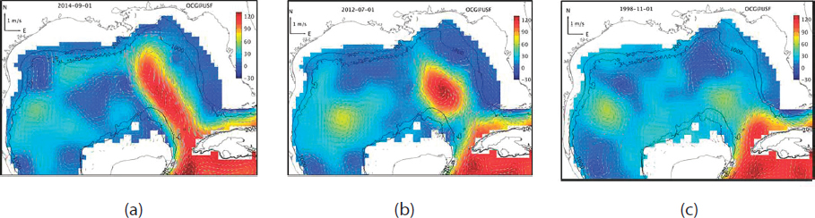
SOURCE: The figure is courtesy of Yonggang Liu and Robert Weisberg, College of Marine Science, University of South Florida. The observations derive from AVISO+ satellite sea level anomaly data produced by the Ssalto/Duacs with support from the CNES (Centre National d’Études Spatiales), and distributed by the CMEMS (Copernicus Marine Environment Monitoring Service), plus the mean dynamic topography MDT_CNES-CLS13. Further analyses include subtracting the domain average and estimating surface geostrophic currents from the sea level gradient similar to that in Liu, Y., R.H., Weisberg, S. Vignudelli, and G.T. Mitchum (2016), Patterns of the Loop Current system and regions of sea surface height variability in the eastern Gulf of Mexico revealed by the self-organizing maps, J. Geophys. Res. Oceans, 121, 2347–2366, http://dx.doi.org/10.1002/2015JC011493.
averages about every 8 to 9 months (Leben, 2005). There is some evidence of a higher probability of separation during the spring and fall (Hall and Leben, 2016), but there is notable variability in the timing of separations. In terms of mechanisms, Sturges et al. (2010) suggested that these separation events may be influenced by 20- to 30-day signals propagating upstream into the Gulf from the Carribbean Sea. This is based on observations of increased eastward transport through the Florida Straits, as well as increases in sea level on the offshore side of the LC flow in the weeks prior to a separation and builds on earlier work by Maul (1977). There is also evidence that cyclonic eddies along the LC front influence both LC extension and eddy separation (Gopalakrishnan et al., 2013; Schmitz, 2005; Walker et al., 2011). Bottom flows out of the Yucatan are also linked to eddy separation (Oey, 1996). Additionally, bottom topography is likely to have a role in LCS dynamics (e.g., Chérubin et al., 2005). Furthermore, the LCS sits in the Gulf, where atmospheric forcing may be important all of the time, not just during tropical cyclone passage (Judt et al., 2016). It would be useful to understand these processes and their influence on LCS behaviors at the air–sea interface.
General LCS discussions describe the LC forming as the Yucatan Current enters northward into the Gulf. In either its extended or retracted state, the LC exits by heading
east through the Florida Straits, where it feeds into the Gulf Stream. The relationships between inflow and outflow, and their impact on LC extension/retraction, are not fully understood, nor are counterflows and underflows in these areas, especially in the Yucatan Channel. These are important boundary conditions, and the linkages between their temporal variability and LCS state change are not fully understood or included in the physical expressions in the numerical models.
As the LCS evolves over time, there will be interactions with the unique bathymetry of the Gulf. The LC brushes by Mexico’s Campeche Bank as it enters the Gulf. As the LC extends north of 26°N, it encounters the deep Mississippi Fan, which shoals from 3,000 meters to 2,000 meters by 27°N and has an important influence on the LC interaction with deep eddies and topographic Rossby waves (TRWs). Once in the extended state, as the LC heads back south and then east toward the Florida Straits, it encounters the West Florida Shelf/Escarpment.
The direct impacts of shoaling depths on the LCS and the impacts of the deep mesoscale structures on the outer continental shelf are not well known. One interaction of the mesoscale circulation with bathymetry is the generation of TRWs. The generation processes are poorly understood, as are the consequences of the TRW energetics. The TRWs travel around the Gulf with the upslope bathymetry to their right, so their origin could be as far east as the southwest corner of the West Florida Shelf. Theories hypothesized over the years (Liu et al., 2016; Weisberg and Liu, 2017) postulate that there is an interaction between the LC’s position and bathymetry. One notion theorizes that the LC interacts substantively with a shallow area in the southwest West Florida Shelf, north of the Dry Tortugas, known as the “Pinch Point,” which can dampen or trigger an LCS extension and eddy formation (Liu et al., 2016; Weisberg and Liu, 2017). While there are gaps in understanding of both shelves that bind the LC, it is also important to know where the mesoscale eddies impact the oil exploration and production platforms in the western Gulf when the LC penetrates deep into the Gulf, or when the LCEs break off and propagate westward. Approximately 2 years of current data on Mexico’s Campeche Shelf are publicly available through BOEM’s 2009–2011 Loop Current Dynamics Experiment; the initial analysis on the variability of the LC along the Campeche Shelf break is described by Sheinbaum et al. (2016). In contrast with these other regions of topographic influence, there are/have been no similar moored time-series observations along the West Florida Shelf on which the LC regularly makes contact.
In summary, the fundamental physics questions to be answered with this campaign are specified in Box 2.1.
CURRENT STATE OF OBSERVATIONS AND OBSERVATIONAL TECHNOLOGY
LC observations have included a variety of methods (e.g., mechanical, thermal, chemical, acoustic, gravitational, electromagnetic, optical) and deployment strategies, including fixed structures (i.e., moorings, platforms, land-based installations) and moving platforms/instruments (i.e., ships, satellites, profilers, gliders, autonomous vehicles, mammals, drifters). The current status of surface and water column observational technologies considered for use in the Gulf are described here.
Surface Observations
Satellites
Satellites are required to provide broad spatial coverage of the sea surface for assimilation and adaptive sampling guidance. Altimeters provide along-track measurements of SSH. Imagers provide SST and ocean color.
Altimetric space-time coverage is dependent on the status of the international satellite altimeter constellation, including the number of satellites in orbit, and each individual satellite’s selected trade-off between cross-track spacing and repeat interval. Along-track altimeter data (SSH) is assimilated in near real time into models. Models then can assimilate deeper temperature/salinity (T/S) profiles that are synthetically constructed by considering SSH, SST, and deeper climatology. For example, the Navy Global Ocean Forecast System model uses the Modular Ocean Data Assimilation System (MODAS, an operational submodel that combines surface information with deep climatology) to synthetically extend the altimetric topography down into the water column. The Navy is currently testing an improvement to MODAS-created synthetic profiles, called ISOPs (Improved Synthetic Ocean Profiles). However, how an ISOP, once operational, can accept new near-real-time data from the upper 1,000 meters if it
becomes available is still unknown. Nevertheless, today, there is virtually no complementary near-real-time or long-term water column measurement set. In some models, along-track SSH data are first objectively mapped from multiple overpasses into mapped fields before assimilation.
A new National Aeronautics and Space Administration wide-swath altimeter, the Surface Water and Ocean Topography (SWOT) altimeter, has been proposed that will, when/if flown, provide a higher spatial resolution of the ocean surface topography than what was previously available. SWOT will provide high and unique resolution observations along its swaths (with an effective wavelength resolution of 15 kilometers as stated in the mission science requirement document), but will not be able to observe HF signals (for periods greater than 20 days). When combined with the array of traditional altimeters and subsurface measurements, a new capability in ocean forecasting will be available for assessment in data-rich areas.
Most radiometric imaging satellites provide multiple views of the Gulf for SST each day that the ocean surface is not obscured by clouds. The fast movement of cloud features in the atmosphere compared to ocean features has led to the development of image compositing techniques. Still, SST definition of the LC during the summer months is often difficult due to the intense solar heating of the surface. Tropical cyclones and storms can provide temporary views of the LC structure as the strong winds mix water across the relatively shallow thermocline on the outer edge of the LC, allowing the LC front to be defined until it is again masked by solar heating. Ocean color often helps discriminate between more productive coastal waters and less productive LC waters (again due to thermocline and hence nutricline depth), but the algorithms have more difficulty in humid regions like the Gulf, making the data most useful after the movement of frontal passages that move dry air over the Gulf.
Satellites for sustained wide-area observations combined with aircraft for enhanced event response are an effective combination for tracking LC position and surface current speeds, which has been demonstrated for decades in the Gulf.
HF Radar
HF radar has been used in the United States for the past 40 years to measure surface current speed and direction from a few kilometers up to 200 kilometers offshore. The HF radar network is organized as a quasi-national network within the National Oceanographic and Atmospheric Administration’s (NOAA’s) Integrated Ocean Observing System (IOOS) program, and is implemented regionally by nonprofit IOOS Regional Associations. There are nearly 180 HF radars registered in the national network, with
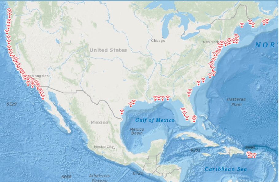
SOURCE: NOAA National Data Buoy Center. Courtesy of NOAA National Data Buoy Center.
about 150 of them reporting hourly data to the IOOS HF radar data assembly center (DAC). As shown in Figure 2.2, coverage is most concentrated on the U.S. West Coast and Mid-Atlantic. HF radar operations are principally supported in the NOAA IOOS budget. Initial procurement of HF radar sets and their installation has been enabled by a mix of federal and state funds. HF radar coverage in the Gulf of Mexico, however, lags behind the rest of the United States. Although Gulf HF radar coverage is sparse, its value was demonstrated in a small area: the shelf area of the northern Gulf generally south of Mississippi, Alabama, and the Florida Panhandle during the Deepwater Horizon oil spill (Harlan et al., 2010). The few existing Gulf HF radar installations are now located to continually observe the LC, its inflow/outflow, or LCEs.
Each HF radar site produces a map of what are known as the “radial” currents, which are the components of the surface current flowing toward or away from the radar. The radial current components from multiple adjacent radars are then combined to
produce a map of the “total” vector surface currents where overlapping coverage is available. Radial current data from individual HF radar sites are sent to the national HF radar DAC every hour, where the integration of the various data into total vectors takes place. The total vector fields are then made publicly available, although the radial data from individual radars are not.
Ocean modelers have demonstrated an ability to assimilate both total vector maps from a network and the radial component maps from individual radars. Assimilating the radial component maps has the advantage of expanding the area with surface current data beyond the regions of overlap. This will be especially important for HF radars placed on isolated offshore platforms or small islands where nearly 360-degree radial current coverage is possible, but overlap areas with adjacent HF radars are small or nonexistent. At present, however, the national HF radar DAC does not serve the radial data maps that go into the total vector maps. If the national HF radar DAC were to serve both radial and total vector current data, it would benefit HF radar assimilation nationwide. Until that time, the radial data from each new Gulf site (recommended in Chapter 3) can be set up to transmit directly to a dedicated data management location and to Gulf modelers for the greatest return on new HR radar investment.
Moored Buoys and Ocean Sensors on Fixed Platforms
Moored buoys are located in coastal and offshore waters, as shown in Figure 2.3a, and are used to measure air–sea interaction variables such as barometric pressure, wind speed and direction, air temperature, SST, wave energy spectra, and wave direction. These are principally meteorological buoys. Historic and near-real-time buoy data are available from the National Data Buoy Center (NDBC). Examination of the NDBC website shows several continually reporting NDBC-operated buoys and several buoys from other programs affiliated with IOOS and various universities. The NDBC website also depicts observational instruments mounted on fixed oil/gas field platforms (see Figure 2.3b). They can collect valuable air/sea surface data, but cannot be considered as continuous or regular reporting sites.
Ocean Surface Drifters
Surface drifters are backbone components of the industry-sponsored programs for LC monitoring and are also used for small-scale process studies. Early versions provided position and ocean temperatures through the Argo communication satellite network. Today, although drifters can be outfitted with a selection of near-sea surface oceano-
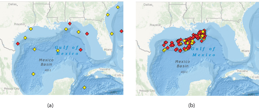
NOTE: The yellow diamonds indicate that data had been returned within the last 8 hours at the time the figure was created. Red diamonds indicate that no data had been returned within the last 8 hours at the time the figure was created.
SOURCE: NOAA NDBC.
graphic and atmospheric sensors, most operationally deployed drifters are inexpensive devices that communicate GPS positions to analysts on shore using the Globalstar and Iridium communication networks. The CARTHE Consortium (Schroeder et al., 2012) has demonstrated the efficacy of deploying large numbers of low-cost, biodegradable surface drifters for monitoring small-scale processes and oil slicks.
Large-scale drifting buoy deployment programs for monitoring surface currents in the Gulf of Mexico include those conducted by Horizon Marine, Inc. (HMI), a private-sector service provider to the oil and gas industry, and the CARTHE Consortium, a research organization funded by GoMRI for studying oil spill impacts on the Gulf’s ecosystems. HMI has deployed more than 4,300 Far Horizon Drifters in the Gulf and drogued at approximately 45 meters below the sea surface over the past 33 years as a part of their EddyWatch™ program for daily monitoring, analysis, and forecasting of ocean currents. The CARTHE Consortium was established in response to the 2010 Deepwater Horizon spill with the goal of guiding risk management and response efforts in the event of an oil spill. As part of the Grand LAgrangian Deployment (GLAD), the consortium has deployed more than 2,200 biodegradable surface drifters in the northern Gulf of Mexico
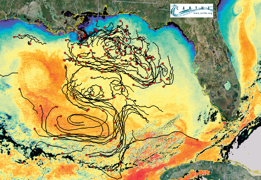
SOURCE: Tamay Özgökmen.
over the course of several expeditions, ranging from several weeks to months at a time (see Figure 2.4).
Water Column Observations
Acoustic Doppler Current Profiler (ADCP)
The ocean is relatively transparent to sound, and acoustic methods have been widely used to study Gulf currents. ADCPs, which measure the travel time of HF sound pulses, are often used, especially close to shore (e.g., Liu and Weisberg, 2005). They have a limited range (i.e., a few to hundreds of meters depending on frequency of operation)
and require “an adequate supply of suspended particles” to scatter the acoustic energy (Wunsch, 2015), but can be attached to moorings or fixed structures (looking either up or down) in a way that can capture a time series of partial or full water column current speed and direction measurements at predetermined depths of the instrument’s range. In accordance with regulatory requirements (U.S. Department of Interior [DOI] Bureau of Safety and Environmental Enforcement [BSEE] Notice to Lessees and Operators [NTL] No. 2005-G02 and subsequent renewals), currents within the upper 1,000 meters of water depth are required to be measured by ADCPs on operational Gulf of Mexico platforms; data are available through NOAA’s NDBC. ADCPs are a rather common feature on ship-based surveys, moorings, and buoys deployed by the scientific community in the Gulf, and the technology is moving forward rapidly to integrate ADCPs on autonomous platforms, such as surface vehicles and gliders.
Pressure-Recording Inverted Echo Sounders (PIES)
A sequence of BOEM (and its predecessor agency, the Minerals Management Service [MMS]) field studies from 2003 to 2011 used acoustic techniques to make observations using PIES. PIES instruments are deployed in a bottom-mounted array (typically tens of kilometers apart) together with near-bottom current meters to measure mesoscale features of the LCS (Cox et al., 2010; Donohue et al., 2006, 2008, 2016a,b; Hamilton et al., 2003, 2014). PIES instruments measure the round-trip travel times of regularly spaced acoustic pulses from the seafloor to the surface while simultaneously measuring pressure from a fixed platform on the seabed. The tidal signal is removed from the pressure, and the small residual pressure signal measures the variations due to deep eddies (Donohue et al., 2010). When data from an array of PIES are analyzed, they can determine temporal variability in the vertically integrated heat content (Talley et al., 2011). These data can be used to estimate thermocline depth and dynamic height. A PIES array can also determine geostrophic current changes and study the evolving eddy field (Talley et al., 2011).
PIES arrays, along with moored current meters, have been used in the Gulf (and in other field studies in other locations) and combined into a single instrument known as current PIES (CPIES). CPIES map the time-varying upper current and temperature structure to track TRWs and to study the dynamic coupling between the near-surface current structures and abyssal eddies (Donohue et al., 2010, 2016b). The deep currents were shown to be nearly depth independent (Hamilton, 2009).
An array that combined PIES instruments and current meter moorings was deployed in the central Gulf (Donohue et al., 2006; Hamilton et al., 2003), followed by small ar-
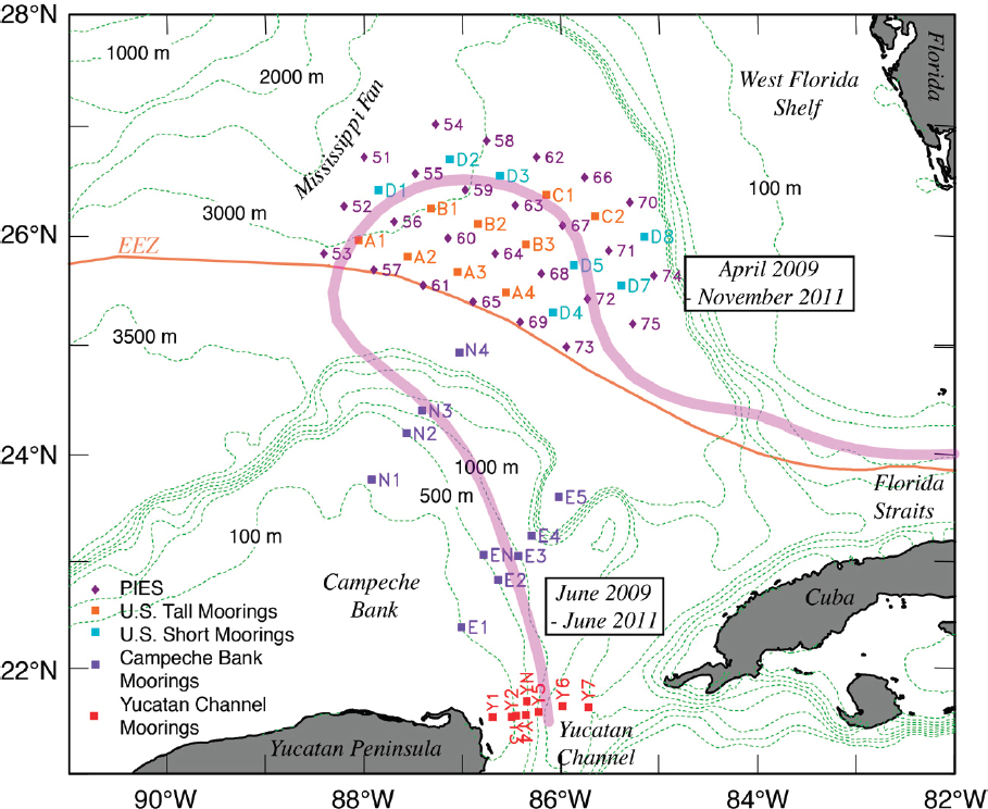
NOTE: The purple line shows the mean boundary (17-cm SSH contour) of the LC for the June 2009 to June 2011 interval.
SOURCE: Hamilton et al., 2014.
rays in the northwestern and northeastern Gulf (Cox et al., 2010; Donohue et al., 2008), leading to a field study of LC dynamics in 2009–2011 as shown in Figure 2.5 (Donohue et al., 2016a,b; Hamilton et al., 2014). The 2009–2011 array of PIES, plus separate current meters, was focused on the region where the LC was likely to form a narrow neck from which an LCE would likely separate. In all of these locations, the current records generated from the PIES data demonstrated excellent agreement of depths throughout the water column when compared with independent records on moorings (Donohue et al., 2016a).
Gliders
Underwater gliders profile vertically by changing buoyancy and traveling horizontally through the water on wings (Eriksen et al., 2001; Rudnick, 2016; Rudnick et al., 2004; Schofield et al., 2007; Sherman et al., 2001). Typically, underwater gliders may profile from the surface to 1,000 meters deep, completing a cycle from the surface to the given depth and back in 6 hours, while covering 6 kilometers horizontally. The resulting horizontal speed through water is therefore about 1 kilometers/h, or 0.25 meters/s. Mission durations of 3–6 months are common, producing several hundred profiles of the 1,000-meter depths over thousands of kilometers of track. Gliders come in several shapes and designs, but they are generally small (about 2 meters long) and light (about 50 kilograms), and may be easily deployed from vessels as small as an inflatable boat or as large as a global class research vessel. Much of the efficiency of gliders for sustained operations is realized through the use of small boats making repeated deployments and recoveries near the coast. Such sustained efforts have been going on for over a decade in a few locations in the Gulf.
Underwater gliders have carried a wide range of sensors; the main limitations are sensor power consumption and volume. As sensor power source volumes decrease and glider volumes increase, gliders will be able to carry more sensors, be more agile, and operate for longer durations.
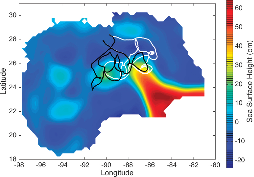
Figure 2.6 illustrates the path of two gliders that were deployed on December 9, 2011, and were recovered on April 19, 2012, to complete their 132-day missions (Rudnick et al., 2015). The glider tracks are shown superimposed on SSH (Leben et al., 2002), averaged over the first 90 days of 2012. One of the gliders (black line) was piloted to enter and exit the LC and an LCE. The other glider (white line) was piloted to find cyclonic eddies on the edges of the main currents. Two such cyclonic eddies were found, as seen by the spirals in the white track. These missions were part of a project that had gliders in the Gulf nearly continuously from 2010 through 2014. The two glider tracks shown in Figure 2.6 demonstrated a new level of skill and accuracy in glider operations, successfully navigating through the LC front and sucussfully measuring vertical structure within the LC itself.
Underwater gliders are a proven adaptive sampling platform for sustained collection of near-real-time subsurface profile data for the upper 1,000 meters in both deep water and coastal areas of the Gulf. Underwater glider capabilities are rapidly expanding, including operations in very shallow (10 meters or less), highly stratified coastal zones, and the extension in capabilities of deep gliders that are able to analyze full water column profiles in the Gulf. Hybrid gliders equipped with thrusters further expand the
operational envelope of these platforms. New sensors are constantly being integrated into glider platforms, including the Laser In Situ Scattering and Transmissometry sensor mandated to be deployed in response to the Deepwater Horizon oil spill. Likewise, dramatic increases in on-board energy may be available soon, in which case hybrid gliders could become much more useful in areas with high currents like the Gulf. These many options enable gliders to be customized for the most cost-effective use in the Gulf.
Profiling Floats
Profiling floats used in the Argo program deliver one conductivity-temperature-depth profile from the surface to 2,000 meters deep every 10 days. These floats are deployed globally for climate and general oceanographic data, with 3,800 floats operating at
this time. About 20 Argo floats are currently deployed in the Gulf of Mexico.1 There are other profiling float designs that are useful for specific scientific studies, such as biogeochemistry. For example, as with gliders, sensor capabilities that can be incorporated into profiling floats are expanding. Similar to gliders, profiling floats have demonstrated increased depth capabilities, all the way down to 6,000 meters. A profiler that uses acoustic methods for geolocation, used in a Gulf field study (Hamilton, 2009), is the RAFOS float. Rapid profiling capabilities also are being established by the U.S. hurricane forecasting community (Shay and Uhlhorn, 2008).
Surface Vessels
Surface vessels operated by a wide range of government, academic, industry, commercial and recreational fishing, diving, and private individuals are active in the Gulf. Some are dedicated to ocean exploration and observing; they can deploy and retrieve tethered or expendable instruments and autonomous vehicles. They are normally outfitted with hull-mounted and topside-installed sensors such as multibeam bathymetric sonar, ADCPs, SST sensors, and air temperature and pressure instruments. Nonscientific vessels can serve as “vessels of opportunity” to deploy instruments or autonomous vehicles. Dedicated oceanographic ships can be deployed to a specific area of interest and can either loiter in a spot or move to follow a feature. However, ships are expensive, costing tens to hundreds of thousands of dollars per day.
Airborne EXpendable BathyThermograph (AXBT)
Released by aircraft, these AXBTs measure temperature from the surface to approximately 350 meters below the surface. AXBTs are useful for determining the thermal structure in the upper ocean and for validation of modeling efforts. Like surface vessels, while they are agile, able to observe specifically designated areas, and report in real time, they also rely on aircraft. If the AXBT payload is large, they must rely on manned aircraft with high flight hour costs. The operational tempo for AXBT deployment must be characterized as episodic; it is useful when weather permits and can be additive in adaptive sampling schemes, but expense remains an issue.
___________________
1 See argo.ucsd.edu.
Autonomous Underwater Vehicles (AUVs)
AUVs have a wide range of scientific missions worldwide and rapidly expanding capabilities. Short-duration shipboard deployments (on the order of 24 hours) are most common, but recent missions up to 1 month in duration have been demonstrated. Improvements in on-board energy generation and storage are expanding the range and power and corresponding sensor capacity for AUVs. In the Gulf, AUVs are capable of sensing at all depths, and can be a useful augmentation to gliders and profilers.
Autonomous Surface Vehicles (ASVs)
ASVs provide an adaptive sampling surface platform for sustained data coverage across the air–sea interface or as a communication gateway between satellites and subsurface instrumentation. ASVs are available as a turnkey service from ASV companies or can be acquired and operated by a buyer/leasee. The ASV paradigm is evolving rapidly. Some ASVs resemble small conventional surface vessels (typically powered by diesel engines) but are controlled with on-board intelligence supplemented by remote human supervision. Such platforms have been used to gather data, and in a few cases, deploy (but not recover) gliders and floats. Other ASVs extract energy from the environment (waves, wind, and solar), and these are usually smaller platforms that are well suited to making observations over broad areas for extended periods of time. In addition to gathering data themselves, ASVs can act as mobile acoustic communication hubs that can interrogate certain specifically equipped water column and seafloor instruments and return those data immediately to shore via satellite.
Observational Moorings
Observational moorings can be instrumented in a variety of ways to measure oceanographic parameters through the full water column, and as they are fixed platforms, they offer a viable way to obtain long-term data, though this option is often cost-prohibitive. Moorings have been installed in the Gulf of Mexico to measure currents throughout the water column during targeted campaigns such as the 2009–2011 BOEM Loop Current Dynamics Experiment (see Figure 2.5), but very few moorings have been installed and maintained overall and even fewer have been operated for more than a few years. The exceptions are several arrays of moorings operated in Mexican and Cuban waters on the Bank of Campeche and across the Yucatan Channel and the Florida Straits (further explained in Chapter 3 and mapped in Figure 3.2).
Shell is leading the march toward new opportunities to use oil and gas infrastructure as platforms of opportunity to expand oceanographic measurements in deeper Gulf waters. Shell’s Stones mooring development, located about 3,000 meters deep and approximately 200 miles southwest of New Orleans, includes a standard oceanographic mooring, independent from the Turitella Floating Production Storage and Offloading facility. This mooring was deployed to measure currents in the upper 1,000-meter range in accordance with the BSEE NTL No. 2009-G02 for the lifetime of the Stones development (upward of 20 years). Shell has been building a public–private partnership with several universities, NOAA, and others to transform this existing structure into a deep-ocean observatory. The mooring line is serviced every 6 months, and data are made publicly available through NOAA’s NDBC and Gulf of Mexico Coastal Ocean Observing System. The idea of transforming regulatory moorings and potentially other oil and gas assets into scientific platforms could offer new opportunities to build observing capacity on the shelf and deep Gulf and obtain water column data (among other observations) that otherwise would be cost prohibitive and difficult to sustain over long periods of time.
CURRENT STATE OF MODELING AND PREDICTIVE CAPABILITY
Progress has been made since Hurlburt and Thompson’s (1980) pioneering work in modeling the LC and eddies in the Gulf of Mexico. Today, most models use finite-difference or finite-volume methods, but some models also use the finite-element method. They can be conveniently distinguished by their vertical grid system: layers (NLOM), z-level (MOM, MITgcm), terrain-following sigma-level (POM, ROMS, FVCOM), and hybrid (NCOM, HYCOM, MSEAS, SUNTAN). However, they also differ in detailed implementation of model physics, horizontal grids, differencing schemes, etc. Despite the model differences, similarities in their gross behaviors are found, mainly because they numerically approximate the same governing equations of motion. Features such as the LC eddy-shedding periods, eddy propagation, flow profiles in the Yucatan Channel, and production of deep cyclones under the LC are similar in the different models. However, there are several important details to be examined and contrasted. These include the simulations of TRWs, deep currents, inflow/outflow variability, LCS shelf–slope interaction, cyclonic eddies, and LC eddy-shedding dynamics. In recent years, several Gulf circulation modeling efforts have been funded by the GoMRI. Such efforts, however, mostly focus on the northern Gulf circulation, surface/subsurface transport processes, and shelf–estuarine interaction.
Progress has been made in predictive capability and data assimilation. So far, most modeling efforts to predict LC variation and its eddy shedding process apply primitive
equation numerical models. Some of these efforts have the capability of assimilating remote sensing observations and limited in situ observations. For example, Oey et al. (2005a) performed a study to predict the LC and its eddy frontal position. Yin and Oey (2007) applied the bred-ensemble forecast technique to estimate the locations and strengths of the LC and LC eddies from July to September 2005. Counillon and Bertino (2009) presented a small-ensemble forecast using the HYCOM to predict LC eddy shedding. Mooers et al. (2012) evaluated several different community ocean models’ performances at LC eddy shedding prediction using various prediction skill assessment methods in the report of the Gulf 3-D Operational Ocean Forecast System Pilot Prediction Project (GOMEX-PPP). The NCOM was also utilized for multiple applications in the Gulf of Mexico (e.g., Barron et al., 2006; Jacobs et al., 2014) and compared to other models within an ensemble forecasting framework (Wei et al., 2016). More recently, Xu et al. (2013) applied the local ensemble transform Kalman filter to the POM to estimate the states of the LC and LCE from April to July 2010. With the four-dimensional variation (4DVar) method, Gopalakrishnan et al. (2013) tested the prediction of the LCE shedding process using the MITgcm model. All of these studies are focusing on a single LCE or a small number of LCE shedding events. The lack of generality makes the assessment of these models’ predictability difficult (e.g., Mooers et al., 2012).
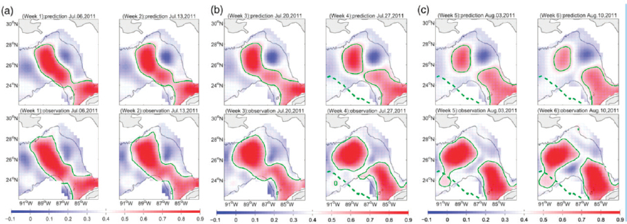
NOTE: Black lines are 1,000-meter isobaths. Red areas are the LC and LCEs. Green solid lines are 0.45-meter contours for observation, and 0.51-meter contours for prediction.
SOURCE: Reprinted from X. Zeng, Y. Li, and R. He. “Predictability of the Loop Current variation and eddy shedding 25 process in the Gulf of Mexico using an artificial neural network approach.” Journal of Atmospheric and Oceanic Technology. 2015. Vol. 32(5), pg. 1108.
The operational real-time global HYCOM and high-resolution Gulf of Mexico HYCOM models use the Navy Coupled Ocean Data Assimilation (NCODA) system (Cummings, 2005) to assimilate available satellite altimeter SSH and SST observations. These systems also assimilate vertical temperature and salinity profiles that are either measured in situ (when available) or synthetically constructed using climatological relationships between the SSH anomaly and a T/S profile, at depth, derived from the historical profile archives. The latter approach is known to misrepresent true subsurface density and energetic flow fields from time to time (Carnes et al., 1994; Cummings, 2005; Guinehut et al., 2004). Recent advancements in ocean variation and ensemble data assimilation methods, uncertainty prediction, and adaptive sampling with autonomous observation systems are expected to significantly improve model performance (see section on Data Assimilation and Numerical Modeling in Chapter 3) in forecasting LC events and dynamics.
In addition to primitive equation dynamic models, recent developments in statistical modeling based on long-term satellite observations are showing good potential in offering long-range LC forecasts (see Figure 2.7). Zeng et al. (2015a), for example, reported a novel method based on artificial neural network (ANN) and empirical orthogonal function (EOF) analyses to predict LC variation and its eddy shedding process. Validations against independent satellite observations indicate that the neural network-based model, in these trials, predicted LC variations and the associated eddy shedding process over a 4-week period. In some cases, a reliable forecast for 5 to 6 weeks may be possible. In the future, such statistical modeling and machine learning efforts can be merged with governing-equation-based ocean modeling (see Chapter 3). These are relatively new techniques that require more exploration and validation over longer periods of time.


