
6
Global Hydrological Cycles and Water Resources
INPUT SUMMARY
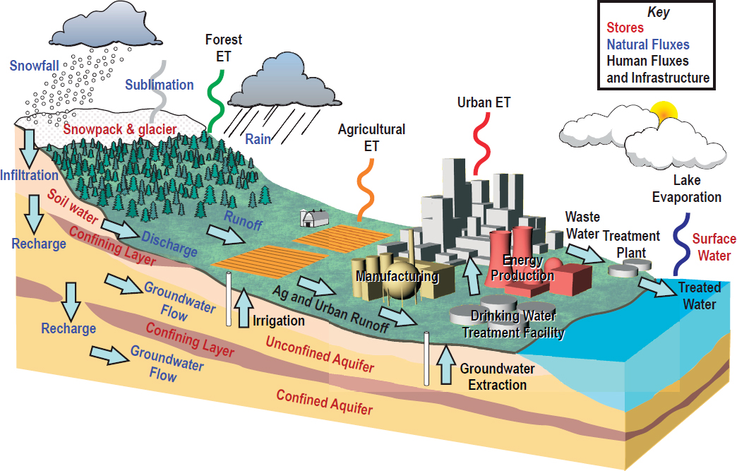
Water—the medium for life—shapes Earth’s surface and controls where and how we live. Chemical, biological, and physical processes alter and are altered by water and its constituents. Water is the most widely used resource on Earth, its mass nearly 300 times that of the atmosphere. On this foundation, humans add engineered and social systems to control, manage, use, and alter our water environment for a variety of uses and through a variety of organizational and individual decisions (Figure 6.1).
Therefore, understanding the hydrologic cycle and monitoring and predicting its vagaries are of critical importance to our societies. Remotely sensed data play a key role in advancing our insight about Earth’s water resources. Missions such as the Tropical Rainfall Measurement Mission (TRMM), Global Precipitation Measurement (GPM), Soil Moisture Active-Passive (SMAP), and the Gravity Recovery and Climate Experiment (GRACE)—along with sensors of the Earth Observing System (EOS)—including the Clouds and the Earth’s Radiant Energy System (CERES), the Moderate-Resolution Imaging Spectroradiometer (MODIS), the Advanced Spaceborne Thermal Emission and Reflection Radiometer (ASTER), the Atmospheric Infrared Sounder (AIRS), the Advanced Microwave Scanning Radiometers (AMSR-E and AMSR2), and lidar altimetry (Ice, Cloud, and Land Elevation Satellite, ICESat)—have provided important measurements of shortwave and longwave radiation, snow and glacier extent and change, soil moisture, atmospheric water vapor, clouds, precipitation, terrestrial vegetation and oceanic chlorophyll, and water storage in the subsurface, among many others. Visual, infrared, and lightning imagery from Geostationary Operational Environmental Satellites (GOES), especially GOES-16 and satellites in the GOES series through 2036, provide monitoring capabilities to improve nowcasting and warning for extreme storms and associated responses to hazards. Together, the Landsat 8 Operational Line Imager (OLI) and Thermal Infrared Sensor (TIRS), combined with the European Sentinel-2 satellites and the future launch of Landsat 9, will image Earth’s land area at 15-30 m spatial resolution every 3 days.
Future planned missions like Surface Water and Ocean Topography (SWOT) will measure surface water elevations in lakes, reservoirs, and large rivers, and NASA-ISRO Synthetic Aperture Radar (NISAR) will enable detection of surface disturbance by identifying subtle changes in surface elevation.
As a part of the Decadal Survey for Earth Science and Applications from Space, the Panel on Global Hydrological Cycles and Water Resources (Hydrology, or “H”) was tasked with identifying the high-level integrative questions in understanding the movement, distribution, and availability of water and how these are changing over time, and proposing the remote sensing measurements that will enhance and continue developments needed to address these questions and critical associated applications.
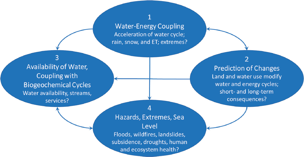
The chapter identifies four scientific and societal goals associated with the hydrologic cycle: (1) coupling the water and energy cycles; (2) prediction of changes; (3) availability of freshwater and coupling with biogeochemical cycles; (4) hazards, extremes, and sea-level rise. Scientific advances toward these four goals will support the development of societal mitigation for risks to the hydrologic cycle (e.g., contamination of drinking water supplies) or risks derived from the hydrologic cycle (e.g., floods and droughts).
Within each of the four scientific and societal goals, this chapter identifies key scientific quantifiable objectives that, when addressed, will advance our scientific understanding toward the scientific and societal goals. The quantifiable objectives serve as guideposts for identifying the scientific inquiries necessary
to achieve progress toward each of the four goals, and as such they provide the basis for the suggested enabling measurements. Just as phases of the hydrologic cycle are linked, the scientific and societal goals and quantifiable objectives are also linked. For example, simply quantifying the basic fluxes of the hydrologic cycle—precipitation, evaporation, streamflow, and groundwater flow—will enable progress on all four scientific and societal goals and many of the quantifiable objectives. The links between the quantifiable objectives are an important consideration for prioritizing the scientific and societal goals, the associated quantifiable objectives, and the resulting suggestions for enabling measurements.
The priorities of the panel are summarized in two tables. Table 6.1 lists the scientific and societal goals with the associated highest priority measurement objectives. The priorities listed in the following table are classified as Most Important (MI), Very Important (VI), and Important (I). The minimum ranking is Important owing to the criticality of water resources to water and food security, economic prosperity, and the health of the planet.
Methods for monitoring and modeling of the water cycle, and their application to societal goals, cover the wide range of needs for a comprehensive understanding of the hydrologic cycle as they relate to freshwater availability, water quality for human health and ecosystem services, and prediction of extremes and hazards. These extend from the accurate quantification of water and energy fluxes at the river basin scale, to accurate snow water equivalent (SWE) measurements for water supply forecasting, to improved drought monitoring, to flash flooding hazard prediction, to changes in land use and water quality in highly coupled human-natural systems. They also extend from recommendations to extend ongoing measurements, to new endeavors in detecting the phase (rain or snow) of precipitation, to measuring evapotranspiration, to new fields for application of remotely sensed data, such as water quality, groundwater recharge, effects of urbanization, water-modulated biogeochemical cycling, and prediction of hazard chains. Our science and applications have relied heavily on data availability since the beginnings of remote sensing. Improvements sought mainly relate to water and energy fluxes at Earth’s surface—evapotranspiration, snow and ice melt, rainfall, snowfall, and recharge and withdrawal of groundwater.
Table 6.2 presents the priority targeted observables for the science and societal targets/objectives the panel ranked as Most Important or Very Important.1 The information is taken from the subsection titled Enabling Measurements.
Implementing this program will enable the following scientific and applications advances:
- Improve monitoring of precipitation and evapotranspiration, with the goal to measure and model each so that the accuracy of the estimation of their difference is less than the rates of runoff or groundwater recharge:
- Especially for rates of precipitation of mixed water and ice, so as to estimate snowfall as well as rainfall; and
- In measurement and modeling of convective and orographic precipitation.
- Improve measurement and modeling of albedo of the components of Earth’s land surface—snow, ice, vegetation, and soil—to enable closing of the surface radiation balance to within 10 percent of the magnitude of the absorption:
- Necessary to model evapotranspiration, snowmelt, and retrospective reconstruction of the snow water equivalent.
- Understand how human modification of the land surface affects evapotranspiration, and the consequences for the hydrologic cycle.
- Understand how hazards in mountainous terrain and along coasts relate to weather extremes.
___________________
1 Not mapped here are cases where the targeted observables may provide a narrow or an indirect benefit to the objective, although such connections may be cited elsewhere in this report.
TABLE 6.1 Summary of Science and Applications Questions and Their Priorities
| Science and Applications Questions | Science and Applications Objectives (MI = Most Important, VI = Very Important, I = Important) | |
|---|---|---|
| H-1 | Coupling the Water and Energy Cycles. How is the water cycle changing? Are changes in evapotranspiration and precipitation accelerating, with greater rates of evapotranspiration and thereby precipitation, and how are these changes expressed in the space-time distribution of rainfall, snowfall, evapotranspiration, and the frequency and magnitude of extremes such as droughts and floods? |
(MI) H-1a. Develop and evaluate an integrated Earth system analysis with sufficient observational input to accurately quantify the components of the water and energy cycles and their interactions, and to close the water balance from headwater catchments to continental-scale river basins.
(MI) H-1b. Quantify precipitation rates and phase (rain and snow/ice) worldwide at convective and orographic scales suitable to capture flash floods as well as processes at longer and larger spatial scales. (MI) H-1c. Quantify rates of snow accumulation, snowmelt, ice melt, and sublimation from snow and ice worldwide at scales driven by topographic variability. |
| H-2 | Prediction of Changes. How do anthropogenic changes in climate, land use, water use, and water storage interact and modify the water and energy cycles locally, regionally, and globally, and what are the short- and long-term consequences? |
(VI) H-2a. Quantify how changes in land use, water use, and water storage affect evapotranspiration rates, and how these in turn affect local and regional precipitation systems, groundwater recharge, temperature extremes, and carbon cycling.
(I) H-2b. Quantify the magnitude of anthropogenic processes that cause changes in radiative forcing, temperature, snowmelt, and ice melt, as they alter downstream water quantity and quality. (MI) H-2c. Quantify how changes in land use, land cover, and water use related to agricultural activities, food production, and forest management affect water quality and especially groundwater recharge, threatening sustainability of future water supplies. |
| H-3 | Availability of Freshwater and Coupling with Biogeochemical Cycles. How do changes in the water cycle impact local and regional freshwater availability, alter the biotic life of streams, and affect ecosystems and the services these provide? |
(I) H-3a. Develop methods and systems for monitoring water quality for human health and ecosystem services.
(I) H-3b. Monitor and understand the coupled natural and anthropogenic processes that change water quality, fluxes, and storages, in and between all reservoirs, and the response to extreme events. (I) H-3c. Determine structure, productivity, and health of plants to constrain estimates of evapotranspiration. |
| H-4 | Hazards, Extremes, and Sea-level Rise. How does the water cycle interact with other Earth system processes to change the predictability and impacts of hazardous events and hazard chains (e.g., floods, wildfires, landslides, coastal loss, subsidence, droughts, human health, and ecosystem health), and how do we improve preparedness and mitigation of water-related extreme events? |
(VI) H-4a. Monitor and understand hazard response in rugged terrain and land margins to heavy rainfall, temperature and evaporation extremes, and strong winds at multiple temporal and spatial scales.
(I) H-4b. Quantify key meteorological, glaciological, and solid Earth dynamical and state variables and processes controlling flash floods and rapid hazard chains to improve detection, prediction, and preparedness. (I) H-4c. Improve drought monitoring to forecast short-term impacts more accurately and to assess potential mitigations. (I) H-4d. Understand linkages between anthropogenic modification of the land, including fire suppression, land use, and urbanization, on frequency of and response to hazards. |
TABLE 6.2 Priority Targeted Observables Mapped to the Science and Applications Objectives That Were Ranked as Most Important (MI) or Very Important (VI)
| Priority Targeted Observables | Science and Applications Objectives |
|---|---|
Surface Characteristics
|
H-1a and H-2a. Estimate rates of evapotranspiration and quantify how land use affects them. H-1c. Measure snowmelt, ice melt, and sublimation from snow and ice. |
| Snow Depth and Snow Water Equivalent (SWE) | H-1c. Quantify rates of snow accumulation, and track snowmelt. SWE = depth × density, but depth is the main contributor to spatial variability. |
Soil Moisture
|
H-1a and H-2a. Measure rates of evapotranspiration and quantify how land use affects them. |
| Precipitation and Clouds | H-1b. Improve identification of precipitation phase and rates of precipitation, especially when ice is present, and capture rainfall at orographic and convective scales. |
| Terrestrial Ecosystem Structure | H-2a. Improve the estimation of evapotranspiration. |
| Temperature, Water Vapor, Planetary Boundary Layer (PBL) Height | H-2a. Improve the estimation of evapotranspiration and sensible heat exchange. |
| Aquatic-Coastal Biogeochemistry | H-3a. Support emerging efforts to remotely sense water quality. |
| Surface Deformation and Change | H-4a. Monitor hazards and response in rugged terrain and land margins. H-1a and H-2. Monitor elastic and inelastic subsidence related to groundwater withdrawals. H-1c. Estimate snow density using interferometric Synthetic Aperture Radar (SAR) measurements. |
| Ice Elevation | H-1c. Help quantify rates of ice melt in basins where glaciers contribute significantly to runoff. |
NOTE: Summary text is included in the second column to illustrate the types of knowledge needed to achieve the objectives.
With growing populations, the demands on our water resources are increasing. The study of our hydrologic cycle, and how it changes over time, is critical to understanding and quantifying freshwater availability, water quality and ecosystem health, and anticipating and managing risks due to extremes. Remotely sensed data have permitted the scientific community to develop broad new understandings of the water cycle at scales from small basins to continents and the entire Earth, and to advance socially important applications. This chapter’s priorities will, if implemented, support and enhance the continuation of that work for the benefit of society and for a safe and prosperous future.
INTRODUCTION AND VISION
Motivation and Context
Water is the most widely used resource on Earth, and unlike other natural resources, water is a ubiquitous solvent and a medium for life itself. Fluxes of water connect the land to the atmosphere and the oceans. Water mediates Earth’s energy budget in the form of clouds, and it acts as a universal transport agent moving energy in the form of latent heat and all types of materials from sediments to bacteria across the planet (Evenson and Orndorff, 2013). The hydrologic cycle involves many processes (precipitation as rain or snow, evapotranspiration and evaporation, snowmelt, condensation, sublimation, surface runoff, infiltration, percolation, and groundwater flow) whereby water circulates between the atmosphere, land surface, and the oceans. To understand the physical structure, chemistry, biodiversity, and productivity
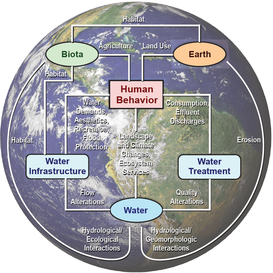
of the biosphere, it is important to know how water moves and how water is stored in the Earth system (NRC, 2012). Further, the movement of water influences Earth’s biogeochemical cycles and Earth’s climate (Vitousek et al., 1997). As Figure 6.2 shows, all components of the water cycle are linked at scales ranging from global to small basins, impacting and being impacted by human activities such as water withdrawals for agriculture and infrastructure development such as dams (Dalin et al., 2017).
The management of water resources is crucial for ensuring public health (Seid-Green, 2016) and securing the supply and allocation of water and food production to support human well-being, while sustaining healthy ecosystems. This is a major challenge for the 21st century (Poff et al., 2016). Opportunities exist, however, to integrate ecological health and human water needs in a comprehensive way (Gleick, 2000). In the Anthropocene, it is increasingly important to incorporate the human dimensions of freshwater use, to understand and predict aspects of freshwater resources (Konar et al., 2016).
Beginning with the launches of Sputnik in 1957 and Explorer 1 in 1958, remote sensing provided an opportunity to observe the Earth system, especially its water cycle, and its changes in space and time from a global perspective (Vince, 2011; Lettenmaier et al., 2015). Measurements from spaceborne and airborne platforms advance understanding of the hydrologic cycle and water resource assessment, which can improve society’s ability to manage water in our ever-changing world. To understand the dynamics of Earth’s terrestrial water cycle requires detailed in situ and remotely based measurements. Remote sensing has become a common tool in hydrology and water resources research, and because it enables a quantitative assessment of interconnections among multiple physical and biophysical and biogeochemical process across the world’s landscapes, it has enabled and catalyzed the advancement of Earth system science research and applications, and the fundamental role of the water cycle therein (McCabe et al., 2017).
The Earth observing systems that produce these sustained observations constitute vital national infrastructure, providing well-established, direct benefits to society and the economy, such as protecting life and property and securing food and water during disasters (Seid-Green, 2016). However, in spite of the importance of water to humanity, ecology, and environment, a comprehensive global hydrological observing system for monitoring the storage and movement of Earth’s water does not exist (Rodell et al., 2015).
The motivation for the Global Hydrological Cycles and Water Resources Panel’s work is to increase understanding of the hydrologic cycle from an integrated Earth system perspective. The intent is to provide a comprehensive perspective on the hydrologic cycle, including impacts and feedbacks at key coupled human-natural interfaces (water resources, agriculture, urbanization and infrastructure, natural resource use, and stewardship). The panel addresses its important task according to four distinct organizing themes that capture both scientific and societal imperatives: (1) coupling of water and energy processes between land and the lower troposphere; (2) prediction with a focus on variability, biogeochemical cycling, and extreme events; (3) water use and availability of quality water; and (4) hazards such as floods, droughts and related fires, landslides, and others that capture both scientific and societal imperatives.
This section, “Introduction and Vision,” provides the motivation and context for why the panel objectives are both scientifically compelling and societally important, and why now is a suitable time for investment into additional efforts to measure hydrologic parameters remotely using Earth observing satellites. The section then provides a review of the improvements in understanding, monitoring, and predicting hydrologic processes and resource assessment by Earth-orbiting satellites since the last decadal survey. The subsection “Challenges and Opportunities” identifies science and applications for which new or sustained measurements of hydrologic parameters are necessary to advance the hydrologic sciences and best serve society. The next section, “Prioritized Science Objectives and Enabling Measurements,” identifies and prioritizes 13 science and application objectives, which are categorized into broad societal questions based on coupled cycles, predicting change, water availability, and hazards. The subsection “Enabling Measurements” describes how these measurements can address the quantitative science objectives and questions. The section that follows, “Resulting Societal Benefit,” discusses priority measurements in the context of benefiting society, considering measurements that have broad application to water resource challenges such as availability of freshwater and hydrologic hazards.
Benefits of Prior Efforts
The previous decadal survey (NRC, 2007a), emphasized the need for high-quality global estimates of precipitation, soil moisture, and snow-water equivalent. In addition to these variables, the previous survey noted that measures of surface-water storage and transport would improve both modeling and an integrated understanding of the global water cycle. The four missions most relevant to the water cycle were:
- The already approved Global Precipitation Measurement (GPM) mission to provide estimates of precipitation;
- A soil moisture mission to address this crucial part of the land-surface water balance;
- A surface-water and ocean-topography mission to provide observations of water storage and associated variability; and
- A cold land processes mission to provide estimates of the water stored in snowpack.
Since that time, substantial progress has been made. Space-based observations of the hydrologic cycle and water resources have both improved scientific understanding and resulted in a variety of societal benefits. Some key achievements and transformational technologies include the following (Lettenmaier et al., 2015):
- The Global Precipitation Measurement (GPM) mission, which contributed to developing a capability to forecast floods and droughts and understand how precipitation patterns change through time across local to regional and global scales. GPM provides improved measurements to help improve weather and climate models (Skofronick-Jackson et al., 2016).
- The Gravity Recovery and Climate Experiment (GRACE), which contributed to the ability to measure the change in total water storage over large areas and information on global groundwater depletion (Alley and Konikow, 2015; Lakshmi, 2016; Famiglietti and Rodell, 2013; Richey et al., 2015).
- The Soil Moisture Active-Passive (SMAP) mission, which included improvements to water and climate forecasting, flood and drought monitoring, and predictions of agricultural productivity (Entekhabi et al., 2010). SMAP has been providing soil moisture observations that have been calibrated and validated at various locations (Chaney et al., 2016; Burgin et al., 2017; Colliander et al., 2017; Kim et al., 2017).
In addition to pertinent missions that have already launched, scheduled launches also represent substantial achievement to help understand the hydrologic cycle and provide societal benefits. The Surface Water and Ocean Topography (SWOT) mission, scheduled for launch in 2021, will provide both water surface elevations and extent and thereby information about surface-water storage and fluxes globally. The mission is expected to contribute to the understanding of individual lakes and reservoirs a few hundred meters in size and larger, and the information generated will aid the management of transboundary waters and ungauged basins (Biancamaria et al., 2016). The upcoming TROPICS mission—Time-Resolved Observations of Precipitation Structure and Storm Intensity with a Constellation of Smallsats (NASA EOS, 2017), to be launched in 2019—uses passive microwave spectrometry to provide for the first time high-revisit thermodynamic soundings and storm structure down to the boundary layer that can be integrated with high spatial resolution observations and rapid-refresh data assimilation systems to improve hydrological and hazard forecasts in remote regions generally and mid- and large-size ungauged basins (>300 km2).
Other recommended missions (NRC, 2007a) included the Snow and Cold Land Processes (SCLP) mission and the Hyperspectral Infrared Imager (HyspIRI) mission. SCLP’s objective is to measure the snow-water equivalent (SWE), snow depth, and snow wetness over land and ice sheets. As a third phase mission still in formulation, its status is conceptual, with newer approaches to measuring SWE addressed in this report. The HyspIRI mission was recommended as a second-phase mission for launch in the 2012 to 2016 period. Based on hyperspectral instruments designed to globally observe at high spatial and spectral resolution (Devred et al., 2013), such measurements provide an opportunity to assess ecosystem changes and functions, natural hazards such as volcanic eruptions and wildfires, and snow properties (Hook,
2014; Dozier et al., 2009). Since the last decadal survey, the mission concept has been refined to achieve needed measurements more economically, based partly on experience with hyperspectral observations of the lunar surface by the Moon Mineralogy Mapper (Green et al., 2011; Lee et al., 2015). Additionally, the ECOsystem Spaceborne Thermal Radiometer on Space Station (ECOSTRESS), with a planned launch of May 2018, provides NASA the opportunity to collect very high spatial (35 × 75 m) land-surface temperature (LST) at a 4-day temporal resolution. This measurement addresses the Objective H-1a measurement priority (“diurnal cycle of surface temperature [vegetation, soil, snow], at agricultural or topographic scales”) and can provide critical measurements that will help better design a spectrometry mission. To fully exploit the ECOSTRESS mission, its measurements plan needs to be expanded to cover all land areas rather than the current plan of selected regions and validation sites.
Challenges and Opportunities
Over the last 30 years, NASA’s Earth Observing System (EOS) transformed water cycle science and applications by providing—for the first time—frequent multiscale observations over large spatial domains across the planet. From the privileged vantage point of space orbits, coordinated missions such as the Afternoon Constellation (A-Train) and a developing suite of precipitation sensors rely on measurements from multiple satellites and collaborations with international partners, mainly space agencies and centers in Europe, Japan, and India to measure systematically key geophysical variables including shortwave radiation, atmospheric composition, clouds, precipitation, soil moisture, terrestrial vegetation and oceanic chlorophyll, water storage in the subsurface, and land subsidence, among many others, thus effectively establishing a de facto Earth Observing System. Such integrated observations show interrelatedness and feedbacks among seemingly removed processes and states, such as atmospheric composition and evapotranspiration, linking atmospheric pollution to clouds and surface temperature and water availability, and linking, in turn, public and environmental health to irrigation needs for food production and energy security.
NASA’s initiation of the EOS idea was foundational to the advent and growth of Earth system science and applications. Where lead time is paramount (e.g., seasonal climate for food production and water supply, 5-day weather forecasts for the construction industry, flashflood warnings for public safety, next-day snowfall for school closings), the integration of satellite-based observations and models through Data Assimilation Systems (DAS) significantly increased the predictability skill of existing forecast systems with implications for decision making under uncertainty across weather and water socioeconomic sectors (Magnusson and Källén, 2013; Bauer et al., 2015; Pagano et al., 2014; Bolten et al., 2010). An entirely new service industry developed over the last two decades to provide specialized value-added information products and client-based modeling and observing systems (Benson, 2012; Mandel and Noyes, 2012; NRC, 2003; Acclimatise, 2014).
In recent years, even as NASA’s original EOS missions surpassed expectations of longevity and utility, continuing to operate beyond their design life, the number of new satellite launches has declined and is split between improved continuation missions (e.g., GPM and GRACE-Follow On) and new missions (e.g., SWOT, NISAR). Benefiting from NASA’s early leadership in technological innovation, data access policy, and research and development, and more recently through international collaborations, the Program of Record (POR) of current and planned missions relies on mature (proven) technology to ensure essential data continuity. Yet, prompted by developments in sensor technology, high-performance computing, and scientific advances over the last decade, the current POR is inadequate for current and anticipated modeling capabilities, or to meet the data granularity and specific needs of data-driven decision making in the near future. This report proposes a measurement plan that addresses these needs.
PRIORITIZED SCIENCE OBJECTIVES AND ENABLING MEASUREMENTS
Science and Societal Goals, Questions, and Objectives
The linkages between the water cycle and freshwater availability, food and energy production, and environmental resilience highlighted in this decadal survey emerge from Grand Challenges of opportunity for a wide range of research programs (e.g., Trenberth and Asrar, 2014). Figure 6.3 and Table 6.1 summarize the goals, objectives, and assigned priorities from the details in this section. Quantifiable objectives and measurements (discussed in the next subsection) are intertwined, without a one-to-one mapping between them. Indeed, consistent with the ubiquitous role of the water fluxes connecting reservoirs and interfaces across the Earth system, many of objectives of lower priority would be achieved if specific higher priority objectives (Most Important or Very Important) are achieved.
H-1: Coupling the Water and Energy Cycles
Question H-1. How is the water cycle changing? Are changes in evapotranspiration and precipitation accelerating, with greater rates of evapotranspiration and thereby precipitation, and how are these changes expressed in the space-time distribution of rainfall, snowfall, evapotranspiration, and the frequency and magnitude of extremes such as droughts and floods?
Satellite-based observations available since 1979 have been used to generate multiple precipitation data sets (Ashouri et al., 2015; Xie et al., 2003; Adler et al., 2003; Xie and Arkin, 1997; Huffman et al., 1997; Xie et al., 2017) suitable for monitoring the water cycle at global scale. The frequency and space-
time patterns of rainfall, snowfall, snowmelt, soil moisture, and evapotranspiration control the water and energy cycles at basin, regional, and global scales. Changes in these patterns caused by climate change and human modification to the environment, coupled with increasing population and per-capita demand for water, pose significant challenges in the management of water-resources systems; threaten water, food, and energy security; challenge the health of ecosystems; and increase susceptibility to hazards and their socioeconomic consequences (e.g., Trenberth, 2011; Emori and Brown, 2005; Alexander et al., 2006; Min et al., 2011; Wentz et al., 2007). Changes in precipitation extremes, typically understood as the top 95th to 99.9th percentiles of daily accumulations, have been documented in many places (Alexander et al., 2006; Berg et al., 2013; Emori and Brown, 2005; Groisman et al., 2005; Kunkel et al., 2003), as well as in the duration of wet and dry spells (Zolina et al., 2013; Trepanier et al., 2015; Guilbert et al., 2015), and in the seasonality and phase (Barnett et al., 2005; Nayak et al., 2010). At the global scale there is large spatial variability with both negative and positive trends over large regions at multiple spatial scales (Ashouri et al., 2015; CHRS Rainsphere, 2017), with high uncertainty depending on the length of the available precipitation data records, both rain gauge observations and satellite products.
Accurately monitoring the timing, amount, phase (snowfall or rain), and vertical structure (hydrometeor composition) of precipitating systems globally and with sufficiently high spatial and temporal resolution to detect change and to quantify water availability at multiple scales from headwater catchments to continental river basins is an imperative challenge for the next decade. For basin-scale budget studies, estimating precipitation at spatiotemporal scales of 1 km and 1 hour are adequate, with temporal resolutions as fine as 5 minutes needed for urban flood warning and response (Berne et al., 2004; Emmanuel et al., 2012) and long-standing engineering design standards (Brown et al., 2009). Such observations will improve modeling of weather and climate, provide real-time warning for hazards such as floods and landslides, and increase the predictive understanding of teleconnections to attribute, anticipate, and manage environmental change.
Accurate estimation of precipitation amounts and detection of changes is challenging over land, especially over complex terrain (Barros, 2013). For example, High Mountain Asia (HMA) contains the largest deposit of ice and snow outside the polar regions; here, shrinking glaciers provide evidence of climate change in one of the world’s iconic regions, and the region plays a critical role in controlling the land-surface energy balance, and downstream irrigation and freshwater availability in several densely populated river basins (Kehrwald et al., 2008). In the past few decades a wide range of climatic changes, accelerated by economic developments and urbanization, has altered HMA’s radiation budget by increasing the temperature, depositing soot and dust in the snowpack that reduces its albedo, shifting the precipitation patterns, reducing snowfall, and amplifying the melting rate of glaciers and permafrost (Qui, 2008; Kaspari et al., 2014). HMA’s precipitation exhibits strong interannual variability (Barros et al., 2004; Lang and Barros, 2004; Barros and Lang, 2003), and its changes are still only poorly known because of the paucity of in situ observations and thereby the lack of validation of climate models. It is likely that future seasonal melting will shift the river peak flows toward the spring and decrease the water availability during the summer, posing risks to downstream water availability, impacting food and energy production and ecosystems (Immerzeel et al., 2010). This phenomenon and the lack of ground-based observations is not confined to HMA, but is evident in key mountain regions worldwide, leading to their designation as the Third Pole, which includes mountain ranges in North America, South America, and Europe (Stewart, 2009; Yao et al., 2012).
Whereas the linkages between climate variability and hydrological drought at interannual and decadal scales are well established (e.g., Barros et al., 2017), there is large uncertainty in assessing the sensitivity of drought frequency to observed changes in global temperatures (Sheffield et al., 2012; Dai, 2012; Trenberth et al., 2014). However, just as warmer temperatures increase the water holding capacity of the atmosphere, contributing to more extreme precipitation in some regions, higher temperatures—concurrent
with regionally lower humidity that leads to greater potential evapotranspiration—can result in increased drought severity due to persistent decreases in soil moisture, increased plant water stress, and degradation of plant productivity (Weiss et al., 2009; Easterling et al., 2000). Drought amplification by the interplay of concurrent and persistent high temperatures and low atmospheric moisture conditions is illustrated by Moran et al. (2014), who compared the Dust Bowl drought in the 1930s to the droughts in the 1950s and the early part of the 21st century in the western United States. They found that the 1950s drought was more severe than the 1930s and the early twenty-first-century droughts, even if the warm season temperature was only 0.68°C above the historic mean. Changes in post-drought ecosystem composition due to invasive species during recovery from recent “hot” droughts (Willis and Bhagwat, 2009) pose further challenges in managing the interplay between water, food, energy, and ecosystem services. Interestingly, drought “busting” events that replenish regional soil moisture and aquifers, including atmospheric rivers in the western United States (Dettinger, 2013) and land-falling hurricanes and tropical cyclones in the South and Southeast (Brun and Barros, 2014; Lowman and Barros, 2016), are also associated with major hazards and destructive damage in complex terrain and in urban areas because of heavy precipitation, extreme winds, flooding, and landslides (Guan et al., 2016; Waliser and Guan, 2017). The complex and nonlinear interconnections between water availability and water use, extreme events, and hazards encompass spatial scales ranging from 100 m to 1,000 km and temporal scales from minutes to years. They are iconic of the challenges presented to water cycle research, and a powerful motivation to monitor Earth at high spatial and temporal resolution, which can only be accomplished systematically from space.
Objective H-1a. Develop and evaluate an integrated Earth system analysis with sufficient observational input to accurately quantify the components of the water and energy cycles and their interactions, and to close the water balance from headwater catchments to continental-scale river basins.
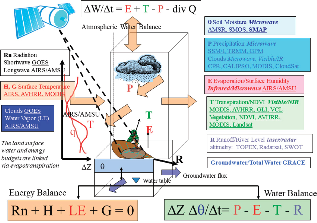
Figure 6.4 shows how the water and energy cycles are linked within the Earth climate system in many ways as well as how the various satellite missions have been used to observe these land and atmosphere variables. Objective H-1a underscores the need for a balanced research program combining observations and analysis systems. It also underscores the potential for scientific discovery that results from the integration of different observation types meeting requirements at distinct spatial and temporal resolution to probe interrelationships and feedbacks in the coupled Earth system.
For example, surface evapotranspiration (and its equivalent latent heat) are common fluxes to both water and energy cycles. However, point-scale evapotranspiration is directly measured by lysimeters, which mainly are installed in agricultural research settings, or estimated from measurements of sap flow in individual trees. It cannot be measured remotely. Instead, sensible and latent heat flux modeled from in situ measurements are the components of the surface available energy that are the primary drivers of the surface boundary layer that influences the coupling of the land with the atmosphere (Ek and Mahrt, 1994; Betts, 2004; Betts et al., 1996) and heats the surface air. Thus, the key to estimating evapotranspiration lies in measuring, or modeling, the variables and parameters that determine other terms of the energy balance equation—solar and longwave radiation, albedo, surface temperature, air temperature and atmospheric water vapor pressure in the boundary layer, and wind. Surface soil moisture influences the boundary layer cloud development through the latent heat flux associated with evapotranspiration, which in turn regulates surface temperature and thus the sensible heat flux and emitted longwave radiation, thereby affecting net surface radiation and available energy (Betts, 2004; Ek and Holtslag, 2004; Findell and Eltahir, 2003).
Quantifying the components of the water and energy cycles at Earth’s surface through observations and with sufficient accuracy to close water budgets over a wide range of river basin scales is a challenging problem that remains unresolved, but it is central to programs like the NASA Energy and Water System
(NEWS) and the World Climate Research Programme (WCRP) Global Energy and Water Exchanges (GEWEX) (Zhang et al., 2016; Rodell et al., 2015). With evidence of increasing climate variability and change (Barnett et al., 2005), and increased utilization of water resources (Oki and Kanae, 2006), understanding the controls on these components from an Earth system science perspective is imperative to assessing change, and to developing effective adaptation strategies.
These processes are explicitly included in climate models, where the surface water and energy cycles are closed (fluxes in balance) by mathematical design at model-resolved scales that are unfortunately much coarser than the governing process scales, which are therefore not appropriately represented (i.e., parameterized). Proper characterization of states and fluxes is complex and requires many parameters, including landscape and vegetation characteristics (e.g., topographic variability, soil properties, land use and land cover, vegetation biophysical parameters, water and land management, to name a few), most of which are poorly measured across the globe and whose effects are poorly understood. This results in high uncertainty and wide variability among predicted water and energy fluxes (Mueller et al., 2011; Rodell et al., 2015; Wild et al., 2015; Zhang et al., 2016) that limits our understanding to changes in water availability, the proper partitioning of evaporation and transpiration and storage, and the effect of the vertical distribution
of water vapor and cloud microphysics on precipitation among others that impact extremes like floods, droughts, and heat waves. For example, Chaney et al. (2016) used global FluxNet data to improve the process parameterization in the Noah land surface model. But of the ~650 sites in 30 regional networks covering 5 continents, only 253 eddy covariance stations with a total of 960 site-years of data at the needed 30-minute time resolution have been harmonized, standardized, and gap-filled (ORNL, 2007), with only 154 sites open to the community. Further evaluation and quality control of the data reduced the useable number to 85. Many regions (South America, Africa, Asia, and Australia) have fewer than 3 or 4 sites. The existing observational vacuum handicaps the science and can be addressed effectively only through remote sensing observations in the context of a broader integrated Earth system analysis.
What might comprise this context?
- Improved validation of remote sensing products through a significant increase in core sites (high-quality, multiple-variable measurements sites over ~10 × 10 km grids that can resolve subgrid flux heterogeneity at the 1 km scale or finer) and sparse validation sites measuring fewer locations or variables within a 10 × 10 km grid. This requires the coordination of space agencies and international bodies such as the World Meteorlogical Organization (WMO) and WCRP.
- Development of high-resolution Earth system models at spatial resolutions of 1 to 3 km, which can resolve watershed-scale water and energy states and fluxes with finer spatial heterogeneity and enable improved understanding and landscape management. Approaches could include elements such as the hyper-resolution land-surface modeling based on tiling of complex hydrologic response units, which offers one approach for continental modeling at 30 m (Chaney et al., 2016).
- Coordinated networks of in situ and remote sensing products that can improve the characterization of the land-surface energy fluxes, and resolve surface solar and longwave radiation balances within 10 Wm-2 accuracy at 1 km resolution globally, four times daily. Resolving the diurnal cycle is the desirable goal, but progress can be achieved through the integration of models and high-spatial resolution measurements at lower temporal resolution.
- The upcoming ECOSTRESS mission (launch 2018) on the Space Station can provide useful landscape-scale (~70 m spatial and 4-day temporal resolutions) top of the canopy temperatures. Likewise, ongoing efforts to produce 30 m multispectral harmonized surface reflectance products through the fusion of Landsat-8 (and Landsat-9 in 2020) and Sentinel-2a and -2b with high-revisit frequencies (~3-4 days at the Equator, and 1-2 days at midlatitudes) represent significant space-time resolution improvements over the highest resolution MODIS products currently available. Addition of a polar-orbiting imaging spectrometer to this constellation would enable spectroscopic interpretation and validation of the observations from multispectral sensors.
- Development of assimilation techniques and data analytics that can provide the desired integration and synthesis from merging in situ, remote sensing, and hyper-resolution models.
Given these advances, critical science and societal questions can be addressed, such as the following:
- What are the impacts of increased atmospheric CO2 and other greenhouse gases on the coupled water-energy-biogeochemical cycles, and do these modify water availability at basin to regional scales?
- To what extent have the water cycle components and their variability changed, and have these resulted in changes to extreme events (floods and droughts)?
- How will monitoring and modeling of water and energy balance variables at the basin and field scales lead to improved management practices and resiliency?
Objective H-1b. Quantify precipitation rates and phase (rain and snow/ice) worldwide at convective and orographic scales suitable to capture flash floods and beyond as well as processes at longer and larger spatial scales.
The Global Hydrological Cycles and Water Resources Panel assigned highest priorities to developing an Integrated Earth System analysis, which would integrate models and observations, and to measuring rainfall and snowfall and accumulated snow on the ground, which are key constraints and inputs into that analysis. Precipitation is the most important water flux in terrestrial hydrology, and thus precipitation measurements are key input variables in hydrologic and water resources models. Precipitation is equally important to a vast array of applications from agriculture, to ecosystem management, to climate monitoring and adaptation efforts, including risk-based engineering design of critical infrastructure from highways to water supply systems. For these reasons, precipitation has been at the forefront of NASA’s sustained mapping efforts at global scales along with NOAA ground-based radar networks for the continental United States.
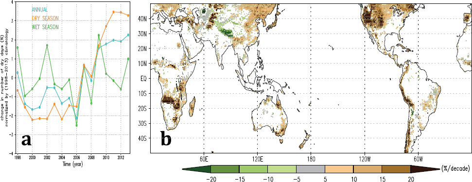
NASA, in collaboration with the Japanese Space Exploration Agency, JAXA, launched the Tropical Rainfall Measurement Mission (TRMM) in November of 1997 to quantify tropical rainfall and the associated latent heating structure. The mission success went beyond quantifying mean rainfall over the global tropical oceans, and it spurred the development of innovative algorithms that used the TRMM radars as a way to calibrate existing passive microwave radiometers and sounders as well as infrared observations to increase the spatial and temporal resolution of precipitation (Kummerow et al., 2015; Huffman et al., 2007). Figure 6.5 shows how TRMM detected significant drying trends from 1998 to 2013, especially in the western and central United States, Southern Africa, northeastern Asia, and southern Europe and the Mediterranean. These decreases are concurrent with positive trends elsewhere, resulting in spatial variability at the global scale and large regions of statistically significant negative trends along the midlatitude storm track in the northern Atlantic and positive trends in the maritime subcontinent (Nguyen et al., 2017).
The integration between a radar and sensors that provide wider spatial and temporal coverage was more fully developed in the second collaboration between NASA and JAXA precipitation efforts resulting
in the Global Precipitation Measurement (GPM) mission launched in February of 2014 (Hou et al., 2014). GPM not only extends the time series of climate-quality precipitation radar observations from TRMM, but it also extends the core satellite observational domain to high latitudes, and it formalizes the calibration concept developed during TRMM to make a consistent precipitation product from a global constellation of passive microwave and infrared sensors that can include models and both research and operational satellites to produce 5 km, 30-minute precipitation estimates globally. One key improvement in GPM over TRMM is the ability to predict global extreme precipitation. Whereas there is a 50 percent match between TRMM Level 3 precipitation and ground-based rain gauges for determining the extreme precipitation, this number rises to 60 percent for GPM (Huffman et al., 2017), demonstrating increased spatial (0.1 degrees versus 0.25 degrees) and temporal repeat (3 hours versus half hour) monitoring capability. This improvement in estimating extreme rainfall in ungauged regions of the world has important implications for engineering (Libertino et al., 2016; Olsen, 2015). The Integrated Multi-Satellite Retrievals for GPM (IMERG) combines precipitation estimates from all available passive microwave observations, with gaps filled using geosynchronous infrared precipitation estimates (Hong et al., 2004; Joyce et al., 2004; Hsu et al., 1997; Kummerow et al., 2015). These products are being produced today and are expected to continue improving as the community learns to more fully exploit the dual-frequency precipitation radars on GPM, as well as intercalibration procedures to the diverse instruments in the constellation (Berg et al., 2016). Further, by leveraging dual-frequency, dual-polarization radar measurements, improvements are expected in the detection and quantification of light and moderate rainfall that represent a significant fraction of the total precipitation, and in orbital mapping of three-dimensional (3D) storm structures at the mesoscale.
Precipitation is a multiscale process spanning a wide range of scales from the raindrop and raindrop cluster scales (µm to m) to the scale of storm cells (100 m to 10 km) to the scale of organized systems (~100 km; e.g., tropical cyclones, fronts). Continuity of passive microwave instruments, which currently provide the longest records of any geophysical variables derived from space observations, is essential to monitor the variability of global precipitation from decadal to interannual to daily time scales, especially over the world’s oceans, and to provide the large-scale context (regional to continental scale) to ongoing measurements of precipitation, soil moisture, sea ice, and other variables sensitive to water fluxes at the land- and ocean-atmosphere interfaces, including at short time scales, as high- revisit passive microwave spectrometry from space becomes available (e.g., TROPICS mission).
Numerous discussions within the precipitation community, reflected in multiple white paper submissions to this decadal survey, indicate the need and desire to continue to advance the quality of spaceborne instantaneous precipitation measurements not adequately covered by GPM, and to refine the spatial and temporal resolutions of precipitation estimates. For the latter, in particular, there is growing consensus that the key to success in this area is better process understanding coupled with assimilation into convection-resolving models that can provide continuous analyses and forecasts of precipitation at 1 km and 5 minutes to 1 hour scales, thus approaching the capabilities of ground-based radars over developed regions of the world today.
Advancing process understanding to properly model precipitation, particularly ice microphysics that can be gleaned from combined Doppler radar and radiometer information (Bryan and Morrison, 2012; Varble et al., 2014), or assimilate precipitation and its latent heating in convection-resolving models to forecast small-scale intense precipitation could possibly revolutionize how we view Earth observing satellites from standalone measurement platforms to integral components of coupled observing and modeling systems (Stephens and Kummerow, 2007). In the case of models with parsimonious microphysics, a strong case can be made that observing hydrometeor vertical velocities within the context of large scale environmental conditions, as established from reanalyses such as Modern-Era Retrospective Analysis for Research and Applications (MERRA; Rienecker et al., 2011), will provide useful constraints on microphysical parameterizations to
capture the vertical structure of precipitation in models that currently is lacking (Wilson and Barros, 2014, 2017), and thus to make high-quality, high-resolution, model-based analyses and forecasts of precipitation a reality. Advancing the quality of spaceborne instantaneous precipitation measurements does not require large leaps in technology, but rather innovation with regard to the development of multifrequency instruments and measurement strategies to significantly refine their horizontal and vertical resolutions. This will address continuing issues with orographic precipitation as well as improve the detection and quantification of shallow precipitation in complex terrain, snowfall, and light drizzle (Duan et al., 2015). A swath of 100 km is then needed for the calibration reference to operational microwave imagers, as well as operational sounders and visible and infrared imagers used in geostationary satellites.
Albeit complementary, snowfall (precipitation rate) and snow accumulation (precipitation amount) pose distinct measurement challenges. Snowfall accuracy at short time scales (minutes to hours) is critical for winter weather forecasting, with major implications for transportation and energy security applications, even leading to a snow impact scale for Northeast storms (Kocin and Uccellini, 2004). Currently, quantitative remote sensing of snowfall from satellites is largely limited to X- or W-band radar (Heymsfield et al., 2016; Kulie and Bennartz, 2009) for dry snow. Snow accumulation evolves from pulse contributions from a small number of individual storms with large interannual variability (Lang and Barros, 2004; Lundquist et al., 2013) to form snowpacks that grow in depth and spatial extent through the winter depending on environmental conditions and snowfall history. In the transition from the cold to the warm season, seasonal snow melts over a short period, weeks to several months, to produce runoff that is an essential source of freshwater resources in the foothills of high mountain regions and their adjacent plains such as the western United States (Bales et al., 2006). Not surprisingly, numerous reservoirs have been built to capture snowmelt runoff to further extend water availability.
The global volume of glaciers outside the polar ice sheets is also not accurately known owing to their uncertain thicknesses, but this number does not change as rapidly as SWE. Worldwide, snowmelt and glaciers support about two billion people (Mankin et al., 2015); mountain snowmelt and glaciers support over a billion (Barnett et al., 2005). In the mountains themselves, snowmelt provides essential soil moisture late into the melt season (Harpold and Molotch, 2015), and melting glaciers supply water throughout the melt season, which in some regions is otherwise a dry season. The global inventory of glaciers outside the polar ice sheets comprises 0.35-0.41 m sea-level rise equivalent (Radić and Hock, 2010; Grinsted, 2013), or 1.3-1.5 × 10¹⁷ kg. Compared to the global annual river runoff to the seas of ~4.4 × 10¹⁶ kg (Clark et al., 2015), the nonpolar glacier mass is equivalent to 3-4 years of global river runoff. Regionally and locally, annual glacier melt throughput, and the smaller magnitude net annual mass balance of glaciers, is extremely important for water resources and economies, especially for some arid and semiarid countries.
Albedo, areal extent (snow-covered area, SCA), and snow water equivalent (SWE) are important metrics of seasonal snow accumulation. The extent and albedo of seasonal snow govern the surface energy budget of large regions of the world at high latitudes and at high elevations, and therefore play a critical role in the water cycle of large regions of the world, with implications for the interannual variability of climate at global scales (Fletcher et al., 2009). Passive microwave estimates of SWE can succeed when radiative transfer models are coupled with snow hydrology models via data assimilation, but uncertainty and retrieval error increase significantly in complex terrain, when snow is wet, generally when SWE exceeds ~200 mm (deep snowpacks), and when tree canopy cover exceeds ~20 percent (Lettenmaier et al., 2015; Dozier et al., 2016). Measurements of snowfall, or of accumulated snow on the ground, constitute an important unsolved problem in the hydrology and water resources in most of the world. The next section addresses some approaches to this issue.
Objective H-1c. Quantify rates of snow accumulation, snowmelt, ice melt, and sublimation from snow and ice worldwide at scales driven by topographic variability.
As noted in the discussion of Objective H-1b, remote sensing of snowfall rate is difficult because of the huge difference in the dielectric properties between water and ice in the microwave spectrum. Even measuring snowfall at a meteorological station is difficult, because catching falling snow in windy conditions generally misses much of it (Yang et al., 2005). Instead, our historical knowledge of the distribution of snow accumulation comes from measurements of the snow on the ground, either by manual surveys (Armstrong, 2014; Church, 1933) or by snow pillows that sense the weight of the overlying snowpack (Cox et al., 1978). In mountain regions, where much of the snowpack in the middle and lower latitudes lies, topographic heterogeneity along with deep snow causes substantial uncertainty in our assessment of a major component of the hydrologic cycle. Even in regions like the western United States with an extensive snow pillow network, the pillows are on nearly flat terrain and in most basins do not cover the highest elevations, so in some years they poorly represent the spatial distribution of the snow and the total volume of water stored in the basin’s snowpack (Bales et al., 2006). In the river basins of California’s Sierra Nevada, for example, the interquartile error in the forecast of the April-July runoff is 213 percent to 135 percent, but the error distribution has long tails, both positive and negative (Lettenmaier et al., 2015). In the world’s great mountain ranges, where surface data are sparse, precipitation estimates from lowland measurements, numerical weather models, or changes in sizes of glaciers span a large range of uncertainty (Kääb et al., 2012; Kapnick et al., 2014). This is further complicated by the fact that at high elevations, snowfall input is highly intermittent and typically associated with specific types of storms and regional conditions (Lang and Barros, 2004). Therefore, seasonal snow accumulation and snowpack conditions strongly depend on local interstorm hydrometeorology and occasional rain-on-snow events (GuanWaliser et al., 2016), which control snowpack evolution between snowstorms.
At mid- and high latitudes, including the Arctic and sub-Arctic regions, complex topography (and landform) also plays a critical role in the spatial organization of snow accumulation as well as snowmelt dynamics at the transition between the cold and warm seasons, impacting snow cover extent and duration, snow water equivalent, and albedo, which feed back into regional and global climate (Derksen et al., 2012). Although significant progress has been achieved to estimate snow water equivalent from passive microwave observations (Kelly and Chang, 2003; Li et al., 2015; Shi et al., 2016) and also using coupled physical and passive microwave models (Kang and Barros, 2012; Langlois et al., 2012), the spatial resolution generally is too coarse for hydrological and eco-hydrological research and applications. A promising new development addresses the resolution limitation by taking advantage of overlapping footprints, to bring spatial resolution at 36 GHz down to ~3 km at the expense of some reduction in signal-to-noise performance (Long and Brodzik, 2016). Other shortcomings of passive microwave retrievals of snow water equivalent remain, particularly its low saturation threshold of about 200 mm SWE (Dozier et al., 2016; Lettenmaier et al., 2015).
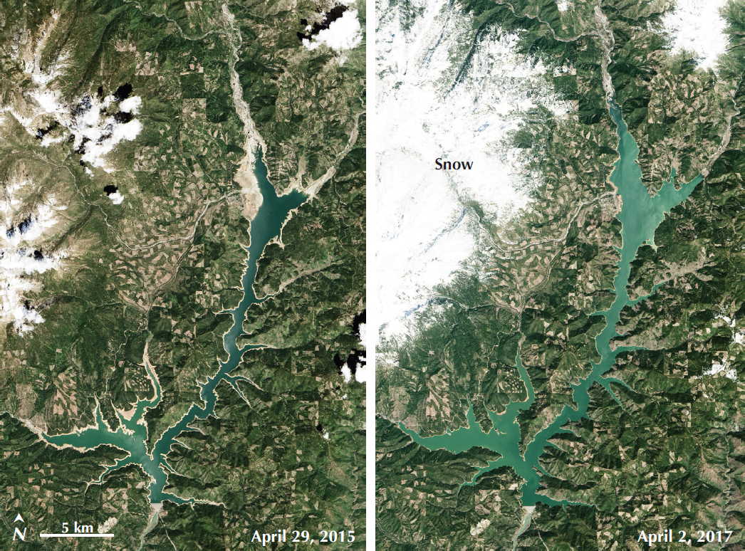
In regions like High Mountain Asia, the sparse measurement network supports neither seasonal runoff forecasts nor validation of precipitation models. In regions like the western United States, where in situ measurements and snow-depth measurements from airborne lidar are available, validation of snowpack resources computed with numerical weather models, such as the Snow Data Assimilation System (SNODAS; NSIDC, 2016), show discouraging results with significant under- and overestimates (Clow et al., 2012; Hedrick et al., 2015; Bair et al., 2016). Figure 6.6 shows the importance of snowmelt in the water supply of the western United States. Three years of drought from 2013 through 2015 brought California’s reservoirs and groundwater to historically low levels. The storms in the winter of 2017 replenished the reservoirs, but the groundwater remained depleted because of the extensive pumping during the drought (Margulis et al., 2016). Forecasts of the snowmelt runoff are based on a network of surface measurements, but because the sites seldom cover the highest elevations, as pointed out earlier, considerable snow amounts remain on the ground even after point-scale sensors indicate snow-free conditions (Rittger et al., 2016). The sta-
tistically based forecasts on average perform acceptably well, but occasionally generate errors of nearly a factor of two (Dozier, 2011). Therefore, estimating the spatial distribution of SWE in mountainous terrain, characterized by high elevation, steep slopes, and spatially varying topography, is an important unsolved problem in mountain hydrology.
Coupled with the problem of knowing the total quantity and spatial distribution of the snow accumulation are measuring and predicting its rate of melt, relating the rate of melt to environmental drivers, and the consequences of the rate and distribution of melt for water resources, glaciers, and ecosystems. The main drivers, absorption of solar and longwave radiation, vary with the solar geometry, atmospheric scattering and absorption, and illumination variability caused by topography (Marks et al., 1992; Marks and Dozier, 1992). Estimating these surface fluxes is also crucial to Objective H-1a, which requires addressing the
components of the surface energy balance. As with any process driven partly by absorbed solar radiation, variability in snow albedo causes variability in the rate of melt.
For surfaces with high albedo (a), an error in the measurement of albedo leads to a greater proportional error in absorption of the solar radiation (absorption = 1 – a, so for greater values of a closer to 1.0, a small error in a causes a greater proportional error in 1 – a). Changes in snow albedo are tied to changes in snow microstructure, specifically grain growth that reduces snow albedo at wavelengths beyond about 1 µm, and contamination by absorbing aerosols like dust and soot (Warren, 1982). These issues are included in the discussion of Objective H-2b.
H-2: Prediction of Changes
Question H-2. How do anthropogenic changes in climate, land use, water use, and water storage interact and modify the water and energy cycles locally, regionally, and globally, and what are the short- and long-term consequences?
Objective H-2a. Quantify how changes in land use, water use, and water storage affect evapotranspiration rates, and how these in turn affect local and regional precipitation systems, groundwater recharge, temperature extremes, and carbon cycling.
Humans have altered the landscape by changing the vegetation cover over centuries, but with increasing intensity over the latest decades. As a result fluxes in the water cycle have already changed. Specifically, the evapotranspiration flux and the terrestrial surface water budget have changed dramatically over the historical record as a result of human alteration of the landscape. Because sensible and latent heat fluxes are fundamentally coupled by thermodynamics, these changes have already had significant impact on the terrestrial surface energy budget, including surface temperature and outgoing longwave radiation.
The large enthalpy of vaporization (2.5 × 10⁶ J/kg) makes the latent heat flux due to evaporation a major term in the surface energy balance. Only one-fifth of the solar energy available to the Earth system is directly absorbed in the atmosphere. Half of the solar energy is first absorbed by the surface, and then latent heat flux and longwave radiation transfer it to the atmosphere. The latent heat flux is the most efficient dissipation mechanism available to return the surface to thermodynamic equilibrium upon solar forcing, and a major mechanism in zonally redistributing energy from the tropics, including the tropical oceans, to the higher latitudes. Latent heat flux and variations in it due to limiting factors over land such as availability of soil moisture are thus a major factor in the thermal forcing of the atmosphere at its base. It is also a source of moisture for the atmosphere that plays an important role in the formation of clouds, development of convection, and ultimately precipitation from local to regional scales (Aragão, 2012; Sun and Barros, 2014). By its control over buoyancy generation and moisture supply at the base of the atmosphere, evapotranspiration has a large influence on maintaining regional climate and affects the evolution of weather (Betts et al., 1996). In turn, small changes in the magnitude, seasonality and intermittency of precipitation and radiation can be magnified in the evapotranspiration signal. As a result, the future of evapotranspiration under a changing atmospheric composition may be even more uncertain. Because evapotranspiration is also a key conduit for biogeochemical substances, it is also critical to Earth’s biogeochemical cycle.
Understanding how evapotranspiration has already changed and what consequences its changes have on ecosystems’ health, crop productivity, and climate are priority questions in Earth system science (Bondeau et al., 2007; Canadell et al., 2000; NRC, 1999). Despite the importance of quantitative informa-
tion on this flux and its historical change, only imperfect measurements—in situ or by remote sensing—provide estimation and mapping of evapotranspiration over regional or global areas.
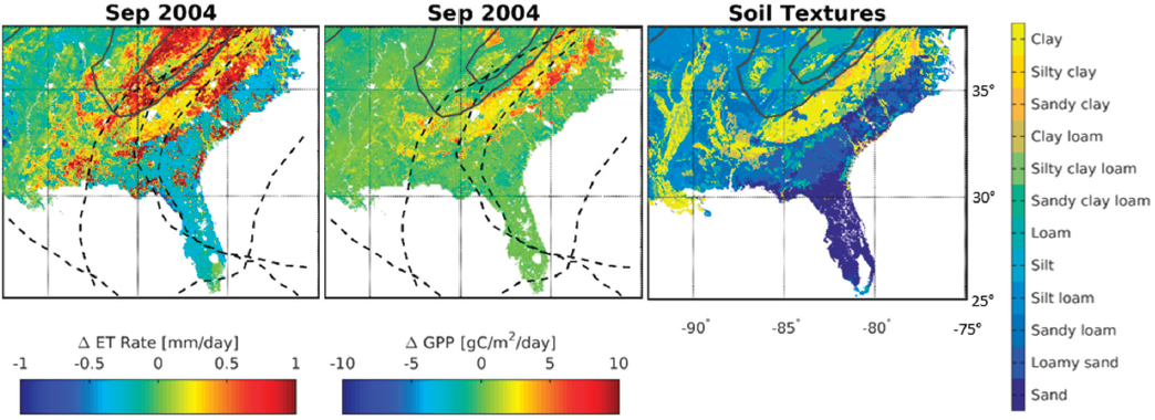
The water and carbon cycles are tightly linked via complex nonlinear feedbacks (Figure 6.7). Vegetation type and condition determine surface radiative properties (e.g., albedo) and root zone soil moisture uptake, and in turn root zone soil moisture availability modulates stomatal conductance, and consequently evapotranspiration (ET), and photosynthesis, and consequently gross primary productivity (GPP). The photosynthesis process governs the metabolism of plants, and it links the loss of vapor from the plant and the gain of carbon for biomass growth from the atmosphere. ET and GPP exhibit large spatial variability with topography, soil type, and land use, as well as large seasonal and interannual variability with precipitation, especially during the warm season (Lowman and Barros, 2016; Yang et al., 2015).
Quantifying evapotranspiration and understanding its linkages is a grand challenge for Earth system science in the coming decade, given the following principles and observations:
- The central role of evapotranspiration in coupling the global water, energy and biogeochemical cycles;
- The importance of the flux to the health and productivity of natural and agricultural ecosystems;
- The already-realized several-fold changes in evapotranspiration through human alterations of the landscape;
- The potential for amplification of these changes under climate change; and
- The paucity, or total lack, of any direct estimates of evapotranspiration regionally and globally.
The rates and spatial patterns continue to change as humans further modify the physical landscape and alter the vegetation cover. To understand their historical change, current state and future outlook, a more complete understanding of the processes that drive variations in these fluxes is essential.
Basic questions include the following:
- How do the rates of evapotranspiration respond to human alterations to the physical landscape and vegetation cover and to shifts in climate and its seasonality? These changes remain as gaps in our knowledge of how the Earth system works. Understanding them is essential if we are to become better stewards of the terrestrial biosphere that we have appropriated so pervasively. Evapotranspiration flux can experience changes that amplify shifts in the precipitation and radiation forcing. Knowledge of changes in their magnitude and regional patterns in the future are critical to understanding the impacts of climate change.
- How does the rate of evapotranspiration respond to changes in precipitation and radiative forcing? These rates are not understood, and they are a source of uncertainty in assessment of climate change impacts (NRC, 2012). Evapotranspiration is a flux at the land-atmosphere interface. Its spatial variations are strongly related to soil type, topography, vegetation, and climate. Their dynamics are affected by the variations in plant growth, weather and seasonal climate. To adequately characterize them, mapping at tens to hundreds of meters and temporal sampling at days to a week are needed at minimum (NRC, 2004). In situ monitoring is not a viable approach for collecting the required data. Observations are needed that span large areas, because installing and maintaining instrumentation at even a single site is costly and challenging (Baldocchi et al., 2001). In this regard, the upcoming ECOSTRESS mission provides a pathway to long-term, spaceborne measurements needed for high-resolution evapotranspiration estimates and to improve the remote sensing algorithms relying on the relationship between land-surface temperature (LST) and evapotranspiration.
Also as a flux, evapotranspiration cannot be directly sensed, as the rates do not uniquely correspond to the thermal or dielectric state of the soil and the vegetation at one level. Rather, they are controlled by vertical and temporal gradients of state variables. Soil moisture is the fundamental state variable that directly controls evapotranspiration (Pollacco and Mohanty, 2012). Vertical gradients in soil moisture drive evapotranspiration and water availability to plant roots. Vertical profiles of soil moisture need to be measured or estimated via integrated models and observations systems (e.g., H-1a) in order to allow estimation of evapotranspiration. SMAP measures soil moisture in the top 5-10 cm and has enabled understanding of links between precipitation, surface soil moisture, and energy fluxes at very coarse spatial scales (10 s km). Information about the top meter of the soil at spatial resolutions that capture the spatial variability in precipitation, energy fluxes, and shallow subsurface flows would enable closing the water budget, including water use by vegetation in the root zone.
Objective H-2b. Quantify the magnitude of anthropogenic processes that cause changes in radiative forcing, temperature, snowmelt, and ice melt, as they alter downstream water quantity and quality.
Snow is the brightest land cover in nature. In the solar spectrum, snow has a distinctive spectral signature—among the brightest natural substances in the visible wavelengths, reduced slightly in the near-infrared beyond 1 µm, and dark beyond about 1.6 µm in the shortwave-infrared—corresponding to the variability in the absorption properties of ice (Warren, 1982; Warren and Brandt, 2008). In the visible wavelengths, both ice and water are transparent to radiation, whereas in the shortwave-infrared both are strongly absorptive. Because snow is so distinctive, mapping of snow-covered areas was one of the first
applications of remote sensing in the hydrologic sciences (Lettenmaier et al., 2015), and the combination of visible and shortwave-infrared bands enables discrimination between snow and clouds (Crane and Anderson, 1984).
Characterization of snow and its rate of melt is critical for understanding the Earth system, and its role in regional hydrology for those river basins where people depend on snow- or glacier-melt for water resources. Snow’s high but variable albedo and low thermal conductivity together sustain stability of the boundary layer over vast regions (Levis et al., 2007). Our understanding of the strength of the simulated snow albedo feedback, however, varies by a factor of three in global climate models (Lemke et al., 2007), mainly attributed to uncertainties in snow extent and the albedo of snow-covered areas from imprecise remote sensing retrievals (Flanner et al., 2009; Fletcher et al., 2009). Snow cover and its melt also dominate regional hydrology over much of the world. Not only does one-fifth of Earth’s population depend on snow- or glacier-melt for water resources, people in these areas generate one-fourth of the global domestic product (Barnett et al., 2005). While long-term observations in many mountain ranges worldwide show a declining snowpack attributable to global warming (Mote et al., 2005; Shekhar et al., 2010), and thus declining glaciers caused by the overlying snow melting earlier in the spring, an equally important anthropogenic contribution lies in the increase in carbonaceous aerosols from combustion and dust from land degradation, darkening the snow and causing its warming due to greater absorption of solar radiation that accelerates melting (Kaspari et al., 2014; Painter et al., 2007; 2013). Earlier snowmelt also warms the climate indirectly by changing terrestrial radiative properties (albedo and emissivity) by earlier exposure of the underlying soil and vegetation. Locally, forest fires yield a source of charcoal that affects snow albedo for many years following the fire (Gleason et al., 2013). Earlier snowmelt affects the seasonal distribution of streamflows, along with the quality of that water, depending on the wet and dry atmospheric deposition of particles and chemicals into the snowpack (Williams and Melack, 1991a, b). Moreover, management of forests implies management of water—for example, in warmer climates, forest thinning retards the rate at which snow disappears (Lundquist et al., 2013).
For these reasons, understanding and managing water from snow- and glacier-dominated basins requires tracking the energy sources that melt the snow and thereby the spatiotemporal distribution of snow and ice properties, especially its albedo as it varies with grain size and presence of absorbing aerosols (Warren, 1982), dust, and rock debris. The same processes govern the health of glaciers that comprise the iconic features of many areas of the world, as they incorporate the history of snowfall during the accumulation season and snow- and ice-melt during the ablation season.
Objective H-2c. Quantify how changes in land use, land cover, and water use related to agricultural activities, food production, and forest management affect water quality and especially groundwater recharge, threatening sustainability of future water supplies.
Agricultural activities involve the conversion of preexisting land uses into pasture or crops, and in many parts of the world, entail managed forest clearing. Most of the heavily irrigated regions were converted from grasslands or from other nonforested systems. Specifically, the impact of conversion of native land to agriculture alters the terrestrial water cycle in both quantity and quality. These changes in the land use and land cover affect infiltration, surface runoff, recharge to the groundwater, water quality, sediment loss, and surface albedo, as well as affecting the temporal dynamics of all of these processes. The water quality variables affected include erosion and sediment loss, total dissolved solids, nitrogen in the forms of nitrate or nitrite, and phosphorus.
Impacts to the hydrologic cycle differ in nonirrigated and irrigated systems. In the nonirrigated, rain-fed case, the water input to the land does not change appreciably except due to weather and climate variabil-
ity and change. Evapotranspiration, however, may increase or decrease due to changes in the vegetation water demand, as well as rising temperatures and wind forcing due to climate change, thereby affecting groundwater levels, and in turn, streams and other groundwater-dependent ecosystems. The changes can be significant but difficult to determine, making unclear the cause-effect links between land use change and water quantity and quality. A particular challenge in rain-fed systems is the difficulty of resolving the precipitation and evapotranspiration sufficiently accurately to estimate groundwater recharge. As in natural ecosystems, the error in evapotranspiration measurements or estimates often exceeds the magnitude of groundwater recharge, a challenge to coupling surface and subsurface hydrologic processes.
Much of the world’s food supply comes from irrigation in dry to moderate climates. Consequently, by far most of the water diverted, impounded, or pumped by humans is for irrigated agriculture (Wada et al., 2013; 2014). Accordingly, irrigated agriculture has created massive dislocations in water stores and disruptions in the hydrologic cycle, as documented by GRACE (Richey et al., 2015), with the record expected to continue with GRACE-Follow On (GRACE-FO). In systems where substantial surface water is available such as California, diversion of surface water for irrigation has caused massive increases in recharge and rising groundwater levels (Faunt et al., 2009; Williamson et al., 1989). In irrigated areas of California where groundwater pumping is not sufficiently high, elevated groundwater levels have caused soil salinity problems akin to those that caused the collapse of agriculture in Mesopotamia by circa 2300 BCE. Conversely, in many other areas of California, excessive, uncontrolled pumping of groundwater has caused groundwater deficits and the attendant undesirable effects, including land subsidence, nonsustainable storage depletion, water quality degradation and increased energy costs (Cannon Leahy, 2016).
The preceding themes, where irrigated agriculture causes either waterlogged soils or nonsustainable groundwater depletion, have been rather common occurrences throughout the world, including the Great Plains and southwestern United States, North China Plain, India, North Africa, South Africa, Australia, and so on. Concomitant with the agricultural water quantity problems are ongoing degradation in groundwater quality owing to salt, nitrate, and other contaminants inherent to agricultural practices. Worldwide, increasing difficulty in sustainably managing water quantity and quality, whether in the subsurface or on the surface, remains a major challenge to soil conservation, food production, and the future of human civilization. This worsening situation calls for combined management of surface water and groundwater that is possible only through advanced, multiscale measurement of all the major water stores and the fluxes between them, with special emphasis on groundwater stores, evapotranspiration, precipitation, recharge, and surface water flows.
While recharge in irrigated regions is reasonably well estimated based on knowledge of crop-water demands, amounts of applied water, and irrigation efficiencies, estimation of recharge in nonirrigated lands is much more challenging. There are several studies on recharge quantification. Scanlon et al. (2006) studied recharge in 140 sites in semiarid and arid regions using the chloride mass balance technique. They found a longer scale variability of recharge rates that depends on El Niño/La Niña and other atmospheric and oceanic variability, and that in relatively warm arid and semiarid regions with thick vadose zones, little or no upland recharge occurs due to native plant adaptation and thermal gradients forcing water vapor upward. Furthermore, regional hydrogeology and the spatial organization of preferential recharge zones and pathways vis-à-vis precipitation patterns play an important role in redistributing groundwater regionally in space and time at multiple scales (Barros et al., 2017). Concentration of runoff in ephemeral channels or areas of high infiltration rates or karstic zones are necessary to overcome thermal gradients and low conductivities and high suctions in unsaturated zone soils (Coes and Pool, 2007; Goodrich et al., 2004; Scott et al., 2000).
Scanlon et al. (2007) carried out a comprehensive study of the impact of agriculture on water resources, both water quality and quantity. In some instances the conversion of native vegetation to croplands could
increase the recharge to the aquifers but degrade the water quality. However, the exact nature of this balance depends on the type of vegetation being replaced. In general conversion to agriculture increases the consumption of water and decreases streamflow and raises the water table and in some regions of the world causes waterlogging. However, groundwater-fed irrigation generally lowers the water table in many parts of the world (Northern India, High Plains and Central Valley United States). As observations for estimation of changes in the terrestrial water cycle owing to conversion of land cover from native to agriculture are limited, there has been a use of models such as the Soil Water Assessment Tool (SWAT) to study this issue (Arnold and Fohrer, 2005), and the Variable Infiltration Capacity (VIC) model has been used in the Great Lakes Region to study the impact of the conversion of forests and prairie grasslands to agriculture (Mao and Cherkauer, 2009). One of the earliest and most influential studies (Allan et al., 1997) emphasized the joint management of land and water and the fact that the two were deeply connected, and that the fractional area of agricultural land within a catchment was the best indicator of streamwater quality (higher sediment and nutrient concentrations) based on a study of the River Raisin Basin in southeastern Michigan using a 20-year (1968-1998) study period. Similar land use impacts have been observed in water chemistry (phosphorus P, nitrogen N, and total dissolved solids TDS) in the Saginaw Bay catchment of Central Michigan (Johnson et al., 1997). Phosphate and nitrate in agricultural fertilizer and TDS are mobilized during storms due to the erosive nature of the rainfall impact, which dislodges the soil, and they end up in surface runoff (Hart et al., 2004; Ahearn et al., 2005), thus linking regional weather and climate, precipitation physics, and water quality.
H-3: Availability of Freshwater and Coupling with Biogeochemical Cycles
Question H-3. How do changes in the water cycle impact local and regional freshwater availability, alter the biotic life of streams, and affect ecosystems and the services these provide?
One of the biggest challenges facing human society is the availability of freshwater where it is needed, when it is needed. In fact, at times there is lack of water (droughts) and yet at other times there is too much water (floods). Global climate change, population and economic growth, land use change, water quality degradation, and aging infrastructure are altering water availability and demand equilibrium at every scale (Sun et al., 2008; Padowski and Jawitz, 2009; Ajami et al., 2014; Hering et al., 2013). Coping with these changes and enhancing adaptive capacity of any region relies on informed and sustainable management of our limited water resources. Access to high-resolution (both spatial and temporal) water quantity and quality data is key in enabling integrated water management and enhancing local human and ecosystem health.
Objective H-3a. Develop methods and systems for monitoring water quality for human health and ecosystem services.
While water availability, environmental and ecosystem health, and social and economic well-being are directly affected by water quantity and quality, current Earth observation missions are not fully equipped to measure the quality of inland water bodies such as lakes, rivers, reservoirs, and estuaries, at an appropriate temporal and spatial scale, and enabling technology is still lacking. In addition, there are many water quality indicators that vary independently while having a combined effect on the remote sensing signals (Ampe et al., 2015). This phenomenon makes the sensing process much more complex and in need of methodologies that could invert gathered signals to effectively infer the accurate information (Chang et al., 2015). In recent years there have been some attempts to infer water quality data and map related environmental and biogeophysical processes using the mosaic of available remotely sensed measurements (Usali and Ismail,
2010; Chang et al., 2015; Fichot et al., 2015; Ampe et al., 2015). However, these are limited in size and scope and they still need in situ data to establish and validate the inference methodology.
To advance water quality sensing from space we need to understand (1) the availability and potential utility of various sensing approaches (visible, infrared, and microwave) and how these technologies can be combined to monitor and measure water and ecosystem dynamics; (2) the temporal and spatial scales governing process dynamics and the measurement resolution needed to inform the decision-making process at the local level; (3) the availability of inversion methodologies that have to be developed to leverage satellite data more effectively; and (4) the cost-benefit analysis of remote-sensing strategies (e.g., drones) alternative to space missions.
Objective H-3b. Monitor and understand the coupled natural and anthropogenic processes that change water quality, fluxes, and storages, in and between all reservoirs (atmosphere, rivers, lakes, groundwater, and glaciers), and the response to extreme events.
In many parts of the world, complete transformation of land cover including deforestation, extensive row crop agriculture, and urbanization are affecting the eco-hydrology at local, regional, and continental scales. Change of fluxes and storages, and the transport and residence times of water in the terrestrial part of the landscape, in the streams, and in the subsurface affect bio-geochemical processes and impact water quality and stream biology. A prime example is the midwestern United States, where intensified row crop agriculture—mainly corn and soybeans providing 40 percent of the global supply—along with drainage of wetlands and the extensive subsurface tile drainage system needed to keep the plant roots dry during the growing season, has increased streamflow volumes and peaks (Guanter et al., 2014), which together with increased precipitation over the past decades (Groisman et al., 2012) have accelerated near-bank erosion, and increased nutrient loads contributing to the Gulf of Mexico hypoxia (Blann et al., 2009; Belmont et al., 2011; Novotny and Stefan, 2007; Schilling et al., 2010; Zhang and Schilling, 2006; Foufoula-Georgiou et al., 2015). Similar changes are observed in coastal areas where climatic and human impacts (e.g., sea-level rise and local and upstream basin development that reduce water and sediment to the coast, accelerating subsidence) contribute to increased saltwater intrusion, coastal erosion, degradation of protective vegetation and marshes, and decline of unique biodiversity (Ericson et al., 2006; Syvitski et al., 2009; Tessler et al., 2015).
Remote sensing observations of multiple coupled variables are needed therefore to achieve Objective H-3b (e.g., rainfall, soil moisture, photosynthesis, sediment/water interfaces, river migration rates, water stages, and vegetation composition) at spatial and temporal scales appropriate for detection of trends, local predictive modeling, and mitigation actions on the ground including urban expansion, deforestation, and agricultural practices. Collecting such comprehensive data sets, which is prohibitive on the ground, is necessary to understand and model the coupled human-natural system in an integrated Earth systems modeling perspective. Of special interest is the effect of extremes on the eco-hydrologic trajectories of landscapes at seasonal, annual, and multidecadal time scales and implications for global water cycling, landscape connectivity, and carbon storage.
Objective H-3c. Determine structure, productivity, and health of plants to constrain estimates of evapotranspiration.
The components of evapotranspiration include (1) transpiration from plants; (2) rain or snow intercepted by the plant canopy that subsequently evaporates or sublimates; and (3) evaporation from the soil surface. Plant species, structure (individual and within a complex stand with understory), leaf area, and stomatal
density all affect transpiration and interception. Improved knowledge of plant structure and its change over time (productivity and health) will therefore translate directly into improved estimates of evapotranspiration. Spectral remote sensing and associated retrieval methods have proven successful in identifying monoculture or spatially dominant plant species with automatic and supervised classification algorithms. Likewise, numerous vegetation indices have been developed to successfully identify plant chlorophyll, photosynthetically active vegetation, plant vigor, and the phenological cycles of annual and deciduous plant species (Huete et al., 2002).
Spectral methods have had less success in complex multispecies stands where overstory shading, interwoven branches, and understory plants are present. In these instances leaf area index (LAI) and surface roughness affecting canopy conductance are not well estimated (Dingman, 2014). Even within a monoculture stand, the LAI of some species such as cottonwood (Populus fremontii) cannot be accurately estimated with spectral remote sensing, and allometric relationships change with tree age (Farid et al., 2006).
Multireturn and waveform lidar can address many of the shortcomings of spectral-based remote sensing noted earlier. Lidar employs a laser system on a platform that transmits laser pulses toward any object of interest at rates up to hundreds of thousands per second. The laser energy interacts with the object (e.g., vegetation, terrain, and structures), and some of the energy is reflected back toward the lidar receiver. If the position and orientation of the moving or stationary lidar instrument platform is known in time and space, the x, y, and z coordinates and return intensity of the reflected portion of the laser pulse can be determined. Airborne, spaceborne, mobile, drone-based, and terrestrial laser scanning systems are advancing rapidly (Jensen, 2006; Lefsky et al., 2002). One National Research Council study concluded (NRC, 2007b) that lidar should be acquired over the entire continental United States based solely on the benefits to improved flood plain mapping for the Federal Emergency Management Agency (FEMA) Map Modernization program.
Lidar has been used extensively for forest inventory and structure (Lim et al., 2003), biomass and carbon stocks (Asner et al., 2012), estimation of LAI (Korhonen et al., 2011), and to constrain and improve evapotranspiration estimates (Farid et al., 2008; Mitchell et al., 2012). More recently, single-photon and Geiger lidar are being employed in nondefense applications. These new systems split a single laser pulse into numerous subpulses, which are then detected with segmented detectors. They offer higher effective pulse rates (~200 million samples per second) over linear-mode lidar (~500,000 samples per second) with lower power needs (1-2 W for single photo and 20-40 W for Geiger) (Jasinski et al., 2016). A single-photon lidar device is being deployed on the upcoming 2017 ICESat-2 mission in the Advanced Topographic Laser Altimeter System (ATLAS) instrument, with the primary goal of polar ice sheet thickness measurements (Abdalati et al., 2010). ATLAS will employ one laser split into six beams at roughly 10,000 pulses per second.
If advances in lidar technology can continue apace so that within 10 to 15 years, spaceborne platforms can provide the 20 to 30 return points per square meter that airborne platforms currently provide, a rich set of attributes on vegetation structure and productivity could be derived to constrain and improve evapotranspiration estimates. The additional benefits of these data to hydrology include improved topography for flow path and drainage derivations, surface water levels, snow depths, and near shore bathometry. Benefits to other disciplines would also be numerous, including landslide characterization, postfire erosion, and postfire recovery for hazards; carbon inventories for ecosystems; and ice volumes and depths for solid Earth.
H-4: Hazards, Extremes, and Sea-Level Rise
Question H-4. How does the water cycle interact with other Earth system processes to change the predictability and impacts of hazardous events and hazard chains (e.g., floods, wildfires, landslides, coastal
loss, subsidence, droughts, human health, and ecosystem health), and how do we improve preparedness and mitigation of water-related extreme events?
Objective H-4a. Monitor and understand hazard response in rugged terrain and land margins to heavy rainfall, temperature and evaporation extremes, and strong winds at multiple temporal and spatial scales.
This socioeconomic priority depends on the success of addressing Objectives H-1b, H-1c, H-2a, and H-2c. Natural disasters pose major threats to the livelihood and security of millions of people worldwide. Increasing trends of natural disaster impacts can be linked to amplification of the hydrologic cycle from climate-related events (Field et al., 2012), dramatic changes in land use and land degradation, and overpopulation in at-risk areas (e.g., coastlines, river margins, estuaries and deltas, mountainous regions) (Oki and Kanae, 2006). Recent estimates indicate that over 88 percent of natural disasters are water related (Adikari and Yoshitani, 2009) and are one of the greatest global threats to socioeconomic development. Depending on the nature and location of the event, the number of people affected by natural hazards can range from hundreds to thousands (e.g., landslides), to several million (e.g., regional flooding and agricultural drought). Lasting impacts of natural hazards include significant damage to infrastructure, land degradation, loss of life, economic loss, disease, and combinations thereof.
Sustainable risk reduction of natural hazards consists of prevention and preparation as well as mitigation and response. Thus, it requires not only proper characterization and understanding of the events themselves, but also sufficient modeling and prediction of the processes that underlie and drive the hazards. Given the nature of water-related disasters, impacts from too much or too little water can result in a wide array of events, including coastal and lake floods, flash floods, hurricanes, landslides and avalanches, subsidence, agricultural droughts, and waterborne epidemics. A key question to understanding these events is: How does the water cycle interact with other Earth system processes to change the probabilities, magnitudes, and frequency of these events? To this end, improved understanding of the quantification of their dynamics and impacts is needed.
Hazard process monitoring and modeling in at-risk areas such as mountainous terrain and land margins such as coastlines, floodplains, deltas and estuaries, and land-water interfaces generally is particularly needed. Some key measurement variables common to these Earth system process and water-related hazards include precipitation, soil moisture, snowmelt, water depth, water flow, and atmospheric water vapor (for monitoring and predicting certain weather conditions). The ability to measure these variables at the temporal and spatial scales consistent with event dynamics is crucial for improved hazard response. For example, severe thunderstorms can be on a local (1-10 km) spatial scale and can evolve in a matter of minutes (Schmidt et al., 2009; Mathew et al., 2014). On the other hand, several slow-onset drought events have occurred in the past decade (AghaKouchak et al., 2014; Long et al., 2013), with magnitudes and intensities leading to regional and long-standing (months to years) impacts.
Several applications of Earth observations exist for improved hazard mitigation. In mountainous regions, frequent measurements of near-surface soil moisture and of snow water equivalent (SWE) coupled with physically based models can improve landslide susceptibility mapping by estimating antecedent soil moisture conditions and snowmelt and isolating the triggers for the onset of spring season landslides. Regular monitoring of streamflow can enable improved management of risk and water strategies in flood-prone areas. Evapotranspiration has been shown to be a critical hydrologic variable for capturing drought magnitude, intensity, and timing (Anderson et al., 2011; Fisher, 2014). At low elevations, along the land margins of the world’s major rivers and coastlines, surface water elevation measurements from the Surface Water and Ocean Topography (SWOT) mission can potentially improve inundation mapping as well as serve as boundary conditions for high-resolution models of rivers, storm surges, and coastal circulation.
In addition to providing increased hazard security and forecasting, key questions to be addressed by the implementation of Earth observations needed for monitoring and modeling hazard response include the following:
- How are changes in land use affecting evapotranspiration rates, and how do these in turn affect local and regional precipitation systems, temperature extremes, and carbon cycling?
- How does the water cycle interact with other Earth system processes to change the probabilities and impacts of hazardous events and hazard chains such as floods, wildfires, landslides, coastal loss, subsidence, droughts, and human and ecosystem health?
- How do we improve preparedness and mitigation of water-related extreme events using measurements and integrated observing systems and models?
- Can we improve our understanding of trigger mechanisms to improve predictions for all hazards and flooding and landslides—in particular, in headwater basins and along land margins?
- How do we improve our understanding of post-hazard landscape response using integrated systems and models toward more effective recovery and preparedness?
Objective H-4b. Quantify key meteorological, glaciological, and solid Earth dynamical and state variables and processes controlling flash floods and rapid hazard chains to improve detection, prediction, and preparedness.
This socioeconomic priority depends on the success of addressing Objectives H-1b, H-1c, and H-4a. Floods and other hazards, like landslides, can devastate communities. In 1999, combined flash floods and landslides claimed the lives of 30,000 Venezuelans, displaced an additional 110,000 residents, and destroyed 23,200 homes (IFRC, 2000). In July of 2012, a 7 m wall of water raced through the town of Krymsk in southern Russia, killing 170 people and displacing 13,000 (Russia Today, 2012). Increased risk of persistent and intermittent inundation due to increased runoff in flat terrain is linked to increased storm activity, sea-level rise, and storm surges, within the context of coastal landscapes hardened by built infrastructure; the resulting increased risk of persistent and intermittent inundation poses a significant societal challenge (Tebaldi et al., 2012; Hallegatte et al., 2013).
Figure 6.8 shows how predicted sea-level rise interacts with storms to increase the probability of catastrophic coastal floods in Boston. In the United States, the 2015 damages from flash floods reached $2.1 billion, with 129 deaths (NOAA, 2015). While other flooding hazards have a broad impact on U.S. society, flash floods are the ones that consistently kill more people (Ashley and Ashley, 2008). Figure 6.9 provides a synopsis of reported flashflood occurrences over a 5-year period in the continental United States. Rainfall-induced landslides are equally destructive. The U.S. Geological Survey (USGS) estimates that the annual cost of landslides in the United States is between $2 billion to $4 billion and that 25 to 50 people are killed by them (USGS, 2016). Worldwide, between the years 2004 and 2010, 2620 deadly landslides killed 32,000 people (Petley, 2012); though not all were rainfall induced, the great majority were.
Flash floods and shallow, rainfall-induced landslides are caused by high-intensity, high-volume precipitation events coupled with the proper hydrological scenario, which is defined by current soil moisture; the slope, shape, and soil types of the basin; the impervious region in the basin; and the built drainage structures of the basin. As our climate warms, the hydrologic cycle is shifting toward an overall increase in heavy precipitation events across the United States (2005; Groisman et al., 2004). The risk of and impact of flash floods and landslides increases with the frequency of intense or long-duration precipitation.
Figure 6.10 shows the global distribution of landslide occurrences overlying a global landslide susceptibility map (Kirschbaum et al., 2009). Because both hazards depend on precipitation and the physiographic
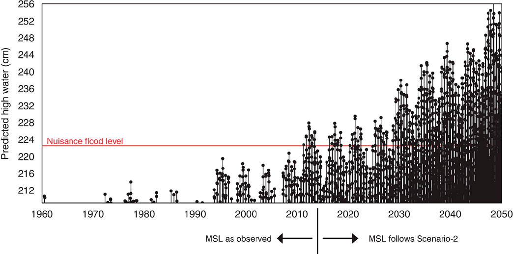
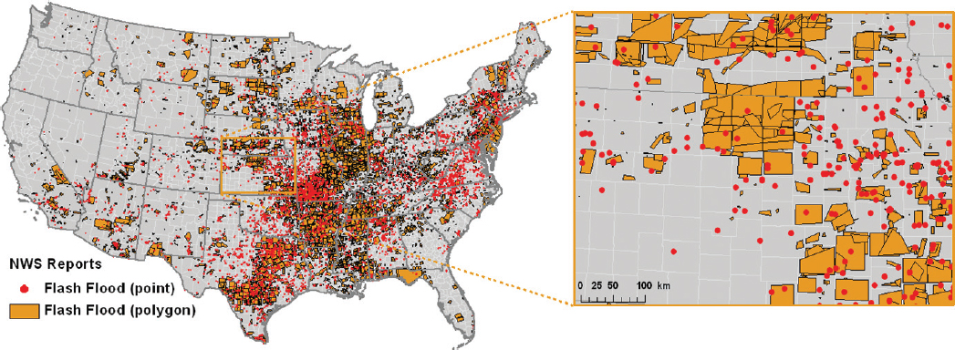
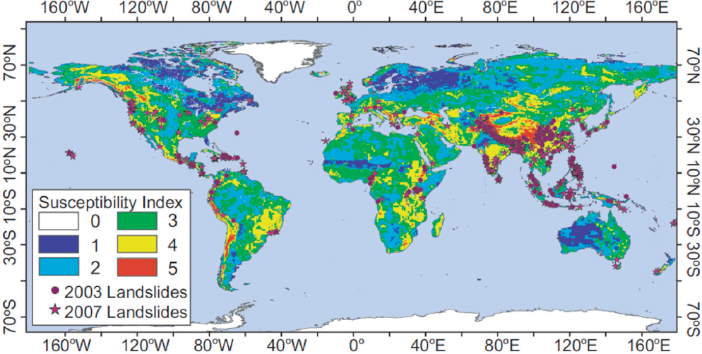
characteristics of a region, both offer the possibility of mitigation through Early Warning Systems based on observed and forecast precipitation intensity coupled with a model of regional topography, geology, and land use and land cover (Gourley et al., 2011; Hong et al., 2007; Hossain, 2006; Sättele et al., 2015). Although uncertainty in estimating precipitation intensity in mountainous regions, as well as ambiguity with regard to the definition of susceptibility index classes, pose challenges to forecast skill, this methodology was used to increase situational awareness to the U.S. Army and its partners during the Peruvian floods and landslides in 2015-2016 linked to a strong El Niño. NASA Global Precipitation Measurement (GPM) satellite precipitation estimates are already being used for flood and landslide nowcasting purposes and to quantify risk (Kirschbaum et al., 2015; Stanley and Kirschbaum, 2017; Wu et al., 2014). Further, these models can be coupled to hyper-resolution physically based models to pinpoint hotspots of slope instability and warnings (Tao and Barros, 2014b).
While an Early Warning System cannot stop a 7 m wall of water from descending upon a city, an Early Warning System can provide the lead time necessary for people to move out of harm’s way. As noted by Di Baldassarre et al. (2010), Early Warning Systems were critical in reducing the impacts of floods in India and the Czech Republic. An effective Early Warning System depends on informative input data and a model that uses that data to project into the future. Improving the predictability of the flashy events will depend on improving the measurements of the input data as well as improving our understanding of the processes that control these phenomena and so improve our predictive models. Near-real-time (i.e., latency depends on telecommunications or post-processing) monitoring—such as the WMO Global Telecommunications System (WMO, 2017), the Global Flood Monitoring System (GFMS, 2017), the Dartmouth Flood Observatory (DFO, 2017), and the Global Flood Detection System, part of the Global Disaster Alert and
Coordination System (GDACS, 2017)—can update initial conditions and identify “Early Watch Regions” to which modeling efforts can be directed aiming at improving forecast lead times and situational awareness. Predictions and early warnings in mountainous regions remain the most challenging due to the difficulties of precipitation retrieval in complex terrain and the very rapid rainfall-runoff response in steep terrain. Tao and Barros, (2013) showed that by merging GPM-like observations with Quantitative Precipitation Forecasts (QPFs) from the National Forecast Database (NDFD), significant improvements (up to 50 percent) could be attained in the skill of Quantitative Flood Forecasts (QFFs) using physically based models, as long as revisit time is less than the response time of specific watersheds. Further, significant inroads toward longer warning lead times can be expected through coupled prediction frameworks and data assimilation systems to integrate forecasts and observations (Tao et al., 2016). Indeed, systems such as NOAA’s Rapid Refresh (Benjamin et al., 2015) with assimilation of ground-based radar data every 15 minutes at present can be envisioned only for operations outside the continental United States by assimilating remote-sensing observations (e.g., satellite-based radar, as discussed in the section on Objective H-1b). Analysis of large observational data sets provides unique opportunities for developing targeted location-specific flood and debris flow forecasts with lead times of hours to days (Akhtar et al., 2009; Campolo et al., 2003; Kim and Barros, 2001; Sättele et al., 2015).
In many glacierized mountains, and Arctic lowland countries with glaciers, glacier thinning and retreat are causing the growth of glacial lakes. Glacier lake outburst floods are an important natural hazard in many of these places, such as Alaska, Greenland, Iceland, Peru, and Nepal (Bajracharya et al., 2007). Debris flows, ice and snow avalanches, landslides, and—on ice-capped volcanoes—lahars are frequent and sometimes deadly consequences of heavy precipitation and snow and ice accumulation on steep slopes. The interactions between the solid Earth and land cover and surface dynamics—for example, earthquake triggering of ice avalanches and landslides, landslide blocking of rivers, and consequent landslide-dammed lake outburst floods—can be strongly influenced by the preceding history of the thermal state and retreat of glaciers, or by the seasonal state of shallow groundwater saturation of soils and snow melting (Kargel et al., 2016).
Economically vital minerals and petroleum and gas extraction and transport from and through mountains and over lowland areas of permafrost and beside or across rivers, the routing pipelines, roads, and bridges, and the security of mountain villages and cities must consider the multitude of hazards due to rainfall runoff floods, snowmelt floods, glacier lake outburst floods, thawing permafrost, as well as glacier surges, landslides, snow and ice avalanches, and other physical elements and processes of the hydrogeological environment. The mountain hazard environment is changing around the world due to climate change as glaciers thin and retreat, snowpack and monsoonal precipitation patterns change, patterns and intensity of freeze-thaw processes shift, and vegetation communities are altered. Likewise, coastal hydrology in relation to rivers and lake and seacoasts is manifestly altered by the effects of climate change, floods, and land subsidence and uplift and general sea-level rise. The tracking of hydrologic and hydrogeological natural hazards requires optical and radar methods of monitoring changes to glaciers and glacier lakes, snowpack, rivers, lakes, and vegetation; thermal monitoring of volcanoes; and high-resolution topographic mapping. The large data sets produced by satellite monitoring argue in favor of reliable semiautomated and autonomous hazard detection and monitoring, hazard susceptibility mapping, and hazard forecasting and real-time warnings (Kirschbaum et al., 2016), along with development of reliable human networks to support uniform, standardized data analysis.
Because much of the world is not well instrumented, including many areas that are vulnerable to these high-impact episodic hazards, spaceborne, remotely sensed data are needed to provide the precipitation and antecedent conditions. As with other Hydrology Panel priorities, the measurement of worldwide precipitation, Objective H-1b, will be essential to enhancing our ability to predict flash floods and landslides.
The characterization of the antecedent conditions, both the fixed topographic variables and the dynamic variables like soil moisture, plant growth, and current river stage, will also be required, as is the case with Objectives H-3a, H-3b, H-4a, and H-4b. Good measurements need to be integrated into models to forecast the likely future precipitation and then the resulting surface processes that may (or may not) result in a flash flood or landslide.
Objective H-4c. Improve drought monitoring to forecast short-term impacts more accurately and to assess potential mitigations.
This socioeconomic priority depends on the success of addressing Objectives H-1b, H-1c, and H-2c. Droughts have significant economic and societal impacts. Unlike other extremes, their onset tends to be slow, their persistence long, and their recovery poorly predicted. Wilhite, (2000) estimated the average annual drought impact in the United States at $6 billion to $8 billion, while the 2015 severe drought in California was estimated to have $2.7 billion in damages in the agricultural sector alone (Howitt et al., 2015).
Compared to other natural disasters, a greater proportion of the population can be affected by droughts. Although droughts can have larger impacts on gross national products in the more developed countries, the magnitude of impacts on people’s health and overall well-being is especially severe in less-developed regions. In Africa, droughts account for less than 20 percent of natural disasters but account for over 80 percent of the affected population (UNISDR, 2009). It is estimated that 300,000 people died in Ethiopia alone during the height of the Sahel drought in the early 1980s (EM-DAT, 2017) due to crop failure, lack of drinking water, and disease. Half a million people are estimated to have died because of drought-related impacts in Africa during the 1980s (Kallis, 2008). The impacts of drought are intimately linked to the vulnerability of a population to adverse conditions and how society responds within the constraints of changing economies. In general, loss of life is greater in developing regions, and the economic impacts are greater in the developed world. Timely determination from a drought early warning system and monitoring drought will aid the decision-making process in order to reduce drought impacts (Wilhite et al., 2007).
Drought is defined as a deficit (relative to an appropriately defined normal) of water in one or a combination of water stores (river, lake, reservoir, snowpack, soil water, or groundwater) or water fluxes (precipitation, evapotranspiration, or runoff). Depending on the water deficit, drought is usually classified as (1) meteorological (a negative departure from mean precipitation); (2) hydrological (a deficit in the supply of surface and subsurface water); or (3) agricultural (a deficit in soil moisture driven by a combination of meteorological and hydrological drought resulting in reduced supply of moisture for plants and crops). A variety of drought indices have been developed to reflect the various types of drought (Sheffield and Wood, 2011).
Observations of hydrologic variables needed to estimate drought indices are scarce over large spatial regions that are of interest for drought monitoring and management, especially in the developing world. Precipitation is one of the best observed variables although near-real-time gauge observations are limited in most regions outside the United States, and gauge networks are also sparse over much of the developing world (e.g., Africa). In situ soil moisture is one of the least observed aspects of the hydrologic cycle in terms of long-term, large-scale measurements. Thus, to overcome the deficiencies in in situ observation systems, remote sensing of precipitation (both liquid and solid) as well as soil moisture is necessary for early warning drought monitoring.
For meteorological drought, progress must be made on addressing Objective H-1b—namely, the improved monitoring of precipitation—and gaining knowledge on the predictability of rainfall at seasonal time scales. For many regions of the globe, winter snow provides the needed water supplies in the summer seasons. Thus, advances in the monitoring of mountain snowpacks, as quantified in Objective
H-1c, is required to make progress on predicting drought in snow-dominated water supply systems. Better monitoring of snowpacks and precipitation, when used with appropriate land-surface models, can help improve river flow predictions, and therefore hydrological drought. Improved predictions of inflows into water supply reservoirs are a key requirement for early warning and planning of such hydrological droughts.
For agricultural drought, soil moisture is the monitoring variable. There are currently four systems that provide soil moisture products at various spatial and temporal resolutions: MetOp with the advanced scatterometer (ASCAT) (Brocca et al., 2011; Wagner et al., 2013); JAXA’s Advanced Microwave Scanning Radiometer 2 (AMSR2) with the C- and X-band passive radiometers on the GCOM-W1 satellite; ESA’s Soil Moisture and Ocean Salinity (SMOS) L-band radiometer (Kerr et al., 2016); and NASA’s Soil Moisture Active-Passive (SMAP) L-band radiometer and radar (Entekhabi et al., 2010). The preferred system is based on low-frequency microwave active and passive remote sensing where the radiometer provides measurements with high sensitivity but at low resolution and the radar provides high-resolution complementary capability. Airborne experiments have demonstrated that P-band measurements can provide potentially the basis for subsurface sensing of soil moisture in the root zone.
Objective H-4d. Understand linkages between anthropogenic modification of the land, including fire suppression, land use, and urbanization on frequency of and response to hazards.
This objective is linked to Objectives H-2a, H-2b, H-4a, H-4b, and H-4c. Humans have altered landscapes for centuries through development of the built environment, conversion of woodlands to agricultural lands, and more recently, through extensive forest management policies. Conversion of Earth’s surfaces to alternative or highly structured land cover significantly alters land-atmosphere processes, and ultimately, can increase the risk of hazards to human populations. Fire suppression has been a significant goal of forest management policies since the 1920s, facilitating an increase in large wildfires across the western United States (Westerling et al., 2006). Warmer spring and summer temperatures, coupled with lower than average precipitation, have also produced longer wildfire seasons with more frequent and larger fires (Morgan et al., 2008; Westerling et al., 2011). Climate change is also expected to increase fire risk and may lead to changes in vegetation types and increased fuel loads (Spracklen et al., 2009; McKenzie and Littell, 2017). Wildfires impact water resources that are in high demand in the arid West. The acute loss of vegetation reduces infiltration and enhances soil water repellency and decreases soil cohesion and organic matter (Robichaud, 2000; DeBano, 2000), ultimately increasing runoff and the risk of flooding, excessive erosion, and debris flows (Rulli and Rosso, 2007; Ebel et al., 2012). Kinoshita and Hogue, (2011) documented elevated streamflow for 7 years after fire in southern California, while dry season flow increased for over a decade (Kinoshita and Hogue, 2015). Wildfires also impact water quality and threaten drinking water supplies (Smith et al., 2011; Stein et al., 2012; Burke et al., 2013). Nutrients associated with sediments (i.e., total phosphorous) increase in streams impacted by fire (Mast and Clow, 2008; Emelko et al., 2015). Studies on forest fires throughout the western United States and Canadian Rockies also show increases in nitrate concentrations in receiving waters after forest fire (Riggan et al., 1994; Earl and Blinn, 2003; Rhoades et al., 2011; Bladon et al., 2008).
Fire suppression policies, in conjunction with ongoing drought, have also caused extensive insect invasions in North America (Adams et al., 2012; Anderegg et al., 2013; Williams et al., 2010). The mountain pine beetle epidemic has affected conifer forests at historic levels (Raffa et al., 2008), with over 6 million hectares of forests in the United States and British Columbia impacted by bark beetles and more than 5 million ha affected by the mountain pine beetle (Meddens et al., 2012). This includes headwater catchments to the Colorado, Arkansas, Rio Grande, and Missouri Rivers. The progressive reduction in forest canopy due to bark beetle outbreaks does not completely remove the understory vegetation and canopy, making it challenging to predict the impact of bark beetle infestation on watersheds (Mikkelson et al., 2013; Adams
et al., 2012). Recent work (Slinski et al., 2016) for 33 western U.S. watersheds noted no significant change in peak flows or average daily streamflow following bark beetle infestations, and that climate is a stronger driver of streamflow patterns and snowmelt timing than insect forest disturbance for the studied systems.
Biederman et al. (2015) also found a muted hydrologic response in eight infested catchments in the Colorado River headwater to beetle-induced tree die-off. Expectations of increased streamflow were not supported by observations. They attribute the findings to “increased transpiration by surviving vegetation and the growing body of literature documenting increased snow sublimation and evaporation from the subcanopy following die-off in water-limited, snow-dominated forests.”
Urbanization, or the addition of impervious land cover and related infrastructure, has some of the most significant impacts on land-surface processes: increased runoff, decreased lag time between precipitation and runoff (Guan et al., 2016), and larger peak flows (Sheng and Wilson, 2009). This leads to an increase in the risk of flooding in highly urbanized areas and therefore nonstationarity in flood statistics (Cuo et al., 2009; Meierdiercks et al., 2010; Barros et al., 2014), increase in the heat island effect (Rizwan et al., 2008), decreased recharge of groundwater (Harbor, 1994; Rose and Peters, 2001), but increased groundwater recharge in the southwestern United States due to the increases of flow and its concentration in ephemeral channels noted under Objective H-2c (Kennedy et al., 2013), and development of extensive regional infrastructure to transport needed water to urban centers (Mitchell et al., 2001, 2003; White and Greer, 2006). Climate change is also altering regional precipitation and temperature patterns, increasing the risk of extreme events and urban flooding (Ekström et al., 2005; Berggren et al., 2012).
Key needs in space-based estimates for land cover/land use change include higher resolution soil moisture, including at scales for better estimates of plant water availability for evapotranspiration (i.e., less than 1 km and at a daily scale); estimates of plant biomass and density from microwave and visible/near-infrared sensors, including identification of plant type or species for which an imaging spectrometer would benefit; improved estimates of photosynthesis activity (infrared bands to determine plant activity and dynamics); and finer spatial resolution radiation terms, including skin and air temperature, both under clear sky and cloudy conditions. Other critical needs include precipitation at high spatial and temporal resolutions, and lidar for urban and plant structure and form.
Enabling Measurements
This section explains how the objectives described in the previous section translate into measurements. Some measurements are already available from sensors in the Program of Record (Appendix A; already employed or those in the queue). Some require new approaches to the interpretation of existing sensors. Last, this section identifies new measurements that are needed to achieve the objective and describes technologies that might enable them.
In general, the science and applications objectives and the measurements are interrelated, without a one-to-one mapping between them. Many of the lower-priority objectives would be achieved simply as a result of achieving specific higher priority objectives.
To illustrate these relationships, consider Objective H-1a, designated Most Important in Table 6.1 and described as follows: “Develop and evaluate an integrated Earth system analysis with sufficient observational input to accurately quantify the components of the water and energy cycles and their interactions, and to close the water balance from headwater catchments to continental-scale river basins.” Fulfilling this objective requires success with Objectives H-1b and H-1c, and it also requires that we estimate evapotranspiration, which in turn requires that we estimate the surface energy balance, especially the surface radiative fluxes, so surface albedo and temperature are needed. To estimate water availability, we need to know about the soil moisture in the root zone, as well as the vapor pressure deficit between the leaves and
the atmosphere. Last, we gain additional information from knowing the species of the vegetation involved, and the vegetation structure. Table 6.3 maps the Most Important and Very Important objectives from Table 6.1 to measurements and potential technologies for achieving them, including use of sensors already in the Program of Record as well as potential new sensors. Notably, adding the Very Important objectives adds just one set of measurements, related to groundwater, beyond the set of measurements needed to achieve the Most Important objectives. Table 6.4 provides the same information for the Important objectives, in less detail but illustrating that most of those objectives could be achieved if the Most Important and Very Important objectives were addressed.
Details on the measurements, their role in achieving the objectives, and prospects for those measurements are given in the following sections. Some information about current capabilities is extracted from a recent review (Lettenmaier et al., 2015).
Energy and Water Fluxes in the Surface Layer
Radiative Flux at Surface, Downscaled to Topography
Estimating the net solar and net longwave radiation at the surface, corrected for atmospheric attenuation, is crucial for calculating energy-driven water fluxes such as evapotranspiration or snowmelt. While the net radiative fluxes depend on the surface albedo and temperature, they are also driven by the incoming values of solar and longwave radiation, which are affected by the atmosphere and topography. A probing scientific question about Earth’s climate is the net radiation balance of the Earth system. For the hydrologic cycle, the concern mainly addresses the disposition of net radiation at the surface.
At spatial scales of 100 km or so, and especially when averaged over time and space, the surface and top-of-atmosphere estimates of solar and longwave radiation from the Cloud-Earth Radiant Energy System (CERES) instruments on three satellites—Terra, Aqua, and TRMM—are generally viewed as satisfactory (Kato et al., 2011). For hydrologic analyses, however, the same values at temporal intervals for models and at spatial resolutions that reflect topographic variability are needed. In this case the estimates of solar radiation at the surface match station observations on average (Hinkelman et al., 2015), but in the mountains the average atmospheric properties of a CERES grid cell (~1 degree) are often different than at specific locations, especially higher elevations where errors of several hundred W/m2 can occur when clouds are present but not recognized by the sensor (Bair et al., 2016). Longwave radiation estimates are not as easily validated because in situ measurements are less available. Given estimates of incoming direct and diffuse solar radiation, longwave radiation, surface albedo, vegetation structure, and surface temperature, the net values at the surface can be estimated (Rittger et al., 2016).
Probably, atmospheric properties can be downscaled from the CERES resolution using observations from the Program of Record, but this remains a problem to solve. Information about topography is available worldwide from the Shuttle Radar Topography Mission (Farr et al., 2007). Information derived from Landsat imagery for the United States is available via the LANDFIRE product (Rollins, 2009), which could be processed worldwide in the future.
Albedo of Vegetation, Soil, and Snow
Estimation of energy fluxes such as evapotranspiration or snowmelt at the surface requires that we consider the radiative properties of the vegetation, soil, and snow including emissivity and albedo. Albedo is especially critical because it determines the magnitude of the net solar radiation term in the energy budget equations, and because it exhibits spatial, seasonal, and diurnal variability because of changes in local environmental conditions, and with illumination angle (Tao and Barros, 2014a; Bair et al., 2017).
TABLE 6.3 Mapping Most Important and Very Important Objectives in Table 6.1 to Fluxes and State Variables, and Potential Implementations
| Objective | Knowledge Needed | Flux or State Variable (Priority Order) | Potential Technologies |
|---|---|---|---|
| H-1a (MI) | Energy and water fluxes in the surface layer, specifically evapotranspiration, which is not directly measured but instead inferred from the energy fluxes to get the latent heat flux | Radiative flux at surface, downscaled to topography | improved algorithms with existing sensors in the Program of Record: CERES, MODIS, VIIRS, GOES-16, Himawari, MSG |
| Albedo (vegetation and soil, separately) | Imaging spectrometer | ||
| Soil moisture in root zone | L-band and P-band radiometer and radar | ||
| Diurnal cycle of surface temperature (vegetation, soil, snow), at agricultural or topographic scales | Thermal infrared, in 4 µm and 11 µm spectral regions, multiple platforms to get diurnal cycle | ||
| Vapor pressure deficit in boundary layer | Microwave and IR sounders | ||
| Winds in boundary layer | Active sounders, radar or lidar | ||
| Vegetation species | Imaging spectrometer | ||
| Vegetation structure | Landsat (e.g., LandFire extended globally), lidar | ||
| H-1b (MI) | Rainfall | Rain rate at both high and low intensities | Passive and active microwave observations at finer spatial resolutions Geostationary IR/VIS observations to support operational applications (GOES series) |
| Snowfall | Intensity of snowfall and mixed-phase precipitation | Higher frequency radar and radiometer | |
| H-1c (MI) | Snow water equivalent (SWE) | Snow depth, weekly, at topographic scale | Ka-band or lidar altimeter |
| Snow density (less heterogeneous than depth) | Interferometric L-band or S-band SAR or model | ||
| Snowmelt rate | Radiative flux, albedo of snow separately from vegetation and soil, and surface temperature of the snow, at topographic scale | Imaging spectrometer | |
| Sublimation from snow | Thermal infrared, in 4 µm and 11 µm spectral regions, multiple platforms to get diurnal cycle | ||
| H-2a (VI) | Evapotranspiration (ET) | Same as for H-1a, earlier | |
| Land use and land cover | Land use and land cover categories | Landsat and Sentinel-2, in Program of Record | |
| Rainfall | Same as for H-1b, earlier | ||
| H-2c (MI) | Groundwater storage and recharge | Groundwater storage, at basin scale (50 km or better) | Gravimetric measurements if possible to achieve 50 km resolution |
| Interferometric SAR or GPS to measure elastic changes | |||
| Rate of recharge (precipitation-evapotranspiration to accuracy finer than rate of recharge) | See H-1a and H-1b, earlier | ||
| Rate of subsidence (to diagnose overdrafting) | Interferometric L-band or S-band SAR | ||
| H-4a (VI) | Hazard response to extremes | Same as H-1b, H-1c, H-2a, H-2c, earlier |
NOTE: New measurements are indicated in italics.
TABLE 6.4 Mapping Important Objectives in Table 6.1, in Less Detail than in Table 6.3, to Fluxes and State Variables, and Potential Implementations
| Objective | Knowledge Needed | Flux or State Variable (Priority Order) | Potential Technologies |
|---|---|---|---|
| H-2b | Snowmelt | Same as H-1c in Table 6.3 | |
| Water quality | See H-3a, later | ||
| H-3a H-3b |
Water quality | Important biological, chemical, and physical variables (biggest connection between environment and human health) | Something like Pre-Aerosol, Clouds, and Ocean Ecosystem (PACE) at scale of rivers is too expensive, but imaging spectrometer would address many problems |
| H-3c | Structure of vegetation | Leaf and woody variables (need to address which properties are essential to constrain evapotranspiration) | Landsat, imaging spectrometer, lidar |
| H-4b | Flash floods | Same as H-1b, H-1c, H-4a | |
| H-4c | Drought monitoring | Same as H-1b, H-1c, H-2c | |
| H-4d | Linkage between land modification and hazards | Same as H-2a, H-2b, H-4a, H-4b, H-4c | |
NOTE: New measurements are indicated in italics.
Broadband albedo of a surface is the convolution of the spectral albedo with the spectral distribution of solar radiation at the surface. The albedo of an arbitrary land cover cannot be directly measured with a multispectral sensor. Even if the atmospheric attenuation of the signal is corrected, estimating the albedo requires interpolating between the wavelengths where the reflected radiance is measured. Moreover, calculation of evapotranspiration or snowmelt might require the albedo of the surface of interest in a mixed pixel. To calculate the albedo of an arbitrary surface, or the albedo of individual constituents in a pixel, requires the spectral richness of an imaging spectrometer. Such a sensor can determine the broadband albedo without having to assume the shape of the spectral curve between separated bands, and it can provide enough information for a spectral mixing model to derive the fractional coverage of each surface in a mixed pixel, along with the reflective properties of each as well as viewing and illumination geometry. Such capability has been demonstrated with airborne sensors over both chaparral and snow environments (Roberts et al., 1998; Dozier et al., 2009). For global coverage at biweekly or monthly intervals, a spaceborne imaging spectrometer would be needed.
The HyspIRI mission was recommended as a second-phase mission in the previous decadal survey (NRC, 2007a). That proposed sensor included spectrometer coverage in the solar reflected part of the spectrum (0.38 to 2.5 µm) and multispectral coverage in the thermal infrared (3 to 12 µm). HyspIRI remains in its design (“contemplation”) phase (Lee et al., 2015), possibly because its multitude of capabilities drive size and cost. The thermal infrared sensor can estimate atmospherically corrected surface temperature but also distinguish among the spectral emissivities of the silicate minerals (which lack features in the solar spectrum). However, the temporal resolution for spectral information about the surface—to determine various characteristics of vegetation, minerals in soil, and snow—requires less frequent observations than the temporal resolution for vegetation and soil temperatures to estimate evapotranspiration. Thus, there is an argument to separate these two capabilities; hence, the recommendation of the National Academies’ Committee on the Future of Land Imaging to consider free flyers to acquire the thermal data (NRC, 2013). The ECOSTRESS mission, with 5 thermal bands and a spatial-temporal resolution of 70 m and 4-day repeat with a diurnally progressive orbit, offers a critical measurement platform to advance the science using thermal imaging.
Experience with the Moon Mineralogy Mapper (Green et al., 2011), and prototype designs for an imaging spectrometer with Landsat-like coverage and spatial resolution (Mouroulis et al., 2016), show that an economical imaging spectrometer is feasible. Such an instrument would also address the Most Important objectives described in Chapter 8.
Soil Moisture in Root Zone
Spatial variations of groundwater recharge and evaporation are strongly related to soil type, topography, vegetation, and climate. Their dynamics are affected by the variations in plant growth, weather, and seasonal climate. To adequately characterize them, mapping at spatial scales of tens to hundreds of meters and temporal sampling at days to a week are needed. The required spatial resolution is dictated by the spatial scales of factors that affect the variations in soil moisture (topography, soil texture heterogeneity, and vegetation distribution). The temporal requirement is dictated by the rate of change in soil moisture due to intermittent rainstorms and drying rates.
Fluxes such as recharge and evaporation cannot be directly sensed, as they do not uniquely correspond to any thermal or dielectric state. Rather they depend on spatial, vertical, and temporal gradients of state variables. The need to measure profiles of water vapor in the atmosphere and water in soils, to thereby allow estimation of these fluxes, sets the need for observations at multiple wavelengths to probe multiple depths. A second need is to sense the properties of the interface across which these fluxes are occurring. The atmosphere and the vegetation canopy that stand between the spaceborne sensor and the flux interface need to be as transparent as possible. This consideration leads to the selection of low-frequency microwave (less than 2 GHz) for the observations. Final requirements address sensitivity and resolution. Sensitivity is required if gradients in states and not the states themselves are the basis for estimation. Spatial resolution is required, since variations in soil type, topography, solar illumination, and vegetation that drive recharge and evaporation vary across spatial scales. The sensitivity and resolution requirements lead to the selection of active and passive low-frequency microwave sensors.
Put together, the space-based sensors should be (1) multichannel; (2) low-frequency microwave; and (3) active (radar) and passive (radiometer). A sensor package that combines all of these attributes is L- and P-band (around 1.5 and 0.5 GHz) active/passive. Capabilities for sensing the relevant surface and root zone states have been tested (Entekhabi and Moghaddam, 2007; Akbar et al., 2016; Chaney et al., 2016; Tabatabaeenejad et al., 2015; Entekhabi et al., 2010).
Several space programs—including JAXA’s PALSAR-2 (L-band active), NASA’s SMAP (L-band active-passive), NASA/ISRO’s NISAR (L-/S-band active), ESA’s Biomass (P-band active), and CONAE’s SAOCOM (L-band active)—are operational or in the development phase. They provide individual observation capabilities, but not the combined multifrequency (L-/P-band) active-passive observation requirements. The ESA Biomass mission P-band radar revisit rates are only seasonal. They are appropriate for biomass mapping but not for capturing surface water balance dynamics. The L-band SAR missions also have revisit rates that could be tens of days. Future combined L-/P-band systems will require an operations concept that covers a wide swath for frequent revisit. A system study is required to determine the architecture of a space-based sensing system for the multifrequency active-passive observation requirement and to identify required technology development.
An active-passive L-/P-band system would also support continuity of surface soil moisture estimation using the NASA SMAP and ESA SMOS missions. Soil moisture, a state variable of the land branch of the water cycle, has temporal variations ranging from daily to interannual. Long climate records are needed to characterize the variability of the water, energy, and carbon cycles as affected by the soil moisture state. L-band radiometry of the Earth system has been continuous since 2009. The active-passive L-/P-band system will not only support the needed climate record but also enhance the capability for deeper sensing of the
soil column. The system will also support finer spatial resolution to capture the heterogeneities induced by variations in topography, vegetation type, soil texture, and precipitation intermittency.
Diurnal Cycle of Surface Temperature
Estimation of energy fluxes such as evapotranspiration or snowmelt requires that we consider the individual surface temperatures of the vegetation, soil, and snow. Remote-sensing methods to do this have been derived from thermal imagery in the 4 µm and 11 µm regions, for the purpose of detecting fires when they occupy only a small part of a pixel, as small as 0.01 percent (Dozier, 1981; Matson and Dozier, 1981; Giglio and Kendall, 2001). The same principle, based on the slope of the Planck equation versus temperature at different wavelengths, also enables the separation of temperatures of vegetation, soil, and snow, as long as the differences exceed about 10 K. Putting thermal sensors on a satellite constellation capable of spatial resolutions at the size of an agricultural field, as recommended by the National Research Council report on the Future of Land Imaging (NRC, 2013), would enable measurement of the diurnal cycle of surface temperatures, and thereby improve the modeling of surface fluxes.
One of the most important aspects of land-surface dynamics is the continuous variability of land-surface temperature. In the continental United States, spatially discontinuous networks of point measurements of surface skin and boundary layer temperature—NOAA’s U.S. Climate Reference Network (NOAA USCRN, 2017) and others with the National Centers for Environmental Information (NOAA NCEI, 2017), USDA’s Soil Climate Analysis Network (NRCS, 2017), and the Ameriflux tower network (AmeriFlux, 2017)—can be used for validation and verification of remotely sensing estimates. Outside Europe and North America, however, in situ measurements of surface temperature are limited. From space, land-surface temperature has been measured using various infrared and thermal sensors—HIRS2/MSU (Lakshmi et al., 1998); AIRS (Susskind et al., 2003); AVHRR (Price, 1984); MODIS (Wan and Li, 1997)—but all of these are at most twice a day (polar orbit), and only MODIS (on two platforms, Terra and Aqua) comes close to mapping a diurnal variability of surface at four different times of day. Recently launched geostationary satellites—U.S. GOES-16, Japan’s Himawari 8/9, China’s Fengyun-4, and Europe’s MTG —have the thermal band coverage needed to deconvolve skin temperatures from a variety of surfaces, and the value they provide of observing the diurnal variability of surface temperature can translate into better estimation of the outgoing longwave radiation and fluxes of sensible heat, latent heat, and conduction into or out from the soil. Clouds are another complicating factor, masking the land surface from visible, near infrared, and thermal bands.
Most land-surface parameterization schemes in land simulation systems such as the North American Land Data Assimilation System and Global Land Data Assimilation Systems (NLDAS and GLDAS; Rodell et al., 2004; Mitchell et al., 2004) and the Land Information System (LIS; Kumar et al., 2006) have a temporal resolution of half-hourly to hourly time steps and can readily use more frequent observations. While geostationary satellites provide fine temporal frequency, polar orbiting satellites provide spatial resolution at the scale of individual fields. Simulation studies will have to be undertaken to study the efficacy of surface temperature observations and the fusion of spatial and temporal resolutions. Surface temperature and vegetation observations are available at a finer spatial resolution than soil moisture, and this along with the relation between soil moisture and diurnal change in surface temperature can be used to downscale the coarser spatial resolution soil moisture (Fang et al., 2013). Clouds obscure the surface from visible, near-infrared, and thermal infrared sensors, so the temperatures sensed during clear conditions must be used to model energy transfers within canopy and canopy-soil interactions (Jin and Dickinson, 2010).
Vapor Pressure Deficit in Boundary Layer
In understanding the energy and water fluxes in the surface layer, knowing the vapor pressure deficit (VPD) in the planetary boundary layer (PBL) is critical (Betts, 2004). No sensor in the Program of Record
addresses temperature and humidity within the PBL with sufficient fidelity to directly estimate sensible and latent heat transfer from space.
Currently, the highest resolution operational instrument is the Infrared Atmospheric Sounding Interferometer (IASI) sensor on ESA’s MetOp-A (Level 2 retrievals). IASI takes 8461 spectral samples between 3.62 and 15.5 µm with a resolution of 0.5/cm after tapering, and has an instantaneous field of view that ranges from 12 to 39 km. In addition to the humidity data at meteorological stations and flux towers in the context of surface temperature, globally distributed weather balloon profiles (radiosondes) of quality-controlled air temperature, humidity and wind observations starting at 3 m above the surface launched twice or four times daily are also available from NCEI among other repositories. Assessment of the IASI instrument (August et al., 2012) found that comparisons with European Centre for Medium-Range Weather Forecasts (ECMWF) analysis fields for the temperature fields below 800 hPa had errors between 2.5 and 3.5 K on average. For humidity, the root mean square (RMS) differences are about 20 percent of the relative humidity, and with a smaller dynamic range than estimated by ECMWF. Similar results were found in comparisons with radiosonde data.
August et al. (2012) caution against using IASI for the boundary layer at this time. It is believed that the relatively large errors can be reduced by improved retrieval algorithms (better channel selection, improved land emissivity inputs; Masiello et al., 2012) as well as joint use of information from the Advanced Microwave Sounding Unit (AMSU) and Microwave Humidity Sounder (MHS)/MetOp. Whether sharpening the channel selection or advancing the algorithm development will lead to the needed improvements is yet undetermined, but is a potential path forward before investing in new hardware.
Precipitation and Its Phase
Rainfall
Precipitation is the longest measured parameter, with in situ observations dating back to 2000 BCE. Precipitation is critical from both a climate perspective, as a key marker of the speed of the water and energy cycle, and a weather perspective, affecting nearly all human activities. NASA and JAXA have led the global community in the global assessment of precipitation using passive and active microwave observations through their successful TRMM and GPM missions, while NOAA has led the way in ground-based radar and geostationary infrared/visible (IR/VIS) measurements. Geostationary measurements at fine temporal and spatial resolution are useful for nowcasting and hazard-warning applications, albeit with lower accuracy than microwave measurements. Synergies are currently being exploited (Huffman et al., 2017).
Precipitation exhibits variability over a wide range of spatial and temporal scales (from a few meters to hundreds of kilometers in space, and from a few minutes to storm and seasonal scales in time. Ground radars can bridge these scales but are available only in industrialized countries and designed for civil defense purposes rather than routine monitoring or understanding. Rain gauges are more common but do not capture spatial variability and are sparse over much of Earth’s surface. Accurate estimation of precipitation from space is thus of paramount importance for improving weather and climate prediction models, for closing water budgets at the catchment scale, for providing global coverage of this most critical component of the water cycle, and for early prediction of severe storms.
The Tropical Rainfall Measuring Mission (TRMM) satellite, launched in 1997, was the first of its kind to successfully carry a single polarization Ku-band (13.8 GHz) weather radar, along with a multichannel radiometer TRMM Microwave Imager (TMI; frequencies 10.65, 19.35, 21.3, 37.0, and 85.5 GHz; horizontal and vertical polarization except for the vertical-only water vapor channel of 21.3 GHz). TRMM considerably improved our understanding and estimation of rainfall over the tropics (Kummerow et al., 1998). The GPM mission followed in 2014, with a constellation of satellites covering the globe (Hou et
al., 2014). The GPM core satellite includes a Dual-Frequency Precipitation Radar (DPR) (Ku- and Ka-band frequencies) and a passive microwave radiometer with 13 channels (10.7 to 183 GHz). GPM aspires to provide global estimates of precipitation at resolution of 5 km every 3 hours, and even finer resolutions (down to 2 km and 15 minutes) when combined with the constellation of geostationary IR/VIS imagers.
Passive retrieval of rainfall from observed upwelling spectral radiance is challenging (Ebtehaj et al., 2016; e.g., Gopalan et al., 2010), mainly because of the background surface and atmospheric signal contamination. In microwave frequencies (6-200 GHz), the hydrometeor vertical profile is radiometrically active and alters the upwelling radiation largely through absorption-emission (over ocean) and scattering (over land).
Whereas space-based radar measurements such as the DPR on GPM are the most promising with regard to spatial and temporal resolution of precipitation, retrieval quality is strongly tied to the algorithm’s ability to produce realistic descriptions of the vertical and spatial distribution of hydrometeors needed to quantify Path Integrated Attenuation (PIA) and scattering effects that modify the radar signal as it travels through a storm system (e.g., Iguchi et al., 2016). Radar-based quantitative precipitation estimates (QPE) underestimate heavy rainfall due to strong attenuation effects when significant ice and large-size water hydrometeors are present, and light rainfall is often missed due to the lack of significant scattering when hydrometeors are small. In complex terrain and mountainous regions generally, ground-clutter artifacts (excessive reflectivity when the radar signal is intercepted by the terrain) add ambiguity to the interpretation of reflectivity measurements from lower levels in the atmosphere, resulting in QPE errors as large as 100 percent (Duan et al., 2015). Because orographic precipitation accounts for more than half of the world’s renewable freshwater resources and most hydropower production, decreasing retrieval error and systematic uncertainty is critical to closing the basin water balance from headwaters to continental-scale basins.
The challenge of providing accurate precipitation estimates everywhere and at spatial and temporal resolutions needed for accurate and timely prediction of extreme weather and floods remains a critical issue in global water and food security and in global health. From GPM this challenge will be met in the coming decade by combining products from several sensors, and learning from the coincidental active and passive sensors to improve physics-based and data-learning retrieval algorithms.
Snowfall and Mixed-phase Precipitation
A significant portion of precipitation at middle and high latitudes falls as snow (Liu, 2008). Snowfall and mixed precipitation retrievals from space, unfortunately, encounter all the difficulties discussed for rainfall, plus additional complications due to unknown surface characteristics as well as the details of the snow size, shape, and density. Because ice is much more transparent than water in the microwave frequencies, mixed-phase precipitation comprising snowflakes and supercooled water droplets is particularly difficult to measure.
Over snow-covered areas, where it is hard to disentangle the weak rain-scattering signal at high frequencies from the snow-cover emission, satellite-based estimates of snowfall are unreliable. Yet, such retrievals are critically important for improving assessment of water storage and for constraining climate models. For example, outside Greenland and Antarctica, High Mountain Asia (HMA) contains the largest deposit of ice and snow, roughly 8,600-13,600 GT, with a decreasing mass of 26±15 GT per year, largely due to reduced snow albedo caused by deposition of soot and dust (Kaspari et al., 2014), temperature increase, and decline of high-altitude snowfall (Pfeffer et al., 2014; Radić et al., 2014). Warmer temperatures over the past decade (IPCC, 2014) have not only increased evaporation and melting but have also shifted precipitation patterns to a more rain-dominant regime (Bhutiyani et al., 2010) and reduced the number of snowfall days (Shekhar et al., 2010). While there is a growing evidence of improved skills of climate models, studies confirm that their capability is severely limited in simulating precipitation and especially
snowfall over HMA’s complex terrain (Turner and Annamalai, 2012). Reliable estimates from GPM might narrow this gap, but the problem of remotely sensing snowfall remains.
Snow and mixed-phase precipitation measurements are challenging no matter the vantage point. Rain gauges that catch liquid precipitation do not effectively catch snowfall, especially in windy environments (Doesken and Judson, 1996; Yang et al., 2005). Manual measurements from snow boards are accurate, but too sparse for practical monitoring (Greene et al., 2016). Ground-based radars suffer from the same issues related to snow size, shape, and densities as the spaceborne sensors (Wen et al., 2017). The main shortcoming is that while we understand particle scattering from well-defined particle shapes such as needles, plates, or rosettes, the more amorphous aggregates that often make up snow near the freezing level (where most snow falls) have been difficult to model, particularly in the 0°C to –10°C range. New advances using triple-frequency radars have made strides in this area (Kulie et al., 2014). Specifically, differences between Ku and Ka, as well as Ka- and W-band frequencies appear to contain much of the ice habit information, and in particular, offer a distinct signature of snowflakes and aggregates. Their results, confirmed by in situ aircraft observations during the AMSR-E validation campaign in Wakasa Bay (Lobl et al., 2007) are encouraging. The GPM satellite flies Ku and Ka radars, while CloudSat uses a W-band radar. In this respect, the needed technology is not new. It is flying today, albeit not on the same platform, and not with the needed sensitivity for snowfall detection. (GPM minimum sensitivity at Ku- and Ka-bands limits detection to moderate and heavy rain and strongest snowfall events, thereby missing significant precipitation in middle and high latitudes.)
While the Wakasa Bay data and other work done with triple-frequency radars appears very promising, the current studies deal largely with stratiform precipitation that contains relatively little supercooled water and no mixed-phase precipitation. The phase of the precipitation is rather easily distinguished using Doppler measurements to observe particle fall velocities. With terminal velocities around 1 m/s for snow, 2-3 m/s for graupel, and approximately 6 m/s for liquid rain, the phase is easily discriminated with 0.5 m/s resolution. This capability will be demonstrated by EarthCare, a joint ESA/JAXA mission scheduled to launch in 2019 (Illingworth et al., 2015), albeit not quite at the pixel level needed for many hydrologic applications. The supercooled water is more problematic, as the water makes radar-only observations difficult to interpret. For this problem the solution is seen in a combination of active and passive microwave sensors, also discussed in the preceding subsection on rainfall. The microwave signature is quite sensitive to the liquid water emission. Grecu and Olson (2008) were able to simultaneously retrieve cloud liquid water and ice contents for a lake-effect snowstorm using a W-band radar and a high-frequency radiometer covering the GPM radiometer channels from 89 to 183 GHZ. A single-frequency radar was sufficient in this study, as the retrievals were for clouds over the water, so the background contribution to the signal was known.
Specific Improvements Needed
Falling snow can be detected by observing scattering signals in high-frequency passive microwave sounders such as Advanced Technology Microwave Sounder (ATMS; Kongoli et al., 2015) and W-band radars like CloudSat (Stephens et al., 2002) also detect the backscatter of snow and ice hydrometeors. Nevertheless, quantitative snowfall retrievals remain elusive (Levizzani et al., 2011), but the work described in the previous section provides the basis for a triple-frequency radar for snowfall detection and quantification. Frequencies currently flying on GPM (14 and 35 GHz) coupled with CloudSat (95 GHz) would constitute the basis of such a measurement. One of the radars should be equipped with Doppler capabilities to aid in the mixed-phase classification. Beyond that it is postulated that the spatial resolution should be at least that of GPM and ideally better (perhaps 1-4 km) in order to minimize issues related to inhomogeneous radar fields of view (FOVs). The radar system should further be coupled with a high-frequency radiometer, not unlike the current ATMS sensor, but with increased spatial resolutions to match the radar FOVs. As with GPM, this
radiometer would also serve as a transfer standard to operational sounders that could achieve the necessary sampling to address the myriad of applications related to snowfall accumulations and water availability.
Beyond better precipitation observations, however, the next generation of improvements in weather and climate models critically relies on better understanding of precipitation physics. The rapid development and increasing use of global CRMs means that an understanding of atmospheric processes and feedbacks is rapidly becoming critical for the accurate prediction of not only weather but global cloud regimes and climate as well. Improving our observations of dynamical and microphysical cloud processes with multifrequency radars and Doppler velocities as proposed for new precipitation measurements would immediately contribute to addressing the following important unresolved problems through process evaluation or model constraints:
- Improvement in the manner in which the large ice species are parameterized. This will shrink inaccuracies in surface precipitation rates, convective-stratiform precipitation, and precipitation probability density functions (Adams-Selin et al., 2013; Bryan and Morrison, 2012; TaoWuLang et al., 2016).
- Improvement in the connection between vertical velocities and resulting ice hydrometeor species. Properly representing vertical velocity reduces inaccuracies in the nucleation rates, numbers and sizes of cloud droplets and ice crystals, and hence the hydrometeor size distributions (Saleeby and Cotton, 2005; Saleeby and van den Heever, 2013; Varble et al., 2014).
- Improvement in the understanding of the partitioning between water and ice particles. Accurately representing cloud microphysical processes reduces significant inaccuracies in the partitioning between the liquid and ice water species, the depth of the mixed-phase cloud region, the vertical redistribution and location of ice and liquid water, and upper-level detrainment of water vapor.
- Improvement in the understanding and quantitative description of the vertical structure of microphysical properties of precipitation in regions of complex terrain. Accurately representing the vertical heterogeneity of hydrometeors at lower levels will significantly reduce systematic errors and uncertainty in orographic precipitation, including layered stratiform systems with and without embedded convection.
Together, these insights into cloud and hydrometeor behavior, coupled with corresponding aircraft campaigns that provide more in-depth views of the identified regimes, could revolutionize our understanding of clouds and our ability to predict their development.
Snow and Glaciers
The difficulties in measuring snowfall and mixed-phase precipitation are partly compensated by the fact that snow lies on the ground for a while before it melts or sublimates. Therefore, a complementary strategy is to measure snow depth and density and thereby snow water equivalent (SWE = snow depth × snow density). In February 2017, NASA ran the first campaign of a multiyear plan (SnowEx, https://snow.nasa.gov/snowex) to test and validate a variety of airborne and ground-based instruments to measure snow properties. Some of the proposed technology developments for measurement of snow properties will be examined during SnowEx.
Snow Water Equivalent (SWE)
In many regions of the world where snowfall dominates precipitation, the snowpack comprises a larger seasonal cycle in water storage than the surface water reservoirs or groundwater (Zhou et al., 2016). Therefore, measurement of snow water equivalent on the ground has been a century-long component of
hydrologic practice, especially for seasonal forecasts of streamflow (Church, 1914). The in situ data now comprise manual measurements at designated snow courses (Armstrong, 2014), typically monthly, and automatic measurements from snow pillows that continuously sense the weight of the overlying snowpack (Cox et al., 1978). For logistical reasons, snow pillows and other remote meteorological sites in the mountains all lie on nearly flat terrain, so they may poorly represent snow accumulation and melt rates on nearby slopes (Meromy et al., 2013). Even in mountain ranges with an extensive surface network like California’s Sierra Nevada, the in situ measurements do not accurately represent the spatial distribution or basin-wide volume of the snow water equivalent (Dozier et al., 2016; Rice and Bales, 2010). For example, Landsat images often show snow remaining even after all snow has melted from the surface stations (Rittger et al., 2016), so local reservoir managers lack necessary information to choose between maintaining storage or generating hydropower. For regions having more sparsely measured sites, or where data sharing is prohibited, such as much of High Mountain Asia, we rely almost entirely on remote-sensing approaches to SWE determination.
Passive microwave measurement of SWE is now a staple of remote sensing. Because ice is transparent in the microwave spectrum, whereas water is absorptive, the snowpack scatters and attenuates microwave radiation emitted from the soil. Moreover, the attenuation is greater at higher frequencies (shorter wavelengths), so the difference between brightness temperatures at different frequencies provides an index to the snow water equivalent (Chang et al., 1987). This approach works reasonably well in the prairies and tundra of North America and Eurasia, but the signal saturates when SWE values exceed about 20 cm (Kelly et al., 2003). Moreover, emission at microwave frequencies is on the tail of the Planck equation, so the tiny amount of radiation and implications of antenna design require that the pixels be large, 10 to 25 km. The heterogeneity of the surface in that large pixel (Vander Jagt et al., 2013), along with the deep snow often found in mountain ranges, causes substantial uncertainty in our ability to assess a major component of the water cycle. Lettenmaier et al. (2015) argue that, “Among all areas of hydrologic remote sensing, snow (SWE in particular) is the one that is most in need of new strategic thinking from the hydrologic community.”
Potential avenues for improving the current inadequacies in assessing snow depth and water equivalent in the world’s mountains need further exploration with airborne missions and a resolve to implement a technology that shows acceptably accurate results in a variety of mountain snow settings. Because of the effect of topographic variability on snow accumulation and melt, spatial resolution needs to be no coarser than ~100 m, and the SWE values that need to be assessed range from ~10 cm to several meters. Because snow changes more rapidly than other surface covers, temporal frequency should be about weekly.
Figure 6.11 shows a promising approach; the NASA Airborne Snow Observatory (Painter et al., 2016) uses lidar to measure snow depth by comparing elevations measured weekly or biweekly throughout the snow season with the same topographic data acquired when free of snow in the summer. Snow water equivalent is estimated by multiplying the depths (at spatial resolution of ~3 m) by snow density derived from field measurements and a snowmelt model (Marks et al., 1999). The main source of uncertainty in SWE is thus reduced to only snow density, which varies 3 times less than depth spatially (López-Moreno et al., 2013).
A scanning lidar’s narrow swath and the need for frequent altimetry over large areas perhaps makes the Airborne Snow Observatory’s approach difficult to implement from satellites. Alternatively, a high-frequency (W- or Ka-band) radar altimeter or interferometer provides an alternative to measuring the snow depth. A Ka-band interferometer has been flown as an airborne sensor as GLISTIN, the Glacier and Land Ice Surface Topography Interferometer (2017; Moller et al., 2011). The advantage of measuring snow depth and inferring SWE through density is not only a cheaper, more feasible implementation, but also the snow depth measurement is insensitive to liquid water in the snowpack. Alternative methods to directly measure SWE at fine spatial resolution through backscattering from synthetic aperture radar (Shi and Dozier, 2000b, a) showed promising results, but only in dry snow and only with a multifrequency, multipolarization radar.
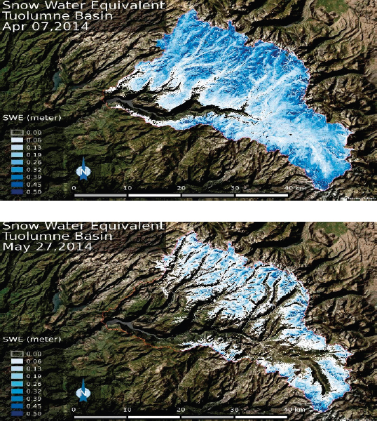
But density can also be measured either by polarimetric (Li et al., 2001) or interferometric L-band (1.4 GHz) SAR; hence, such measurements from the Program of Record (e.g., NISAR) could complement the measurement of snow depth, because density does vary in systematic ways that may affect the calculation of SWE. Generally, densities are lower at higher elevations and on slopes that receive less radiation (Wetlaufer et al., 2016).
Snow and Ice Melt
Energy used to melt seasonal snow and glaciers depends on other enabling measurements described earlier in the subsection “Energy and Water Fluxes in the Surface Layer.” Their estimation from satellite data depends on downscaling the coarse satellite estimates from instruments like CERES, along with accurate measurements of snow and ice albedo. Because many regions where snow and ice are important in the hydrologic cycle are in the mountains, many of the pixels are mixed—that is, containing some combination of snow, ice, vegetation, and soil. Spectrally unmixing these pixels and determining the albedo of the snow and ice component would be improved by measurements from a spaceborne spectrometer, which would also support information needs identified by other Decadal Survey panels—particularly ecosystems, discussed in Chapter 8.
Sublimation from Snow
Snow disappears from the land and from glaciers by two mechanisms other than snowmelt—wind transport and sublimation (the direct transition from ice to water vapor). Wind transport can be identified by measurements of snow water equivalent. Estimation of sublimation depends on many of the measurements needed to estimate evapotranspiration, with the problem being somewhat easier because the surface vapor pressure can be reliably estimated from measurement of the surface temperature.
Groundwater Storage and Recharge
Groundwater Storage and Depth to Water Table
Approximately 98 percent of all circulating freshwater (excluding glaciers and ice caps) on Earth is groundwater—that is, below the water table (Federal Council for Science and Technology, 1962). In the context of water resources, whether worldwide or in a local watershed, the groundwater stores of freshwater are vast, which is also one reason why much of the fresh groundwater is fairly old, typically a century to a millennium. That is, the larger the water volume, the longer the water residence time. In most groundwater systems, both the old and the relatively young (a few decades to a century) water is usable and replenishable, although the geology and confinement strongly affect the rate of replenishment of deeper groundwater. Aquifer replenishment occurs through recharge at the top of the groundwater system, the water table. Importantly, the recharge benefits deeper groundwater by bolstering fluid pressure, the changes in which can propagate regionally through the groundwater system much faster than the water itself.
Despite the vast volume of groundwater, only a limited quantity of it can be pumped without causing detrimental effects, which include chronic groundwater depletion, land subsidence, depletion of groundwater-dependent surface water and ecosystems, and groundwater quality degradation (e.g., seawater intrusion in coastal zones). Because of the vastness of groundwater reserves, the consequences of exploiting them, and the way that groundwater is replenished, the essential metric is the change in groundwater storage rather than the total quantity. In developed aquifer systems, changes in elevation of the water levels in wells can be measured and changes in storage calculated. Remotely sensing depth to water table with ground-penetrating radar suffers from interference from water in the soil above the groundwater.
In many parts of the world, however, measurements of depth to water table are seldom made, which is one reason why local and global awareness of major groundwater depletion in places like India, China, and North Africa did not come to light until the emergence of GRACE data (Richey et al., 2015). Moreover, even in many monitored groundwater basins and especially in the sedimentary basins that contain most of the major aquifer systems, the groundwater occurs under semiconfined conditions in which the calculation of storage change based on groundwater level data is difficult and typically infeasible without the use of well-calibrated groundwater models.
Accordingly, the capability of GRACE (Tapley et al., 2004) for detecting real-time changes in groundwater storage is in concept a highly relevant and positive development. The main limitation of GRACE is that the scale of its measurements is much larger than the scale of most groundwater systems or of typical water resources management regions. The current GRACE scale of measurement is approximately 400-500 km (Famiglietti and Rodell, 2013), while the scale of most water management basins or problems is on the order of 10-50 km (Alley and Konikow, 2015; Lakshmi, 2016). This disparity in scales of the GRACE measurements and the hydrologic system or problem means that measurements from GRACE in even large groundwater basins such as California’s Central Valley include not only the changes in groundwater storage in the major sedimentary aquifers, but also the changes in snow in the adjacent mountain range, soil moisture, and fractured-rock groundwater, which all must be measured and modeled sufficiently to separate them from the important major aquifer storage changes.
NASA announced the end of the GRACE mission in late October 2017; one of the pair of satellites has run out of fuel. The overall objectives of the GRACE-FO (to be launched in 2018) for measuring groundwater change in storage are highly relevant for both water management and understanding of global water balances. It is critically important, however, that the technology be advanced sufficiently to get the resolution down to scales relevant to water resources management (e.g., ~50 km). This scale of measurement is also most appropriate for better understanding of the almost entirely unmonitored changes in subsurface water storage in mountainous regions.
Recharge
In undeveloped groundwater systems, recharge is typically balanced by groundwater discharge (e.g., spring flow, stream baseflow, subsea discharge), driving regional and local groundwater flow system dynamics and to a large extent also keeping the groundwater systems fresh. Furthermore, in most undeveloped groundwater basins that do not discharge groundwater to oceans (e.g., Post et al., 2013), the recharge is balanced by discharge such that the net, regional recharge (i.e., recharge minus discharge) is essentially nil. Although local recharge can be substantial, net recharge does in fact depend on scale, often approaching zero at larger scales in undeveloped systems.
In developed groundwater systems, groundwater pumping can be sustainable or unsustainable, depending on whether the pumping magnitudes exceed the recharge and the reductions in natural discharge that pumping commonly induces. Accordingly, the net recharge can increase as the pumping increases and strongly influences whether the groundwater pumping will lead to unsustainable overdraft of the groundwater system.
A major unknown in both developed and undeveloped groundwater systems is the recharge. There are many ways to estimate recharge. At the landscape scale a water budget approach that accounts for precipitation, evapotranspiration, and runoff can in theory be used to calculate recharge as the residual. A major limitation of this approach is that the errors in measuring or estimating precipitation and evapotranspiration often exceed the magnitude of recharge. As the accuracy of satellite-based evapotranspiration measurements improves, direct estimation of associated recharge rates will become more feasible.
One very important case where a water balance approach has worked well for estimating recharge is in irrigated croplands, which consume more groundwater worldwide than any other use (Döll et al., 2012; Scanlon et al., 2016). Irrigation has not only caused massive, often uncontrolled increases in groundwater pumping in many parts of the world, it has also resulted in significant increases in recharge because typically only about 50 to 80 percent of the water applied to the crop is consumed (evaporated and transpired) by the crop, with most of the remainder typically recharging the groundwater. In such agricultural systems, because the evaporative water demand of the crop is easier to estimate and because the recharge tends to be greater than in nonagricultural watersheds, water budget calculations of recharge can be fairly reliable. Nevertheless, as water scarcity increases and irrigation efficiency improves, the recharge from irrigation will decrease. In turn, the need for continual, more accurate monitoring of crop evapotranspiration will only increase.
Besides irrigation water management, the other forcing that will affect recharge is climate change. Warming will tend to increase potential evapotranspiration, decreasing recharge; but on the other hand, climate-induced changes in vegetation due to reduced soil moisture and deeper groundwater levels may result in less actual evapotranspiration. Here again, our ability to monitor spatial and temporal changes in evapotranspiration, and in turn groundwater recharge and runoff, will hinge on future improvements in satellite-based methods to measure evapotranspiration.
Subsidence and Elastic Groundwater Storage Changes
Earth’s surface fluctuates both up and down due to groundwater storage changes that are referred to as either elastic or inelastic. All aquifer systems undergo elastic changes in storage wherein decreases in fluid pressure cause modest amounts of aquifer system compaction that release groundwater from storage, and increases in fluid pressure cause modest amounts of aquifer system expansion, taking groundwater into storage (Galloway et al., 2000; Amelung et al., 1999). In unconsolidated to semiconsolidated sedimentary basins that contain most of the world’s major aquifers, the aquifers are confined or semiconfined, and hence a key mechanism by which groundwater comes into or out of storage on the daily to monthly time scales is through these elastic processes, rather than solely through fluctuations of the water table
itself. In the confined and semiconfined aquifer systems, water levels in the wells are not the same as the water table, and fluctuate more than the water table by orders of magnitude, and on shorter time scales.
Whether in fresh groundwater systems, oil and gas reservoirs, or geothermal fields, the elastic changes in storage are not easily monitored. Moreover, since in most of the world including parts of the United States, groundwater levels are not sufficiently monitored, measurements of land-surface deflections caused by elastic groundwater storage changes are valuable for discerning quantities and mechanisms of groundwater storage changes (e.g., Amelung et al., 1999). Elastic changes in storage can manifest in land surface deflections on the order of 10 mm, which is within the capability of Interferometric Synthetic Aperture Radar (InSAR), which has resolution of 5-10 mm. Any future improvements in this resolution would obviously benefit real-time monitoring of groundwater storage changes, especially when complemented with information from GRACE and sparse groundwater level measurements. The finer spatial resolution of NISAR (Rosen et al., 2016) will further benefit monitoring of groundwater withdrawal consequences, as well as the subsurface geologic structures that affect it.
Subsidence, also referred to as “inelastic compaction,” occurs when declines in fluid pressure are sufficient to increase effective stress (sediment grain-to-grain stresses) to an extent not previously experienced in the geologic burial history of the sedimentary package of coarse and fine sediments (Galloway et al., 2000). This important form of groundwater overdraft is increasingly symptomatic of increasing overexploitation of groundwater resources. Prior to availability of InSAR, real-time knowledge of subsidence and its associated, permanent losses in groundwater storage capacity and damage to surface structures did not come to light until the damage was already done. InSAR revolutionized our ability to monitor subsidence in real time and led to unanticipated discoveries about use of land-surface data for determining previously unrecognized subsurface complexities. Again, NISAR and future missions will significantly enhance this capability.
High-resolution GPS monitoring of the land surface has also recently been used to detect cm-scale deflections in Earth’s crust in response to crustal loading and unloading caused by total change in subsurface water content (Borsa et al., 2014). Future improvements in tracking not only subsidence but also groundwater storage will lie in the joint use of GRACE, InSAR, NISAR, and GPS. Collectively, this approach will become increasingly essential for local and regional groundwater management.
Water Quality
One of the essential but overlooked elements of regional water availability and sustainable water resources management is water quality. Water quality issues are local and need to be observed at a finer temporal and spatial resolution in order to be used and incorporated into local decision making. Some progress has been made utilizing satellite-based observations for monitoring and assessing eutrophication impacts in coastal waters (Schaeffer et al., 2012, 2013). However, the current technologies embedded in our Earth observing satellite systems are not adequate to gather the kind of signals that could be used to infer various biological, chemical, or physical variables at a finer scale to map regional or local water quality. The pixel resolution of platforms such as MODIS and Landsat or the forthcoming Sentinel 3 mission is too coarse for this purpose (Lee et al., 2014).
In order to evaluate and manage water quality for inland waters, we need to measure turbidity, salinity, colored dissolved organic matter (CDOM), temperature, sediment load, and chlorophyll-a. Spatial resolution of 30-60 m is required in order to have observations that are interpretable and detectable to evaluate the state of inland water bodies such as rivers and lakes at various geographical scales (Hestir et al., 2015; Turpie et al., 2015). The desired temporal resolution is daily to weekly observations.
Advancement in spectrometer imaging technologies, at spatial scales of rivers, inland water bodies, and coastal regions, can ultimately address some of these problems. More focus is also needed on developing
algorithms to infer water quality variables based on receiving signals while addressing land adjacency and atmospheric effects (Lee et al., 2014). In addition, considering the advancement of drones and other imaging technologies, there are possibilities for regions with extensive water quality challenges to rely on these technologies to collect water quality data at a finer temporal and spatial scale.
In January 2017, NASA Earth Sciences Division (ESD) issued solicitation A.30 Remote Sensing of Water Quality, to identify investigations that could improve the measurement of water quality from spaceborne and airborne sensors. Selections for the funded investigations were announced in July 2017. Findings from them could affect future recommendations and prospects for remotely sensing water quality from space.
Land Use and Land Cover
Vegetation Species
There has been a long and successful history of obtaining vegetation classifications at the community level with existing sensors such as Landsat, SPOT, and MODIS (Xie et al., 2008). Classification and mapping at the species level requires finer spatial resolution, generally less than 5 m (IKONOS, Quickbird). Classification at the community or species level does not generally provide the condition of the vegetation—for example, whether a grassland’s grass is 50 cm or 2 cm tall, owing to grazing or different stages in growth phenology. Finer spatial resolution multispectral sensors will be required for more reliable identification of plant species.
The relative vigor or level of plant stress is another important attribute to constrain evapotranspiration estimates that is not measured by community- or species-level classifications. Thermal remotely sensed measurements have been used as a measure of plant moisture stress to improve evapotranspiration retrievals (Anderson et al., 2004, 2007) also the subsection “Diurnal Cycle of Surface Temperature,” earlier). Another relatively recent technique to measure plant vigor is through solar-induced chlorophyll fluorescence (SIF; Joiner et al., 2011). SIF is an indicator of photosynthetic activity and efficiency at the molecular scale (Meroni et al., 2009). When plants are water or temperature limited, photosynthesis is reduced but light absorption continues. To compensate, plants decrease the release of fluorescent photons at wavelengths of 690 to 800 nm. Imaging spectrometers with ultra-fine spectral resolution (0.02-0.05 nm full-width half-maximum) in the range centered around 760 nm now enable accurate and global fluorescence retrieval (Frankenberg et al., 2013). The Greenhouse Gases Observing Satellite (GOSAT) and the Orbiting Carbon Observatory-2 (OCO-2) have spectrometers that enable retrieval of chlorophyll fluorescence (Frankenberg et al., 2012). The ESA Fluorescence Explorer (FLEX) is designed specifically to monitor global terrestrial vegetation for steady-state chlorophyll fluorescence and is scheduled to be launched in 2022.
Vegetation Structure
As noted earlier, spectral remote-sensing methods have had less success in complex multispecies stands where overstory shading, interwoven branches, and understory plants are present. Light detection and ranging (lidar) can address many of the shortcomings of spectrum-based remote sensing. With high pulse rates exceeding 500,000 pulses per second, airborne systems can achieve ~10 to 30 multireturn points per square meter. Even in dense foliage, lidar point returns (x, y, z, and returned intensity) typically sample not only the top of the canopy and ground but also numerous points within the canopy. Resulting point clouds can be analyzed for a variety of vegetation structural attributes. If the plant species is also known, greater inferences can be made regarding plant structure using species-specific allometric relationships such as LAI, biomass, and aboveground carbon. Multisensor airborne lidar systems with co-registered multispectral sensors are available to simultaneously tackle the vegetation species identification and vegetation structure estimation.
Single-photon counting lidar systems are advancing rapidly, and a 10-kHz system is being deployed on the upcoming 2018 IceSAT-2 mission in the Advanced Topographic Laser Altimeter System (ATLAS) instrument. This system will provide point returns along six tracks at a spacing of roughly 70 cm. Ideally, a future system could provide ground point densities of approximately 8 points per square meters on biweekly or monthly time scales to provide growth phenology. Growth phenology of major commodity crops, coupled with plant growth models, would provide a powerful tool for improved crop market projections and early warning of famine. Synchronized lidar and traditional multispectral and narrow-band spectrometer measurements coupled with multidata fusion techniques would further address multiple research objectives recommended by several other Decadal Survey panels.
RESULTING SOCIETAL BENEFIT
The crucial question for our interactions with water is: How can we protect ecosystems and better manage and predict water availability and quality for future generations, given changes to the water cycle caused by human activities and climate trends? The problem of sustainable water resources management is itself a grand research challenge not only because prediction of future forcings is challenging but also because real-time measurements of the state of the hydrologic systems, including the essential stores and fluxes of surface water and groundwater, are commonly lacking (NRC, 2012, 1991). The recommended enhancements to remote sensing of the water cycle focus on critical research questions and provide insights that enable us to address societal needs for understanding of water systems. Water will become even more critical and difficult to manage in a highly variable future that involves new and growing stressors on the global water resource, all of which contribute to changes in quality, quantity, and availability of water (Zimmerman et al., 2008). These stressors—changing climate, evolving land use and urbanization, shifting water demands for food, energy and fiber, growing and migrating populations, and individual and societal decisions—complicate efforts to ensure clean water to support humans and ecosystems. Balancing the needs of water for people and water for critical and sensitive ecosystems presents a significant challenge for natural, social, and engineering science. There is widespread agreement with regard to the need to develop methods and application-oriented frameworks for using satellite data in water and ecosystems resources management, to monitor and protect public health and agriculture, and to manage disaster preparedness and response (Hossain et al., 2016).
Use of Remotely Sensed Data to Manage Water
NASA’s Applied Earth Sciences Program has developed over the last decade a portfolio of demonstration activities focused on transferring research to operations, toward bringing NASA’s observations and models to national and international partners through regional centers (e.g., the SERVIR network), training programs, and capacity building. A track record of successful collaborations with the Federal Emergency Management Agency (FEMA) and state agencies already exists, including reconnaissance of the 2016 Mississippi and Louisiana flooding to support FEMA disaster response. Increasing the use of satellite-based observations by the public in the future requires a comprehensive understanding of how observations and models are integrated in sector-specific decision making toward providing products with information content tailored to meet stakeholder needs. For example, reservoir operations for flood control, water supply, and power generation benefit from river forecasts (Boucher et al., 2012), and more accurate forecasts permit more effective reservoir operations, either through improved seasonal forecasts via improved initial conditions or via more accurate interannual meteorological forecasts (Anghileri et al., 2016). Enhancements to both the initial conditions and the interannual forecasts will be enabled by the
goals, objectives, and measurements proposed here. Estimates of snow water equivalent drive many of the water supply forecasts, especially in the western United States. The measurements and the modeling that will result are specifically designed to improve basin snow water equivalent estimates that can be used to update forecast model states. Objective H-1a includes measuring evaporation more accurately, thereby leading to improved formulations of the evaporative fluxes in both meteorological and hydrologic models, which can lead to improvements in the interannual forecasts. Availability of reliable information about water at scales from small basins to Earth itself can improve decisions. Recognizing that decisions about managing water and adapting to its scarcities and abundance will be made regardless of the availability of information, we can examine instances where better information has led to decisions that benefit society, by increasing revenues, decreasing costs, or providing humanitarian benefits that are harder to measure but at least as valuable. In addition, understanding how information is used by various decision makers or planners is key toward developing more effective use of models and tools in water management (Meyer et al., 2013; Matte et al., 2017; Thiboult et al., 2017).
Groundwater at the Scale of Management Decisions
A major challenge in hydrology and water resources management is the lack of integration of groundwater and surface water. This challenge is directly linked to the considerable difficulty of measuring groundwater recharge, which is largely the residual of precipitation and evapotranspiration. Unfortunately, the errors inherent to measurements of precipitation and evapotranspiration often exceed the magnitudes of recharge, rendering this key coupling between surface water and groundwater poorly defined in the past, present, and future. The ongoing improvements in remote sensing of precipitation and evapotranspiration will significantly improve our ability to better couple the surface and subsurface parts of the hydrologic cycle. With current knowledge, directly remotely sensing groundwater storage is feasible only at very coarse scales using GRACE (Richey et al., 2015) or possibly by examining hysteresis in elastic subsidence and rebound, for which there is some intriguing evidence (Chaussard et al., 2014). Inelastic subsidence, whereby groundwater withdrawals have permanently lowered the land surface, has been measured with InSAR (Amelung et al., 1999), but at that point the nonsustainable withdrawal of groundwater has already occurred. Sustainably managing all the major stores of circulating freshwater, most of which are in the subsurface, would benefit from a technology to measure changes in groundwater storage at a scale at which basins are managed, ~50 km. As of the date of publication of this Decadal Survey, such a technology with sufficient evidence of its usefulness does not exist. A GRACE-like instrument would be useful at 50 km resolution, but the GRACE-FO does not achieve that. InSAR has applications in other areas of Earth science, and if such a technology is selected for launch in the 2024-2034 time frame, then exploring its use in estimating groundwater balance through measurement of elastic subsidence is a fruitful research area for NASA and its partners.
Remote Sensing of Snow Water Equivalent
Figure 6.12 shows an example of how remotely sensed information increased confidence in water management. The Tuolumne River in California’s Sierra Nevada flows into Hetch Hetchy Reservoir, which supplies water for San Francisco, protects against downstream floods, and generates hydropower. Managing the quantity of water stored in the reservoir thus addresses competing interests: keeping the reservoir as full as possible increases the supply of water, maintaining a buffer below its capacity protects against floods, and releasing water to generate hydropower produces income. Operating the reservoir uses estimates about the snow water equivalent remaining in the basin above the reservoir. Historically, this information comes from
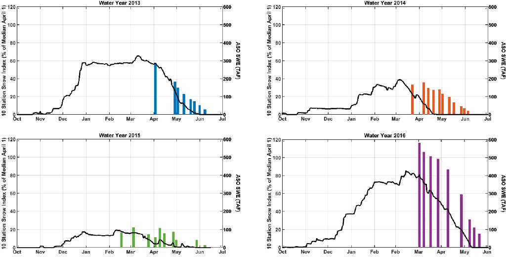
a network of snow sensors, but since 2013 NASA’s Airborne Snow Observatory (Painter et al., 2016) has measured spatially distributed snow depth weekly in the springtime from near-peak accumulation through the end of the snowmelt season with a scanning lidar. Snow water equivalent is estimated by multiplying these values with snow density, which is determined from measurements at snow sensors in the basin and interpolated in combination with a snowmelt model. ASO’s imaging spectrometer measure snows albedo.
In the first year of operation, 2013, the surface network showed the same picture about the remaining snow as the ASO. From 2013 to 2016 Hetch Hetchy Water and Power (HHWP, part of San Francisco’s Public Utilities Commission) found that accumulated inflow to the reservoir from dates of ASO acquisition through the end of July in each year strongly correlated (R2 > 0.99) with a linear combination of ASO’s measurement of the total basin snowpack and local rainfall during the melt season. These years spanned a historically severe drought from 2013 to 2015 and a near average year of 2016.
In 2013 reservoir managers were happy to see that the remotely sensed observations confirmed what they already knew. Then in 2014, and again in 2016, ASO showed more snow remaining in the basin than the surface network showed (see Figure 6.12), because in those years a different pattern of snow accumulation produced more snow at the higher elevations that are not sampled well by the surface network. HHWP has long used a composite of snow sensors in and surrounding the Tuolumne River Basin to estimate the accumulation and melt of snow in the basin. ASO’s measurement of the distribution of snow water equivalent (see Figure 6.11) showed that in 2014, when snow at all the sensors had melted, ASO showed that 85 percent of peak water equivalent remained in the basin.
The robustness of the relationship between runoff and ASO gave HHWP far greater confidence in water management decisions in these critical drought years.
Management of Agricultural Lands
Other examples exist of operational implementation of satellite-based Earth observations and modeling for improved water resources management. The NASA Applied Sciences Water Resources Program (https://appliedsciences.nasa.gov/programs/water-resources-program) supports several efforts including mapping of fallowed area for regional agricultural drought impact assessment, water supply forecasting, regional drought monitoring, optimization of reservoir operations for hydropower, and improved global crop production decision support.
One example includes a joint project with the California Department of Water Resources (CDWR); U.S. Department of Agriculture (USDA); U.S. Geological Survey (USGS); NASA Ames Research Center; and California State University, Monterey Bay (CSUMB). Landsat data are being used to track the extent of fallowed land in the Central Valley of California using satellite imagery including Landsat 5, 7, and 8 (Figure 6.13). Project partners are now working to establish an operational fallowed land monitoring service as part of a California drought early warning information system, a pilot of the National Integrated Drought Information System (NIDIS) led by NOAA. This effort is helping estimate the economic impacts of drought events—for example, the system helped confirm model-based estimates of 1.91 million acres of fallowed land during the 2015 drought in California Central Valley—an increase of 540,000 acres relative to recent years with similar average precipitation across the state.
Few rigorous studies have thoroughly demonstrated the socioeconomic benefits of satellite data applications for improve water resources management. One example included an econometric analysis to characterize the contribution of assimilating GRACE data into the U.S. Drought Monitor (Svoboda et al., 2002) to capture the effects of drought on the agricultural sector. The study employed a multimethod approach to constrain prior and posterior decision-maker beliefs based on GRACE-enhanced observations to estimate economic value of information (Bernknopf and Shapiro, 2015). In this way the method illustrates the risk and potential impact of management decisions from drought events captured (and missed) by the USDM from 2002 to 2013. Results indicate that the sum of errors from the addition of GRACE data assimilation is reduced by roughly $1.1 billion per year (Long et al., 2013; Richey et al., 2015). In addition, the study illustrates how careful integration of satellite-based observations in an operational system such as the USDM can lead to meaningful changes in a policy-making setting.
Another study used a conceptual framework and multiple environmental models to assess the socioeconomic impact of Landsat-based agricultural mapping and groundwater quality (Forney et al., 2012). Effects of dynamic nitrogen loading and transport were considered based on specified distances from specific wells and at landscape scales. Mapped land for corn and soybean production in northeastern Iowa was used to assess the risk of groundwater contamination if corn and soybean production were moved to lands identified to be less prone to leach nitrate (Figure 6.14). The marginal benefit of the Moderate-Resolution Land Imagery (MRLI) value of information (VOI) in 2010 dollars is $858 million ± $197 million annualized.
Floods and Droughts
Globally, floods have accounted for 47 percent of all weather-related disasters, affecting 2.3 billion people. The number of floods per year rose to an average of 171 in the period 2005-2014, up from an annual average of 127 in the previous decade (UNISDR, 2015). Flood events amount to several-billion-dollar costs, up to $4 billion in the United States alone.
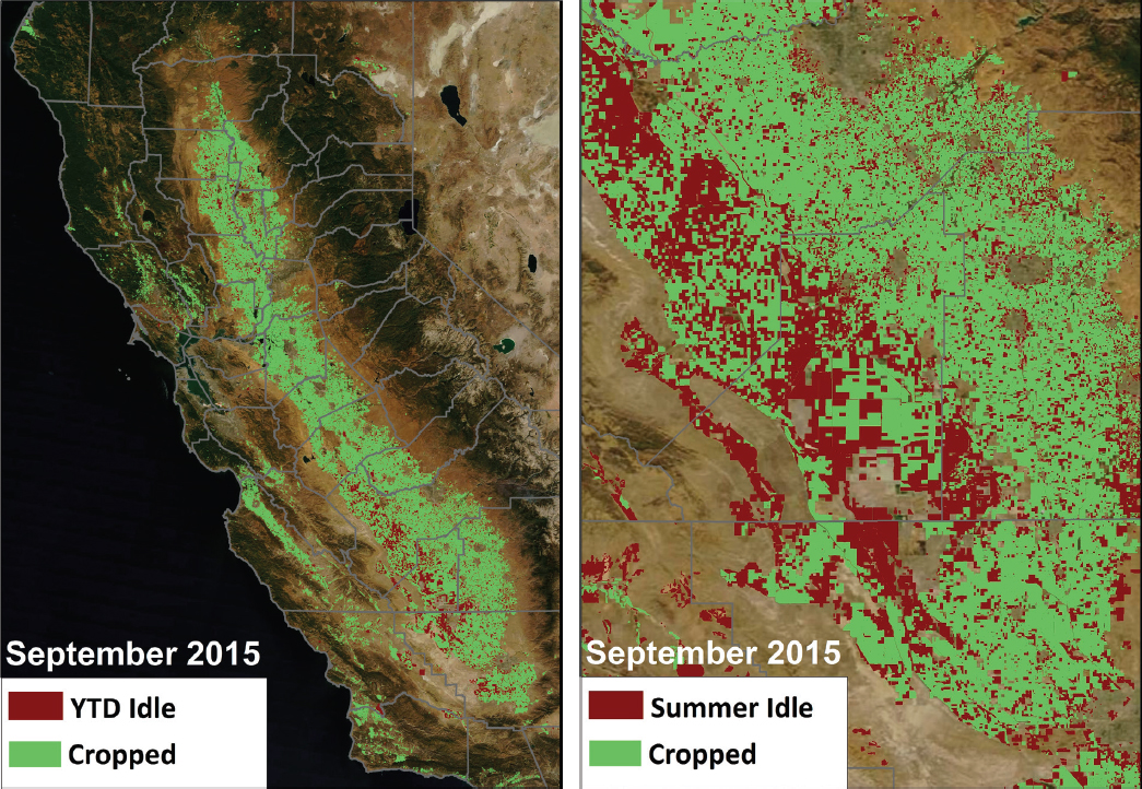
Drought prediction and mitigation offers another example of direct societal benefit from the remote sensing measurements listed in this report. Over the last two decades, over 1 billion people have been affected by drought (1995-2015) due to food insecurity, which compounded with water shortages and water quality results in long-term impacts on public health and ecosystems (UNISDR, 2015). In 2016, droughts were estimated to have cost the United States $3.5 billion; in 2015, that same drought cost the United States $4.5 billion, and wildfires, whose likelihood are increased in drought conditions, cost an additional $1 billion in the western United States and Alaska. The 2012 drought cost is estimated at $30 billion and 123 deaths, with an additional $10 billion and 53 deaths in 2013 (NOAA NCDC, 2017). Predicting drought onset and end depends on currently uncertain long-range precipitation predictions and good soil moisture measurements (Wood et al., 2015). In snow-dominated watersheds, seasonal drought is predictable if the snow accumulation can be assessed near the beginning of the melt season. Snow-covered area can be derived from remotely sensed data, but in the mountainous areas where the winter snowpack is deep, passive microwave sensors are ineffective; hence the high priority for Objective H-1c.
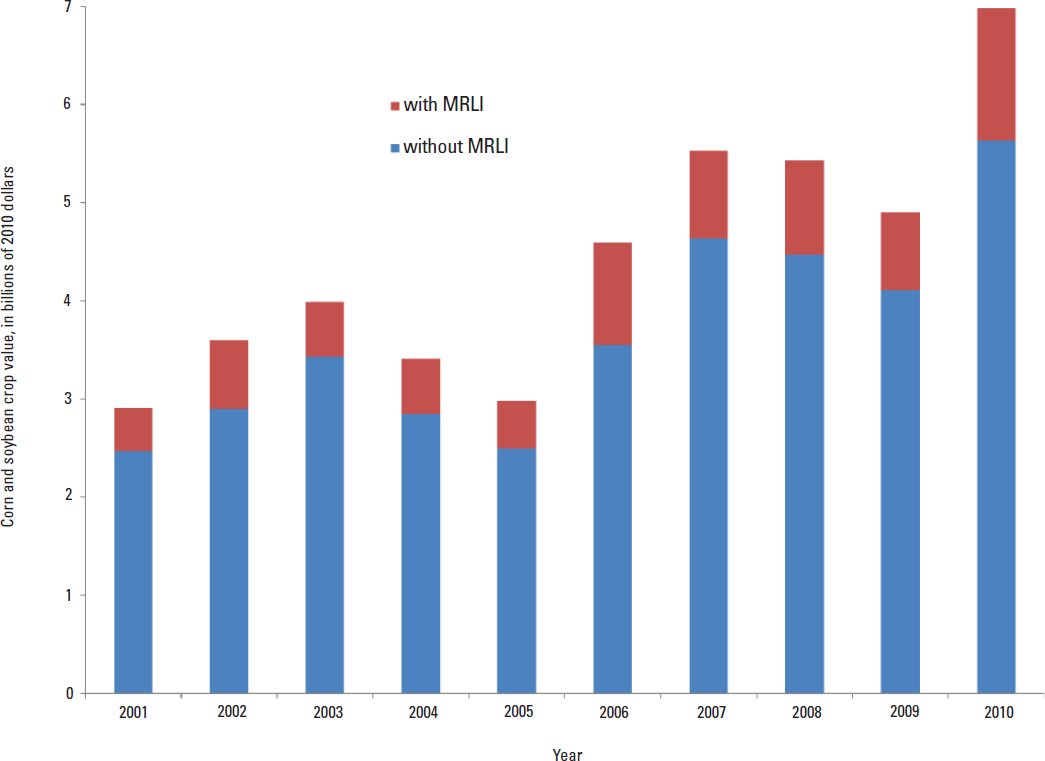
Objectives H-1a, H-1b, and H-1c, along with H-2a, combine to quantify the major fluxes of the water cycle, and will be essential contributors to the improvement of the precipitation forecasts. In this case the societal benefit will result from the combination of existing measurement programs (SMAP) with new measurements. Even slight improvements in our ability to manage our water resources to mitigate drought impacts can potentially save many millions of dollars. Conceptually, we understand the water cycle, but our quantitative understanding of its components is limited to some fluxes—streamflow and precipitation, for example—and surface water stores (NRC, 1991, 2002, 2008). Climate change, however, causes changes in vegetation, human extraction of water, the rain-snow transition, and the timing and severity of storms. These changes in turn alter soil properties, channel networks, and other landscape features. Current surface monitoring networks were never designed to examine these factors together, yet remote sensing technologies enable this type of integrated data collection.
Integration with Climate Models
We could list many examples here where recommended advances in remote sensing address gaps in measurements, which in turn inhibit understanding. Choosing one, models of future climate agree better with each other about future temperatures than about future precipitation and evapotranspiration (Coquard et al., 2004). An impediment to progress is that the measurements of precipitation that include both rain and snow are not sufficient to validate numerical weather predictions—for example, sites where precipitation or snow accumulation is measured are generally on flat ground, even on mountain summits, and in most mountain ranges do not extend to the highest elevations where precipitation occurs. Remote sensing can help with this validation through strategies to integrate measured values over the scales of models’ grid cells.
Design and operation of water infrastructure have traditionally relied on empirical relationships and engineering experience. Unfortunately, because of our need for ongoing operation of our distributed water infrastructure under dynamic and locally distinct conditions, there are significant gaps in our understanding that are critical for improved operation, maintenance, and future design. Because we cannot turn off our systems or test them to failure, we make small changes to adapt to new conditions, but we cannot evaluate changes at the scale of operational systems or with consideration of the complete engineered water cycle. The small changes we can make enable incremental improvements, but they do not necessarily advance our understanding to a state where we could operate or optimize under different conditions, including energy management.
REFERENCES
Abdalati, W., H.J. Zwally, R. Bindschadler, B. Csatho, S.L. Farrell, H.A. Fricker, D. Harding, et al. 2010. The ICESat-2 laser altimetry mission. Proceedings of the IEEE 98(5):735-751.
Acclimatise. 2014. “Climate change resilience in Europe: A snapshot of the private sector.” http://www.acclimatise.uk.com/login/uploaded/resources/CDP_Document.pdf.
Adams, H.D., C.H. Luce, D.D. Breshears, C.D. Allen, M. Weiler, V.C. Hale, A.M.S. Smith, and T.E. Huxman. 2012. Ecohydrological consequences of drought- and infestation-triggered tree die-off: Insights and hypotheses. Ecohydrology 5(2):145-159.
Adams-Selin, R.D., S.C. van den Heever, and R.H. Johnson. 2013. Impact of graupel parameterization schemes on idealized bow echo simulations. Monthly Weather Review 141(4):1241-1262.
Adikari, Y., and J. Yoshitani. 2009. Global Trends in Water-Related Disasters: An Insight for Policymakers. Paris: UNESCO.
Adler, R.F., G.J. Huffman, A. Chang, R. Ferraro, P.P. Xie, J. Janowiak, B. Rudolf, et al. 2003. The Version-2 Global Precipitation Climatology Project (GPCP) monthly precipitation analysis (1979-present). Journal of Hydrometeorology 4(6):1147-1167.
AghaKouchak, A., L. Cheng, O. Mazdiyasni, and A. Farahmand. 2014. Global warming and changes in risk of concurrent climate extremes: Insights from the 2014 California drought. Geophysical Research Letters 41(24):8847-8852.
Ahearn, D.S., R.W. Sheibley, R.A. Dahlgren, M. Anderson, J. Johnson, and K.W. Tate. 2005. Land use and land cover influence on water quality in the last free-flowing river draining the Western Sierra Nevada, California. Journal of Hydrology 313(3-4):234-247.
Ajami, N.K., B.H. Thompson Jr., and D.G. Victor. 2014. The Path to Water Innovation. Washington, DC: Brookings Institution.
Akbar, R., N. Das, D. Entekhabi, and M. Moghaddam. 2016. Active and passive microwave remote sensing synergy for soil moisture estimation. Pp. 187-208 in Satellite Soil Moisture Retrieval: Techniques and Applications (P.K. Srivastava, G.P. Petropoulos, and Y.H. Kerr, eds.). Amsterdam: Elsevier.
Akhtar, M.K., G.A. Corzo, S.J. van Andel, and A. Jonoski. 2009. River flow forecasting with artificial neural networks using satellite observed precipitation pre-processed with flow length and travel time information: Case study of the Ganges river basin. Hydrology and Earth System Sciences 13(9):1607-1618.
Alexander, L.V., X. Zhang, T.C. Peterson, J. Caesar, B. Gleason, A.M.G. Klein Tank, M. Haylock, et al. 2006. Global observed changes in daily climate extremes of temperature and precipitation. Journal of Geophysical Research: Atmospheres 111(D5):D05109.
Allan, D., D. Erickson, and J. Fay. 1997. The influence of catchment land use on stream integrity across multiple spatial scales. Freshwater Biology 37(1):149-161.
Alley, W.M., and L.F. Konikow. 2015. Bringing GRACE down to earth. Groundwater 53(6):826-829.
Amelung, F., D.L. Galloway, J.W. Bell, H.A. Zebker, and R.J. Laczniak. 1999. Sensing the ups and downs of Las Vegas: InSAR reveals structural control of land subsidence and aquifer-system deformation. Geology 27(6):483-486.
AmeriFlux. 2017. “AmeriFlux Network.” http://ameriflux.lbl.gov/. Accessed April 5, 2018.
Ampe, E.M., D. Raymaekers, E.L. Hestir, M. Jansen, E. Knaeps, and O. Batelaan. 2015. A wavelet-enhanced inversion method for water quality retrieval from high spectral resolution data for complex waters. IEEE Transactions on Geoscience and Remote Sensing 53(2):869-882.
Anderegg, W.R.L., J.M. Kane, and L.D.L. Anderegg. 2013. Consequences of widespread tree mortality triggered by drought and temperature stress. Nature Climate Change 3(1):30-36.
Anderson, M.C., C. Hain, B. Wardlow, A. Pimstein, J.R. Mecikalski, and W.P. Kustas. 2011. Evaluation of drought indices based on thermal remote sensing of evapotranspiration over the Continental United States. Journal of Climate 24(8):2025-2044.
Anderson, M.C., J.M. Norman, J.R. Mecikalski, J.A. Otkin, and W.P. Kustas. 2007. A climatological study of evapotranspiration and moisture stress across the continental United States based on thermal remote sensing: 1. Model formulation. Journal of Geophysical Research: Atmospheres 112(D10).
Anderson, M.C., J.M. Norman, J.R. Mecikalski, R.D. Torn, W.P. Kustas, and J.B. Basara. 2004. A multiscale remote sensing model for disaggregating regional fluxes to micrometeorological scales. Journal of Hydrometeorology 5(2):343-363.
Anghileri, D., N. Voisin, A. Castelletti, F. Pianosi, B. Nijssen, and D.P. Lettenmaier. 2016. Value of long-term streamflow forecasts to reservoir operations for water supply in snow-dominated river catchments. Water Resources Research 52(6):4209-4225.
Aragão, L.E.O.C. 2012. The rainforest’s water pump. Nature 489(7415):217-218.
Armstrong, P. 2014. The Log of a Snow Survey: Skiing and Working in a Mountain Winter World. Bloomington, Ind.: Abbott Press.
Arnold, J.G., and N. Fohrer. 2005. SWAT2000: Current capabilities and research opportunities in applied watershed modelling. Hydrological Processes 19(3):563-572.
Ashley, S.T., and W.S. Ashley. 2008. Flood fatalities in the United States. Journal of Applied Meteorology and Climatology 47(3):805-818.
Ashouri, H., K.L. Hsu, S. Sorooshian, D.K. Braithwaite, K.R. Knapp, L.D. Cecil, B.R. Nelson, and O.P. Prat. 2015. PERSIANN-CDR: Daily precipitation climate data record from multisatellite observations for hydrological and climate studies. Bulletin of the American Meteorological Society 96(1):69-83.
Asner, G.P., J. Mascaro, H.C. Muller-Landau, G. Vieilledent, R. Vaudry, M. Rasamoelina, J.S. Hall, and M. Van Breugel. 2012. A universal airborne lidar approach for tropical forest carbon mapping. Oecologia 168(4):1147-1160.
August, T., D. Klaes, P. Schlüssel, T. Hultberg, M. Crapeau, A. Arriaga, A. O’Carroll, D. Coppens, R. Munro, and X. Calbet. 2012. IASI on Metop-A: Operational level 2 retrievals after five years in orbit. Journal of Quantitative Spectroscopy and Radiative Transfer 113(11):1340-1371.
Bair, E.H., R.E. Davis, and J. Dozier. 2017. Hourly mass and snow energy balance measurements from Mammoth Mountain, CA USA, 2011-2017. Earth System Science Data Discussion 2017:1-15.
Bair, E.H., K. Rittger, R.E. Davis, T.H. Painter, and J. Dozier. 2016. Validating reconstruction of snow water equivalent in California’s Sierra Nevada using measurements from the NASA Airborne Snow Observatory. Water Resources Research 52:8437-8460.
Bajracharya, B., A.B. Shrestha, and L. Rajbhandari. 2007. Glacial lake outburst floods in the Sagarmatha region. Mountain Research and Development 27(4):336-344.
Baldocchi, D., E. Falge, L. Gu, R. Olson, D. Hollinger, S. Running, P. Anthoni, et al. 2001. FLUXNET: A new tool to study the temporal and spatial variability of ecosystem-scale carbon dioxide, water vapor, and energy flux densities. Bulletin of the American Meteorological Society 82(11):2415-2434.
Bales, R.C., N.P. Molotch, T.H. Painter, M.D. Dettinger, R. Rice, and J. Dozier. 2006. Mountain hydrology of the Western United States. Water Resources Research 42:W08432.
Barnett, T.P., J.C. Adam, and D.P. Lettenmaier. 2005. Potential impacts of a warming climate on water availability in snow-dominated regions. Nature 438:303-309.
Barros, A.P. 2013. Orographic precipitation, freshwater resources, and climate vulnerabilities in mountainous regions. Pp. 57-58 in Climate Vulnerability: Understanding and Addressing Threats to Essential Resources (R. Pielke, ed.). Oxford: Academic Press.
Barros, A.P., Y. Duan, J. Brun, and M.A. Medina. 2014. Flood nonstationarity in the Southeast and Mid-Atlantic regions of the United States. Journal of Hydrologic Engineering 19(10):05014014.
Barros, A.P., J.L. Hodes, and M. Arulraj. 2017. Decadal climate variability and the spatial organization of deep hydrological drought. Environmental Research Letters 12(10):104005.
Barros, A.P., G. Kim, E. Williams, and S.W. Nesbitt. 2004. Probing orographic controls in the Himalayas during the monsoon using satellite imagery. Natural Hazards and Earth System Sciences 4(1):29-51.
Barros, A.P., and T.J. Lang. 2003. Monitoring the monsoon in the Himalayas: Observations in Central Nepal, June 2001. Monthly Weather Review 131(7):1408-1427.
Bauer, P., A. Thorpe, and G. Brunet. 2015. The quiet revolution of numerical weather prediction. Nature 525(7567):47-55.
Belmont, P., K.B. Gran, S.P. Schottler, P.R. Wilcock, S.S. Day, C. Jennings, J.W. Lauer, E. Viparelli, J.K. Willenbring, D.R. Engstrom, and G. Parker. 2011. Large shift in source of fine sediment in the Upper Mississippi River. Environmental Science & Technology 45(20):8804-8810.
Benjamin, S.G., S.S. Weygandt, J.M. Brown, M. Hu, C.R. Alexander, T.G. Smirnova, J.B. Olson, et al. 2015. A North American hourly assimilation and model forecast cycle: The rapid refresh. Monthly Weather Review 144(4):1669-1694.
Benson, E. 2012. One infrastructure, many global visions: The commercialization and diversification of Argos, a satellite-based environmental surveillance system. Social Studies of Science 42(6):843-868.
Berg, P., C. Moseley, and J.O. Haerter. 2013. Strong increase in convective precipitation in response to higher temperatures. Nature Geoscience 6(3):181-185.
Berg, W., S. Bilanow, R. Chen, S. Datta, D. Draper, H. Ebrahimi, S. Farrar, et al. 2016. Intercalibration of the GPM microwave radiometer constellation. Journal of Atmospheric and Oceanic Technology 33(12):2639-2654.
Berggren, K., M. Olofsson, M. Viklander, G. Svensson, and A.M. Gustafsson. 2012. Hydraulic Impacts on urban drainage systems due to changes in rainfall caused by climatic change. Journal of Hydrologic Engineering 17(1):92-98.
Berne, A., G. Delrieu, J.D. Creutin, and C. Obled. 2004. Temporal and spatial resolution of rainfall measurements required for urban hydrology. Journal of Hydrology 299(3):166-179.
Bernknopf, R., and C. Shapiro. 2015. Economic assessment of the use value of geospatial information. ISPRS International Journal of Geo-Information 4(3):1142-1165.
Betts, A.K. 2004. Understanding hydrometeorology using global models. Bulletin of the American Meteorological Society 85(11):1673-1688.
Betts, A.K., J.H. Ball, A.C.M. Beljaars, M.J. Miller, and P.A. Viterbo. 1996. The land surface-atmosphere interaction: A review based on observational and global modeling perspectives. Journal of Geophysical Research: Atmospheres 101(D3):7209-7225.
Bhutiyani, M.R., V.S. Kale, and N.J. Pawar. 2010. Climate change and the precipitation variations in the northwestern Himalaya: 1866-2006. International Journal of Climatology 30(4):535-548.
Biancamaria, S., D.P. Lettenmaier, and T.M. Pavelsky. 2016. The SWOT mission and its capabilities for land hydrology. Surveys in Geophysics 37(2):307-337.
Biederman, J.A., A.J. Somor, A.A. Harpold, E.D. Gutmann, D.D. Breshears, P.A. Troch, D.J. Gochis, R.L. Scott, A.J.H. Meddens, and P.D. Brooks. 2015. Recent tree die-off has little effect on streamflow in contrast to expected increases from historical studies. Water Resources Research 51(12):9775-9789.
Bladon, K.D., U. Silins, M.J. Wagner, M. Stone, M.B. Emelko, C.A. Mendoza, K.J. Devito, and S. Boon. 2008. Wildfire impacts on nitrogen concentration and production from headwater streams in southern Alberta’s Rocky Mountains. Canadian Journal of Forest Research 38(9):2359-2371.
Blann, K.L., J.L. Anderson, G.R. Sands, and B. Vondracek. 2009. Effects of agricultural drainage on aquatic ecosystems: A review. Critical Reviews in Environmental Science and Technology 39(11):909-1001.
Bolten, J.D., W.T. Crow, X. Zhan, T.J. Jackson, and C.A. Reynolds. 2010. Evaluating the utility of remotely sensed soil moisture retrievals for operational agricultural drought monitoring. IEEE Journal of Selected Topics in Applied Earth Observations and Remote Sensing 3(1):57-66.
Bondeau, A., P.C. Smith, S. Zaehle, S. Schaphoff, W. Lucht, W. Cramer, D. Gerten, H. Lotze-Campen, C. Müller, M. Reichstein, and B. Smith. 2007. Modelling the role of agriculture for the 20th century global terrestrial carbon balance. Global Change Biology 13(3):679-706.
Borsa, A.A., D.C. Agnew, and D.R. Cayan. 2014. Ongoing drought-induced uplift in the western United States. Science 345(6204):1587-1590.
Boucher, M.A., D. Tremblay, L. Delorme, L. Perreault, and F. Anctil. 2012. Hydro-economic assessment of hydrological forecasting systems. Journal of Hydrology 416:133-144.
Brocca, L., S. Hasenauer, T. Lacava, F. Melone, T. Moramarco, W. Wagner, W. Dorigo, et al. 2011. Soil moisture estimation through ASCAT and AMSR-E sensors: An intercomparison and validation study across Europe. Remote Sensing of Environment 115(12):3390-3408.
Brown, S.A., J.D. Schall, J.L. Morris, C.L. Doherty, S.M. Stein, and J.C. Warner. 2009. Urban Drainage Design Manual. Washington, DC: Federal Highway Administration.
Brun, J., and A.P. Barros. 2014. Mapping the role of tropical cyclones on the hydroclimate of the southeast United States: 2002-2011. International Journal of Climatology 34(2):494-517.
Bryan, G.H., and H. Morrison. 2012. Sensitivity of a simulated squall line to horizontal resolution and parameterization of microphysics. Monthly Weather Review 140(1):202-225.
Burgin, M.S., A. Colliander, E.G. Njoku, S.K. Chan, F. Cabot, Y.H. Kerr, R. Bindlish, T.J. Jackson, D. Entekhabi, and S.H. Yueh. 2017. A comparative study of the SMAP passive soil moisture product with existing satellite-based soil moisture products. IEEE Transactions on Geoscience and Remote Sensing 55(5):2959-2971.
Burke, M.P., T.S. Hogue, A.M. Kinoshita, J. Barco, C. Wessel, and E.D. Stein. 2013. Pre-and post-fire pollutant loads in an urban fringe watershed in Southern California. Environmental Monitoring and Assessment 185(12):10131-10145.
Campolo, M., A. Soldati, and P. Andreussi. 2003. Artificial neural network approach to flood forecasting in the River Arno. Hydrological Sciences Journal 48(3):381-398.
Canadell, J.G., H.A. Mooney, D.D. Baldocchi, J.A. Berry, J.R. Ehleringer, C.B. Field, S.T. Gower, et al. 2000. Carbon metabolism of the terrestrial biosphere: A multitechnique approach for improved understanding. Ecosystems 3(2):115-130.
Cannon Leahy, T. 2016. Desperate times call for sensible measures: The making of the California Sustainable Groundwater Management Act. Golden Gate University Environmental Law Journal 9(1):5-40.
Chaney, N.W., P. Metcalfe, and E.F. Wood. 2016. HydroBlocks: A field-scale resolving land surface model for application over continental extents. Hydrological Processes 30(20):3543-3559.
Chang, A.T.C., J.L. Foster, and D.K. Hall. 1987. Nimbus-7 SMMR derived global snow cover parameters. Annals of Glaciology 9:39-44.
Chang, N.B., S. Imen, and B. Vannah. 2015. Remote sensing for monitoring surface water quality status and ecosystem state in relation to the nutrient cycle: A 40-year perspective. Critical Reviews in Environmental Science and Technology 45(2):101-166.
Chaussard, E., R. Bürgmann, M. Shirzaei, E.J. Fielding, and B. Baker. 2014. Predictability of hydraulic head changes and characterization of aquifer-system and fault properties from InSAR-derived ground deformation. Journal of Geophysical Research: Solid Earth 119(8):6572-6590.
CHRS (Center for Hydrometeorlogy and Remote Sensing) Rainsphere. 2017. “An integrated system for global satellite precipitation data and information using PERSIANN-CDR.” http://rainsphere.eng.uci.edu/. Accessed April 5, 2018.
Church, J.E. 1914. Recent studies of snow in the United States. Quarterly Journal of the Royal Meteorological Society 40(169):43-52.
Church, J.E. 1933. Snow surveying: Its principles and possibilities. Geographical Review 23(4):529-563.
Clark, E.A., J. Sheffield, M.T.H. van Vliet, B. Nijssen, and D.P. Lettenmaier. 2015. Continental runoff into the oceans (1950-2008). Journal of Hydrometeorology 16(4):1502-1520.
Clow, D.W., L. Nanus, K.L. Verdin, and J. Schmidt. 2012. Evaluation of SNODAS snow depth and snow water equivalent estimates for the Colorado Rocky Mountains, USA. Hydrological Processes 26(17):2583-2591.
Coes, A.L., and D.R. Pool. 2007. Ephemeral-stream channel and basin-floor infiltration and recharge in the Sierra Vista subwatershed of the Upper San Pedro Basin, southeastern Arizona. Pp. 253-311 in Ground-Water Recharge in the Arid and Semiarid Southwestern United States (D.A. Stonestrom, J. Constantz, T.P.A. Ferre, and S.A. Leake, eds.). USGS Professional Paper 1703-J. http://pubs.usgs.gov/pp/pp1703/j/.
Colliander, A., T.J. Jackson, R. Bindlish, S. Chan, N. Das, S.B. Kim, M.H. Cosh, et al. 2017. Validation of SMAP surface soil moisture products with core validation sites. Remote Sensing of Environment 191:215-231.
Coquard, J., P.B. Duffy, K.E. Taylor, and J.P. Iorio. 2004. Present and future surface climate in the western USA as simulated by 15 global climate models. Climate Dynamics 23(5):455-472.
Cox, L.M., D. Bartee, A. Crook, P.E. Farnes, and J.L. Smith. 1978. The care and feeding of snow pillows. In Proceedings, 46th Western Snow Conference. https://westernsnowconference.org/node/1109.
Crane, R.G., and M.R. Anderson. 1984. Satellite discrimination of snow/cloud surfaces. International Journal of Remote Sensing 5(1):213-223.
Cuo, L., D.P. Lettenmaier, M. Alberti, and J.E. Richey. 2009. Effects of a century of land cover and climate change on the hydrology of the Puget Sound basin. Hydrological Processes 23(6):907-933.
Dai, A. 2012. Increasing drought under global warming in observations and models. Nature Climate Change 3:52-58.
Dalin, C., Y. Wada, T. Kastner, and M.J. Puma. 2017. Groundwater depletion embedded in international food trade. Nature 543(7647):700-704.
DeBano, L.F. 2000. The role of fire and soil heating on water repellency in wildland environments: A review. Journal of Hydrology 231:195-206.
Derksen, C., P. Toose, J. Lemmetyinen, J. Pulliainen, A. Langlois, N. Rutter, and M.C. Fuller. 2012. Evaluation of passive microwave brightness temperature simulations and snow water equivalent retrievals through a winter season. Remote Sensing of Environment 117:236-248.
Dettinger, M.D. 2013. Atmospheric rivers as drought busters on the U.S. West Coast. Journal of Hydrometeorology 14(6):1721-1732.
Devred, E., K. Turpie, W. Moses, V. Klemas, T. Moisan, M. Babin, G. Toro-Farmer, M.H. Forget, and Y.H. Jo. 2013. Future retrievals of water column bio-optical properties using the Hyperspectral Infrared Imager (HyspIRI). Remote Sensing 5(12):6812.
DFO (Dartmouth Flood Observatory). 2017. “Dartmouth Flood Observatory.” http://floodobservatory.colorado.edu/. Accessed April 5, 2018.
Di Baldassarre, G., A. Montanari, H. Lins, D. Koutsoyiannis, L. Brandimarte, and G. Blöschl. 2010. Flood fatalities in Africa: From diagnosis to mitigation. Geophysical Research Letters 37(22):L22402.
Dingman, S.L. 2014. Physical Hydrology. 3rd ed. Long Grove, IL: Waveland Press.
Doesken, N.J., and A. Judson. 1996. The Snow Booklet: A Guide to the Science, Climatology, and Measurement of Snow in the United States. Fort Collins, CO: Colorado Climate Center.
Döll, P., H. Hoffmann-Dobrev, F.T. Portmann, S. Siebert, A. Eicker, M. Rodell, G. Strassberg, and B.R. Scanlon. 2012. Impact of water withdrawals from groundwater and surface water on continental water storage variations. Journal of Geodynamics 59-60:143-156.
Dozier, J. 1981. A method for satellite identification of surface temperature fields of subpixel resolution. Remote Sensing of Environment 11(3):221-229.
Dozier, J. 2011. Mountain hydrology, snow color, and the fourth paradigm. Eos, Transactions American Geophysical Union 92(43):373-375.
Dozier, J., E.H. Bair, and R.E. Davis. 2016. Estimating the spatial distribution of snow water equivalent in the world’s mountains. WIREs Water 3:461-474.
Dozier, J., R.O. Green, A.W. Nolin, and T.H. Painter. 2009. Interpretation of snow properties from imaging spectrometry. Remote Sensing of Environment 113:S25-S37.
Duan, Y., A.M. Wilson, and A.P. Barros. 2015. Scoping a field experiment: Error diagnostics of TRMM precipitation radar estimates in complex terrain as a basis for IPHEx2014. Hydrology and Earth System Sciences 19(3):1501-1520.
Earl, S.R., and D.W. Blinn. 2003. Effects of wildfire ash on water chemistry and biota in South Western USA streams. Freshwater Biology 48(6):1015-1030.
Easterling, D.R., G.A. Meehl, C. Parmesan, S.A. Changnon, T.R. Karl, and L.O. Mearns. 2000. Climate extremes: Observations, modeling, and impacts. Science 289(5487):2068-2074.
Ebel, B.A., J.A. Moody, and D.A. Martin. 2012. Hydrologic conditions controlling runoff generation immediately after wildfire. Water Resources Research 48(3):W03529.
Ebtehaj, A.M., R.L. Bras, and E. Foufoula-Georgiou. 2016. Evaluation of ShARP passive rainfall retrievals over snow-covered land surfaces and coastal zones. Journal of Hydrometeorology 17(4):1013-1029.
Ek, M.B., and A.A.M. Holtslag. 2004. Influence of soil moisture on boundary layer cloud development. Journal of Hydrometeorology 5(1):86-99.
Ek, M.B., and L. Mahrt. 1994. Daytime evolution of relative humidity at the boundary layer top. Monthly Weather Review 122(12):2709-2721.
Ekström, M., H. Fowler, C. Kilsby, and P. Jones. 2005. New estimates of future changes in extreme rainfall across the UK using regional climate model integrations. 2. Future estimates and use in impact studies. Journal of Hydrology 300(1):234-251.
EM-DAT (Emergency Events Database). 2017. “The International Disaster Database.” Université catholique de Louvain. http://www.emdat.be/. Accessed April 5, 2018.
Emelko, M.B., M. Stone, U. Silins, D. Allin, A.L. Collins, C.H. Williams, A.M. Martens, and K.D. Bladon. 2015. Sediment-phosphorus dynamics can shift aquatic ecology and cause downstream legacy effects after wildfire in large river systems. Global Change Biology 22:1168-1184.
Emmanuel, I., H. Andrieu, E. Leblois, and B. Flahaut. 2012. Temporal and spatial variability of rainfall at the urban hydrological scale. Journal of Hydrology 430-431(C):162-172.
Emori, S., and S.J. Brown. 2005. Dynamic and thermodynamic changes in mean and extreme precipitation under changed climate. Geophysical Research Letters 32(17):L17706.
Entekhabi, D., and M. Moghaddam. 2007. Mapping recharge from space: Roadmap to meeting the grand challenge. Hydrogeology Journal 15(1):105-116.
Entekhabi, D., E.G. Njoku, P.E. O’Neill, K.H. Kellogg, W.T. Crow, W.N. Edelstein, J.K. Entin, et al. 2010. The Soil Moisture Active Passive (SMAP) mission. Proceedings of the IEEE 98(5):704-716.
Ericson, J.P., C.J. Vörösmarty, S.L. Dingman, L.G. Ward, and M. Meybeck. 2006. Effective sea-level rise and deltas: Causes of change and human dimension implications. Global and Planetary Change 50(1-2):63-82.
Evenson, E.J., and R.C. Orndorff. 2013. U.S. Geological Survey Water Science Strategy. U.S. Geological Survey.
Famiglietti, J.S., and M. Rodell. 2013. Water in the balance. Science 340(6138):1300-1301.
Fang, B., V. Lakshmi, R. Bindlish, T.J. Jackson, M. Cosh, and J. Basara. 2013. Passive microwave soil moisture downscaling using vegetation index and skin surface temperature. Vadose Zone Journal 12(3).
Farid, A., D. Goodrich, R. Bryant, and S. Sorooshian. 2008. Using airborne lidar to predict leaf area index in cottonwood trees and refine riparian water-use estimates. Journal of Arid Environments 72(1):1-15.
Farid, A., D. Goodrich, and S. Sorooshian. 2006. Using airborne lidar to discern age classes of cottonwood trees in a riparian area. Western Journal of Applied Forestry 21(3):149-158.
Farr, T.G., P.A. Rosen, E. Caro, R. Crippen, R. Duren, S. Hensley, M. Kobrick, et al. 2007. The Shuttle Radar Topography Mission. Reviews of Geophysics 45:RG2004.
Faunt, C.C., R.T. Hanson, and K. Belitz. 2009. Introduction, overview of hydrogeology, and textural model of California’s Central Valley. Pp. 1-54 in Groundwater Availability of the Central Valley Aquifer, California (C.C. Faunt, ed.). Reston VA: U.S. Geological Survey.
Federal Council for Science and Technology. 1962. Scientific Hydrology. Washington, DC: U.S. Government Printing Office.
Fichot, C.d.G., B.D. Downing, B.A. Bergamaschi, L. Windham-Myers, M. Marvin-DiPasquale, D.R. Thompson, and M.M. Gierach. 2015. High-resolution remote sensing of water quality in the San Francisco Bay-Delta Estuary. Environmental Science & Technology 50(2):573-583.
Field, C.B., V. Barros, T.F. Stocker, Q. Dahe, D.J. Dokken, K.L. Ebi, M.D. Mastrandrea, et al., eds. 2012. Managing the Risks of Extreme Events and Disasters to Advance Climate Change Adaptation (SREX): Special Report of the Intergovernmental Panel on Climate Change. Cambridge: Cambridge University Press.
Findell, K.L., and E.A.B. Eltahir. 2003. Atmospheric controls on soil moisture-boundary layer interactions. Part I: Framework development. Journal of Hydrometeorology 4(3):552-569.
Fisher, J.B. 2014. Land-atmosphere Interactions: Evapotranspiration. Pp. 325-328 in Encyclopedia of Remote Sensing (E.G. Njoku, ed.). New York: Springer-Verlag.
Flanner, M.G., C.S. Zender, P.G. Hess, N.M. Mahowald, T.H. Painter, V. Ramanathan, and P.J. Rasch. 2009. Springtime warming and reduced snow cover from carbonaceous particles. Atmospheric Chemistry and Physics 9(7):2481-2497.
Fletcher, C.G., P.J. Kushner, A. Hall, and X. Qu. 2009. Circulation responses to snow albedo feedback in climate change. Geophysical Research Letters 36:L09702.
Forney, W.M., R.P. Raunikar, R.L. Bernknopf, and S.K. Mishra. 2012. An Economic Value of Remote-Sensing Information—Application to Agricultural Production and Maintaining Groundwater Quality. Reston, VA: U.S. Geological Survey.
Foufoula-Georgiou, E., Z. Takbiri, J.A. Czuba, and J. Schwenk. 2015. The change of nature and the nature of change in agricultural landscapes: Hydrologic regime shifts modulate ecological transitions. Water Resources Research 51(8):6649-6671.
Frankenberg, C., J. Berry, L. Guanter, and J. Joiner. 2013. Remote sensing of terrestrial chlorophyll fluorescence from space. SPIE Newsroom 19.
Frankenberg, C., C. O’Dell, L. Guanter, and J. McDuffie. 2012. Remote sensing of near-infrared chlorophyll fluorescence from space in scattering atmospheres: Implications for its retrieval and interferences with atmospheric CO2 retrievals. Atmospheric Measurement Techniques 5(8):2081-2094.
Galloway, D., D.R. Jones, and S.E. Ingebritsen. 2000. Land Subsidence in the United States. Reston, Va.: U.S. Geological Survey.
GDACS (Global Disaster Alert and Coordination System). 2017. “Global Flood Detection System: Version 2.” http://www.gdacs.org/flooddetection/. Accessed April 5, 2018.
GFMS (Global Flood Monitoring System). 2017. “Global Flood Monitoring System.” http://flood.umd.edu/. Accessed April 5, 2018.
Giglio, L., and J.D. Kendall. 2001. Application of the Dozier retrieval to wildfire characterization: A sensitivity analysis. Remote Sensing of Environment 77(1):34-49.
Gleason, K.E., A.W. Nolin, and T.R. Roth. 2013. Charred forests increase snowmelt: Effects of burned woody debris and incoming solar radiation on snow ablation. Geophysical Research Letters 40(17):4654-4661.
Gleick, P.H. 2000. A look at twenty-first century water resources development. Water International 25(1):127-138.
Goodrich, D.C., D.G. Williams, C.L. Unkrich, J.F. Hogan, R.L. Scott, K.R. Hultine, D. Pool, A.L. Goes, and S. Miller. 2004. Comparison of methods to estimate ephemeral channel recharge, Walnut Gulch, San Pedro River Basin, Arizona. Pp. 77-99 in Groundwater Recharge in a Desert Environment: The Southwestern United States (J.F. Hogan, F.M. Phillips, and B.R. Scanlon, eds.). Washington, DC: American Geophysical Union.
Gopalan, K., N.Y. Wang, R. Ferraro, and C. Liu. 2010. Status of the TRMM 2A12 land precipitation algorithm. Journal of Atmospheric and Oceanic Technology 27(8):1343-1354.
Gourley, J.J., J.M. Erlingis, Y. Hong, and E.B. Wells. 2011. Evaluation of tools used for monitoring and forecasting flash floods in the United States. Weather and Forecasting 27(1):158-173.
Gourley, J.J., Y. Hong, Z.L. Flamig, A. Arthur, R. Clark, M. Calianno, I. Ruin, et al. 2013. A unified flash flood database across the United States. Bulletin of the American Meteorological Society 94(6):799-805.
Grecu, M., and W.S. Olson. 2008. Precipitating snow retrievals from combined airborne cloud radar and millimeter-wave radiometer observations. Journal of Applied Meteorology and Climatology 47(6):1634-1650.
Green, R.O., C. Pieters, P. Mouroulis, M. Eastwood, J. Boardman, T. Glavich, P. Isaacson, et al. 2011. The Moon Mineralogy Mapper (M3) imaging spectrometer for lunar science: Instrument description, calibration, on-orbit measurements, science data calibration and on-orbit validation. Journal of Geophysical Research: Planets 116:E00G19.
Greene, E., K. Birkeland, K. Elder, I. McCammon, M. Staples, and D. Sharaf. 2016. Snow, Weather, and Avalanches: Observational Guidelines for Avalanche Programs in the United States. 3rd ed. Victor, Idaho: American Avalanche Association.
Grinsted, A. 2013. An estimate of global glacier volume. The Cryosphere 7(1):141-151.
Groisman, P.Y., R.W. Knight, D.R. Easterling, T.R. Karl, G.C. Hegerl, and V.N. Razuvaev. 2005. Trends in intense precipitation in the climate record. Journal of Climate 18(9):1326-1350.
Groisman, P.Y., R.W. Knight, and T.R. Karl. 2012. Changes in intense precipitation over the Central United States. Journal of Hydrometeorology 13(1):47-66.
Groisman, P.Y., R.W. Knight, T.R. Karl, D.R. Easterling, B. Sun, and J.H. Lawrimore. 2004. Contemporary changes of the hydrological cycle over the contiguous United States: Trends derived from in situ observations. Journal of Hydrometeorology 5(1):64-85.
Guan, M., N. Sillanpää, and H. Koivusalo. 2016. Storm runoff response to rainfall pattern, magnitude and urbanization in a developing urban catchment. Hydrological Processes 30(4):543-557.
Guan, B., D.E. Waliser, F.M. Ralph, E.J. Fetzer, and P.J. Neiman. 2016. Hydrometeorological characteristics of rain-on-snow events associated with atmospheric rivers. Geophysical Research Letters 43(6):2964-2973.
Guanter, L., Y. Zhang, M. Jung, J. Joiner, M. Voigt, J.A. Berry, C. Frankenberg, et al. 2014. Global and time-resolved monitoring of crop photosynthesis with chlorophyll fluorescence. Proceedings of the National Academy of Sciences 111(14):E1327-E1333.
Guilbert, J., A.K. Betts, D.M. Rizzo, B. Beckage, and A. Bomblies. 2015. Characterization of increased persistence and intensity of precipitation in the Northeastern United States. Geophysical Research Letters 42(6):1888-1893.
Hallegatte, S., C. Green, R.J. Nicholls, and J. Corfee-Morlot. 2013. Future flood losses in major coastal cities. Nature Climate Change 3:802-806.
Harbor, J.M. 1994. A practical method for estimating the impact of land-use change on surface runoff, groundwater recharge and wetland hydrology. Journal of the American Planning Association 60(1):95-108.
Harpold, A.A., and N.P. Molotch. 2015. Sensitivity of soil water availability to changing snowmelt timing in the western U.S. Geophysical Research Letters 42(19):8011-8020.
Hart, M.R., B.F. Quin, and M.L. Nguyen. 2004. Phosphorus runoff from agricultural land and direct fertilizer effects. Journal of Environmental Quality 33(6):1954-1972.
Hedrick, A., H.P. Marshall, A. Winstral, K. Elder, S. Yueh, and D. Cline. 2015. Independent evaluation of the SNODAS snow depth product using regional-scale lidar-derived measurements. The Cryosphere 9:13-23.
Hering, J.G., T.D. Waite, R.G. Luthy, J.E. Drewes, and D.L. Sedlak. 2013. A changing framework for urban water systems. Environmental Science & Technology 47(19):10721-10726.
Hestir, E.L., V.E. Brando, M. Bresciani, C. Giardino, E. Matta, P. Villa, and A.G. Dekker. 2015. Measuring freshwater aquatic ecosystems: The need for a hyperspectral global mapping satellite mission. Remote Sensing of Environment 167:181-195.
Heymsfield, A.J., S.Y. Matrosov, and N.B. Wood. 2016. Toward improving ice water content and snow-rate retrievals from radars. Part I: X and W bands, emphasizing CloudSat. Journal of Applied Meteorology and Climatology 55(9):2063-2090.
Hinkelman, L.M., K.E. Lapo, N.C. Cristea, and J.D. Lundquist. 2015. Using CERES SYN surface irradiance data as forcing for snowmelt simulation in complex terrain. Journal of Hydrometeorology 16(5):2133-2152.
Hong, Y., R.F. Adler, A. Negri, and G.J. Huffman. 2007. Flood and landslide applications of near real-time satellite rainfall products. Natural Hazards 43(2):285-294.
Hong, Y., K.L. Hsu, S. Sorooshian, and X. Gao. 2004. Precipitation estimation from remotely sensed imagery using an artificial neural network cloud classification system. Journal of Applied Meteorology 43(12):1834-1853.
Hook, S.J., ed. 2014. NASA 2014 The Hyperspectral Infrared Imager (HyspIRI)—Science Impact of Deploying Instruments on Separate Platforms. https://hyspiri.jpl.nasa.gov/downloads/reports_whitepapers/HyspIRI-Separate-Platforms-Whitepaper-140722-1326.pdf.
Hossain, F. 2006. Towards formulation of a space-borne system for early warning of floods: Can cost-effectiveness outweigh prediction uncertainty? Natural Hazards 37(3):263-276.
Hossain, F., A. Serrat-Capdevila, S. Granger, A. Thomas, D. Saah, D. Ganz, R. Mugo, et al. 2016. A global capacity building vision for societal applications of Earth observing systems and data: Key questions and recommendations. Bulletin of the American Meteorological Society 97(7):1295-1299.
Hou, A.Y., R.K. Kakar, S. Neeck, A.A. Azarbarzin, C.D. Kummerow, M. Kojima, R. Oki, K. Nakamura, and T. Iguchi. 2014. The Global Precipitation Measurement Mission. Bulletin of the American Meteorological Society 95(5):701-722.
Howitt, R.E., J. Medellín-Azuara, D. MacEwan, J.R. Lund, and D.A. Sumner. 2015. Economic impact of the 2015 drought on farm revenue and employment. Agricultural and Resource Economics Update 18:9-11.
Hsu, K., X. Gao, S. Sorooshian, and H.V. Gupta. 1997. Precipitation estimation from remotely sensed information using artificial neural networks. Journal of Applied Meteorology 36(9):1176-1190.
Huete, A., K. Didan, T. Miura, E.P. Rodriguez, X. Gao, and L.G. Ferreira. 2002. Overview of the radiometric and biophysical performance of the MODIS vegetation indices. Remote Sensing of Environment 83(1):195-213.
Huffman, G.J., R.F. Adler, P. Arkin, A. Chang, R. Ferraro, A. Gruber, J. Janowiak, A. McNab, B. Rudolf, and U. Schneider. 1997. The Global Precipitation Climatology Project (GPCP) combined precipitation dataset. Bulletin of the American Meteorological Society 78(1):5-20.
Huffman, G.J., D.T. Bolvin, and E.J. Nelkin. 2017. Integrated Multi-satellitE Retrievals for GPM (IMERG) Technical Documentation. Greenbelt, MD: NASA Goddard Space Flight Center.
Huffman, G.J., D.T. Bolvin, E.J. Nelkin, D.B. Wolff, R.F. Adler, G. Gu, Y. Hong, K.P. Bowman, and E.F. Stocker. 2007. The TRMM Multisatellite Precipitation Analysis (TMPA): Quasi-global, multiyear, combined-sensor precipitation estimates at fine scales. Journal of Hydrometeorology 8(1):38-55.
IFRC (International Federation of Red Cross and Red Crescent Societies). 2000. World Disasters Report: Focus on Public Health. http://www.ifrc.org/Global/Publications/disasters/WDR/9000-WDR2000.pdf.
Iguchi, T., S. Seto, R. Meneghini, N. Yoshida, J. Awaka, M. Le, V. Chandrasekar, and T. Kubota. 2016. GPM/DPR Level-2 Algorithm Theoretical Basis Document. Greenbelt, MD: NASA Goddard Space Flight Center.
Illingworth, A.J., H. Barker, A. Beljaars, M. Ceccaldi, H. Chepfer, N. Clerbaux, J. Cole, J. Delanoë, C. Domenech, and D.P. Donovan. 2015. The EarthCARE satellite: The next step forward in global measurements of clouds, aerosols, precipitation, and radiation. Bulletin of the American Meteorological Society 96(8):1311-1332.
Immerzeel, W.W., L.P.H. van Beek, and M.F.P. Bierkens. 2010. Climate change will affect the Asian Water Towers. Science 328(5984):1382-1385.
IPCC (Intergovernmental Panel on Climate Change). 2014. Observations: Cryosphere. Pp. 317-382 in Climate Change 2013—The Physical Science Basis: Working Group I Contribution to the Fifth Assessment Report of the Intergovernmental Panel on Climate Change. Cambridge: Cambridge University Press.
Jasinski, M.F., J.D. Stoll, W.B. Cook, M. Ondrusek, E. Stengel, and K. Brunt. 2016. Inland and near-shore water profiles derived from the high-altitude Multiple Altimeter Beam Experimental Lidar (MABEL). Journal of Coastal Research 76:44-55.
Jensen, J.J. 2006. Remote Sensing of the Environment: An Earth Resource Perspective. 2nd ed. Upper Saddle River, N.J.: Prentice-Hall.
Jin, M., and R.E. Dickinson. 2010. Land surface skin temperature climatology: Benefitting from the strengths of satellite observations. Environmental Research Letters 5(4):044004.
Johnson, L., C. Richards, G. Host, and J. Arthur. 1997. Landscape influences on water chemistry in Midwestern stream ecosystems. Freshwater Biology 37(1):193-208.
Joiner, J., Y. Yoshida, A.P. Vasilkov, Y. Yoshida, L.A. Corp, and E.M. Middleton. 2011. First observations of global and seasonal terrestrial chlorophyll fluorescence from space. Biogeosciences 8(3):637-651.
Joyce, R.J., J.E. Janowiak, P.A. Arkin, and P. Xie. 2004. CMORPH: A method that produces global precipitation estimates from passive microwave and infrared data at high spatial and temporal resolution. Journal of Hydrometeorology 5(3):487-503.
Kääb, A., E. Berthier, C. Nuth, J. Gardelle, and Y. Arnaud. 2012. Contrasting patterns of early twenty-first-century glacier mass change in the Himalayas. Nature 488(7412):495-498.
Kallis, G. 2008. Droughts. Annual Review of Environment and Resources 33:1-481.
Kang, D.H., and A.P. Barros. 2012. Observing system simulation of snow microwave emissions over data sparse regions—Part II: Multilayer physics. IEEE Transactions on Geoscience and Remote Sensing 50(5):1806-1820.
Kapnick, S.B., T.L. Delworth, M. Ashfaq, S. Malyshev, and P.C.D. Milly. 2014. Snowfall less sensitive to warming in Karakoram than in Himalayas due to a unique seasonal cycle. Nature Geoscience 7(11):834-840.
Kargel, J.S., G.J. Leonard, D.H. Shugar, U.K. Haritashya, A. Bevington, E.J. Fielding, K. Fujita, et al. 2016. Geomorphic and geologic controls of geohazards induced by Nepal’s 2015 Gorkha earthquake. Science 351(6269).
Kaspari, S., T.H. Painter, M. Gysel, S.M. Skiles, and M. Schwikowski. 2014. Seasonal and elevational variations of black carbon and dust in snow and ice in the Solu-Khumbu, Nepal and estimated radiative forcings. Atmospheric Chemistry and Physics 14(15):8089-8103.
Kato, S., F.G. Rose, S. Sun-Mack, W.F. Miller, Y. Chen, D.A. Rutan, G.L. Stephens, et al. 2011. Improvements of top-of-atmosphere and surface irradiance computations with CALIPSO-, CloudSat-, and MODIS-derived cloud and aerosol properties. Journal of Geophysical Research: Atmospheres 116(D19):D19209.
Kehrwald, N.M., L.G. Thompson, T. Yao, E. Mosley-Thompson, U. Schotterer, V. Alfimov, J. Beer, J. Eikenberg, and M.E. Davis. 2008. Mass loss on Himalayan glacier endangers water resources. Geophysical Research Letters 35(22):L22503.
Kelly, R.E., A.T.C. Chang, T. Leung, and J.L. Foster. 2003. A prototype AMSR-E global snow area and snow depth algorithm. IEEE Transactions on Geoscience and Remote Sensing 41(2):230-242.
Kelly, R.E.J., and A.T.C. Chang. 2003. Development of a passive microwave global snow depth retrieval algorithm for Special Sensor Microwave Imager (SSM/I) and Advanced Microwave Scanning Radiometer-EOS (AMSR-E) data. Radio Science 38(4):8076.
Kennedy, J., D.C. Goodrich, and C.L. Unkrich. 2013. Model enhancements for urban runoff predictions in the South-West United States. Pp. 332-337 in Predictions in Ungauged Basins (G. Blöschl, M. Sivapalan, and T. Wagener, eds.). Cambridge: Cambridge University Press.
Kerr, Y.H., A. Al-Yaari, N. Rodriguez-Fernandez, M. Parrens, B. Molero, D. Leroux, S. Bircher, et al. 2016. Overview of SMOS performance in terms of global soil moisture monitoring after six years in operation. Remote Sensing of Environment 180:40-63.
Kim, G., and A.P. Barros. 2001. Quantitative flood forecasting using multisensor data and neural networks. Journal of Hydrology 246(1-4):45-62.
Kim, S.B., J.J.v. Zyl, J.T. Johnson, M. Moghaddam, L. Tsang, A. Colliander, R.S. Dunbar, et al. 2017. Surface soil moisture retrieval using the L-band synthetic aperture radar onboard the Soil Moisture Active-Passive satellite and evaluation at core validation sites. IEEE Transactions on Geoscience and Remote Sensing 55(4):1897-1914.
Kinoshita, A.M., and T.S. Hogue. 2011. Spatial and temporal controls on post-fire hydrologic recovery in Southern California watersheds. Catena 87(2):240-252.
Kinoshita, A.M., and T.S. Hogue. 2015. Increased dry season water yield in burned watersheds in Southern California. Environmental Research Letters 10(1):014003.
Kirschbaum, D., T. Stanley, and S. Yatheendradas. 2016. Modeling landslide susceptibility over large regions with fuzzy overlay. Landslides 13(3):485-496.
Kirschbaum, D.B., R. Adler, Y. Hong, and A. Lerner-Lam. 2009. Evaluation of a preliminary satellite-based landslide hazard algorithm using global landslide inventories. Natural Hazards and Earth System Sciences 9(3):673-686.
Kirschbaum, D.B., T. Stanley, and J. Simmons. 2015. A dynamic landslide hazard assessment system for Central America and Hispaniola. Natural Hazards and Earth System Sciences 15(10):2257-2272.
Kocin, P.J., and L.W. Uccellini. 2004. A snowfall impact scale derived from Northeast storm snowfall distributions. Bulletin of the American Meteorological Society 85(2):177-194.
Konar, M., T.P. Evans, M. Levy, C.A. Scott, T.J. Troy, C.J. Vörösmarty, and M. Sivapalan. 2016. Water resources sustainability in a globalizing world: Who uses the water? Hydrological Processes 30(18):3330-3336.
Kongoli, C., H. Meng, J. Dong, and R. Ferraro. 2015. A snowfall detection algorithm over land utilizing high frequency passive microwave measurements—Application to ATMS. Journal of Geophysical Research: Atmospheres 120(5):1918-1932.
Korhonen, L., I. Korpela, J. Heiskanen, and M. Maltamo. 2011. Airborne discrete-return lidar data in the estimation of vertical canopy cover, angular canopy closure and leaf area index. Remote Sensing of Environment 115(4):1065-1080.
Kulie, M.S., and R. Bennartz. 2009. Utilizing spaceborne radars to retrieve dry snowfall. Journal of Applied Meteorology and Climatology 48(12):2564-2580.
Kulie, M.S., M.J. Hiley, R. Bennartz, S. Kneifel, and S. Tanelli. 2014. Triple-frequency radar reflectivity signatures of snow: Observations and comparisons with theoretical ice particle scattering models. Journal of Applied Meteorology and Climatology 53(4):1080-1098.
Kumar, S.V., C.D. Peters-Lidard, Y. Tian, P.R. Houser, J. Geiger, S. Olden, L. Lighty, et al. 2006. Land Information System: An interoperable framework for high resolution land surface modeling. Environmental Modelling & Software 21(10):1402-1415.
Kummerow, C., W. Barnes, T. Kozu, J. Shiue, and J. Simpson. 1998. The Tropical Rainfall Measuring Mission (TRMM) sensor package. Journal of Atmospheric and Oceanic Technology 15(3):809-817.
Kummerow, C.D., D.L. Randel, M. Kulie, N.Y. Wang, R. Ferraro, S.J. Munchak, and V. Petkovic. 2015. The evolution of the Goddard profiling algorithm to a fully parametric scheme. Journal of Atmospheric and Oceanic Technology 32(12):2265-2280.
Kunkel, K.E., D.R. Easterling, K. Redmond, and K. Hubbard. 2003. Temporal variations of extreme precipitation events in the United States: 1895-2000. Geophysical Research Letters 30(17):1900.
Lakshmi, V. 2016. Beyond GRACE: Using satellite data for groundwater investigations. Groundwater 54(5):615-618.
Lakshmi, V., J. Susskind, and B.J. Choudhury. 1998. Determination of land surface skin temperatures and surface air temperature and humidity from TOVS HIRS2/MSU data. Advances in Space Research 22(5):629-636.
Lang, T.J., and A.P. Barros. 2004. Winter storms in the Central Himalayas. Journal of the Meteorological Society of Japan 82(3):829-844.
Langlois, A., A. Royer, C. Derksen, B. Montpetit, F. Dupont, and K. Goïta. 2012. Coupling the snow thermodynamic model SNOW-PACK with the microwave emission model of layered snowpacks for subarctic and arctic snow water equivalent retrievals. Water Resources Research 48(12):W12524.
Lee, C.M., M.L. Cable, S.J. Hook, R.O. Green, S.L. Ustin, D.J. Mandl, and E.M. Middleton. 2015. An introduction to the NASA Hyperspectral InfraRed Imager (HyspIRI) mission and preparatory activities. Remote Sensing of Environment 167:6-19.
Lee, C.M., T. Orne, and B. Schaeffer. 2014. Remote sensing of water quality: Bridging operational and applications communities. Eos, Transactions American Geophysical Union 95(39):354.
Lefsky, M.A., W.B. Cohen, G.G. Parker, and D.J. Harding. 2002. Lidar remote sensing for ecosystem studies. BioScience 52(1):19-30.
Lemke, P., J. Ren, R.B. Alley, I. Allison, J. Carrasco, G. Flato, Y. Fujii, G. Kaser, P. Mote, R.H. Thomas, and T. Zhang. 2007. Observations: Changes in snow, ice and frozen ground. Pp. 337-383 in Climate Change 2007: The Physical Science Basis. Contribution of Working Group I to the Fourth Assessment Report of the Intergovernmental Panel on Climate Change (S. Solomon, D. Qin, M. Manning, Z. Chen, M. Marquis, K.B. Averyt, M. Tignor and H.L. Miller, eds.). Cambridge and New York: Cambridge University Press.
Lettenmaier, D.P., D. Alsdorf, J. Dozier, G.J. Huffman, M. Pan, and E.F. Wood. 2015. Inroads of remote sensing into hydrologic science during the WRR era. Water Resources Research 51:7309-7342.
Levis, S., G.B. Bonan, and P.J. Lawrence. 2007. Present-day springtime high-latitude surface albedo as a predictor of simulated climate sensitivity. Geophysical Research Letters 34(17):L17703.
Levizzani, V., S. Laviola, and E. Cattani. 2011. Detection and measurement of snowfall from space. Remote Sensing 3(1):145-166.
Li, D., M. Durand, and S.A. Margulis. 2015. Quantifying spatiotemporal variability of controls on microwave emission from snow-covered mountainous regions. IEEE Journal of Selected Topics in Applied Earth Observations and Remote Sensing 8(9):4478-4488.
Li, Z., H. Guo, and J. Shi. 2001. Retrieving dry snow density with SIR-C polarimetric SAR data. Chinese Science Bulletin 46(14):1211-1214.
Libertino, A., A. Sharma, V. Lakshmi, and P. Claps. 2016. A global assessment of the timing of extreme rainfall from TRMM and GPM for improving hydrologic design. Environmental Research Letters 11(5):054003.
Lim, K., P. Treitz, M. Wulder, B. St-Onge, and M. Flood. 2003. Lidar remote sensing of forest structure. Progress in Physical Geography 27(1):88-106.
Liu, G. 2008. Deriving snow cloud characteristics from CloudSat observations. Journal of Geophysical Research: Atmospheres 113:D00A09.
Lobl, E.S., K. Aonashi, M. Murakami, B. Griffith, C. Kummerow, G. Liu, and T. Wilheit. 2007. Wakasa Bay: An AMSR precipitation validation campaign. Bulletin of the American Meteorological Society 88(4):551-558.
Long, D., B.R. Scanlon, L. Longuevergne, A.Y. Sun, D.N. Fernando, and H. Save. 2013. GRACE satellite monitoring of large depletion in water storage in response to the 2011 drought in Texas. Geophysical Research Letters 40(13):3395-3401.
Long, D.G., and M.J. Brodzik. 2016. Optimum image formation for spaceborne microwave radiometer products. IEEE Transactions on Geoscience and Remote Sensing 54(5):2763-2779.
López-Moreno, J.I., S.R. Fassnacht, J.T. Heath, K.N. Musselman, J. Revuelto, J. Latron, E. Morán-Tejeda, and T. Jonas. 2013. Small scale spatial variability of snow density and depth over complex alpine terrain: Implications for estimating snow water equivalent. Advances in Water Resources 55:40-52.
Lowman, L.E.L., and A.P. Barros. 2016. Interplay of drought and tropical cyclone activity in SE U.S. gross primary productivity. Journal of Geophysical Research: Biogeosciences 121(6):1540-1567.
Lundquist, J.D., S.E. Dickerson-Lange, J.A. Lutz, and N.C. Cristea. 2013. Lower forest density enhances snow retention in regions with warmer winters: A global framework developed from plot-scale observations and modeling. Water Resources Research 49(10):6356-6370.
Magnusson, L., and E. Källén. 2013. Factors influencing skill improvements in the ECMWF forecasting system. Monthly Weather Review 141(9):3142-3153.
Mandel, R., and E. Noyes. 2012. Beyond the NWS: Inside the thriving private weather forecasting industry. Weatherwise 66(1):12-19.
Mankin, J.S., D. Viviroli, D. Singh, A.Y. Hoekstra, and N.S. Diffenbaugh. 2015. The potential for snow to supply human water demand in the present and future. Environmental Research Letters 10(11):114016.
Mao, D., and K.A. Cherkauer. 2009. Impacts of land-use change on hydrologic responses in the Great Lakes region. Journal of Hydrology 374(1-2):71-82.
Margulis, S.A., G. Cortés, M. Girotto, L.S. Huning, D. Li, and M. Durand. 2016. Characterizing the extreme 2015 snowpack deficit in the Sierra Nevada (USA) and the implications for drought recovery. Geophysical Research Letters 43(12):6341-6349.
Marks, D., J. Domingo, D. Susong, T. Link, and D. Garen. 1999. A spatially distributed energy balance snowmelt model for application in mountain basins. Hydrological Processes 13(12-13):1935-1959.
Marks, D., and J. Dozier. 1992. Climate and energy exchange at the snow surface in the alpine region of the Sierra Nevada: 2. Snow cover energy balance. Water Resources Research 28(11):3043-3054.
Marks, D., J. Dozier, and R.E. Davis. 1992. Climate and energy exchange at the snow surface in the alpine region of the Sierra Nevada: 1. Meteorological measurements and monitoring. Water Resources Research 28(11):3029-3042.
Masiello, G., C. Serio, and P. Antonelli. 2012. Inversion for atmospheric thermodynamical parameters of IASI data in the principal components space. Quarterly Journal of the Royal Meteorological Society 138(662):103-117.
Mast, M.A., and D.W. Clow. 2008. Effects of 2003 wildfires on stream chemistry in Glacier National Park, Montana. Hydrological Processes 22(26):5013-5023.
Mathew, J., D.G. Babu, S. Kundu, K.V. Kumar, and C.C. Pant. 2014. Integrating intensity-duration-based rainfall threshold and antecedent rainfall-based probability estimate towards generating early warning for rainfall-induced landslides in parts of the Garhwal Himalaya, India. Landslides 11(4):575-588.
Matson, M., and J. Dozier. 1981. Identification of subresolution high temperature sources using a thermal IR sensor. Photogrammetric Engineering and Remote Sensing 47:1311-1318.
Matte, S., M.A. Boucher, V. Boucher, and T.C. Fortier Filion. 2017. Moving beyond the cost-loss ratio: Economic assessment of streamflow forecasts for a risk-averse decision maker. Hydrology and Earth System Sciences 21:2967-2986.
McCabe, M.F., M. Rodell, D.E. Alsdorf, D.G. Miralles, R. Uijlenhoet, W. Wagner, A. Lucieer, et al. 2017. The future of Earth observation in hydrology. Hydrology and Earth System Sciences 21(7):3879-3914.
McKenzie, D., and J.S. Littell. 2017. Climate change and the eco hydrology of fire: Will area burned increase in a warming western USA? Ecological Applications 27(1):26-36.
Meddens, A.J.H., J.A. Hicke, and C.A. Ferguson. 2012. Spatiotemporal patterns of observed bark beetle-caused tree mortality in British Columbia and the western United States. Ecological Applications 22(7):1876-1891.
Meierdiercks, K.L., J.A. Smith, M.L. Baeck, and A.J. Miller. 2010. Analyses of urban drainage network structure and its impact on hydrologic response. JAWRA Journal of the American Water Resources Association 46(5):932-943.
Meromy, L., N.P. Molotch, T.E. Link, S.R. Fassnacht, and R. Rice. 2013. Subgrid variability of snow water equivalent at operational snow stations in the western USA. Hydrological Processes 27(17):2383-2400.
Meroni, M., M. Rossini, L. Guanter, L. Alonso, U. Rascher, R. Colombo, and J. Moreno. 2009. Remote sensing of solar-induced chlorophyll fluorescence: Review of methods and applications. Remote Sensing of Environment 113(10):2037-2051.
Meyer, V., N. Becker, V. Markantonis, R. Schwarze, J.C.J.M. van den Bergh, L.M. Bouwer, P. Bubeck, et al. 2013. Assessing the costs of natural hazards—state of the art and knowledge gaps. Natural Hazards and Earth System Sciences 13(5):1351-1373.
Mikkelson, K.M., L.A. Bearup, R.M. Maxwell, J.D. Stednick, J.E. McCray, and J.O. Sharp. 2013. Bark beetle infestation impacts on nutrient cycling, water quality and interdependent hydrological effects. Biogeochemistry 115(1):1-21.
Min, S.K., X. Zhang, F.W. Zwiers, and G.C. Hegerl. 2011. Human contribution to more-intense precipitation extremes. Nature 470(7334):378-381.
Mitchell, K.E., D. Lohmann, P.R. Houser, E.F. Wood, J.C. Schaake, A. Robock, B.A. Cosgrove, et al. 2004. The multi-institution North American Land Data Assimilation System (NLDAS): Utilizing multiple GCIP products and partners in a continental distributed hydrological modeling system. Journal of Geophysical Research: Atmospheres 109(D7):D07S90.
Mitchell, P.J., P.N.J. Lane, and R.G. Benyon. 2012. Capturing within catchment variation in evapotranspiration from montane forests using lidar canopy profiles with measured and modelled fluxes of water. Ecohydrology 5(6):708-720.
Mitchell, V.G., T.A. McMahon, and R.G. Mein. 2003. Components of the total water balance of an urban catchment. Environmental Management 32(6):735-746.
Mitchell, V.G., R.G. Mein, and T.A. McMahon. 2001. Modelling the urban water cycle. Environmental Modelling & Software 16(7):615-629.
Moller, D., K.M. Andreadis, K.J. Bormann, S. Hensley, and T.H. Painter. 2017. Mapping snow depth from Ka-band interferometry: Proof of concept and comparison with scanning lidar retrievals. IEEE Geoscience and Remote Sensing Letters 14(6):886-890.
Moller, D., S. Hensley, G.A. Sadowy, C.D. Fisher, T. Michel, M. Zawadzki, and E. Rignot. 2011. The Glacier and Land Ice Surface Topography Interferometer: An airborne proof-of-concept demonstration of high-precision Ka-band single-pass elevation mapping. IEEE Transactions on Geoscience and Remote Sensing 49(2):827-842.
Moran, M.S., G.E. Ponce-Campos, A. Huete, M.P. McClaran, Y. Zhang, E.P. Hamerlynck, D.J. Augustine, et al. 2014. Functional response of U.S. grasslands to the early 21st-century drought. Ecology 95(8):2121-2133.
Morgan, P., E.K. Heyerdahl, and C.E. Gibson. 2008. Multi season climate synchronized forest fires throughout the 20th century, northern Rockies, USA. Ecology 89(3):717-728.
Mote, P.W., A.F. Hamlet, M.P. Clark, and D.P. Lettenmaier. 2005. Declining mountain snowpack in western North America. Bulletin of the American Meteorological Society 86(1):39-49.
Mouroulis, P., R.O. Green, B. Van Gorp, L.B. Moore, D.W. Wilson, and H.A. Bender. 2016. Landsat swath imaging spectrometer design. Optical Engineering 55(1):015104-015104.
Mueller, B., S.I. Seneviratne, C. Jimenez, T. Corti, M. Hirschi, G. Balsamo, P. Ciais, et al. 2011. Evaluation of global observations-based evapotranspiration datasets and IPCC AR4 simulations. Geophysical Research Letters 38(6):L06402.
NASA EOS (NASA Earth Observing System). 2017. “Time-Resolved Observations of Precipitation structure and storm Intensity with a Constellation of Smallsats (EVI-3) (TROPICS).” https://eospso.nasa.gov/missions/time-resolved-observations-precipitation-structure-and-storm-intensity-constellation. Accessed April 23, 2017.
NRC (National Research Council). 1991. Opportunities in the Hydrologic Sciences. Washington, DC: National Academy Press.
NRC. 1999. Hydrologic Science Priorities for the U.S. Global Change Research Program: An Initial Assessment. Washington, DC: National Academy Press.
NRC. 2002. Estimating Water Use in the United States: A New Paradigm for the National Water-Use Information Program. Washington, DC: The National Academies Press.
NRC. 2003. Fair Weather: Effective Partnerships in Weather and Climate Services. Washington, DC: The National Academies Press.
NRC. 2004. Groundwater Fluxes Across Interfaces. Washington, DC: The National Academies Press.
NRC. 2007a. Earth Science and Applications from Space: National Imperatives for the Next Decade and Beyond. Washington, DC: The National Academies Press.
NRC. 2007b. Elevation Data for Floodplain Mapping. Washington, DC: The National Academies Press.
NRC. 2008. Integrating Multiscale Observations of U.S. Waters. Washington, DC: The National Academies Press.
NRC. 2012. Challenges and Opportunities in the Hydrologic Sciences. Washington, DC: The National Academies Press.
NRC. 2013. Landsat and Beyond: Sustaining and Enhancing the Nation’s Land Imaging Program. Washington, DC: The National Academies Press.
Nayak, A., D. Marks, D.G. Chandler, and M. Seyfried. 2010. Long-term snow, climate, and streamflow trends at the Reynolds Creek Experimental Watershed, Owyhee Mountains, Idaho, United States. Water Resources Research 46:W06519.
Nguyen, P., A. Thorstensen, S. Sorooshian, K. Hsu, A. AghaKouchak, H. Ashouri, H. Tran, and D. Braithwaite. 2017. Global precipitation trends across spatial scales using satellite observations. Bulletin of the American Meteorological Society. https://journals.ametsoc.org/doi/abs/10.1175/BAMS-D-17-0065.1.
NOAA (National Oceanic and Atmospheric Administration). 2015. Summary of Natural Hazard Statistics for 2015 in the United States. http://www.nws.noaa.gov/om/hazstats/sum15.pdf.
NOAA NCDC (National Climatic Data Center). 2017. “U.S. Billion-Dollar Weather & Climate Disasters 1980-2017.” https://www.ncdc.noaa.gov/billions/events.pdf.
NOAA NCEI (National Centers for Environmental Information). 2017. “Data Access.” https://www.ncdc.noaa.gov/data-access. Accessed April 5, 2018.
NOAA USCRN (U.S. Climate Reference Network). 2017. “U.S. Climate Reference Network.” https://www.ncdc.noaa.gov/data-access/land-based-station-data/land-based-datasets/us-climate-reference-network-uscrn. Accessed April 5, 2018.
Novotny, E.V., and H.G. Stefan. 2007. Stream flow in Minnesota: Indicator of climate change. Journal of Hydrology 334(3-4):319-333.
NRCS (Natural Resources Conservation Service). 2017. “Soil Climate Analysis Network (SCAN) Data & Products.” https://www.wcc.nrcs.usda.gov/scan/. Accessed April 5, 2018.
NSIDC (National Snow and Ice Data Center). 2016. Snow Data Assimilation System (SNODAS) Data Products at NSIDC. Boulder, CO: National Snow and Ice Data Center.
Oki, T., and S. Kanae. 2006. Global hydrological cycles and world water resources. Science 313(5790):1068-1072.
Olsen, J.R., ed. 2015. Adapting Infrastructure and Civil Engineering Practice to a Changing Climate, Books. Reston, VA: American Society of Civil Engineers.
ORNL (Oak Ridge National Laboratory). 2007. “The FLUXNET 2007 Synthesis Workshop.” https://fluxnet.ornl.gov/. Accessed February 13, 2017.
Padowski, J.C., and J.W. Jawitz. 2009. The future of global water scarcity: Policy and management challenges and opportunities. Seton Hall Journal of Diplomacy and International Relations 10:99.
Pagano, T.C., A.W. Wood, M.H. Ramos, H.L. Cloke, F. Pappenberger, M.P. Clark, M. Cranston, D. Kavetski, T. Mathevet, S. Sorooshian, and J.S. Verkade. 2014. Challenges of operational river forecasting. Journal of Hydrometeorology 15(4):1692-1707.
Painter, T.H., A.P. Barrett, C.C. Landry, J.C. Neff, M.P. Cassidy, C.R. Lawrence, K.E. McBride, and G.L. Farmer. 2007. Impact of disturbed desert soils on duration of mountain snow cover. Geophysical Research Letters 34(12):L12502.
Painter, T.H., D.F. Berisford, J.W. Boardman, K.J. Bormann, J.S. Deems, F. Gehrke, A. Hedrick, et al. 2016. The Airborne Snow Observatory: Fusion of scanning lidar, imaging spectrometer, and physically-based modeling for mapping snow water equivalent and snow albedo. Remote Sensing of Environment 184:139-152.
Painter, T.H., M. Flanner, B. Marzeion, G. Kaser, R. VanCuren, and W. Abdalati. 2013. End of the Little Ice Age in the Alps forced by black carbon. Proceedings of the National Academy of Sciences 110(38):15216-15221.
Petley, D. 2012. Global patterns of loss of life from landslides. Geology 40:927-930.
Pfeffer, W.T., A.A. Arendt, A. Bliss, T. Bolch, J.G. Cogley, A.S. Gardner, J.O. Hagen, et al. 2014. The Randolph Glacier Inventory: A globally complete inventory of glaciers. Journal of Glaciology 60(221):537-552.
Poff, N.L., C.M. Brown, T.E. Grantham, J.H. Matthews, M.A. Palmer, C.M. Spence, R.L. Wilby, M. Haasnoot, G.F. Mendoza, and K.C. Dominique. 2016. Sustainable water management under future uncertainty with eco-engineering decision scaling. Nature Climate Change 6:25-34.
Pollacco, J.A.P., and B.P. Mohanty. 2012. Uncertainties of water fluxes in soil-vegetation-atmosphere transfer models: Inverting surface soil moisture and evapotranspiration retrieved from remote sensing. Vadose Zone Journal 11(3).
Post, V.E.A., J. Groen, H. Kooi, M. Person, S.M. Ge, and W.M. Edmunds. 2013. Offshore fresh groundwater reserves as a global phenomenon. Nature 504(7478):71-78.
Price, J.C. 1984. Land surface temperature measurements from the split window channels of the NOAA 7 Advanced Very High Resolution Radiometer. Journal of Geophysical Research: Atmospheres 89(D5):7231-7237.
Qui, J. 2008. China: The third pole. Nature 454:393-396.
Radić, V., A. Bliss, A.C. Beedlow, R. Hock, E. Miles, and J.G. Cogley. 2014. Regional and global projections of twenty-first century glacier mass changes in response to climate scenarios from global climate models. Climate Dynamics 42(1):37-58.
Radić, V., and R. Hock. 2010. Regional and global volumes of glaciers derived from statistical upscaling of glacier inventory data. Journal of Geophysical Research: Earth Surface 115(F1):F01010.
Raffa, K.F., B.H. Aukema, B.J. Bentz, A.L. Carroll, J.A. Hicke, M.G. Turner, and W.H. Romme. 2008. Cross-scale drivers of natural disturbances prone to anthropogenic amplification: The dynamics of bark beetle eruptions. BioScience 58(6):501-517.
Ray, R.D., and G. Foster. 2016. Future nuisance flooding at Boston caused by astronomical tides alone. Earth’s Future 4(12):578-587.
Rhoades, C.C., D. Entwistle, and D. Butler. 2011. The influence of wildfire extent and severity on streamwater chemistry, sediment and temperature following the Hayman Fire, Colorado. International Journal of Wildland Fire 20(3):430-442.
Rice, R., and R.C. Bales. 2010. Embedded sensor network design for snowcover measurements around snow-pillow and snow-course sites in the Sierra Nevada of California. Water Resources Research 46:W03537.
Richey, A.S., B.F. Thomas, M.-H. Lo, J.T. Reager, J.S. Famiglietti, K. Voss, S. Swenson, and M. Rodell. 2015. Quantifying renewable groundwater stress with GRACE. Water Resources Research 51:5217-5238.
Rienecker, M.M., M.J. Suarez, R. Gelaro, R. Todling, J. Bacmeister, E. Liu, M.G. Bosilovich, et al. 2011. MERRA: NASA’s Modern-Era Retrospective Analysis for Research and Applications. Journal of Climate 24(14):3624-3648.
Riggan, P.J., R.N. Lockwood, P.M. Jacks, C.G. Colver, F. Weirich, L.F. DeBano, and J.A. Brass. 1994. Effects of fire severity on nitrate mobilization in watersheds subject to chronic atmospheric deposition. Environmental Science & Technology 28(3):369-375.
Rittger, K., E.H. Bair, A. Kahl, and J. Dozier. 2016. Spatial estimates of snow water equivalent from reconstruction. Advances in Water Resources 94:345-363.
Rizwan, A.M., L.Y.C. Dennis, and C. Liu. 2008. A review on the generation, determination and mitigation of urban heat island. Journal of Environmental Sciences 20(1):120-128.
Roberts, D.A., M. Gardner, R. Church, S.L. Ustin, G. Scheer, and R.O. Green. 1998. Mapping chaparral in the Santa Monica Mountains using multiple endmember spectral mixture models. Remote Sensing of Environment 65(3):267-279.
Robichaud, P.R. 2000. Fire effects on infiltration rates after prescribed fire in Northern Rocky Mountain forests, USA. Journal of Hydrology 231:220-229.
Rodell, M., H.K. Beaudoing, T.S. L’Ecuyer, W.S. Olson, J.S. Famiglietti, P.R. Houser, R. Adler, et al. 2015. The observed state of the water cycle in the early twenty-first century. Journal of Climate 28(21):8289-8318.
Rodell, M., P.R. Houser, U. Jambor, J. Gottschalck, K. Mitchell, C.J. Meng, K. Arsenault, et al. 2004. The Global Land Data Assimilation System. Bulletin of the American Meteorological Society 85(3):381-394.
Rollins, M.G. 2009. LANDFIRE: A nationally consistent vegetation, wildland fire, and fuel assessment. International Journal of Wildland Fire 18(3):235-249.
Rose, S., and N.E. Peters. 2001. Effects of urbanization on streamflow in the Atlanta area (Georgia, USA): A comparative hydrological approach. Hydrological Processes 15(8):1441-1457.
Rosen, P., S. Hensley, S. Shaffer, W. Edelstein, Y. Kim, R. Kumar, T. Misra, R. Bhan, R. Satish, and R. Sagi. 2016. “An Update on the NASA-ISRO Dual-Frequency DBF SAR (NISAR) Mission.” 2016 IEEE International Geoscience and Remote Sensing Symposium (IGARSS), July 10-15.
Rulli, M.C., and R. Rosso. 2007. Hydrologic response of upland catchments to wildfires. Advances in Water Resources 30(10):2072-2086.
Russia Today. 2012. “Post-Apocalyptic Krymsk: Russia’s Southern City Destroyed by flood.” https://www.rt.com/news/krymsk-russiaflood-devastation-655/.
Saleeby, S.M., and W.R. Cotton. 2005. A large-droplet mode and prognostic number concentration of cloud droplets in the Colorado State University Regional Atmospheric Modeling System (RAMS), Part II: Sensitivity to a Colorado winter snowfall event. Journal of Applied Meteorology 44(12):1912-1929.
Saleeby, S.M., and S.C. van den Heever. 2013. Developments in the CSU-RAMS aerosol model: Emissions, nucleation, regeneration, deposition, and radiation. Journal of Applied Meteorology and Climatology 52(12):2601-2622.
Sättele, M., M. Bründl, and D. Straub. 2015. Reliability and effectiveness of early warning systems for natural hazards: Concept and application to debris flow warning. Reliability Engineering & System Safety 142:192-202.
Scanlon, B.R., I. Jolly, M. Sophocleous, and L. Zhang. 2007. Global impacts of conversions from natural to agricultural ecosystems on water resources: Quantity versus quality. Water Resources Research 43(3):W03437.
Scanlon, B.R., K.E. Keese, A.L. Flint, L.E. Flint, C.B. Gaye, W.M. Edmunds, and I. Simmers. 2006. Global synthesis of groundwater recharge in semiarid and arid regions. Hydrological Processes 20(15):3335-3370.
Scanlon, B.R., R.C. Reedy, C.C. Faunt, D. Pool, and K. Uhlman. 2016. Enhancing drought resilience with conjunctive use and managed aquifer recharge in California and Arizona. Environmental Research Letters 11(3):035013.
Schaeffer, B.A., J.D. Hagy, R.N. Conmy, J.C. Lehrter, and R.P. Stumpf. 2012. An approach to developing numeric water quality criteria for coastal waters using the SeaWiFS satellite data record. Environmental Science & Technology 46(2):916-922.
Schaeffer, B.A., J.D. Hagy, and R.P. Stumpf. 2013. Approach to developing numeric water quality criteria for coastal waters: Transition from SeaWiFS to MODIS and MERIS satellites. Journal of Applied Remote Sensing 7(1):073544-073544.
Schilling, K.E., K.S. Chan, H. Liu, and Y.K. Zhang. 2010. Quantifying the effect of land use land cover change on increasing discharge in the Upper Mississippi River. Journal of Hydrology 387(3-4):343-345.
Schmidt, S., C. Kemfert, and P. Höppe. 2009. Tropical cyclone losses in the USA and the impact of climate change—A trend analysis based on data from a new approach to adjusting storm losses. Environmental Impact Assessment Review 29(6):359-369.
Scott, R.L., W.J. Shuttleworth, T.O. Keefer, and A.W. Warrick. 2000. Modeling multiyear observations of soil moisture recharge in the semiarid American Southwest. Water Resources Research 36(8):2233-2247.
Seid-Green, Y. 2016. Understanding the Water Landscape of the United States: A Review of Science and Policy Recommendations: An AMS Policy Program Study. Washington, DC: American Meteorological Society.
Sheffield, J., and E.F. Wood. 2011. Drought: Past Problems and Future Scenarios. New York: Routledge.
Sheffield, J., E.F. Wood, and M.L. Roderick. 2012. Little change in global drought over the past 60 years. Nature 491(7424):435-438.
Shekhar, M.S., H. Chand, S. Kumar, K. Srinivasan, and A. Ganju. 2010. Climate-change studies in the western Himalaya. Annals of Glaciology 51(54):105-112.
Sheng, J., and J.P. Wilson. 2009. Watershed urbanization and changing flood behavior across the Los Angeles metropolitan region. Natural Hazards 48(1):41-57.
Shi, J., and J. Dozier. 2000a. Estimation of snow water equivalence using SIR-C/X-SAR, Part I: Inferring snow density and subsurface properties. IEEE Transactions on Geoscience and Remote Sensing 38(6):2465-2474.
Shi, J., and J. Dozier. 2000b. Estimation of snow water equivalence using SIR-C/X-SAR, Part II: Inferring snow depth and grain size. IEEE Transactions on Geoscience and Remote Sensing 38(6):2475-2488.
Shi, J., C. Xiong, and L. Jiang. 2016. Review of snow water equivalent microwave remote sensing. Science China Earth Sciences 59:1-15.
Skofronick-Jackson, G., W.A. Petersen, W. Berg, C. Kidd, E.F. Stocker, D.B. Kirschbaum, R. Kakar, et al. 2016. The Global Precipitation Measurement (GPM) Mission for science and society. Bulletin of the American Meteorological Society Early online release.
Slinski, K.M., T.S. Hogue, A.T. Porter, and J.E. McCray. 2016. Recent bark beetle outbreaks have little impact on streamflow in the Western United States. Environmental Research Letters 11(7):074010.
Smith, H.G., G.J. Sheridan, P.N. Lane, P. Nyman, and S. Haydon. 2011. Wildfire effects on water quality in forest catchments: A review with implications for water supply. Journal of Hydrology 396(1):170-192.
Spracklen, D.V., L.J. Mickley, J.A. Logan, R.C. Hudman, R. Yevich, M.D. Flannigan, and A.L. Westerling. 2009. Impacts of climate change from 2000 to 2050 on wildfire activity and carbonaceous aerosol concentrations in the western United States. Journal of Geophysical Research: Atmospheres 114(D20):D20301.
Stanley, T., and D.B. Kirschbaum. 2017. A heuristic approach to global landslide susceptibility mapping. Natural Hazards 87(1):145-164.
Stein, E.D., J.S. Brown, T.S. Hogue, M.P. Burke, and A. Kinoshita. 2012. Stormwater contaminant loading following Southern California wildfires. Environmental Toxicology and Chemistry 31(11):2625-2638.
Stephens, G.L., and C.D. Kummerow. 2007. The remote sensing of clouds and precipitation from space: A review. Journal of the Atmospheric Sciences 64(11):3742-3765.
Stephens, G.L., D.G. Vane, R.J. Boain, G.G. Mace, K. Sassen, Z. Wang, A.J. Illingworth, E.J. O’Connor, W.B. Rossow, and S.L. Durden. 2002. The CloudSat mission and the A-Train: A new dimension of space-based observations of clouds and precipitation. Bulletin of the American Meteorological Society 83(12):1771-1790.
Stewart, I.T. 2009. Changes in snowpack and snowmelt runoff for key mountain regions. Hydrological Processes 23(1):78-94.
Sun, G., S.G. McNulty, J.A. Moore Myers, and E.C. Cohen. 2008. “Impacts of Climate Change, Population Growth, Land Use Change, and Groundwater Availability on Water Supply and Demand Across The Conterminous US.” Hydrology and Watershed Management Technical Committee. Middleburg, VA: American Water Resources Association.
Sun, X., and A.P. Barros. 2014. Isolating the role of surface evapotranspiration on moist convection along the eastern flanks of the tropical Andes using a quasi-idealized approach. Journal of the Atmospheric Sciences 72(1):243-261.
Susskind, J., C.D. Barnet, and J.M. Blaisdell. 2003. Retrieval of atmospheric and surface parameters from AIRS/AMSU/HSB data in the presence of clouds. IEEE Transactions on Geoscience and Remote Sensing 41(2):390-409.
Svoboda, M., D. LeComte, M. Hayes, R. Heim, K. Gleason, J. Angel, B. Rippey, et al. 2002. The Drought Monitor. Bulletin of the American Meteorological Society 83(8):1181-1190.
Syvitski, J.P.M., A.J. Kettner, I. Overeem, E.W.H. Hutton, M.T. Hannon, G.R. Brakenridge, J. Day, C. Vörösmarty, Y. Saito, L. Giosan, and R.J. Nicholls. 2009. Sinking deltas due to human activities. Nature Geoscience 2(10):681-686.
Tabatabaeenejad, A., M. Burgin, X. Duan, and M. Moghaddam. 2015. P-band radar retrieval of subsurface soil moisture profile as a second-order polynomial: First AirMOSS results. IEEE Transactions on Geoscience and Remote Sensing 53(2):645-658.
Tao, J., and A.P. Barros. 2013. Prospects for flash flood forecasting in mountainous regions—An investigation of Tropical Storm Fay in the Southern Appalachians. Journal of Hydrology 506:69-89.
Tao, J., and A.P. Barros. 2014a. Coupled prediction of flood response and debris flow initiation during warm- and cold-season events in the Southern Appalachians, USA. Hydrology and Earth System Sciences 18(1):367-388.
Tao, J., and A.P. Barros. 2014b. The Integrated Precipitation and Hydrology Experiment. Part I: Quality High-Resolution Landscape Attributes Datasets. EPL-2013-IPHEX-H4SE-1. Durham, NC: Duke University.
Tao, J., D. Wu, J. Gourley, S.Q. Zhang, W. Crow, C. Peters-Lidard, and A.P. Barros. 2016. Operational hydrological forecasting during the IPHEx-IOP campaign—Meet the challenge. Journal of Hydrology 541A:434-456.
Tao, W.K., D. Wu, S. Lang, J.D. Chern, C. Peters-Lidard, A. Fridlind, and T. Matsui. 2016. High-resolution NU-WRF simulations of a deep convective-precipitation system during MC3E: Further improvements and comparisons between Goddard microphysics schemes and observations. Journal of Geophysical Research: Atmospheres 121(3):1278-1305.
Tapley, B.D., S. Bettadpur, J.C. Ries, P.F. Thompson, and M.M. Watkins. 2004. GRACE measurements of mass variability in the Earth system. Science 305(5683):503-505.
Tebaldi, C., B.H. Strauss, and C.E. Zervas. 2012. Modelling sea level rise impacts on storm surges along US coasts. Environmental Research Letters 7:014032.
Tessler, Z.D., C.J. Vörösmarty, M. Grossberg, I. Gladkova, H. Aizenman, J.P.M. Syvitski, and E. Foufoula-Georgiou. 2015. Profiling risk and sustainability in coastal deltas of the world. Science 349(6248):638-643.
Thiboult, A., F. Anctil, and M.H. Ramos. 2017. How does the quantification of uncertainties affect the quality and value of flood early warning systems? Journal of Hydrology 55:365-373.
Trenberth, K.E. 2011. Changes in precipitation with climate change. Climate Research 47(1-2):123-138.
Trenberth, K.E., and G.R. Asrar. 2014. Challenges and opportunities in water cycle research: WCRP contributions. Surveys in Geophysics 35(3):515-532.
Trenberth, K.E., A. Dai, G. van der Schrier, P.D. Jones, J. Barichivich, K.R. Briffa, and J. Sheffield. 2014. Global warming and changes in drought. Nature Climate Change 4:17-22.
Trepanier, J.C., M.J. Roberts, and B.D. Keim. 2015. Trends and spatial variability in dry spells across the South-Central United States. Journal of Applied Meteorology and Climatology 54(11):2261-2272.
Turner, A.G., and H. Annamalai. 2012. Climate change and the South Asian summer monsoon. Nature Climate Change 2(8):587-595.
Turpie, K.R., V.V. Klemas, K. Byrd, M. Kelly, and Y.H. Jo. 2015. Prospective HyspIRI global observations of tidal wetlands. Remote Sensing of Environment 167:206-217.
UNISDR (United Nations Office for Disaster Risk Reduction). 2009. Drought Risk Reduction Framework and Practices: Contributing to the Implementation of the Hyogo Framework for Action. Geneva.
Usali, N., and M.H. Ismail. 2010. Use of remote sensing and GIS in monitoring water quality. Journal of Sustainable Development 3(3):228-238.
USGS (U.S. Geological Survey). 2016. “How much do landslides cost?” https://www2.usgs.gov/faq/categories/9752/2607. Accessed April 5, 2018.
Vander Jagt, B.J., M.T. Durand, S.A. Margulis, E.J. Kim, and N.P. Molotch. 2013. The effect of spatial variability on the sensitivity of passive microwave measurements to snow water equivalent. Remote Sensing of Environment 136:163-179.
Varble, A., E.J. Zipser, A.M. Fridlind, P. Zhu, A.S. Ackerman, J.P. Chaboureau, S. Collis, J. Fan, A. Hill, and B. Shipway. 2014. Evaluation of cloud-resolving and limited area model intercomparison simulations using TWP-ICE observations: 1. Deep convective updraft properties. Journal of Geophysical Research: Atmospheres 119(24):13,891-813,918.
Vince, G. 2011. An epoch debate. Science 334(6052):32-37.
Vitousek, P.M., H.A. Mooney, J. Lubchenco, and J.M. Melillo. 1997. Human domination of Earth’s ecosystems. Science 277(5325):494-499.
Wada, Y., L.P.H. van Beek, N. Wanders, and M.F.P. Bierkens. 2013. Human water consumption intensifies hydrological drought worldwide. Environmental Research Letters 8(3):034036.
Wada, Y., D. Wisser, and M.F.P. Bierkens. 2014. Global modeling of withdrawal, allocation and consumptive use of surface water and groundwater resources. Earth System Dynamics 5(1):15-40.
Wagner, W., S. Hahn, R. Kidd, T. Melzer, Z. Bartalis, S. Hasenauer, J. Figa-Saldaña, et al. 2013. The ASCAT soil moisture product: A review of its specifications, validation results, and emerging applications. Meteorologische Zeitschrift 22:5-33.
Waliser, D., and B. Guan. 2017. Extreme winds and precipitation during landfall of atmospheric rivers. Nature Geoscience 10(3):179-U183.
Wan, Z., and Z.-L. Li. 1997. A physics-based algorithm for retrieving land-surface emissivity and temperature from EOS/MODIS data. IEEE Transactions on Geoscience and Remote Sensing 35(4):980-996.
Warren, S.G. 1982. Optical properties of snow. Reviews of Geophysics 20(1):67-89.
Warren, S.G., and R.E. Brandt. 2008. Optical constants of ice from the ultraviolet to the microwave: A revised compilation. Journal of Geophysical Research: Atmospheres 113:D14220.
Weiss, J.L., C.L. Castro, and J.T. Overpeck. 2009. Distinguishing pronounced droughts in the southwestern United States: Seasonality and effects of warmer temperatures. Journal of Climate 22(22):5918-5932.
Wen, Y., P. Kirstetter, J. Gourley, Y. Hong, A. Behrangi, and Z. Flamig. 2017. Evaluation of MRMS snowfall products over the western United States. Journal of Hydrometeorology 18(6): 1707-1713.
Wentz, F.J., L. Ricciardulli, K. Hilburn, and C. Mears. 2007. How much more rain will global warming bring? Science 317(5835):233-235.
Westerling, A.L., H.G. Hidalgo, D.R. Cayan, and T.W. Swetnam. 2006. Warming and earlier spring increase western US forest wildfire activity. Science 313(5789):940-943.
Westerling, A.L., M.G. Turner, E.A. Smithwick, W.H. Romme, and M.G. Ryan. 2011. Continued warming could transform Greater Yellowstone fire regimes by mid-21st century. Proceedings of the National Academy of Sciences 108(32):13165-13170.
Wetlaufer, K., J. Hendrikx, and L. Marshall. 2016. Spatial heterogeneity of snow density and its influence on snow water equivalence estimates in a large mountainous basin. Hydrology 3(1):3.
White, M.D., and K.A. Greer. 2006. The effects of watershed urbanization on the stream hydrology and riparian vegetation of Los Penasquitos Creek, California. Landscape and Urban Planning 74(2):125-138.
Wild, M., D. Folini, M.Z. Hakuba, C. Schär, S.I. Seneviratne, S. Kato, D. Rutan, C. Ammann, E.F. Wood, and G. König-Langlo. 2015. The energy balance over land and oceans: an assessment based on direct observations and CMIP5 climate models. Climate Dynamics 44(11):3393-3429.
Wilhite, D.A. 2000. Drought as a natural hazard: Concepts and definitions. Pp. 3-18 in Droughts: A Global Assesment (D.A. Wilhite, ed.). New York: Routledge.
Wilhite, D.A., M.D. Svoboda, and M.J. Hayes. 2007. Understanding the complex impacts of drought: A key to enhancing drought mitigation and preparedness. Water Resources Management 21(5):763-774.
Williams, A.P., C.D. Allen, C.I. Millar, T.W. Swetnam, J. Michaelsen, C.J. Still, and S.W. Leavitt. 2010. Forest responses to increasing aridity and warmth in the southwestern United States. Proceedings of the National Academy of Sciences 107(50):21289-21294.
Williams, M.W., and J.M. Melack. 1991a. Precipitation chemistry in and ionic loading to an alpine basin, Sierra Nevada. Water Resources Research 27(7):1563-1574.
Williams, M.W., and J.M. Melack. 1991b. Solute chemistry of snowmelt and runoff in an alpine basin, Sierra Nevada. Water Resources Research 27(7):1575-1588.
Williamson, A.K., D.E. Prudic, and L.A. Swain. 1989. “Ground-Water Flow in the Central Valley, California.” Professional Paper 1401-D. Reston, VA: U.S. Geological Survey.
Willis, K.J., and S.A. Bhagwat. 2009. Biodiversity and climate change. Science 326(5954):806-807.
Wilson, A.M., and A.P. Barros. 2014. An investigation of warm rainfall microphysics in the Southern Appalachians: Orographic enhancement via low-level seeder-feeder interactions. Journal of the Atmospheric Sciences 71(5):1783-1805.
Wilson, A.M., and A.P. Barros. 2017. Orographic land-atmosphere interactions and the diurnal cycle of low-level clouds and fog. Journal of Hydrometeorology 18(5):1513-1533.
WMO (World Meteorological Organization). 2017. “The Global Telecommunication System (GTS).” http://www.wmo.int/pages/prog/www/TEM/GTS/index_en.html. Accessed April 23, 2017.
Wood, E.F., S.D. Schubert, A.W. Wood, C.D. Peters-Lidard, K.C. Mo, A. Mariotti, and R.S. Pulwarty. 2015. Prospects for advancing drought understanding, monitoring, and prediction. Journal of Hydrometeorology 16(4):1636-1657.
Wu, H., R.F. Adler, Y. Tian, G.J. Huffman, H. Li, and J. Wang. 2014. Real-time global flood estimation using satellite-based precipitation and a coupled land surface and routing model. Water Resources Research 50(3):2693-2717.
Wu, H.T.J., and W.K.M. Lau. 2016. Detecting climate signals in precipitation extremes from TRMM (1998-2013)—Increasing contrast between wet and dry extremes during the “global warming hiatus.” Geophysical Research Letters 43(3):1340-1348.
Xie, P., and P.A. Arkin. 1997. Global precipitation: A 17-year monthly analysis based on gauge observations, satellite estimates, and numerical model outputs. Bulletin of the American Meteorological Society 78(11):2539-2558.
Xie, P., J.E. Janowiak, P.A. Arkin, R. Adler, A. Gruber, R. Ferraro, G.J. Huffman, and S. Curtis. 2003. GPCP pentad precipitation analyses: An experimental dataset based on gauge observations and satellite estimates. Journal of Climate 16(13):2197-2214.
Xie, P., R. Joyce, S. Wu, S.H. Yoo, Y. Yarosh, F. Sun, and R. Lin. 2017. Reprocessed, bias-corrected CMORPH global high-resolution precipitation estimates from 1998. Journal of Hydrometeorology 18(6):1617-1641.
Xie, Y., Z. Sha, and M. Yu. 2008. Remote sensing imagery in vegetation mapping: A review. Journal of Plant Ecology 1(1):9-23.
Yang, D., D. Kane, Z. Zhang, D. Legates, and B. Goodison. 2005. Bias corrections of long-term (1973-2004) daily precipitation data over the northern regions. Geophysical Research Letters 32(19):L19501.
Yang, Q., H. Tian, X. Li, B. Tao, W. Ren, G. Chen, C. Lu, J. Yang, S. Pan, K. Banger, and B. Zhang. 2015. Spatiotemporal patterns of evapotranspiration along the North American east coast as influenced by multiple environmental changes. Ecohydrology 8(4):714-725.
Yao, T., L.G. Thompson, V. Mosbrugger, F. Zhang, Y. Ma, T. Luo, B. Xu, et al. 2012. Third Pole Environment (TPE). Environmental Development 3:52-64.
Zhang, Y., M. Pan, and E.F. Wood. 2016. On creating global gridded terrestrial water budget estimates from satellite remote sensing. Surveys in Geophysics 37(2):249-268.
Zhang, Y.K., and K.E. Schilling. 2006. Increasing streamflow and baseflow in Mississippi River since the 1940s: Effect of land use change. Journal of Hydrology 324(1-4):412-422.
Zhou, T., B. Nijssen, H. Gao, and D.P. Lettenmaier. 2016. The contribution of reservoirs to global land surface water storage variations. Journal of Hydrometeorology 17(1):309-325.
Zimmerman, J.B., J.R. Mihelcic, and J.A. Smith. 2008. Global stressors on water quality and quantity. Environmental Science and Technology 42(12):4247-4254.
Zolina, O., C. Simmer, K. Belyaev, S.K. Gulev, and P. Koltermann. 2013. Changes in the duration of European wet and dry spells during the last 60 years. Journal of Climate 26(6):2022-2047.


