
8
Marine and Terrestrial Ecosystems and Natural Resources Management
INPUT SUMMARY
Ecosystems deliver essential benefits to humans through the resources and services that they provide. Understanding the structure and function of ecosystems, as well as the fluxes and storage of carbon, water, nutrients, and energy within them, is critical. Remote sensing affords a unique opportunity to observe key ecosystem components globally. Combining remote sensing, other observations, and numerical models, supports increased understanding of ecosystem processes. Ecosystem processes can also be inferred from time series of remote observations. The Panel on Marine and Terrestrial Ecosystems and Natural Resource Management articulates the continued need for remote sensing of ecology, biodiversity, and biogeochemical cycles.
In the past, satellite measurement systems such as the National Oceanic and Atmospheric Administration (NOAA) Advanced Very High Resolution Radiometer (AVHRR); the Sea-viewing Wide Field Sensor (SeaWiFS); the Earth Observing System (EOS)—in particular, the Moderate-Resolution Imaging Spectroradiometer (MODIS) on the Terra and Aqua platforms; and most recently, the Visible Infrared Imaging Radiometer Suite (VIIRS) on the Suomi National Polar-orbiting Partnership (S-NPP) mission have provided information on global distributions of sea-surface temperature, clouds, terrestrial and marine vegetation, land surface-atmosphere interactions, and aerosols as well as many other global Earth science properties. Moderate resolution (250 m to ~1 km), multispectral imaging systems have enabled the first consistent, global determinations of primary production for land and ocean ecosystems and its variations on seasonal to interannual time scales. These data have documented the response of the terrestrial environment to extreme weather, including heat waves, droughts, and floods; highlighted the probability of coral bleaching; and tracked vegetation photosynthetic capacity and phenology, which were used to estimate the fluxes of carbon and water locally and globally. These data have also improved the management capacity for a wide range of food and natural resource applications.
NOTE: This chapter was written by members of the Panel on Marine and Terrestrial Ecosystems and Natural Resource Management and is provided for reference only. Any study finding or consensus recommendation will appear in Chapters 1-5, the report from the survey steering committee.
Many other satellite measurement systems have made important contributions to understanding global ecosystems as well. For example, high-resolution (~30 m) multispectral imagery from the Landsat Thematic Mapper has been available since 1982. Landsat-8 and the Sentinel-2 series of imagers have enabled accurate global maps of land cover, vegetation disturbance and recovery, phenology, and photosynthetic capacity of vegetation to be made on unprecedented spatial scales (~30 m). These data have also enabled the creation of maps and health indices for coral reefs as well as a range of other aquatic and marine systems. Information on aquatic health helps document ecosystem resilience and vulnerability to extinctions or cascading effects due to trophic interactions. As another example, space-based lidars (e.g., Cloud-Aerosol Lidar with Orthogonal Polarization [CALIOP]) can extend measurements of phytoplankton carbon biomass (and Net Primary Production [NPP] based on carbon biomass) throughout the entire year in high-latitude subpolar and ice-free polar regions beyond what is possible with radiometry owing to low sun angles and perpetual darkness in the winter months.
Remote sensing of ecosystem components will continue to be a key to furthering our understanding of Earth systems and of life on Earth. This panel report identifies five overarching science questions (Table 8.1)
TABLE 8.1 Summary of Science and Application Questions and Their Priorities
| Science and Applications Questions | Highest Priority Measurement Objectives (MI=Most Important, VI=Very Important) | |
|---|---|---|
| E-1 | Ecosystem Structure, Function, and Biodiversity. What are the structure, function, and biodiversity of Earth’s ecosystems, and how and why are they changing in time and space? (“Structure” is the spatial distribution of plants and their components on land, and of aquatic biomass. “Function” is the physiology and underpinning of biophysical and biogeochemical properties of terrestrial vegetation and shallow aquatic vegetation.) |
(VI) E-1a. Quantify the distribution of the functional traits, functional types, and composition of terrestrial and shallow aquatic vegetation and marine biomass, spatially and over time.
(MI) E-1b. Quantify the three-dimensional (3D) structure of terrestrial vegetation and 3D distribution of marine biomass within the euphotic zone, spatially and over time. (MI) E-1c. Quantify the physiological dynamics of terrestrial and aquatic primary producers. Two additional objectives associated with this question were ranked Important. |
| E-2 | Fluxes Between Ecosystems, Atmosphere, Oceans, and Solid Earth. What are the fluxes (of carbon, water, nutrients, and energy) between ecosystems and the atmosphere, the ocean, and the solid Earth, and how and why are they changing? |
(MI) E-2a. Quantify the fluxes of CO2 and CH4 globally at spatial scales of 100-500 km and monthly temporal resolution with uncertainty <25% between land ecosystems and atmosphere and between ocean ecosystems and atmosphere.
Two additional objectives associated with this question were ranked Important. |
| E-3 | Fluxes Within Ecosystems. What are the fluxes (of carbon, water, nutrients, and energy) within ecosystems, and how and why are they changing? | (MI) E-3a. Quantify the flows of energy, carbon, water, nutrients, and so on sustaining the life cycle of terrestrial and marine ecosystems and partitioning into functional types. One additional objective associated with this question was ranked Important. |
| E-4 | Carbon Accounting. How is carbon accounted for through carbon storage, turnover, and accumulated biomass? Have all of the major carbon sinks been quantified, and how are they changing in time? | Two objectives associated with this question were ranked Important. |
| E-5 | Carbon Sinks. Are carbon sinks stable, are they changing, and why? | Three objectives associated with this question were ranked Important. |
NOTE: Important (I) measurement objectives are not shown here.
within three primary topic areas that remote sensing can contribute to in the coming decade. Those broad topic areas are (1) structure, function, and biodiversity; (2) fluxes of carbon, water, nutrients, and energy; and (3) carbon accounting, monitoring, and management.
Understanding the composition, structure, and functioning of ecosystems is essential to understanding the services they provide and how they are changing. The functional traits of terrestrial plants (structure, physiology, phenology, reproduction, and biochemistry) determine the patterns of energy, carbon, water, and nutrient fluxes for terrestrial ecosystems, and they provide a direct, mechanistic link to biological diversity. The same holds true for coastal and shallow aquatic ecosystems. The structure of marine ecosystems affects the efficiency of energy transfer through food webs, ultimately determining fish production and the flux of organic matter into deeper ocean waters.
Fluxes of carbon, water, nutrients, and energy occur both between and within ecosystems. Understanding the fluxes that link ecosystems with the rest of the Earth system is critical for understanding how these systems are related and for predicting how these connections will change over time. Key fluxes within ecosystems are mediated by the composition and functional traits of the organisms present. Imaging spectroscopy is a tool for determining global terrestrial and marine plant functional traits and functional types and, in some cases, provides taxonomic composition. Traits, types, and taxonomic composition, as well as their variability and how they are changing, are poorly understood globally. Nor is there a comprehensive understanding of how they feed back to the climate system via altered biogeochemical fluxes.
The strength of land and ocean carbon sinks is critically important to mitigating increasing atmospheric concentrations of greenhouse gases, but the physical and physiological processes governing these sinks remain uncertain. In turn these uncertainties lead to large uncertainties in predicting the impacts of climate change and reduce ability to manage mitigation efforts effectively. For example, what happens to stored carbon in biomass or soils during periods of drought or extreme temperatures?
For each of these science questions, the panel further identified several measurement objectives, highlighting those that were Very Important (VI) and Most Important (MI). (See Table 8.1.) In considering the measurement approaches needed to address the identified objectives, the panel assumes that operational systems, as well as those in the Program of Record (POR), will continue and will provide several key measurements. Assumptions of particular note are the continuation of the Joint Polar Satellite System (JPSS) weather satellites flying the VIIRS instrument through 2035; the continuation of Landsat-8 (followed by Landsat-9 through Landsat-11) complemented by the European Sentinel-2 and Sentinel-3 satellites; the launch of the Orbiting Carbon Observatory-3 (OCO-3); and the Ecosystem Spaceborne Thermal Radiometer Experiment on the Space Station (ECOSTRESS), the Global Ecosystem Dynamics Investigation (GEDI) and the Hyperspectral Imager Suite (HISUI) on the International Space Station (ISS), which will bring an unprecedented suite of new high spatial resolution diurnal data sets, with new synergies arising from operating these instruments together; as well as the launching of the Plankton, Aerosol, Cloud, ocean Ecosystem (PACE) mission. For oceans the PACE mission will enable significant advancements in our ability to quantify seawater components and understand how their distributions change and respond to the physics and chemistry of the ocean. It is also important to note that the degradation of the MODIS Terra sensor leaves a large gap in moderate-resolution AM observations, which will restrict a number of applications that currently rely on the combination of AM and PM information, and that nadir-viewing Sun synchronous satellites such as Sentinel-2 will exhibit significant glint for ocean targets if “tilt” capability is not included in the sensor design, highlighting the need for coordination between sustained land imaging and aquatic systems groups when designing future multiuse satellites.
To complement the measurement approaches that are assumed to be continuing or commencing in the near future, the panel identified additional measurement approaches necessary for addressing the priority objectives. The terrestrial, coastal ocean, and inland waters research community identifies a Sun
synchronous polar orbit for a high-fidelity imaging spectrometer with 30 m pixel resolution for accurate measurements of plant traits, biochemical concentrations, and conditions (potentially with commonality to an implementation of TO-18 in Appendix C, the Surface Biology and Geology Targeted Observable). The time and space characteristics of PACE measurements in the POR are most relevant to open ocean and adjacent waters of the mid- to outer continental shelves (ca. 80 to 90 percent of ocean area), whereas effective imaging of coastal areas and inland waters require additional space-based measurements with higher pixel resolution. Characterizing the different habitats of the complex coastal ecotone (e.g., in waters shallower than 50 m or within one km of the coast) requires high-fidelity sampling in four different categories: spatial resolution, spectral resolution, radiometric quality, and temporal resolution. The high-fidelity imaging spectrometer instrument would be the first of its kind to routinely measure the entire global landmass and coastal waters at high spatial resolution.
Another challenge is to determine the vertical distribution of the ocean primary producers that is not possible from passive Ocean Color Radiometry (OCR). Lidars are able to profile light attenuation and particle backscattering optical properties within the upper ocean (Churnside, 2014; Behrenfeld et al., 2016). Lidars are active remote sensing tools and can determine ocean carbon biomass through moderate cloud and aerosol layers, at night or even during the winter darkness of high-latitude subpolar or ice-free polar regions when OCR is not possible. Measurements of the three-dimensional (3D) physical structure of terrestrial vegetation from lidars is a high priority, because canopy height profiles and aboveground biomass, particularly in forested ecosystems of the world, have a wide range of practical applications in addition to more fundamental understanding of the global carbon and water cycles.
Understanding the flux of carbon between terrestrial and marine ecosystems and the atmosphere requires high-accuracy, global CO2 and CH4 observations. Although the current generation of near infrared (NIR) passive sensors has provided atmospheric greenhouse gas data on unprecedented scales, additional space-based measurements are needed to constrain flux processes in vulnerable tropical and high-latitude ecosystems. Flux estimation requires an observing system with near-surface sensitivity, reduced levels of systematic error, and global coverage in all seasons. This capability provides critical information needed to better understand the processes driving regional scale carbon budgets and carbon-climate feedbacks.
There is also the need for a 300 km swath-width thermal imager with 30 to 60 m spatial resolution with at least three bands: 3.5-4.0 µm, 10.5-11.5 µm, and 11.5-12.5 µm. This imager would complement the Sustainable Land Imaging (SLI) capability of existing and planned multispectral missions and would also be a candidate for a thermal capability for the Sentinel-2a, -2b, -2c, and -2d visible (VIS), NIR, and shortwave infrared (SWIR) imagers, which lack thermal imaging capability (Fisher et al., 2017). The 10 to 30 m imagers on Landsat-10 and Landsat-11 are expected to have a swath width of 300 km. Two 300 km swath width Landsats and two Sentinel-2 imagers in orbit at the same time would provide an equatorial revisit frequency of 2.5 days, potentially enabling many MODIS and VIIRS data and products to be projected from nominally 500 m to 30-60 m (Li and Roy, 2017).
New measurements and observations will be needed to address the science objectives identified by this panel. In Table 8.2, the highest priority science and application objectives are mapped to the Targeted Observables that will strongly contribute to addressing those objectives.1
Achieving this panel’s stated objectives would have both direct and indirect benefits. The direct benefits include more precise and comparable measurements of the structure, composition, and dynamics of terrestrial and marine biomass as well as the fluxes and flows of carbon and energy between ecosystems and the atmosphere. These direct observations provide evidence-based decision support to inform several economically important applications concerning the sustainable management of terrestrial landscapes,
___________________
1 Not mapped here are cases where the Targeted Observables may provide a narrow or an indirect benefit to the objective, although such connections may be cited elsewhere in this report.
TABLE 8.2 Priority Targeted Observables Mapped to the Science and Applications Objectives That Were Ranked as Most Important (MI) or Very Important (VI)
| Priority Targeted Observables | Science and Applications Objectives |
|---|---|
| Aerosol Properties | E-2a |
| Atmospheric Winds | E-2a |
| Greenhouse Gases | E-2a, E-3a |
| Surface Biology and Geology | E-1a, E-1b, E-1c, E-2a, E-3a |
| Terrestrial Ecosystem Structure | E-1b, E-3a |
| Ocean Ecosystem Structure | E-1b |
| Aquatic-Coastal Biogeochemistry | E-1a, E-1b, E-1c, E-2a, E-3a |
| Soil Moisture | E-1c, E-3a |
| Ocean Surface Winds and Currents | E-1b, E-2a |
| Vegetation, Snow, and Surface Energy Balance | E-1c, E-3a |
| Surface Topography and Vegetation | E-1b, E-3a |
coastal environments, and open-ocean ecosystems. Example applications include sustainable forest management for greenhouse gas accounting and precision agriculture.
Earth observation data products and synthesis information derived from meeting the stated objectives will also support a number of national and international agreements and objectives. These include international agreements on sustainable use of the oceans, trade in endangered species, economic and trade agreements related to timber and agriculture, reducing emissions from deforestation and forest degradation, and the UN Sustainable Development Goals. For example, remote sensing products enable evaluation of the distribution and status of habitats. Observations here also support national laws and polices such as the Soil and Water Conservation Act, National Environmental Policy Act, Endangered Species Act, Magnuson-Stevens Fishery Conservation and Management Act, and a variety of other standing societal mandates.
INTRODUCTION AND VISION
Motivation
Ecosystems are critical life-support systems for the planet. They deliver essential benefits to humans and provide stability and resilience after disturbance events through the resources and services that they provide. The Millennium Ecosystem Assessment (MEA, 2005) and several National Research Council (NRC) reports have considered ecosystem services in four categories:
- Provisioning services (e.g., food, feed, fuel, and fiber);
- Regulating services (e.g., climate regulation, flood control, and water purification);
- Cultural services (e.g., recreation, spiritual services, and aesthetic services); and
- Supporting services (e.g., nutrient cycling and soil formation).
The MEA (2005) noted that in the latter half of the twentieth century, humans altered ecosystems more dramatically than at any other time in Earth’s history, and humans consume 20 percent of terrestrial NPP every year (Imhoff et al., 2004). That assessment provides many specific examples, including land conversion to cropland, damming of rivers and streams, inputs of nitrogen and phosphorous through excessive fertilizer
use, and emissions of carbon dioxide and other greenhouse gases. Marine fisheries are also threatened by overfishing and climate change. Human activities including eutrophication of coastal waters and coastal development also threaten coastal ecosystems. While these ecosystem changes have helped accommodate a growing population and increased quality of life for many, they have also contributed to the degradation of other ecosystem services and a net loss in biodiversity (MEA, 2005). Maintenance of ecosystems and ecosystem services is vital from an economic perspective as well. For example, in 2013 in the United States, the agriculture industry contributed as much as $230 billion to the economy.2 The 2015 drought in California cost an estimated $2.7 billion, as well as over 20,000 jobs (Howitt et al., 2015). Coastal wetlands are credited with having prevented $625 million in damages during Hurricane Sandy alone (Narayan et al., 2016).
Understanding the structure and function of ecosystems, as well as the fluxes and storage of carbon, water, nutrients, and energy within ecosystems, is critical to preserving ecosystems and ensuring the sustainability of ecosystem services. Some changes may be rapid, while others will require decades to distinguish between real trends and interannual variability (Henson, 2014). Remote sensing measurements and analysis of ecosystems affords a unique opportunity to observe key ecosystem components and ecosystem changes over various spatial and time scales. This panel articulates the need for new remote sensing technologies for ecology, biodiversity, and biogeochemical cycles, and the objectives and observations identified by this panel have relevance to those identified by other panels as well.
Ecology, Biodiversity, and Biogeochemical Cycles
Vascular plants are key structural elements of terrestrial ecosystems and the basis of all terrestrial food webs (Barthlott and Placke, 1996; Mutke and Barthlott, 2005). Similarly, marine phytoplankton are responsible for most of the primary productivity in the ocean and are the base of most marine food webs. High plant diversity is associated with high biodiversity in co-located animal and microbial groups. The geographic patterns of species distributions are central to terrestrial ecology (Gaston, 2000; Ricklefs, 2004; Wiens and Donoghue, 2004; Field et al., 2009). Marine habitats are also highly diverse, with taxa that represent all existing phyla on Earth today.
At the global scale a remarkably strong association has been shown between climate and species richness. On land temperature controls species richness at higher latitudes, while other climatological and geological factors affecting nutrient availability are driving biodiversity in the tropics (Currie, 1991; Wright et al., 1993; Hawkins et al., 2003; Kreft and Jetz, 2007; Jimenez et al., 2009). Temperature, nutrients, and light also affect species composition of ocean phytoplankton, whose distribution of functional types differs significantly between warm, stratified waters and cooler, nutrient-rich waters owing to upwelling or vertical mixing.
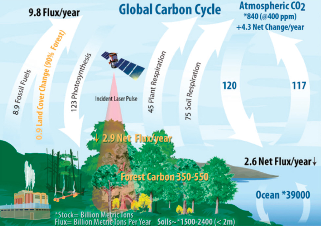
Together, climate and ecology help to determine biodiversity. This coupling, through biogeochemistry and the carbon cycle, affects greenhouse gas concentrations in the atmosphere, which in turn control ocean and land temperatures and affect essential vertical mixing in the ocean. Carbon moves through terrestrial ecosystems and oceans, exists in the atmosphere as gases including carbon dioxide (CO2) and methane (CH4), and exists in ocean water as inorganic carbon, in plankton, and in marine sediments (Figure 8.1). Since 1900 the atmospheric CO2 concentration has increased from 300 ppm to >400 ppm and continues to increase at the rate of approximately 2 ppm/year due to fossil fuel combustion and land use change. Global, budget-based analyses demonstrate that atmospheric CO2 concentrations would be further elevated if not for significant carbon uptake by terrestrial vegetation and the oceans, which together absorb nearly half of CO2 emissions (Khatiwala et al., 2009; Le Quéré et al., 2014).
___________________
2 See The World Bank, “World Development Indicators (2017). Agriculture, Value Added (Current US$).” https://data.worldbank.org/indicator/NV.AGR.TOTL.CN?end=2015&locations=US&start=1997&view=chart.
The concentrations of greenhouse gases control temperature, and in turn, directly affect ecosystem health, biodiversity, and the processes that influence carbon cycling. The deep ocean has also played an important role as a heat reservoir, mitigating the impact on lower atmosphere, land, and upper ocean temperatures (Rhein et al., 2013; Drijfhout et al., 2014). These fundamental linkages couple biogeochemistry, ecology, and biodiversity and will determine how climate and biodiversity change together in the future (Sommer et al., 2010; Harrison and Noss, 2017).
Intrinsic connections between ecosystems and the physical climate system also demonstrate the vulnerability of these key resources. For example, soil respiration increases with temperature, resulting in greater releases of CO2 during warm periods. Thawing of permafrost soils may release large amounts of CO2 and CH4 to the atmosphere. Changing patterns of upper ocean stratification due to warming and changing patterns of rainfall alter nutrient fluxes to the upper ocean, leading to changes in both concentration and ratios of essential nutrients that lead to shifts in community composition (Falkowski et al., 1998; Lomas
et al., 2014). Many of the benefits that society derives from ecosystems are related to the abundance and variety of life, but a deeper understanding of the processes governing ecosystem health is necessary. How will ecosystem diversity and productivity change with climate and with increased human demands for food? How will these changes affect the ecology and biogeochemistry of terrestrial, coastal, and open ocean habitats? What strategies can be implemented for the effective conservation and sustainable use of resources, including commercial fisheries and agriculture? Will land and ocean carbon reservoirs continue to absorb half of human CO2 emissions? And if not, what are the consequences for climate?
Satellite and in situ observations are fundamental to understanding the complex linkages between carbon, energy fluxes, and biodiversity. Only satellite-borne sensors can provide simultaneous global carbon cycle observations needed for quantifying large-scale carbon cycle processes that control the land’s forest and vegetation biomass stocks, and only satellite-borne sensors provide the necessary spatial and temporal observations to understand the role of the oceans in carbon fluxes and storage. Using data from these sensors with models now enables researchers to track carbon through the land, ocean, and atmosphere. As an observing system, satellites allow us to measure atmospheric CO2 and CH4, and estimate sources and sinks; measure land and ocean photosynthesis; measure the reservoir of carbon in plants on land and how this reservoir changes in space and time; and measure the extent and impact of fires and land use change.
In situ observations are necessary complements to satellite observations for confirming satellite-measured CO2 concentrations and determining soil and vegetation carbon quantities. In situ observations are also required to confirm the relationships between components of ocean ecosystems and ocean biogeochemistry, as well as the relationships between ocean carbon concentrations and observations derived from satellite radiances, and to provide critical vertical information. Atmospheric in situ observations of greenhouse gases are used to calibrate and validate satellite measurements and to refine atmospheric transport models, and provide critical multidecadal context needed to interpret observed variability.
A major challenge in addressing the dominant influence of temperature on ecosystems is capturing the movement of carbon, and hence feedbacks, between the multiple reservoirs—the atmosphere, terrestrial vegetation, soils, freshwater, oceans, and geological sediments—that collectively form the carbon cycle. Doing so requires that individual component fluxes be known to comparable levels of uncertainty (see Figure 8.1; Table 8.3). Consequently, a number of geophysical parameters are necessary for understanding the carbon cycle, and must be observed simultaneously: atmospheric CO2 and CH4 concentrations, land and ocean photosynthesis, land respiration and decomposition, and air-sea exchange. Also necessary are continuous measurements of processes that change at time scales of annual to decadal periods such as vegetation biomass, disturbance, and recovery, biomass burning, and carbon flux to the deep ocean.
Challenges, Opportunities, and Benefits of Prior Efforts
Challenges
Scaling
Ecosystems are complex, with species interacting at different trophic levels and different food webs that define the functional, structural, and biotic attributes of the system. Over different time scales disturbance forces create both rapid and slow changes, which cause significant and profound changes in ecosystem composition and function. Consequently, ecosystems have processes and functions that operate over different spatial and temporal scales and respond differently to different parts of the electromagnetic spectrum, depending on the conditions of the environment and the composition of the biosphere. The spatial resolution of an observation of an ecosystem is one of the important scales to understand to correctly interpret the spectral information. This problem is challenging when applied to ecosystems and biodiversity, as
TABLE 8.3 Current Flux Uncertainty Levels for the Land Carbon Cycle
| Carbon Cycle Component | Flux Uncertainty Now (Pg C and Atmospheric ppm CO2 Equivalent) | Reference |
|---|---|---|
| Atmospheric CO2 concentrations | ±0.1 Pg C or ±0.05 ppm CO2 | Tans and Thoning (2008) |
| Land gross primary productivity | ±8 Pg C or ±3.8 CO2 | Beer et al. (2010) |
| Vegetation disturbance and recovery | ±1 Pg C or ±0.5 ppm CO2 | Le Quéré et al. (2015) |
| Biomass burning | ±0.4 Pg C or ±0.2 ppm CO2 | van der Werf (2010) |
| Plant respiration | ±9 Pg C or ±4 ppm CO2 | Schlesinger and Bernhardt (2013) |
| Soil (roots, mycorrhizae, etc.) respiration-decomposition | ±15 Pg C or ±7 ppm CO2 | Schlesinger and Bernhardt (2013) |
NOTE: All fluxes are per year (see Figure 8.1). The current global land carbon sink is 2.9 Pg C/year with a land cover change flux of 0.9 Pg/C year. SOURCE: Data are from Tans and Thoning (2008); Le Quéré et al. (2015); Schlesinger and Bernhardt (2013); Beer et al. (2010); and van der Werf et al. (2013).
remote sensing technologies operate at specific scales. If the object is significantly smaller than the pixel or the process occurs at scales smaller than a pixel, it introduces uncertainty into the measurement. There are several approaches to addressing this problem: higher spatial resolution data can be used to train a classifier or validate results in coarser spatial data; statistical methods such as spectral mixture analysis can estimate the subpixel fraction of each component (endmember); and new computational statistical methods based on data analytics and machine learning can be used to solve subpixel composition.
Satellites with coarse resolution imagers include weather satellites having Geostationary Operational Environmental Satellite (GOES) or Polar Operational Environmental Satellites (POES) resolution at approximately 250 m to 1 km pixels—examples in the POR are VIIRS, NOAA-16, and PACE when it is launched. Moderate-resolution satellite imagers are generally in a polar orbit except for those on the ISS, which is in a 51-degree inclination orbit, allowing them to view the part of Earth under the satellite at different times of the day on different orbits. Moderate-resolution Landsat class satellites have pixel sizes that range from 10 m to 100 m. Examples are Landsat-7 and -8, Sentinel-2 and SPOT-4 and -5, and the proposed Earth observing satellites in the POR that are under construction, such as Environmental Mapping and Analysis Program (EnMAP), and for deployment on the ISS, such as ECOSTRESS and HISUI. Last, high spatial resolution polar-orbiting satellites that have smaller than 5 m pixel size are in the domain of commercial vendors. These are polar-orbiting multispectral satellites with very high spatial resolution, such as WorldView-1, -2, -3, and -4, Quickbird, GeoEye, and others. The company Planet is proposing to provide daily 5 m visible and near-infrared imagery from a large number of 3 Unit (3U) CubeSats. Still, the relative resolution (high, moderate, or coarse) may vary by application.
Improving Coverage in Key Regions
Understanding the function of ecosystems in high-latitude and tropical regions is critical for understanding the response of the Earth system to natural and human-induced changes. Northern hemisphere high latitudes have experienced the most warming during the past century resulting in an increase in growing season length and vegetation photosynthetic capacity. The impacts of increasing fire frequency, thawing of carbon-rich permafrost soils, melting sea ice, and changes in Southern Ocean circulation on ecosystems and carbon balance are unknown. Tropical ecosystems support the greatest biodiversity and largest carbon stocks on the planet, but these dense and sparsely inhabited areas are critically undersampled by in situ networks. Both high-latitude and tropical ecosystems are challenging to observe by satellite because of persistent cloudiness and a lack of ground-based calibration/validation resources. However, improvements over current generation satellites are possible through the expanded use of lidar and Synthetic Aperture Radar (SAR)—for example, the European Space Agency (ESA) Sentinel-1a and -1b missions—technologies, increased sampling frequency by combining information from multiple sensors, and expanded airborne and ground-based sampling. An excellent example of this is the harmonization of Landsat-8, Sentinel-2a, and Sentinel-2b 30 m multispectral data with an equatorial revisit frequency of 3.7 days.
Data Services
Increasing spatial and temporal resolution of satellite data products, including those from the commercial sector, enables significant advances in ecosystem science, but poses a challenge for both data providers and users. Advanced visualization, data subsetting, and remote access tools can aid users, especially those without science or computational backgrounds, but require sustained support by funding agencies.
Opportunities
Leveraging Sustained Land Imaging
International investments in sustained land imaging now provide global 30 m multispectral imagery at an equatorial repeat frequency of 3.7 days, with an increase in sampling frequency to 3 days anticipated in 2020 with the launch of Landsat-9. This capability will lead to improving observation-based estimates of gross primary production (GPP) and other carbon fluxes that have previously used MODIS data at 1 km resolution (Badgley et al., 2017). Continuity of these critical long-term data sets provides a crucial context for new measurements that will enable a deeper understanding of ecosystem function and structure. These data could be enhanced by the addition of hyperspectral data that can provide additional information on ecosystem functioning.
Transitioning Mature Airborne Technology to Space
Following the 2007 Earth Science Decadal Survey, NASA made substantial technology investments in airborne hyperspectral imaging of vegetation and ocean color, and lidar observations of vegetation structure, greenhouse gases, and ocean profiles of particulate carbon. These technologies have been demonstrated by aircraft, supporting more rapid development and deployment of such missions.
Synergy with Commercial Satellite Data
The commercial sector is actively developing small satellite systems for Earth imaging. For example, Planet uses off-the-shelf electronics to build highly capable small satellites launched into constellations that will have the capability to image Earth daily. Capella Space is developing small satellites to provide SAR imagery from constellations of small satellites. The potential for measuring the OCR of coastal waters
from small satellites will be evaluated by SeaHawk,3 a proof-of-concept mission supported by the Moore Foundation. Small satellites have significant potential to cut launch and other costs, although their capability to meet science community objectives needs to be demonstrated. The panel also notes that to meet these objectives, small satellites are reliant on the calibration and mapping integrity provided by Landsat and other medium-resolution satellites.
Benefits of Prior Efforts
Satellite observations over the past several decades have enabled routine monitoring of global ecosystems and a better understanding of their interaction with climate and human-induced change (NRC, 2008). Quantifying primary production for both terrestrial and marine ecosystems has been a central concern of carbon cycle research and is now integrated into earth system models.
Accurate estimates of leaf area index (LAI) are critical to correctly scaling carbon, water, and energy fluxes to estimate rates of photosynthesis, evapotranspiration, and respiration on land surfaces. Today, MODIS and VIIRS provide accurate estimates of LAI that inform global estimates of terrestrial GPP and NPP, and, combined with the AVHRR/2 time series (in operation since 1981), provide a multidecadal record of how ecosystems have changed. Recent work has shown that satellite observations of solar-induced fluorescence (SIF) from atmospheric composition satellites (OCO-2, GOSAT, GOME-2) can identify periods when vegetative productivity is low (e.g., Frankenberg et al., 2011; Joiner et al., 2011) and have been combined with MODIS multispectral imagery to produce GPP estimates entirely from observations (Badgley et al., 2017).
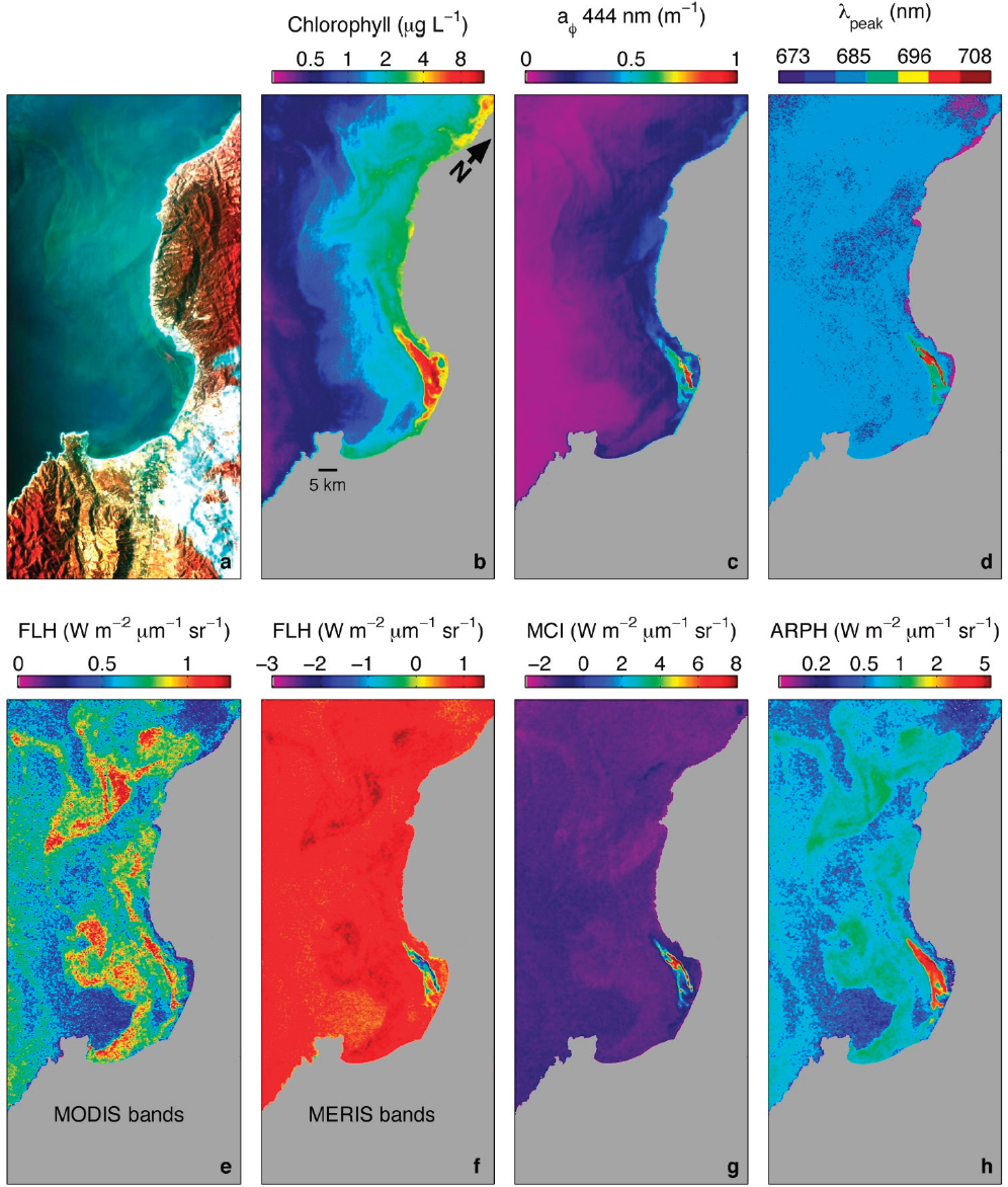
Satellite ocean color measurements have proven to be essential for supporting the science and applications related to ocean ecosystems and biogeochemistry. These and other ancillary measurements (e.g., incident solar irradiance) are used to calculate the mean and fluctuating components of ocean NPP at regional to global scales. Additional spectral bands of NASA’s MODIS and ESA’s medium-spectral resolution imaging spectrometer (MERIS) were also used to estimate ecological parameters such as phytoplankton size and taxonomic composition, both of which affect the efficiency of carbon flow from phytoplankton to higher trophic levels, including fish, and to the long-term sequestration of exported carbon in the ocean interior. For MODIS additional narrow-band measurements around the chlorophyll-a fluorescence peak at 685 nm added the potential for estimating the physiological state of phytoplankton and its growth potential. The PACE mission will enable a significant leap forward in our ability to quantify seawater components and how their distributions change and respond to the physics and chemistry of the ocean.
Satellite data have also revolutionized our understanding of how humans use and change the landscape, which has implications for the structure and functioning of ecosystems, and their exchanges of energy, water, and nutrients. Obtaining global land cover maps has been a goal of terrestrial remote sensing from the beginning of Landsat; however, only since the EOS era have direct measurements of land cover been produced at an appropriate global scale (DeFries and Townshend, 1999). Landsat data with its 30 m spatial resolution and consistent, long-term sampling provides an excellent data set that has been used to assess changes in global forests (e.g., Hansen et al., 2013) and climatic shifts in high-latitude ecosystems (e.g., Ju and Masek, 2016). These data sets have also supported widespread monitoring of agricultural production. The use of Landsat, MODIS, and VIIRS satellite data is central to global projects including the Famine Early Warning System Network established by the U.S. Agency for International Development (USAID) in 1985 and the U.S. Department of Agriculture’s (USDA’s) global agricultural production estimates released monthly (USDA, 2017). As extensive observational data from Landsat, Sentinel-2, and commercial
___________________
3 See University of North Carolina, Wilmington, “SOCON: Sustained Ocean Color Observations with Nanosatellites: SeaHawk CubeSat Satellite Bus,” http://uncwweb.uncw.edu/socon/seahawk.html.
satellites become increasingly available, along with ancillary data in relational geospatial databases, they support informatics approaches that aid farmers in optimizing yields (Liu et al., 2010; Zheng et al., 2013; Verrelst et al., 2014; Guan et al., 2017; Veloso et al., 2017).
The same data sets have also provided the best global source of information regarding the impact of fires on ecosystems. For example, early studies with AVHRR showed that most fires in the tropics are of anthropogenic origin, while in the boreal forests, large wildfires were generally caused by lightning (Verbesselt et al., 2012). More recently, analysis of MODIS and VIIRS data provided refined estimates of burned area and of emissions of trace gases and aerosols from fires (e.g., van der Werf et al., 2006, 2010; Schroeder et al., 2014).
Airborne observations have been used to document wildfire temperatures by measuring the enhanced radiance in the hyperspectral SWIR bands (e.g., Dennison et al., 2006) and have documented the progressive drought stress in California’s forest ecosystems in 2012-2015 using NIR water absorption bands (Asner et al., 2016b). Hyperspectral imagery is expected to improve understanding of the physiological responses of vegetation to these and other environmental disturbances (Khanna et al., 2013; Kefauver et al., 2014; Sanches et al., 2014). However, this potential has been poorly documented given the lack of satellite-based observations other than Hyperion, a one-year demonstration project launched in 2000, which lacked adequate signal-to-noise ratios for use in aquatic systems and many terrestrial applications. Despite its limitations Hyperion has demonstrated the potential for hyperspectral data compared to multispectral systems (Marshall and Thenkaball, 2015), and provides the basis for algorithms applicable to next-generation sensors such as EnMAP and Hyperspectral Infrared Imager (HyspIRI; e.g., Christian et al., 2015; Zhang et al., 2016).
Satellite and aircraft remote sensing observations have also greatly improved our understanding of coastal, wetland, estuarine, coral reef, and inland aquatic ecosystems. For example, airborne hyperspectral observations can be used to classify coral reef cover types (Hochberg and Atkinson, 2000) and estimate primary production rates and distributions (Hochberg and Atkinson, 2008). Landsat-5 imagery was used to construct a 30+ year time series of giant kelp canopy biomass on a 30 m basis over the entire California coastal waters and was used to diagnose the controls on kelp canopy changes in space and time (e.g., Bell et al., 2015a). Hyperspectral Airborne Visible and Infrared Imaging Spectrometer (AVIRIS) airborne observations have extended this remote analysis of kelp forests by enabling the retrieval of kelp canopy chlorophyll concentrations independently from carbon biomass, providing robust proxies of the photo-physiological state of the kelp forests (Bell et al., 2015b). Last, high-resolution airborne imagery was used to assess seagrass cover and water depth of the Bahamas Banks (Dierssen et al., 2003). The airborne results cited here demonstrate the capabilities that hyperspectral remote sensing brings to understanding terrestrial, coastal, and aquatic ecosystems. While Hyperion was not widely used for aquatic systems, the Hyperspectral Imager for the Coastal Ocean (HICO) sensor aboard the International Space Station provides another example of how hyperspectral information would improve understanding of aquatic systems compared to multispectral systems (Ryan et al., 2011; Figure 8.2).
PRIORITIZED SCIENCE OBJECTIVES AND ENABLING MEASUREMENTS
This panel identified five overarching science questions within three primary topic areas that remote sensing can contribute to in the coming decade. Those broad topic areas are (1) structure, function, and biodiversity; (2) fluxes of carbon, water, nutrients, and energy; and (3) carbon accounting. For each of the science questions, the panel further identified several objectives. The five questions are enumerated in the following sections with the associated objectives described in detail. The panel recognized all objectives as being important, but notes those that are Very Important (Objective E-1a) and Most Important (Objectives E-1b, E-1c, E-2a, and E-3a).
E-1: Ecosystem Structure, Function, and Biodiversity
Question E-1. What are the structure, function, and biodiversity of Earth’s ecosystems, and how and why are they changing in time and space? (“Structure” is the spatial distribution of plants and their components on land, and of aquatic biomass. “Function” is the physiology and underpinning of biophysical and biogeochemical properties of terrestrial vegetation and shallow aquatic vegetation.)
Objective E-1a
Objective E-1a. Quantify the distribution of the functional traits, functional types, and composition of terrestrial and shallow aquatic vegetation and marine biomass, spatially and over time.
Motivation
Characterization of the functional traits, functional types, and composition of terrestrial vegetation was identified by the Ecosystems Panel as a Very Important measurement based on the need to better understand the relationships between the composition of the biosphere and other Earth system processes, including climate. Multiple properties of plants (biochemistry, structure, phenology, reproduction) determine their ecological role in the biosphere. The collection of these plant properties embodies the taxonomic composition, abundance, and biomass, and their variations in space and over time defines their role in both terrestrial and marine ecosystems. These plant properties determine the patterns of energy, carbon, water, and nutrient fluxes for these systems (Lavorel et al., 2002; Diaz et al., 2004; Kattge et al., 2011; Asner et al., 2016a). It is now feasible, given hyperspectral imaging instrumentation, to map the distribution and concentrations of many terrestrial canopy biochemical and structural properties from space, which will provide new opportunities to monitor and quantify ecosystem composition and function (Schimel et al., 2013; Jetz et al., 2016; Asner et al., 2017). Hyperspectral imaging affords the most accurate community structure mapping in shallow marine systems, such as coral reefs (Hochberg et al., 2003; Hedley, 2013). Identifying taxonomic composition does not necessarily imply a specific rank like genus and species, as it can also apply to the family level or the conifer clade within the gymnosperms. This panel does not advocate for a requirement to identify and map all 300,000 or so terrestrial and aquatic plant species but instead notes that newer hyperspectral technologies can increase our understanding of the most abundant or dominant species in Earth’s ecosystems as measured from space at a Landsat-class spatial resolution. For example, consider a gradient in water availability across a deciduous hardwood forest that may be observed in the field as a change in the distribution of deciduous hardwood species across the gradient, but this compositional change would not be detected from orbit with existing technology, as there would be no change in the “functional type” of the ecosystem as currently mapped. Mapping at the taxonomic level using imaging spectrometry has advanced rapidly in all types of environments in the past two decades, from Roberts et al. (1998) and Underwood et al. (2003) to Ferreira et al. (2016), Laurin et al. (2016), and Roth et al. (2016), but the level of species resolution depends on the traits that distinguish one species (or genera, family, or clade) relative to others in their surroundings. There are a growing number of papers that show relationships between plant biodiversity (and its relation to heterotrophic biodiversity) and spectral characteristics. In some cases species, subspecies, or subgenera are defined (Cavender-Bares et al., 2016); in others, emphasis is on alpha, beta, or gamma diversity without specifying species composition (Punalekar et al, 2016; Wang et al. 2016a, 2016b). Expanding our knowledge of the composition of terrestrial ecosystems is also important for modeling habitat suitability for all species including animals, many of which have critical land and water conservation monitoring needs. Doing so also forms a bridge between species (and their functioning) and the rest of the Earth system.
Similar to terrestrial systems, understanding biodiversity in aquatic ecosystems in relation to biogeochemical cycles requires quantification of the functional composition and changes over appropriate temporal and spatial scales. Appropriate scales are question-dependent, but for coastal aquatic systems, a commonly cited requirement is to achieve subtidal (hours) temporal revisit rates, with spatial resolutions between 10-200 m (Devred et al., 2013; Mouw et al., 2015; Moses et al., 2016). Aquatic ecosystems have many important roles in the global system. For example, the oceans support highly productive and diverse ecosystems that have important roles in the global cycling of carbon and the sequestration of CO2 on monthly to millennial time scales. Coastal ocean, brackish water, and freshwater ecosystems provide a wide range of ecosystem services to society, from critical habitats for endangered species, to coastal protection, to fisheries. For planktonic ecosystems, functional types can be defined in terms of the cell size and biogeochemical roles of the phytoplankton populations, as a function of food quality for higher trophic levels, and as beneficial versus harmful algal bloom (HAB) groups.
For many marine faunal species, population characteristics are defined by habitat suitability mapping, which in turn, often requires continuous mapping of NPP and other parameters. Faunal suitability mapping is particularly important for conservation and fisheries applications. Hence, the characterization of oceanic, coastal, and freshwater aquatic ecosystems requires a taxonomic or functional characterization of the composition of these systems obtained from satellite observations. This is important, because ecosystem structure affects the efficiency of energy transfer through marine food webs, ultimately determining fish production and the flux of organic matter into deeper ocean waters. High spectral resolution measurements from PACE (1 km) and from a future high spatial resolution (30 m) imaging spectrometer for coastal and inland waters will determine signatures of phytoplankton taxonomic diversity and particle size distributions, enabling us for the first time to quantify global ocean ecosystem structure and biodiversity metrics from space. Space-based high-resolution imaging spectroscopy will also enable for the first time global characterization of the nearshore coastal zone and shallow aquatic ecosystems.
The wide array and inherent accuracy of the observables will provide critically needed support for developing and validating numerical models linking biology and physics to forecast future ocean ecosystem structure and the ocean carbon cycling they regulate.
Measurement Objectives
The suite of land plant properties observable by satellite sensors are those that absorb and reflect energy in the wavelengths between the visible and shortwave infrared region of the solar spectrum (400-2500 nm). Because these measurements relate to observations of photosynthetic pigments, water content, carbon concentrations, nutrients, and other biochemicals that are related to plant productivity, structure, and defense, they provide direct information about ecosystem function. Measurements and use of such traits to infer functional processes has a long history in the plant biology and ecological literature and more recently in the development of large plant trait databases, such as the TRY database (Kattge et al., 2011). Imaging spectrometer measurements and analysis from NASA’s AVIRIS and numerous other imaging spectrometers have been widely published throughout the remote sensing literature. While there are no “standard products” for AVIRIS because it is a research instrument, the HyspIRI Airborne Preparatory Project developed a set of georectified and atmospherically corrected radiance products to simulate data flow from an operational hyperspectral satellite. Case studies and products enabled by next-generation remote sensing were highlighted in a recent special issue.4
___________________
4 See Remote Sensing of Environment, 2015, “Special Issue on the Hyperspectral Infrared Imager (HyspIRI): Emerging Science in Terrestrial and Aquatic Ecology, Radiation Balance and Hazards,” Volume 167, https://doi.org/10.1016/j.rse.2015.06.011.
In 10 years of mapping the functional diversity of tropical and temperate forest canopy species, a large literature has developed on the use of imaging spectroscopy to map plant functional types, tree species diversity, and their biochemical traits (Kokaly, 2001; Kokaly et al., 2009; Clevers et al., 2011; Asner et al., 2014; Cheng et al., 2014; Féret and Asner, 2014, 2015; Sebrin et al., 2014; Asner and Martin, 2016; Meerdink et al., 2016).
There is a recognized need to improve estimates of photosynthetic and respiratory responses to light and temperature to increase accuracy of estimates of GPP, NPP, and Net Ecosystem Productivity (NEP). In particular, improving parameters related to nitrogen content, SIF, Vcmax, and Jmax, are important to improving today’s Earth system models (Rogers et al., 2017). This is an active area of photosynthetic research, and there are recent papers that support the relationship between leaf nitrogen concentration and Vcmax and Jmax (Dechant et al., 2017; Kattge et al., 2009; Quebbeman and Ramirez, 2016). Quebbeman and Ramirez (2016) approached modeling from a mechanistic optimization perspective and tested it with data from the TRY database (Kattge et al., 2011), while Dechant et al. (2017) empirically found relationships through canopy measurements. Numerous papers (e.g., Kokaly et al., 2009; Clevers et al., 2011; Serbin et al., 2014; Meerdink et al., 2016) show good quantitative predictions of leaf nitrogen from leaf, canopy, and imaging reflectance levels. Given the significance of these measurements of photosynthetic performance, this research could yield significant advances from imaging spectroscopy that would increase our ability to better measure GPP, including measurements of SIF. The scientific and applications benefits of measuring GPP from space using solar-induced fluorescence would also advance our understanding of the carbon cycle (Badgley et al., 2017).
Spaceborne imaging spectrometer data are needed over large areas to measure ecosystem composition and plant functional properties of land vegetation. Airborne imaging spectroscopy in the visible to shortwave infrared (VSWIR) spectral region has demonstrated the ability to acquire this critical information over large spatial domains (meters to thousands of kilometers), while SLI provides phenology observations every 4 days (Richardson et al., 2012). The capacity to monitor and follow changes in functional traits and functional types and observe vegetation phenology at a 30 m spatial resolution from Earth orbit will transform our ability to understand and predict future changes in ecosystems that result from land use, disturbance, severe weather, and climate changes. While imaging spectroscopy is the only technology that can provide the detailed spectral data to allow identification and quantification of major biochemical and structural components of plant canopies, the combination of hyperspectral imagery with multispectral time series data will achieve improved understanding of ecosystem function and early detection of changes in these processes. In support of such a mission, NASA has invested in numerous pre-HyspIRI airborne, modeling, and field program activities, with numerous publications and government documentation, to further advance and mature the coupled science and technology for a future orbital spaceborne imaging spectrometer mission. NASA, the U.S. Geological Survey (USGS), and ESA are now merging or harmonizing Landsat-8, Sentinel-2a, and Sentinel-2b 30 m multispectral imagery with an equatorial repeat frequency of 3.7 days.
Within aquatic systems a suite of biogeochemical traits can also be inferred from spectral radiometry based on a combination of structure (cell size and particulate inorganic and organic carbon), pigments (to identify functional groups of algae), and discrete fluorescence bands to assess physiology (e.g., Devred et al., 2013; Mouw et al., 2015; Moses et al., 2016). Analogous to terrestrial remote sensing, this information can be used to identify harmful algal blooms and partition total biomass into size classes, providing information about trophic transfer and export flux (e.g., Uitz et al., 2010; Siegel et al., 2014; Mouw et al., 2015). In some cases remote sensing observations can be used to infer physiological status—for example, by estimating the carbon:chlorophyll ratio of phytoplankton populations (Behrenfeld et al., 2005) and giant kelp forest canopies (Bell et al., 2015b). As with terrestrial remote sensing, the capacity to track changes
in these processes has the potential to transform our ability to understand and predict future changes in ecosystems resulting from resource management, disturbance, annual to decadal oscillations (e.g., El Niño), and climate change. While some of these traits could be obtained from multispectral imagery, a targeted coastal imaging sensor is necessary to achieve all of the goals, and is complementary with similar efforts for the open ocean using PACE and consistent with suggestions for a terrestrial hyperspectral imaging sensor.
For shallow seafloor systems, such as coral reefs, current aspirations are more modest. Ecosystem structural and functional features are more similar to those of terrestrial systems than to those of the open ocean, but strong absorption of red and NIR wavelengths by water largely precludes direct sensing of detailed biochemical and physiological parameters. Pigmentation has been demonstrated to be retrievable via hyperspectral measurements at the level of the coral colony (Hochberg et al., 2006), but it is unknown how such observations might scale to larger remote sensing pixels, although progress has been made in that direction for giant kelp (Bell et al., 2015b). In general though, the main objective is identification and quantification of basic benthic community structure—for example, for coral reefs, the proportional cover of coral, algae, and sand (Hochberg, 2011). Owing to the complexity of light interactions in these environments, high to moderate spatial resolution imaging spectroscopy has been demonstrated to provide greater retrieval accuracy than multispectral sensors (e.g., Botha et al., 2013; Phinn et al., 2013).
Measurement Approaches
Three measurement systems are required to quantify the composition of terrestrial vegetation and marine biomass. First, a moderate spatial resolution (30-45 m Ground Sample Distance [GSD]), hyperspectral resolution (10 nm; 400-2500 nm), high fidelity (Signal to Noise Ratio [SNR] = 400:1 Visible and Near Infrared [VNIR]/250:1 Short-wave Infrared [SWIR]) imaging spectrometer is needed for characterizing land, inland aquatic, coastal zone, and shallow coral reef ecosystems (possibly with commonality to an implementation of TO-18 in Appendix C, the Surface Biology and Geology Targeted Observable; this corresponds to the region in Figure 8.3 referred to as HyspIRI).
Second, a global ocean color mission (GSD = 0.25-1.0 km; revisit ≤ 2 days) is required to properly assess open ocean planktonic ecosystems. Its sensor should be hyperspectral ocean (5 nm; 380-1050 nm) with high fidelity (SNR ≥ 1000:1 at Top of Atmosphere [TOA] clear sky ocean radiance) so that phytoplank-
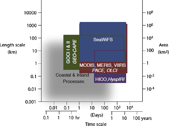
ton NPP processes and functional types can be quantified in challenging environments. The successful launch of the PACE mission in NASA’s Program of Record would satisfy this need.
Last, there remains a need for moderate-spatial (~250 m), high-temporal (2-3 hour repeat), hyperspectral (5-10 nm; 380-1050 nm) observations for coastal and inland waters (Figure 8.3; TO-3 in Appendix C, the Aquatic-Coastal Biochemistry Targeted Observable), particularly for the western hemisphere (Corson et al., 2011; Fishman et al., 2012; Pahlevan et al., 2014; Arnone et al., 2016). This can be achieved via geostationary orbits or via a constellation of small satellites with orbits optimized to cover priority coastal waters (e.g., U.S. coastal waters). SeaHawk is a proof-of-concept mission based on a small satellite program and will provide the first operational test case for use of a constellation of small satellites targeting OCR. While the spectral resolution is limited (based on the legacy SeaWiFS sensor), the SeaHawk concept provides an important opportunity to evaluate the improved spatial coverage for coastal and inland waters.
Objective E-1b
Objective E-1b. Quantify the global three-dimensional (3D) structure of terrestrial vegetation and 3D distribution of marine planktonic biomass within the euphotic zone, spatially and over time.
Motivation
Quantifying the global 3D structure of terrestrial vegetation and marine planktonic biomass within the euphotic zone, spatially and over time, was identified as among a few objectives ranked as Most Important. Measurements of the 3D physical structure of vegetation are a priority, because canopy height profiles and aboveground biomass, particularly in forested ecosystems of the world, have a wide range of practical applications. Forest carbon stock estimates, based on calibration and validation of canopy structure metrics (profiles of canopy elements) with forest inventory measurements, provide robust “emission factor” data that, when coupled with “activity data” associated with changes in forest cover and extent, form the basis for emissions reporting, including uncertainties, using standard protocols (Tyukavina et al., 2015; Goetz et al., 2016).
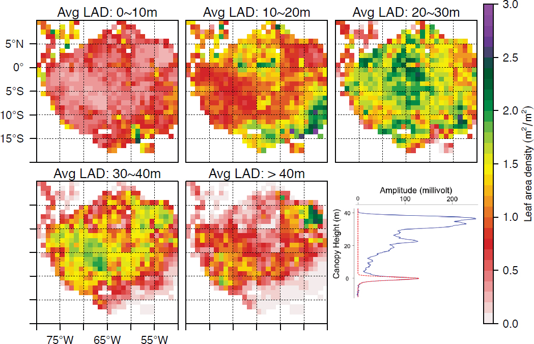
Mapping forest structure and carbon stocks is widely used in forest management (Dubayah et al., 2010; Wulder et al., 2012) and highly relevant to safeguarding the livelihoods of communities dependent on forests for fuel, fiber, and food (“provisioning” ecosystem services). Most recently, lidar-derived forest structure measurements have helped to resolve long-standing debates about the influence of drought on tropical forest productivity and variability (Tang and Dubayah, 2017; see Figure 8.4). Forest structure metrics are also well-documented determinants of animal habitat properties, and thus community abundance and biological diversity, as well as habitat preferences and utilization (reviewed by Lefsky et al., 2002; Vierling et al., 2008; Bergen et al., 2009; Davies and Asner, 2014). The latter, in turn, is important for biodiversity conservation and adaptive management of threatened and endangered species (Goetz et al., 2010).
Quantification of the vertical dimension of marine biomass has long eluded satellite oceanographers. In order to measure global stocks of planktonic biomass, knowledge of the vertical dimension of biomass is required. Many studies assume that phytoplankton biomass levels are uniform throughout the euphotic zone (Behrenfeld et al., 2006, 2013; Siegel et al., 2014), although this clearly is not a valid assumption. Understanding the vertical profile of ocean biomass on global scales will greatly improve satellite retrievals of NPP rates as well as provide determinations of mixed layer euphotic zone depths. Recent results from NASA’s Ship-Aircraft Bio-Optical Research (SABOR) field campaign showed substantial improvements in NPP estimates (up to 54 percent) when lidar-derived profiles of optical properties are used (Schulien et al., 2017). BioArgo floats will provide vertical profiles of ocean temperature and salinity, as well as biological parameters, dissolved oxygen, and backscatter much deeper into the water column than the lidar profiles.
However, the upper ocean part of the BioArgo profile will overlap with the lidar measurements, and thus provide complementary measurements for comparisons and calibrations.
Unlike satellite ocean color imagers, active remote sensing with lidars can operate during darkness and can penetrate through moderate cloud and aerosol layers. This is critical for very high latitude oceans where the complete annual coverage of phytoplankton biomass is poorly known (Behrenfeld et al., 2017). The ability of advanced lidars to profile up to three optical depths also makes them useful for understanding ocean biological processes under perpetually cloudy conditions, such as the sub-Arctic North Pacific Ocean. Understanding ocean ecosystem processes in the Arctic Ocean and throughout the Southern Ocean is critical, as these ecosystems are changing rapidly due to warming and altered circulation patterns (Smetacek and Nicol, 2005; Schofield et al., 2010).
Measurement Objectives
A lidar satellite mission to provide 3D vegetation structure has long been a high priority of the terrestrial ecosystem science community, with a history dating back to the canceled Vegetation Canopy Lidar (VCL) mission in the mid-1990s; the Deformation, Ecosystem Structure, and Dynamics of Ice (DESDynI) mission called for by the 2007 decadal survey but canceled as a result of budget shortfalls during the 2007-2009 financial crisis; and most recently the Global Ecosystem Dynamics Investigation (GEDI) lidar planned for a 2-year deployment on the International Space Station (ISS) by early 2019. Prior science definition teams of VCL, DESDynI-LiDAR, and GEDI-LiDAR have all specified measurement criteria that meet well-defined science needs. These have been extensively documented in NASA reports (DESDynI workshop report, 2007) and peer-reviewed publications.
GEDI-LiDAR, as the first space-based 1064 nm waveform lidar designed for ecosystem studies, will substantially advance mapping of forest canopy 3D structure and aboveground biomass for areas between ±52 degrees latitude. With full waveform sampling using multiple lasers that produce a 25 m footprint at the surface, GEDI is an appropriate model for next-decade ecosystem characterization with lidar. Desired sampling for ecosystem studies include 1 ha cells populated with 10-25 m footprint acquisitions, with global scale repeat sampling every 5 years.
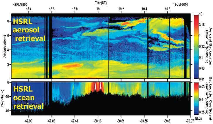
Airborne and shipborne lidars generally measuring at 532 nm have long been used to quantify a variety of aquatic science problems, from the assessment of internal wave propagation on subsurface particle maxima to marine fish schooling (e.g., Churnside, 2014). The Cloud-Aerosol Lidar with Orthogonal Polarization (CALIOP) satellite mission enabled an average of relevant oceanographic optical properties through the upper ocean to depths of 10s of meters (Behrenfeld et al., 2017). Lidars are active, so they can be deployed at night and provide observations in regions with zero or very low sun elevations where passive ocean color sensors do not provide data. Advanced lidars, such as the High Spectral Resolution Lidar (HSRL; Piironen and Eloranta, 1994; Hair et al., 2008), determine vertical profiles of both aerosol and cloud particle backscattering coefficients as well as the lidar beam’s vertical attenuation in the ocean over several optical depths. The HSRL system has been extensively demonstrated in the field from aircraft (Hair et al., 2008; Müller et al., 2014; Burton, 2015; Schulien et al., 2017).
Understanding the vertical profile of ocean biomass on global scales will greatly improve satellite-based calculations of NPP, as well as determinations of mixed layer and euphotic zone depths. The utility of such measurements was demonstrated recently for polar waters with the spaceborne CALIOP lidar (Behrenfeld et al., 2017). Of the global ocean, polar regions, particularly the Arctic, are seeing the most rapid warming and other changes such as loss of sea-ice cover. These have as yet unknown impacts on polar ecosystems. Data from lidars simultaneously profiling backscatter and beam attenuation at 355 nm and 532 nm can provide measurements that can be related to particulate carbon concentrations and dissolved organic matter absorption.
CALIOP was not designed to make in-ocean retrievals and cannot retrieve vertical profiles on oceanic scales (Lu et al., 2014), and an advanced lidar with oceanic profiling capability has not yet been flown in space. However, advanced lidars, such as the HSRL, enable multiple ocean property profile retrievals through about three optical depths, and this capability has been recently demonstrated in the field from HSRL airborne missions for several NASA oceanographic field campaigns (SABOR; North Atlantic Aerosols and Marine Ecosystem Study [NAAMES]; Azores; see Figure 8.5).
An advanced lidar instrument using the HSRL 532 nm channel would represent a substantial increase in the quality of the vertically resolved measurements for oceanic and most other applications. Vertical profiles of particle backscatter and vertical lidar path attenuation are created and are related to the total seawater absorption coefficient. To first order, passive ocean color observations provide measurement of
the ratio of the backscatter to absorption coefficients, whereas advanced lidar instruments provide these optical properties separately (which will be useful in integrated passive-active ocean retrievals) in the form of a vertical profile. With two advanced lidar channels at 355 and 532 nm, information can be obtained about ocean particle size distributions and separation of phytoplankton from colored dissolved organic matter absorption coefficients (Bruneau et al., 2015).
Measurement Approaches
Terrestrial Vegetation Lidar
The measurement approach for this objective would consist of imaging waveform acquired in swaths, with desired sampling of 1 ha cells with 10-25 m footprint size and global sampling every 5 years at 1064 nm.
Synergistic uses of spaceborne lidar with other missions in the POR, as well as new missions, are multifold. The GEDI is a lidar for sampling canopy structure and biomass that will be hosted on the ISS in 2019 and will operate for 2 years. ICESat-2, although not ideal for land vegetation because its wavelength is 532 nm, will be launched in 2020. Other examples include synergy with the NASA-ISRO Synthetic Aperture Radar (NISAR) radar mission, which launches circa 2022, as well as with the ESA P-band BIOMASS mission (launch in 2021), providing opportunity to spatially extend the lidar sampling to map 3D structure more extensively and contemporaneously. This panel notes that the ESA P-band BIOMASS mission is not permitted to operate over some parts of the world (including the United States) because of the operation of comparable frequency radars for tracking objects in space. Synergy with a new imaging spectrometer would also confer significant advances in assessments of the carbon cycle (Schimel et al., 2015) and biodiversity conservation (Asner et al., 2017) in combination with sustained land imaging. Lidar would be also synergistic with the other ISS instruments (OCO-3, ECOSTRESS, and HISUI) and with the
Landsat-8, Landsat-9, Sentinel-2a, and Sentinel-2b satellite fleet that could incorporate structure metrics, including biomass, in assessments of forest disturbance and recovery change.
While past efforts have demonstrated this capability using ICESat-1 Geoscience Laser Altimeter System (GLAS) waveform lidar with MODIS imagery (Baccini et al., 2012; Saatchi et al., 2011), synergy with the ICESat-2 photon-counting lidar to launch in 2020 provides opportunities to extend GEDI 3D structure to higher latitudes. This will compensate for the ICESat-2 lidar 532 nm penetration limitations for retrieving structure information in moderate to higher biomass forested regions. Last, synergy of waveform lidar with digital surface models derived from high-resolution commercial satellite stereo imagery can be used to generate canopy structure maps, when calibrated with 3D structure measurements from GEDI and ICESat-2 lidars to derive maps of surface topography beneath the canopy. These synergies have benefits across the research priorities of the decadal survey panels.
Ocean Plankton Biomass Profiling Lidar
Profiling ocean-aerosol-cloud lidar like a multispectral HSRL-2 will have the capability to make profiles of ocean biospheric properties on global scales. The instrument should have ~2 m vertical resolution and the ability to determine profiles of particle backscatter and diffuse attenuation spectra through the upper three optical depths of the ocean. The profiling lidar should have ~1 km footprint and sampling along track with near nadir viewing. It would be best if the ocean lidar system was flown in a Sun synchronous orbit to enable rapid global coverage and synergies with passive ocean color instruments. Optimally, the ocean profiling lidar would have three laser wavelengths—1064, 532, and 355 nm—so that spectral properties of both particle backscatter and diffuse attenuation can be diagnosed. This would enable the determination of the shape of particle number size spectra from the spectral information and a partitioning of phytoplankton absorption properties from colored dissolved organic matter (CDOM) absorption. The 355 nm channel makes the partitioning of phytoplankton from CDOM absorption possible. The ocean profiling lidar will revolutionize satellite remote sensing of the global ocean even without the 355 nm channel. The ocean profiling lidar builds on the successes of retrieving ocean properties from the CALIOP lidar (e.g., Behrenfeld et al., 2017). A similar profiling lidar was included in the ACE mission concept from the last decadal survey. Further NASA development and implementation of airborne HSRL-2 lidar systems are presently used in several NASA field campaigns.
Objective E-1c
Objective E-1c. Quantify the physiological dynamics of terrestrial and aquatic primary producers.
Motivation
The panel identified quantification of the physiological dynamics of primary producers as another Most Important priority.
A key to understanding the biogeochemical cycles and fluxes discussed in Questions E-2 and E-3, their sensitivity to climate change, and their feedbacks to climate are predictions of future conditions of the biosphere and the climate system. The biochemical properties of terrestrial vegetation, aquatic biomass, and soils provide quantitative or qualitative measurements that are used to determine the physiological dynamics of primary producers and soil processes. Determining the full range of physiological dynamics by quantifying canopy chemistry related to these processes also contributes to determining the functional types and traits of terrestrial ecosystems (Objective E-1a) and to determining vegetative biodiversity (see Objective E-1e).
Ocean color radiometry can determine important characteristics of phytoplankton physiology, providing a better understanding of bulk marine NPP estimates. For example, Bell et al. (2015b) demonstrate that
giant kelp (macroalgae) physiological status can be assessed by directly estimating the carbon to chlorophyll ratio, and that it may be possible to estimate subtle changes in pigment ratios indicative of shifting environmental stressors and conditions. On a larger scale Behrenfeld et al. (2009) show that incorporation of fluorescence quantum yield characterizes nutrient (particularly iron) stress globally, while McGaraghan et al. (2011) demonstrate an ability to identify trends of iron bioavailability at high spatial and temporal resolution in the coastal ocean. These tools can identify shifts in physiological capacity that ultimately impact NPP, and therefore biogeochemical cycling. Quantification with an imaging spectrometer will also allow assessment of emergent properties related to the physiological dynamics of primary producers. For example, AVIRIS-Classic was used in San Francisco Bay to relate phytoplankton functional types to food quality, demonstrating that total biomass, or even growth rates, are inadequate for understanding how phytoplankton composition affects ecosystem function through trophic transfer (Kudela et al., 2016).
Measurement Objectives
The biochemical properties of terrestrial vegetation, aquatic (including ocean) biomass, and soils provide quantitative or qualitative measurements that are used to determine the physiological dynamics of primary producers and soil processes. Pigment composition can be used in both terrestrial and aquatic environments to quantify functional diversity.
For aquatic applications PACE in the POR for the open ocean and a high spatial resolution (30 m) hyperspectral sensor for coastal and inland waters will provide critical information on phytoplankton physiology and ecosystem health. The key to these observations is to complement higher spectral resolution observations in the blue to yellow wavelengths with very sensitive bands to measure solar stimulated fluorescence in the red. These fluorescence bands help to distinguish phytoplankton blooms from river plumes in coastal zones and shelf environments, and are useful for determining the efficiency of photosynthesis.
In the ocean and large lakes photosynthesis is conducted primarily by phytoplankton, composed of a broad suite of microbes, from cyanobacteria to eukaryotes. Quantification of algal pigment concentration per unit biomass provides quantification of physiological dynamics and a path for estimating algal growth rates and assessments of NPP. Elucidation of pigment composition also provides information about phytoplankton functional types (Objective E-1a). Phytoplankton fluorescence can provide an estimate of biomass that is not confounded by other (nonalgal) optical constituents such as sediments and colored dissolved organic matter. Fluorescence has also been used effectively to directly assess physiological status, and, in combination with estimates of particulate organic carbon, can be used to quantify changes in photosynthetic capacity independent of biomass (e.g., Behrenfeld et al., 2009). Macroalgae, marine plants, and corals fall somewhere between terrestrial and phytoplankton targets. Unlike plankton these organisms are stationary, and therefore amenable to benthic habitat mapping, enabling the characterization of the cover, condition, productivity, and diversity and roles that multiple stressors, such as water temperature, sediment inputs, and physical disturbance, may play.
More information is needed to understand the seasonal biochemical and physiological dynamics of terrestrial and aquatic primary productivity (Henson et al., 2013; Xia et al., 2015). Data are needed over vast regions to decompose the reflectance signal into measures of ecosystem composition and biochemically based trait characteristics. Airborne imaging spectroscopy, as described elsewhere in this report, has demonstrated the ability to acquire this critical information over large spatial scales (meters to thousands of kilometers). Developing the capacity to monitor functional types and traits of ecosystems from satellite views has the potential to transform our ability to understand and predict future changes in ecosystems that result from land use, disturbance, severe weather, and climate changes. Imaging spectroscopy is the only technology that can provide the detailed spectral data to allow identification and quantification of
major biochemical and structural components of canopies at 30 m spatial resolution (Schaaf et al., 2013; Roth et al., 2015b; Singh et al., 2015) and for soils (Kruse et al., 2011). These data are needed to achieve improved understanding of ecosystem functionality and early detection of changes in these processes. These data, in combination with SLI 30 m multispectral data, will combine increased spectral information with 30 m multispectral time series data to exploit multitemporal information extraction.
For land plants concentrations of pigments can be identified and quantified (Ustin et al., 2009) to produce more accurate retrievals of photosynthetic capacity and rates, carbon assimilation, and plant functioning. For example, knowledge of the relative proportions of the xanthophyll pigments provides evidence for photoprotection during periods of excess light (Gamon et al., 2016). Estimates of the flux of carbon from pigment measurements will be significantly enhanced when they are combined with estimates of canopy fluorescence (Garbulsky et al., 2015) to better characterize downscaling of photosynthetic capacity during periods of environmental stresses (Joiner et al., 2013, 2014). Quantification of cell wall biochemicals, especially concentrations of cellulose and lignin (Kokaly et al., 2009), measurements of leaf mass per area (Asner et al., 2011; Cheng et al., 2014), and foliar nitrogen concentrations (Smith et al., 2002; Ollinger and Smith, 2005) provide information about important components of ecosystem productivity and functionality. For example, low leaf mass area is strongly correlated with high productivity potential across a wide range of plant species (e.g., in the TRY database [Kattge et al., 2011]), while the opposite is correlated with low productivity potential. Based on the extensive literature, retrievals of these biochemicals are robust across diverse ecosystems (e.g. Kokaly, 2001; Kokaly et al., 2009; Kokaly and Skidmore, 2015; Chen et al., 2014; Serbin et al., 2015; Meerdink et al., 2016), as are retrievals of soil surface biochemicals (Palacios-Orueta et al., 1999; Ben-Dor et al., 2009; Swayze et al., 2009). Retrievals of plant and soil biochemical have been demonstrated at pixels sizes of 30 m to 60 m resolution (Kruse et al., 2011; Schaaf et al., 2013; Roth et al., 2015).
Quantifying concentrations of soil surface biochemicals in terms of texture (sand, silt, and clay), organic matter, iron oxides, carbonates, and types of clay minerals (e.g., montmorillonite, illite, and kaolinite) provides better estimates of soil health, fertility status, and weathering (Nocita et al., 2015; Ben-Dor and Dematte, 2016). Additional soil chemicals related to nutritional status are desired to be measured, including potassium and magnesium (Demattê et al., 2017). The amount of these primary soil elements and secondary elements can be measured by observations of vegetation, especially when the elements are at low levels. For example, the lack of nitrogen will cause the leaves to have low pigment concentrations responses (Carter et al., 2008).
Estimates of evapotranspiration (ET) can be improved by obtaining coincident measurements of canopy water content and canopy temperature in addition to canopy leaf area index (LAI) and weather measurements of net radiation, air temperature, and wind speed (Kustas and Anderson, 2009; Anderson et al., 2011). Estimates of stomatal conductance derived from net radiation, leaf temperatures, and leaf area index will lead to improved estimates of water fluxes and canopy water status and provide information to identify irrigation deficiencies, crop and ecosystem drought, and potential wildfire risk. Measurements of soil moisture in the root zone would contribute to more accurate estimates of evapotranspiration if radar systems could provide greater penetration into the soil root volume (González-Zamora et al., 2016). Quantifying the proportions of live foliage and plant residues (dry leaves, stems) provides another indicator of plant stress and mortality that can be compared against the proportions under more favorable ecosystem conditions (Roberts et al., 2006).
Thermal infrared imaging can be used to quantify canopy temperatures, allowing estimates of environmental stresses, evapotranspiration, and plant stomatal closure by quantifying the difference between canopy and air temperature (Anderson et al., 2011). Net radiation is the primary driver of ET. Net radiation measurements are needed to estimate surface albedo, which changes with season and type of land cover.
To quantify ET, canopy LAI (leaf area per ground area) must also be measured. Measurement approaches that capture net radiation and LAI are described in the following subsection.
Thermal infrared measurements have broad utility for understanding environmental health and processes across a range of ecosystems. Surface temperatures provide information for assessing heat stress, while measurements of crop canopy temperatures provide information for yield prediction. For agriculture, knowledge of nighttime temperatures during the growing season is critical for anticipating insect and pathogen potential. Quantifying nighttime temperatures in winter provides information about freezing temperatures that could injure sensitive perennial crops like citrus. Surface temperatures of lakes and inland waters are used to infer habitat quality and eutrophication and can be used to provide estimates of macrophytes, algae, and cyanobacteria. Wetland temperatures also provide information about functioning of these ecologically sensitive systems, while temperatures of urban heat islands provide information essential to human health and well-being as well as key information on energy demands and management of utility systems and the energy grid.
Measurement Approaches
The remote quantification of physiological dynamics of the primary producers of Earth’s ecosystems will require the synthesis of multiple satellite data sets, some of which have been introduced previously. These data should be collected in near coincident time. The measurements include (1) a moderate-spatial, moderate-hyperspectral-resolution imaging spectrometer to assess biochemistry and composition of terrestrial, aquatic, and coastal ecosystems; (2) a global hyperspectral ocean color imaging spectrometer to quantify open ocean planktonic ecosystems (similar to the PACE mission in the POR); as well as (3) high-spatial, high-temporal, hyperspectral observations of coastal and inland waters. These three measurement approaches were detailed in Objective E-1a. Further, both the profiling ocean lidar and the vegetation canopy imaging lidar detailed in Objective E-1b will help constrain NPP as a function of depth within the oceanic water column and within a vegetation canopy.
Additional measurements will help quantify the physiological dynamics of the primary producers in terrestrial environments. Measurements of SIF from land vegetation may constrain rates of vegetation GPP. SIF measurements are made within Fraunhoffer lines that have a narrow bandwidth (≤1 Å) or in the oxygen A or B lines. Thus, very high spectral resolution observations (~0.3 nm bandwidth) are needed spanning 400 to 790 nm. SIF data are useful either globally from low Earth orbit (LEO) missions (with ~1 km2 GSD) or on diurnal scales from geostationary Earth orbit (GEO; ~16 km2 GSD). The POR includes the ESA’s Sun synchronous LEO orbit Fluorescence Explorer (FLEX) mission for solar-induced fluorescence as well as NASA’s Geostationary Carbon Cycle Observatory (GeoCARB) mission. SIF data can be combined with MODIS, VIIRS, and SLI multispectral data to determine terrestrial GPP using the method of Badgley et al. (2017).
Estimates of ET are needed to assess physiological stresses on terrestrial vegetation. This is done, in part, by quantifying the difference between canopy and air temperature. Canopy temperature can be assessed using multispectral thermal IR imaging (8-12 µm with cloud bands at 1.38 and 1.6 µm). These measurements need to be made at moderate resolution (~50 m GSD) with a revisit frequency of ≤15 days and with measurements made during the day and night. The thermal IR imager on Landsat-8 (and follow-ons) is in the POR. To quantify ET, canopy LAI must also be measured (from MODIS and VIIRS or Landsat/Sentinel-2 in the POR); therefore, it is desirable that thermal measurements are coincident with optical measurements of the canopy and acquired at similar spatial scale.
Furthermore, new imagers like the Advanced Baseline Imager (ABI) on the geostationary satellites in the GOES-16 series (and advanced international systems) provide high temporal (full disk every 15 minutes) and
spatial resolution (0.5 km red, 1.0 km for VNIR and 2 km for TIR) data to accurately detect cloud cover and changes in cloud cover to produce an accurate daily estimate(s) of net radiation, the primary driver of ET.
Objective E-1d
Objective E-1d. Quantify the moisture status of soils.
Motivation
The panel determined that detecting and quantifying soil moisture status in the vadose zone, the area between the soil surface and groundwater, is an Important priority for understanding the terrestrial water cycle and energy budget, and for determining plant physiological condition and evapotranspiration of this decadal survey.
Water storage in the soil vadose zone is an important component of the terrestrial water cycle. Detecting spatial and temporal dynamics of water resources stored in the near-surface soil vadose zone by use of satellite sensors has important applications, including (1) better weather (1-14 days) and seasonal forecasting (14 days to 6 months) through improved initialization of weather and climate models; (2) improved data for decision support systems relating to drought mitigation; (3) improved hydrologic forecasts in support of advanced warning systems for flooding and landslide hazards; (4) improved crop yield forecasts that can provide data to decision support systems in assessing water requirements for crop growth; (5) aid in famine prediction and early warning; (6) improved prediction of heat stress, disease conditions, and associated insect vectors; (7) improved prediction of extreme weather; and (8) enabling quantitative determination of soil and plant respiration. NASA’s Soil Moisture Active-Passive (SMAP) and ESA’s Soil Moisture and Ocean Salinity (SMOS) missions use passive L-band microwave measurements to accurately measure soil moisture, but no enhanced replacement missions are planned once these missions end their useful life. The value of these measurements grows as the length of the data record grows. The monthly and season statistics on global soil moisture cannot be achieved without an extensive satellite data record.
Measurement Objectives
Active Satellite Resources
Of the various satellite resources involved in the International Soil Moisture Network, SMAP and SMOS missions are most capable, using L-band microwave technology for accurate soil moisture determination. A substantial contribution of soil moisture to NASA Earth Science Objectives (ESOs) requires a level of performance for L-band data not less than the current SMAP mission (2-3 day return frequency, 40 km spatial resolution, 0.04 m3/m3 accuracy). Additionally, long-term continuity of the data record is critical to meeting NASA ESO requirements. However, there are no known commitments from any space agency to continue passive L-band microwave missions to and beyond the year 2027.
Potential New Technology Investments
Relative to the current SMAP configuration, spatial resolution of passive L-band microwave retrieval can be improved by a factor of two (ca. 20 km) with current technology at the cost of a small increase in measurement error. This would involve resolution enhancement and image reconstruction techniques using the oversampling of microwave observations as well as a slightly larger antenna size. It would take considerable investment in new technology development to achieve a factor of 10 increase in spatial resolution as desired by some end users. Combining data from L-band radar and radiometer (the approach
originally used on SMAP before failure of its active radar sensor) is another approach to solving the image resolution issue. Reaching a desired revisit interval of one day from low Earth orbit will likely require a constellation of at least two satellites. Improvement in the retrieval algorithms would permit an increased accuracy in retrieved soil moisture by more than 0.04 m3/m3.
Measurement Approaches
Remote sensing with L-band SAR instrumentation can detect water only in the top few centimeters of soil, which limits its ability for providing information on rooting zone water content. Root zone water data are highly important plant growth and survival information through droughts. Various modeling approaches have been implemented for estimating root zone soil moisture. These include use of watershed models (e.g., SWAT) or land-surface models (e.g., the Noah model) to estimate water balance with assimilation of remotely sensed thermal infrared or L-band observations as a means of filtering random errors in the water balance model (Crow et al., 2008; Bolten and Crow, 2012). Other recent work has indicated that simple data smoothing techniques using continuous L-band retrievals of surface soil moisture (5 cm) can create reliable estimates of root zone soil moisture (Qiu et al., 2014).
Direct detection of root zone soil moisture may be possible using P-band SAR. The advantages of P-band are that it theoretically samples the soil profile to a greater depth than L-band observations. The disadvantages are reduced spatial resolution and more sensitivity to vertical discontinuities unrelated to soil moisture such as clay lenses. Moreover, aboveground biomass can add complexity to the return signatures. Obtaining reliable retrievals of subsurface soil moisture using P-band SAR remains challenging.
Objective E-1e
Objective E-1e. Support targeted species detection and analysis (e.g., foundation species, invasive species, indicator species, etc.).
Motivation
The panel determined that targeted detection and analysis of foundation, invasive, and indicator species from satellite remote sensing observations is an Important priority to the application goals of this decadal survey, including the provisioning of food, fiber, and timber and availability of clean water.
The composition and diversity of global ecosystems are fundamentally and rapidly changing, through altered species and taxonomic composition, species introductions, and invasive species, and through losses of biodiversity and extinction (Folke et al., 2004; Han et al., 2014). Biodiversity contributes to provisioning ecosystem services, including food resources, fiber, and forage, but changes affect ecosystem processes in ways that are only partially understood, such as resilience to disturbance and recovery from disturbance, threshold responses and other nonlinear responses or alternative states from multiple drivers (Rockström et al., 2009). The significance of biological diversity in sustaining ecosystem functionality has been increasingly understood since the first Earth Summit in 1992. In recent years, biodiversity has been recognized as essential in the maintenance of ecosystem function, processes, and services (Folke et al., 2004; Rockstrom et al., 2009; Cardinale et al., 2012), and sustaining biodiversity is a significant focus of conservation efforts, for example, the Convention on Biological Diversity (Han et al., 2014). Biodiversity is defined by the number and diversity of species in an ecosystem, their combined interactions, and their interactions with the environment. The concept of biodiversity broadly includes the taxonomic and phylogenetic diversity of an ecosystem, including their genetic, morphological, and structural characteristics, as
well as their ecological and functional traits. Declines in biodiversity have a major impact on the stability and resilience of ecosystems, possibly as a consequence of loss of functional traits associated with resource capture and decomposition (Folke et al., 2004). Loss of diversity also favors increases in invasive species as well as detrimental species such as harmful algal blooms in aquatic systems (e.g., Kononen, 2001). More subtle but equally damaging effects such as shifts in food quality within aquatic systems occur with decreased diversity (Galloway and Winder, 2015).
Measurement Objectives
How the taxonomic composition, abundance, and biomass vary in space and in time defines the functional traits and 3D structure of terrestrial and aquatic ecosystems. There is a recognized need to increase the knowledge of species abundances and distributions everywhere, but the greatest immediate need is to improve the knowledge of biodiversity in the tropics. Jetz et al. (2016) and Ritter et al. (2017) recommend imaging spectroscopy as an effective tool to map biodiversity.
Quantifying functional leaf and canopy traits like canopy chemistry and canopy structure contribute to identifying taxonomic composition, and the functional properties of terrestrial ecosystems, thus linking this objective with Objectives E-1a, E-1b, and E-1c. Because these properties determine the patterns of energy, carbon, water, and nutrient fluxes for these systems, it is desirable to identify and monitor composition of ecosystems and changes in composition.
Among the processes contributing to the loss of biodiversity are global changes to the climate and land use—both driven by human activities. The accelerating rate of climate change requires greatly enhanced knowledge about the distribution of species numbers, their compositions, and their interactions with ecosystem conditions. Measuring and monitoring global changes at the necessary scales requires remote sensing (Turner, 2014; Jetz et al., 2016; Ustin, 2016). Imaging spectroscopy from satellites and aircrafts provides observations at spatial, temporal, and spectral resolutions that facilitate these measurements and are complemented by expanding computational capacity and in situ monitoring systems. A growing literature has provided numerous examples of mapping individual species with imaging spectroscopy at scales from 20-60 m pixels (Roth et al., 2015) for forests (Kokaly et al., 2003; Kalacska et al., 2007; Asner et al., 2008; Somers et al., 2011; Féret and Asner, 2013, 2014; Baldeck et al., 2015), shrublands (Roberts et al., 1998; Drake et al., 1999; Held et al., 2003; Roth et al., 2012), and wetlands (Li et al., 2005; Hestir et al., 2008; Kamal and Phinn, 2011; Khanna et al., 2011; Santos et al., 2012). More recently, several studies have used spectroscopy to map phylogenetic structure (Cavender-Bares et al., 2016; Asner and Martin, 2016; McManus et al., 2016), and biodiversity measures like alpha and beta diversity and species richness have been successful (Féret and Asner, 2014; Wang et al., 2016a, 2016b). Identification of species is much more challenging in aquatic systems, but it is possible to identify phytoplankton functional types with next-generation sensors (Palacios et al., 2015; Hestir et al., 2015) and in some cases genera (Kudela et al., 2015), which can provide valuable information about water quality and biodiversity.
In some cases identifying the presence or absence of foundation species or other indicator species will provide insight into ecosystem functioning (e.g., Santos et al., 2016), the status of trophic layers within the ecosystem, the likely presence of species, and habitats that are associated with the community that the foundation species (or other indicator species) represents. Changes in the abundance and distribution of a foundation species or other indicator species can provide an early warning of ecosystem stresses. Many species can be identified from Landsat-class spatial resolution with pixels in the 30 m scale, such as agricultural species and others that are typically clustered or grow in near-monospecific patches. In other ecosystems, such as grasslands, species are always intermixed and individual species identification from spaceborne sensors is not possible; however, some studies have shown that the variance about the mean
trait can be used to estimate species richness and even alpha and beta diversity (e.g., Wang et al., 2016a, 2016b). Some forest, shrub, and herb species are also detectable at this 30 m spatial scale (Underwood et al., 2007; Roth et al., 2015b; Stagakis et al., 2016). Monitoring crop health and development is essential to provide early famine warning and for agricultural security generally. Similarly, invasive plant species, often found in large patches, can make detection and mapping possible, as cited earlier. The invasion and spread of pest species cause deterioration in food security and the goods and services ecosystems provide, in addition to significant economic losses of tens to hundreds of billions of dollars per year at the country scale (Heikkilä, 2010) and an estimated $120 billion annually in the United States for invasive plant species alone (Pimentel et al., 2005). New measurement technologies, especially imaging spectroscopy and imaging lidar, provide opportunities to monitor species and biodiversity from space and allow assessment of efficacy of conservation and other land management actions and goals. Effective measurements for monitoring targeted species are consistent with measurements identified in Objective E-1a for identification of plant functional traits and plant functional types for both terrestrial species and freshwater aquatic and marine species (e.g., macrophytes, algae, and plankton).
Measurement Approaches
Identification of species that occur at scales approximating the Landsat pixel scale can be done with multiseasonal date imaging spectroscopy (Galvão et al., 2012) or in combination with available lidar. These data could provide information to improve assessments of food security and of the goods and services ecosystems provide. Similarly, invasive plant species or harmful algal blooms are often found in large patches, which makes their detection and mapping possible. New measurement technologies, especially imaging spectroscopy and imaging lidar, in combination with SLI multitemporal and multispectral 30 m data, provide opportunities to monitor species and biodiversity from space and allow assessment of efficacy of conservation and land and coastal management actions and goals. Effective measurements for monitoring targeted species are consistent with measurements identified in Objective E-1a for identification of plant functional traits and plant functional types for both terrestrial species and freshwater aquatic and marine species, including invasive macrophytes and harmful algae.
The POR includes polar orbiting moderate-resolution instruments (Landsat-8 with nine 30 m bands and two thermal IR bands, the Sentinel-2 series in the same orbit with 10 bands in visible to shortwave infrared). Global imagery from MODIS, VIIRS on the Suomi NPP, and its continuation in the JPSS program (as well as OLCI on the Sentinel-3 series) provide similar measurements at the km scale but with near daily global coverage. Polar orbiting satellites are insufficient to measure albedo, daily net radiation, and diurnal surface temperatures that can be produced from POR geostationary satellite data. For example, GOES-16 (and its follow-ons) will provide full disk radiances every 15 minutes, providing the best diurnal information to calculate net radiation and surface temperatures in the continental United States and Canada. The current global constellation of new geostationary sensors with improved spatial, spectral, and temporal resolutions and improved star trackers, includes the international investments from the Japanese (Himawari-8 and -9) and European Organisation for the Exploitation (EUMETSAT; Meteosat 10 and 11).
These multiband Landsat-class instruments provide the long time series for information about canopy photosynthetic capacity, providing essential information about gross and net primary productivity on land and vegetation phenology, but they do not provide more detailed information about plant, soil, and water chemistry—for example, pigments, water, and canopy and foliar structural and metabolic biochemicals that can assess actual physiological status and functioning. A hyperspectral imager is needed, but there is presently no global mission to provide these data.
The planned Environmental Mapping and Analysis Program (EnMAP) in the Copernicus series is in the POR for an imaging spectrometer mission with 30 m pixel resolution and 30 km swath.5 It is in Phase D production for a 2018 launch by the German Aerospace Center (DLR) with a 5-year mission. However, it is power limited to 5000 linear km data acquisition daily. The Precursore Iperspettrale della Missione Applicativa (PRISMA) is a hyperspectral Italian Space Agency program with 30 m pixels, 30 km swath, and ~6700 km acquisition length per day with a 5-year life and a planned 2018 launch (Loizzo et al., 2016). The Japanese Hyperspectral Imager Suite (HISUI) will be deployed in a non-Sun-synchronous orbit aboard the International Space Station in the 2019 time frame. Although these missions provide opportunities for evaluating synergies among these instruments for mapping species, traits, and functional types, they do not meet the need for a global operational observation system. The HyspIRI mission from the 2007 decadal survey was designed to fill this need (and other global hyperspectral, moderate-resolution [~30 m] measurements identified here), but it is not currently scheduled for launch. Despite this, the ongoing HyspIRI Preparatory Airborne Campaign provides a rich suite of data for algorithm development in terrestrial, inland and coastal aquatic, and coral ecosystems that would be of immediate use if suggested imaging spectrometers were implemented. For the global coastal ocean, the PACE mission in the POR will more than adequately provide the data sets used to assess harmful algal blooms.
Hence, the targeted detection and analysis of foundation, invasive, and indicator species from satellite remote sensing observations will require the synthesis of many of the satellite measurements introduced previously. This includes (1) a moderate-spatial, moderate-hyperspectral-resolution imaging spectrometer needed to assess biomass and composition of terrestrial, aquatic, and coastal ecosystems; (2) a global hyperspectral ocean color mission to properly assess open ocean planktonic ecosystems (similar to the PACE mission in the POR); as well as (3) a high-spatial, high-temporal, hyperspectral mission for coastal and inland waters, particularly for the western hemisphere. These three measurement approaches were detailed in Objective E-1a. Further, both the profiling ocean lidar and the vegetation canopy imaging lidar detailed in Objective E-1b, will help to provide species identification and mapping as well.
Connections to Other Panels
Quantifying the composition of terrestrial vegetation and marine biomass and the physiological dynamics of Earth’s primary producers are important to aspects of other decadal survey panel’s science objectives, and their solutions require the measurement approaches that are identified here. For example, quantifying land cover, land cover changes, and rates of evapotranspiration contributes to addressing the science objectives of other panels, ranging from terrestrial water (Questions H-1, H-2, H-3, and H-4) and heat flux budgets (Questions W-3 and W-8) to hill slope dynamics (Question S-4 and S-5) and ocean water clarity. For example, the moderate-resolution, hyperspectral imaging spectrometer can be used to quantify rates of snow and ice melting and the thermal signatures associated with volcanic phenomena contributing to the Solid Earth Panel’s objectives (Questions S-2 and S-4). Imaging spectrometer observations are also useful for assessing Earth surface albedos needed to constrain local to regional energy and water budgets. Sustained Land Imaging 30 m multispectral time series imagery also supports these science objectives with a very high revisit frequency.
The two lidar missions have many connections to the other panels. The terrestrial vegetation imaging lidar has important links to the Hydrology, Climate, and Weather Panels due to the roles of aboveground biomass on evapotranspiration patterns and to the water and energy cycles on local to regional scales (Questions H-1, H-2, W-3, and C-4). The vegetation imaging lidar also links to the Solid Earth Panel for
___________________
5 See the EnMAP website at http://www.enmap.org.
its ability to separate vegetation canopy from bare ground and its potential use in predicting geomorphic patterns (Question S-4). Ocean biomass profiling lidar is essentially the same lidar system that is proposed to measure cloud and aerosol optical and microphysical property profiles. Hence, there are strong and obvious synergies with the science discussed by the Climate and Weather panels (Questions W-5, W-6, W-9, and C-5). These measurements will be used to quantify important climatic processes such as cloud and aerosol radiative forcings and their interactions (the aerosol indirect effect), as well as increasing our understanding of the cloud microphysical processes leading to precipitation.
The Ecosystems Panel also has a strong connection to the Hydrology Panel with a mutual interest in mapping soil types and soil extent plus determining soil moisture (Questions H-1 to H-3). Soil moisture is of fundamental importance for GPP and for determining respiration on land, in combination with thermal measurements.
The measurements need to address Question E-1 will be needed for several of the other science objectives for this panel, particularly for long-term carbon storage (Question E-4).
E-2: Fluxes Between Ecosystems, Atmosphere, Oceans, and Solid Earth
Question E-2. What are the fluxes (of carbon, water, nutrients, and energy) between ecosystems and the atmosphere, the ocean, and the solid Earth, and how and why are they changing?
Objective E-2a
Objective E-2a. Quantify the fluxes of CO2 and CH4 globally at spatial scales of 100 to 500 km and monthly temporal resolution with uncertainty <25 percent between land ecosystems and atmosphere and between ocean ecosystems and atmosphere.
Motivation
The panel determined that quantifying the fluxes of CO2 and CH4, and other trace gases between land ecosystems and atmosphere and between ocean ecosystems and atmosphere is a Most Important priority.
Carbon dioxide (CO2) is the most important greenhouse gas influenced by human activities (Rhein et al., 2013) and will be the primary driver of climate change over the coming century, by warming Earth’s atmosphere, land, and oceans. Interactions between the atmosphere, ocean, and terrestrial biospheres have played a critical role in mitigating warming thus far by removing ~55 percent of anthropogenic CO2 emissions from the atmosphere (Le Quéré et al., 2015). While budget-based estimates demonstrate the importance of the global land and ocean carbon sinks, quantification of the fundamental processes governing these sinks remain uncertain, leading to large uncertainties in projections of climate change over the coming century (Gregory et al., 2009; Arora et al., 2013; Hoffman et al., 2014). Although present at lower concentrations in the atmosphere, methane (CH4), the second most important greenhouse gas (GHG), has a much stronger global warming potential than CO2 over both decadal and century time scales (Rhein et al., 2013). Emissions of methane from agriculture, wetlands, and biomass burning represent more than half of recent emissions (Saunois et al., 2016), but the uncertainty of emissions from individual categories remains high, as do the response of emission processes to warming.
Improved understanding of the specific processes that control ecosystem-atmosphere fluxes of CO2 and CH4 are critical for improving model projections of climate change and for national and international efforts to establish emission reduction strategies. Global GHG fluxes are likely to be driven by changes
in key regions that are poorly sampled by current satellites and in situ networks. Key science questions include the following:
- How will warming influence CO2 and CH4 emissions from Arctic-boreal ecosystems? What is the magnitude and speciation of emissions from permafrost? How will warming trends influence the carbon balance of high-latitude regions?
- What are the processes governing midlatitude and tropical land-atmosphere carbon exchange? How sustainable is the contemporary carbon sink? What are the responses of regional land carbon sinks to drought and heat stress?
- What are the relative roles of the solubility and biological pumps in controlling the marine CO2 flux? How will climate change influence carbon uptake, particularly in the Southern Ocean? What are the relative roles of coastal and open ocean carbon flux?
- What processes are controlling recent increases in atmospheric CH4? How is an increasing global population influencing agricultural emissions? How are wetland emissions responding to temperature and moisture changes?
Measurement Objectives
Quantifying the global fluxes of CO2 and CH4 between terrestrial and marine ecosystems and the atmosphere with a high level of accuracy sufficient to attribute changes on regional scales is critical for improved process-level understanding, which is needed to diagnose and predict changes in the Earth system. Regional fluxes are estimated by combining atmospheric measurements of carbon species with estimates of atmospheric transport to infer corrections needed to a prior estimate of net flux. Although typically used to estimate both land and ocean fluxes, such techniques provide a greater constraint on land fluxes, which have stronger seasonal variations and, as a result, a greater imprint on atmospheric mixing ratios.
Satellite-observed carbon concentrations play a critical and unique role in refining flux estimates, which can be directly measured only on very fine scales. For these reasons the Group on Earth Observations (GEO) Committee on Earth Observation Satellites (CEOS) Strategy for Carbon Observations from Space (CEOS, 2014) emphasized the need for satellite observations of atmospheric CO2 and CH4 to support monitoring, assessing, and attributing carbon sources and sinks. Flux estimates derived from current generation satellite measurements have provided new details on continental-scale tropical CO2 fluxes that continue to be poorly constrained by in situ data. However, systematic measurement errors and a lack of coverage in key regions have limited the utility of current satellite observations for global flux estimation to date (Basu et al., 2013; Chevallier et al., 2014).
Quantification of global net CO2 and CH4 fluxes requires high-quality (random error <1 ppm for CO2, 10 ppb for CH4), spatially resolved (<4 × 4 km2), unbiased (systematic error < 0.2 ppm for CO2, <0.5 ppb for CH4) observations, with global coverage at monthly time scales. Coincident carbon monoxide (CO) measurements, which can support attribution of emissions to combustion and noncombustion sources, are recommended. Measurements used to estimate ocean and land primary production, biomass burning, and respiration are also critically needed to interpret net carbon fluxes and attribute to ecosystem processes. Those measurements are described in detail in the discussion of Objective E-3a, while atmospheric GHG measurements are discussed in more detail later.
Measurement Approaches
Space-based observations of CO2 are currently made by the Orbiting Carbon Observatory-2 (OCO-2) and the Greenhouse Gas Observing Satellite (GOSAT), which also observes CH4. Both missions retrieve GHG information from measurements of the near-infrared (NIR) absorption of reflected sunlight (1600 and 2060 nm for CO2, 1670 nm for GOSAT CH4). They also measure molecular oxygen (O2) in the 765 nm A-band to compute the column-averaged dry air mole fraction of CO2 (XCO2) and CH4 (XCH4). Information from the O2 A-band can also be used to estimate SIF, a quantity related to terrestrial gross primary production (Frankenberg et al., 2011; Joiner et al., 2011) and discussed in more detail in Objective E-3a. GOSAT footprints represent a 10.5 km diameter area, while OCO-2 observes a 10.5 km swath that includes 8 pixels representing smaller 3 km2 areas, which results in a much greater data yield. OCO-2 and GOSAT both operate in Sun-synchronous orbits, measuring GHGs using two observation modes: in nadir mode, data are collected along the ground track of the satellite, and in glint, the spacecraft points toward the Sun “glint” spot to increase the ability to retrieve GHGs data over dark ocean surfaces.
Although the measurement technique is mature, having flown on multiple satellite missions, passive remote sensing of long-lived GHGs has several significant limitations. The need for sunlit conditions prevents measurements of high-latitude regions during polar night, which makes directly observing changes in these vulnerable ecosystems difficult. There are also indications that uneven seasonal coverage in the northern hemisphere mid- and high latitudes can negatively influence inverse flux estimates by allowing unreasonable fluxes to be inferred during months when observations are unavailable. Measurements are possible only under clear sky conditions, leading to poor coverage in persistently cloudy regions where large carbon stocks exist, like the Amazon and Southern Ocean, and urban areas with large aerosol loadings. In addition to limited coverage, small but spatially coherent biases in both the OCO-2 and GOSAT data sets have a strong impact on both the latitudinal distribution and the land/ocean partitioning of inferred global fluxes. Substantial investments in suborbital and expanded ground-based remote sensing networks could support more effective bias corrections and help to extend coverage into poorly observed low-light or cloudy regions, but this cost needs to be considered as a critical component of future passive missions.
An alternative approach to observing XCO2 and XCH4 using lidar technology has been demonstrated in a number of aircraft field campaigns to provide high-precision, low-bias measurements over a wide range of surface types, day and night, all seasons, and between scattered clouds (Jucks et al., 2015). Active measurements use the same NIR channels as current passive techniques, but provide their own illumination using a laser. This simplified viewing geometry limits errors due to scattering by clouds and aerosols, allowing a larger number of measurements to be collected in these environments, while the brighter illumination from the laser allows nadir observations to be taken over dark ocean surfaces, minimizing biases due to differing observation modes. Active instruments can also observe during both day and night, offering the ability to monitor critical Arctic-boreal ecosystems. For these reasons, the 2007 decadal survey recommended the Active Sensing of CO2 Emissions over Nights, Days, and Seasons (ASCENDS) mission, which has been since supported by NASA (currently pre-Phase A), but is not currently in the POR.
Challenges in transitioning active GHG remote sensing to space include scaling of telescope components from aircraft to space. The footprint of active, space-based measurements (~100 m) would also represent a much finer area than passive instruments, substantially reducing daily areal coverage. Active O2 instruments that could be used to compute XCO2 and XCH4 are currently less mature than active CO2 and CH4 technology. This limitation could be addressed through the use of meteorological analysis information with the benefit of significant cost reduction, but advanced techniques would need to be developed to ensure that this approach does not introduce errors in the retrieval process. The first active GHG mission will be the Methane Remote Sensing Lidar Mission (MERLIN), a joint mission supported by the Centre National d’Études Spaciales (CNES) and DLR, currently scheduled for launch in 2021.
Measurements of CO that are co-located with column GHG measurements are highly desirable. Because CO is emitted by fossil fuel and biomass burning combustion, but not by ecosystem processes, the use of CO along with CO2 and CH4 may improve the ability to attribute fluxes to different processes (Wang et al., 2009). The reaction of CO with OH produces CO2 as well as reduces the sink of CH4, thus exerting an influence on the atmospheric distribution of both gases. Thermal infrared (TIR; 4.7 µm) measurements provide information about midtropospheric CO and are very mature, having first been included on the Measurements of Pollution in the Troposphere (MOPITT) instrument aboard Terra (since 2000) and subsequently by infrared sounders (Atmospheric Infrared Sounder [AIRS], Infrared Atmospheric Sounding Interferometer [IASI]). MOPITT also includes two shortwave infrared (SWIR) channels (2.3 and 4.6 µm), which provides additional information about near-surface CO.
Estimation of ocean-atmosphere fluxes is more challenging than estimation of land-atmosphere fluxes, but may be possible using a combination of satellite data, models, and in situ measurements. In addition to the inverse modeling techniques described earlier, measurements of air-sea fluxes of O2 help constrain the CO2 fluxes (Bopp et al., 2002; Resplandy et al., 2015). A common approach to determine air-sea CO2 and O2 fluxes is to use scatterometer measurements of surface roughness (surface winds) coupled with in situ measurements of trace gases from ship, BioArgo, or other sources to calculate fluxes (e.g., Gruber et al., 2009; Johnson et al., 2009). An alternative approach is to use empirical relations between sea-surface carbon dioxide fugacity, fCO(2)(sw), and sea-surface temperature (SST) and chlorophyll to calculate fCO(2) (sw) from remotely sensed SST and ocean color (e.g., Olsen et al., 2004; Hales et al., 2012).
SST radiometers and a scatterometer (RapidSCAT) are in the POR. The need for a future scatterometer to better understand ocean-surface winds and currents is noted by both the Climate and the Weather panels. Because the atmospheric signal of ocean fluxes is smaller than land fluxes, remote sensing approaches of column CO2 and CH4 (similar to OCO-2; see Schimel et al., RFI-2) or lidar profiles (see Kawa et al., RFI-2) have limited utility for directly measuring air-sea fluxes of these gases (McKinley et al., 2016). Continuation of in situ measurement programs and the measurements of flux components discussed in more detail under Objective E-3a are particularly critical for constraining ocean-atmosphere flux, and this challenging area will likely benefit from further technological development efforts.
Continuity versus New
Several planned missions will extend the record of passive GHG remote sensing, but all will face limitations in spatial coverage and bias that have been noted in current sensors. GOSAT-2, scheduled for launch in 2018, is expected to produce similar results to GOSAT. OCO-3, an instrument built from flight spares from OCO-2, is currently scheduled for deployment to the International Space Station (ISS) in 2018. The ISS orbit will not allow OCO-3 to observe regions outside of 52 degrees S to 52 degrees N latitude, leaving key Arctic and boreal ecosystems and the Southern Ocean unobserved. Both GOSAT-2 and OCO-3 include the addition of a refined pointing mechanism that will be used to collect denser observations over urban and other key areas of interest, but this is not expected to significantly improve understanding of atmosphere-ecosystem processes.
NASA recently announced the GeoCARB mission (2022 launch) as a hosted payload aboard a commercial communications satellite. This mission has been announced recently enough that at this time it is not yet in the Program of Record. When launched GeoCARB will be the first geostationary GHG remote sensing mission, allowing it to observe CO2, CH4, and CO over North, South, and Central America. Measurements will be obstructed by the presence of clouds or dense aerosols, but the goal is to increase data yield by scanning the Americas daily (and some key regions even more frequently) to increase the likelihood of encountering clear-sky conditions. The geostationary deployment will also prevent viewing of Arctic and boreal North America, while the lack of a glint observing mode will provide few if any usable soundings
over ocean. Because GeoCARB does not observe globally, it does not address the science objective of improving global flux estimates, although it will likely help to inform regional carbon budgets over the Americas (Polonsky et al., 2014; Rayner et al., 2014).
The Tropospheric Monitoring Instrument (TROPOMI), launched in October 2017 aboard ESA’s Sentinel-5 Precursor, will measure CO and CH4 (SWIR, 2.3 µm) along with a suite of trace gases designed to better understand ozone photochemistry. Concentrations will be retrieved over moderate-size (7 × 7 km2) footprints within a 2600 km wide swath, providing daily global coverage over a 7-year planned lifetime. CNES plans to launch MicroCarb in 2021, which will measure CO2 at NIR wavelengths using a compact micro-satellite flying in a Sun-synchronous orbit. Although similar to the measurement technique used by OCO-2, MicroCarb will for the first time address the challenge of delivering science-quality CO2 measurements from an instrument about one-third the size, weight, and cost of currently deployed technology. Similar to GeoCARB, MicroCarb is at a lower level of maturity than other missions and is not yet listed in the Program of Record. MERLIN, the first active CH4 remote sensing mission, is scheduled for launch in 2021. MERLIN will use lidar technology to measure CH4 absorption in the NIR. The use of a Sun-synchronous orbit will allow observations of CH4 over all latitudes and during all seasons for the first time. Unlike passive satellite missions, MERLIN will not carry an O2 measuring instrument, instead using analyzed meteorological information about surface pressure and water vapor to estimate XCH4.
While planned passive missions demonstrate progress toward the carbon observing constellation outlined in the 2014 CEOS report, experience demonstrates that all such missions will leave key ecosystems underobserved and will be subject to substantial biases that limit their ability to improve ecosystem-atmosphere flux estimates. The need for active, space-based remote sensing of carbon gases, identified as a priority in the 2007 Decadal Survey, remains. The use of surface pressure and water vapor information from meteorological analyses can be used as an alternative to a direct measurement of O2 to reduce cost, as discussed in ASCENDS (2015). Complementing planned missions with active remote sensing would provide a unique opportunity to improve bias correction of passive observations globally, improving the return on investment by NASA and international space agencies.
Objective E-2b
Objective E-2b. Quantify the fluxes from land ecosystems and between aquatic ecosystems.
Motivation
The panel determined that quantifying fluxes from land ecosystems and between aquatic ecosystems is an Important priority.
Although inland freshwater and brackish water ecosystems (e.g., lakes, rivers, reservoirs, estuaries, fjords, etc.) constitute a very small fraction of Earth’s land surface, they provide many important ecosystem services, including water for irrigating crops, food for human consumption, and recycling of nutrients. The adjacency of aquatic ecosystems to the human population centers reflects both their importance to humankind as well as the potential threats to these ecosystems. Land use and climate changes are altering land ecosystems throughout the planet, and these changes propagate through rivers to marine ecosystems. For example, high nutrient loadings carried by rivers can increase marine primary production locally (e.g., Körtzinger, 2003; Regnier et al., 2013). On a global scale the movement of carbon between land and ocean is poorly constrained and has been identified as a key uncertainty that remains unrepresented in many models (Le Quéré et al., 2015). However, quantifying the fluxes from land surfaces to aquatic ecosystems and the transport of these materials from rivers and streams to the oceans on global scales is an intense chal-
lenge that spans a wide range of spatial scales and demands remote sensing measurements. Observations at wide-ranging spatial, temporal, and spectral resolutions can be achieved using instruments on aircrafts and satellites and are enhanced by expanding computational capacity and in situ monitoring systems.
Measurement Objectives
Answering the preceding science questions requires the measurement of (1) the dissolved and particulate constituents in aquatic ecosystems; (2) their transport downstream in riverine systems potentially into the coastal ocean; and (3) changes in aquatic ecosystem characteristics in response to changes in land use, land surface ecosystems, as well as climate and weather forcing. Remote measurement objectives for the measuring composition of aquatic ecosystems are identical to those for coastal ecosystems as detailed in Objective E-1a and will not be discussed further here.
The transport of water downstream and into the coastal ocean requires river discharge to be monitored or modeled over time, particularly given anticipated changes in discharge volume and timing with a change in climate. Water discharge along with dissolved and particulate concentrations will allow calculation of terrestrial fluxes to the ocean. Global river stage height measurements will be available from NASA’s upcoming Surface Water and Ocean Topography (SWOT) mission.
Last, measurements to quantify changes in terrestrial ecosystems, land use, and rainfall are detailed in other sections of this report.
Measurement Approaches
Sustained land imaging from Landsat-8, Sentinel-2a, and Sentinel-2b, combined with in situ data, provides data needed to address carbon, nutrient, and particulate fluxes from land ecosystems to aquatic and marine ecosystems. Because the objective (transport in rivers to coastal waters) requires high revisit frequency (2-3 days), sustained land imaging can characterize downstream transport. Hyperspectral data provides additional biochemical information on carbon, nutrients, and dissolved organic matter and particulates and quantifies changes in aquatic and wetland ecosystem characteristics by quantifying these parameters at 30 m pixels but with 16-day revisit intervals (Mouroulis et al., 2016).
Objective E-2c
Objective E-2c. Assess ecosystem subsidies from solid Earth.
Motivation
The panel determined that assessing ecosystem subsidies from solid Earth is an Important priority.
Dust Emissions from Wind Erosion
Surface emissions of mineral dust impacts climate variability and change through direct radiative forcing (RF) over arid and semiarid regions around the globe. In these regions climate alterations have a significant impact on agriculture, precipitation, and desert encroachment (e.g., desertification). Dust particles contribute to both positive and negative forcing, depending on the composition of the particles, which is a function of the mineralogy of source regions. Iron and phosphorus deposition affects ocean biogeochemistry, and can be as important as changes in climate for changing ocean productivity (Mahowald et al., 2011). The mineralogy matters greatly for these impacts, as some iron species are more bioavailable in the ocean than
other iron (Shi et al., 2012). Currently, poor knowledge of mineral dust source composition (MDSC) limits the ability of models to predict dust climate and biogeochemistry impacts in various ecosystems.
Soil Resource Movement
Soil erosion caused by water, or tillage operations, is important landscape process in agroecosystems causing landscape redistribution of an estimated 0.47 to 0.61 Pg C globally (Van Oost et al., 2007). Breakdown of soil aggregates can release labile organic matter and enhances microbial decomposition (Lal, 2003), whereas burial at the site of deposition may stabilize mobilized soil carbon (McCarty et al., 2009). Current terrestrial carbon models do not fully account for the impacts of soil carbon stock redistributions in landscapes and thereby overestimate net C flux from cropland by up to 40 percent (Chappell et al., 2015). To close this information gap, better measurements of soil redistribution patterns on landscapes are required. Development of topographic models based on lidar-derived high-resolution digital elevation models (DEMs) has been shown to have utility for mapping soil redistribution and organic carbon in agricultural ecosystems at field and watershed scales (Xi et al., 2017). The resulting topographic models are expected to improve predictions of process-based models for soil carbon fate in the biosphere.
Black Carbon Emissions
Black carbon is a short-term atmospheric pollutant emitted from incomplete combustion of carbonaceous fuels from industrial sources such as diesel engines and from open biomass burning associated with wildfires and prescribed fires for rangeland, forests, and cropland management. Black carbon is discussed in detail in Objective E-5c due to its connection with wildfires.
Dissolved Organic Carbon Fluxes
Freshwater ecosystems annually receive on the order 1.9 Pg C from terrestrial landscapes, and of that amount at least 0.8 Pg C is respired to the atmosphere, 0.2 Pg C is buried, and the remaining 0.9 Pg C is delivered to the oceans (Cole et al., 2007). These C fluxes are additional to internal primary production sequestering C in aquatic ecosystems, but lakes, streams, and rivers are usually net sources of CO2 to the atmosphere. To further close the information gap on carbon fluxes in aquatic ecosystems, remote sensing approaches are needed for monitoring dissolved organic carbon (DOC).
Measurement Objectives
To achieve the science target for mineral dusts, the type and relative abundance of the key dust source minerals need to be measured comprehensively for the arid and semiarid regions of Earth. Such measurements could be incorporated into Earth system models that require information on dust mineralogy, saltation, and emission of dust particles to the atmosphere; transport and dispersion processes; and deposition.
Relative to soil erosion concern, remote sensing approaches that provide high-resolution DEMs can help model redistribution patterns at watershed and regional scales. These approaches can involve use of advanced lidar and Synthetic Aperture Radar (SAR) sensors for acquisition of meter-scale elevation data.
Measurement Approaches
To achieve the science target, comprehensive measurement of 10 key minerals is required—hematite, goethite, illite, vermiculite, calcite, dolomite, montmorillonite, kaolinite, chlorite, and gypsum—each with a unique spectral signature tied to its composition and measureable by imaging spectroscopy (Clark, 1999). The modeling of mineral dust is based on the fractional abundance of component minerals. Changes in
the abundance of individual components will constrain the abundance of the remaining components. Currently, imaging spectroscopy mapping of dust source regions is the only feasible path to measure the occurrence and relative abundance of the key dust source minerals with sufficient detail and global arid land coverage (Clark, 1999; Ehlmann et al., 2006). Complete measurement of the spectral range from 410 to 2450 nm is required to capture the diagnostic absorptions of the minerals. Spectral sampling of ≤15 nm, response function width ≤20 nm, and ≤5 percent spectral calibration uncertainty are required to discriminate overlapping absorption features. This spectral range also captures the atmospheric features used in the atmospheric correction, aerosol, and cloud screening. To cover the brightness of arid dust source regions, the radiometric range of the spectroscopic measurement is required to extend to ≥80 percent of a Lambertian reflectance target under direct illumination. To screen for nondust source surface materials, the spectral features of green and nonphotosynthetic vegetation are captured in this spectral range as well.
Single-photon and Geiger lidar systems as well as SAR sensors will facilitate large-scale acquisition of high-resolution DEMs needed for accurate assessment of soil redistribution patterns on landscapes. Information on soil redistribution can then be used in terrestrial carbon models to reduce errors estimates of net carbon flux.
Use of the Operational Land Imager (OLI) aboard Landsat-8 has demonstrated the ability to detect colored dissolved organic carbon (DOC) in inland waters (Brezonik et al., 2015; Herrault et al., 2016) and export of terrestrial DOC to coastal ocean waters (Del Castillo and Miller, 2008; Slonecker et al., 2016). Additionally, hyperspectral remote sensing has shown utility for estimating colored organic matter in river plume regions (Zhu et al., 2011).
Connections to Other Panels
Atmospheric measurements of CO2 and CH4 concentrations for understanding ecosystem-atmosphere fluxes have been identified as a high priority by the Climate Panel (Questions C-3 and C-8), while active measurements of tropospheric CH4 have been identified by the Weather and Air Quality Panel as a priority observation (Question W-8). In order to reliably estimate fluxes from GHG measurements, high-quality information about atmospheric transport is also needed, as discussed by the Weather and Air Quality Panel.
Connections to other panels include the Hydrology Panel’s objective regarding land use and land cover anthropogenic changes that affect water quantity and quality and the Hydrology Panel’s objective where evapotranspiration is required to determine groundwater recharge rates. There are also connections to the Solid Earth Panel’s objective to quantify global, decadal landscape change produced by both abrupt changes in the topography and character of the surface as well as continuous deformations due to mass movements; fluvial, hillslope, and coastal processes; soil creep; and thawing permafrost and their objective to map geological disaster extent and severity for mitigation purposes.
E-3: Fluxes Within Ecosystems
Question E-3. What are the fluxes (of carbon, water, nutrients, and energy) within ecosystems, and how and why are they changing?
Objective E-3a
Objective E-3a. Quantify the flows of energy, carbon, water, nutrients, and so on sustaining the life cycle of terrestrial and marine ecosystems and partitioning into functional types.
Motivation
This objective was identified as a Most Important priority. In this section the panel provides details about the type of measurements needed to observe these flux components.
A major challenge in understanding the carbon cycle is that the atmosphere, terrestrial vegetation, soils, the ocean, freshwater bodies, and geological sediments all serve as substantial reservoirs of carbon. Tracing the movement of carbon between and within these reservoirs requires observations of a number of geophysical parameters that must be measured simultaneously. Many of the observations needed to better understand flux processes are currently being made or are in the POR, while new measurements discussed in more detail in Questions E-1 and E-2 support improved quantification of fluxes. Later, we briefly discuss the major ecosystem flux processes and remote sensing data sets used to study them. This objective is related closely to Objective E-2a, which aims to use atmospheric carbon observations to constrain net ecosystem-atmosphere flux.
Terrestrial Primary Production
Measurement Objectives
Observationally informed model estimates of GPP provide valuable information on the spatial distribution and temporal variability of primary production, which can be used to better understand underlying processes and improve their representation in climate models. One technique involves extrapolating information from Eddy-covariance flux tower observations using satellite-measured absorbed photosynthetically active radiation (Beer et al., 2010; Jung et al., 2011). Another approach uses MODIS satellite observations in conjunction with a simple light-use efficiency model to produce GPP estimates (Zhao and Running, 2010). An advantage of these two approaches is that the satellite observations provide realistic surface conditions of vegetation photosynthetic capacity, phenology, disturbances, recovery, and human management. Despite this progress, there is no consensus among the various estimates on global GPP (e.g., Beer et al., 2010; Welp et al., 2016). As a result, prognostic models yield a wide range of estimates that disagree on the amplitude, interannual variability, and trends of GPP (Anav et al., 2015). There is urgency to improve observation-based estimates of GPP to improve the predictive skill of such models and to better understand the influence of disturbance, which satellite estimates implicitly include.
Measurement Approaches
On the observation-driven GPP approaches, sustained land imaging is now providing global 30 m multispectral imagery from Landsat-8, Sentinel-2a, and Sentinel-2b at an equatorial repeat frequency of 3.7 days (Mandanici and Bitelli, 2016). This will lead to improving the observation-based estimates of GPP by enabling a 30-60 m refinement of the MODIS GPP method that currently provides results at 1 km resolution. In 2020, when Landsat-9 is launched, the equatorial repeat frequency will fall to 3 days. Sentinel-2c and Sentinel-2d are authorized, the imagers are built, and they stand ready to replace Sentinel-2a or Sentinel-2b as needed. Sustained land imaging will thus continue at least through 2025 as it is now constituted. The panel also advocates for Landsat-10 and Landsat-11 to continue the 30 m multispectral high-revisit frequency time series as needed in 2025 to 2030. An imaging spectrometer at 30 m resolution could provide improved information on vegetation traits related to productivity, such as leaf nitrogen concentration, leaf mass area, and status of the xanthophyll cycle pigments, as well as various stress indicators.
MODIS-like 250 and 500 m imagery will be continued beyond 2030 by the VIIRS instrument’s 375-750 m imagery on the NASA and NOAA Joint Polar Satellite System (JPSS) satellites. MODIS data run from 2000 to the present and VIIRS will continue these observations beyond 2035, with the four JPSS) satellites.
Together, these data sets will provide continuity of observationally based GPP estimates and significant enhancement in temporal and spatial resolution.
Another observation-based method for quantifying GPP has been proposed using solar-induced chlorophyll fluorescence (Frankenberg et al., 2011; Joiner et al., 2011; Guanter et al., 2014; Wood et al., 2016; Zhang et al., 2016; Goulas et al., 2017). SIF is detected when photosynthesis is occurring, while MODIS observations provide indications of vegetation greenness that may lag photosynthesis. The disadvantage of SIF is that it must be measured where no downwelling solar spectral irradiance is present. This can be accomplished only within Fraunhoffer lines that have a narrow bandwidth (<1 Å) or in the oxygen A or B lines. This very narrow bandwidth means that SIF observations will never be more detailed than 300 m spatial resolution. Currently, GOSAT SIF data are 10 × 10 km and GOME-2 SIF data are 40 × 80 km. The European Space Agency’s FLEX mission, scheduled for launch in 2022, will be the first mission dedicated to investigating SIF from orbit at spatial resolutions of 0.3 to 1.0 km.
Respiration
Measurement Objectives
Ecosystem respiration is the sum of autotrophic respiration by plants and heterotrophic respiration by soil microbes. The balance between carbon removed from the atmosphere by GPP and carbon released to the atmosphere by ecosystem respiration, land use change, and fires governs the magnitude of the land carbon sink. Heterotrophic respiration, the larger of the two respiration fluxes, is controlled by temperature, moisture, and the nitrogen content of plant litter (Schimel et al., 1994; Ise and Moorcroft, 2006; Bond-Lamberty and Thompson, 2010; Suseela et al., 2012; Schlesinger and Bernhardt, 2013; Anderegg et al., 2015; Lombardozzi et al., 2015; Ballantyne et al., 2017). Soil respiration feedbacks, either from permafrost or mineral soils, pose one of the largest uncertainties in projecting climate change impacts given the large pools of carbon stored belowground. Ecosystem respiration cannot be observed directly from space, although meteorological information provides crucial information to model-based estimates and autotrophic respiration is typically assumed to be proportional to GPP.
Measurement Approaches
The observations needed to advance our understanding of respiration are land-surface temperature (LST) and soil moisture (Ballantyne et al., 2017). Presently, LST data are derived primarily from TIR measurements acquired by a number of satellites that provide information at a range of spatial and temporal scales. For example, geostationary satellites like GOES-16 provide LST at ~4 km resolution hourly, MODIS provides near-daily global data at a 1 km resolution, and Landsat-8 provides biweekly LST data at 30 m spatial resolution using sharpening techniques that combine information from multiple bands.
To advance our knowledge of the central role of heterotrophic respiration in the carbon cycle and hence climate, 30-60 m TIR observations in the 10.5-11.5 µm and 11.5-12.5 µm spectral region are needed with a 2-4 day revisit frequency for consistency with the sustained land imaging revisit frequency (currently 3.7 days). It should be mentioned that there are no thermal imagers on the four Sentinel-2 satellites. This is a major deficiency of Sentinel-2 and an opportunity for NASA to provide the instruments to move 30-60 m thermal imaging into the time domain with sustained land imaging.
Soil moisture observations are now being provided with ESA’s Soil Moisture Ocean Salinity (SMOS) and NASA’s Soil Moisture Active-Passive (SMAP) and are discussed in detail in Objective E-1d. The combination of soil moisture and LST observations are crucial for refining understanding of evapotranspiration, respiration, and the global terrestrial carbon cycle.
Biomass Burning
Measurement Objectives
Wildfires are an important natural influence on many ecosystems, including forests, which store between 350 to 500 Pg carbon (Le Quéré et al., 2014), an amount 35-50 times greater than current annual fossil fuel emissions. However, the incidence and severity of wildfires has markedly increased in recent decades worldwide, at least in part due to climate change (Jolly et al., 2015; Abatzoglou and Williams, 2016). The major effect of wildfires from the point of view of the carbon cycle is to release carbon into the atmosphere (as discussed in Objective E-5c). The emission of carbon to the atmosphere from biomass burning varied from 1.8 to 3.0 Pg C/yr from 1997 to 2015 and continues to be a major source of C to the atmosphere (van der Werf et al., 2017). Determination of biomass burning carbon emissions requires accurate estimates of the extent of area burned (Giglio et al., 2010; van der Werf et al., 2017), information on active fire combustion temperature (Giglio et al., 2009), land cover characteristics (Hansen et al., 2010), and plant productivity or fuel load (Myneni et al., 2002). These observations are then typically run through a simple ecosystem model to estimate biomass burning emissions (van der Werf et al., 2010). In addition to the initial combustion, carbon is also released from subsequent decomposition of dead biomass. In fact, the decomposition of dead biomass can release up to three times the amount of carbon released in the initial combustion. It is very likely that the incidence and severity of wildfires will continue to increase in the 21st century (Williams and Abatzoglou, 2016).
Measurement Approaches
Estimates of biomass burning can be improved by using sustained land imaging 30 m data instead of using MODIS 500 m imagery to provide higher resolution information about burned area and plant productivity. In addition, measurements of terrestrial vegetation structure (Objective E-1b) will provide greater information on fuel load than previously available. Thermal imagery in the 3.5 to 4.0 µm spectral region at 30-60 m spatial resolution provides more explicit active fire combustion temperatures at finer spatial scales. Active fire products are particularly critical for providing near real-time information on fire emissions to fire and air quality managers, which cannot be obtained using burned area techniques because of data latency issues (e.g., Kaiser et al., 2012; Darmenov and da Silva, 2015). More details on observations needed to understand the response of ecosystems to fire are given in the discussion of Objective E-5c.
Disturbance and Recovery
Measurement Objectives
Vegetation disturbance and recovery are important aspects of the terrestrial carbon cycle that strongly influence the ability of forests to sequester carbon (e.g., Arneth et al., 2017). Disturbance includes deforestation, forest degradation, and biomass burning, after which recovery or regrowth can occur. Disturbance can also be followed by a change in land use—for example, from forest to agricultural—with a drastic change in standing carbon stocks. Disturbances follow extreme weather events like hurricanes or severe droughts that change the distribution and density of vegetation types. Other types of disturbances result from pollution events, from air- or waterborne chemicals and toxins—for example, volcanic SO2 and methane emissions, chemical pollution from defoliating chemicals, oil spills, explosives and other warfare devices, or other contaminants. Disturbances release biomass carbon to the atmosphere, either directly through burning or slowly via decomposition within soil, litter, and harvested products pools. The frequency of disturbance also controls the age distribution of woody vegetation (including forests). The origin of the midlatitude forest carbon sink has been postulated to reflect, wholly or in part, recovery from past land use
and disturbance (Pan et al., 2011). However, the current partitioning of the sink between regrowth (from prior land use) and enhanced growth (from climate change and CO2 enrichment) remains poorly understood (Williams et al., 2016). Measurements over the next decade will support continued reconstruction of global disturbance history over the last 50 years (Hansen et al., 2013) and quantification of biomass losses and gains. These data sets will also enhance understanding of the influence of climate variability and change on disturbance/recovery dynamics and the ecosystem impacts of major disease outbreaks.
Measurement Approaches
While active sensors have been used for disturbance and recovery purposes (e.g., Goetz et al., 2010), Landsat imagery has been used primarily for mapping disturbance, recovery, and land use changes from space (Hansen et al., 2010, 2013; Huang et al., 2010; White et al., 2017). The combined use of Landsat-8, Sentinel-2a, and Sentinel-2b multispectral data will provide greater opportunities with their 3.7-day equatorial revisit frequency (Mandanici and Bitelli, 2016). The U.S. Sustained Land Imaging and ESA Copernicus programs should continue the availability of these data beyond 2030 to support understanding of disturbance and recovery. The combination of Sustained Land Imaging, imaging spectroscopy, and lidar measurements of terrestrial vegetation structure (Objective E-1b) will substantially improve understanding of ecosystem disturbance and vegetation regrowth.
Methane Emissions
Measurement Objectives
Together, ecosystem sources of methane contribute an average of 485 Tg CH4/yr to the atmosphere, approximately 66 percent of the global methane budget (Saunois et al., 2016). Most of these emission processes have large discrepancies between bottom-up and top-down emission estimates (Ciais et al., 2013; Kirschke et al., 2013). Relevant to this panel are methane emissions from freshwater bodies, wetlands, thawing permafrost, and agricultural practices with smaller emissions thought to result from wild animals and termites (anthropogenic emissions are discussed in more detail in the Chapter 9). Of these the panel focuses primarily on wetland emissions, which represent the largest source and one that is particularly vulnerable to both human disturbance and climate change. Permafrost emissions are discussed in Objective E-5b.
Wetlands are important in the Earth system not only for biogeochemistry and the carbon cycle but also for food production, biodiversity, and water resources. Wetlands store about 20-30 percent of global soil carbon, despite their land area being less than 10 percent, and emit around 21-31 percent of global methane emissions, with 60 percent of these emissions from tropical wetlands (Saunois et al., 2016). Large uncertainties remain regarding the spatial distribution of global wetlands, their seasonal inundation and freeze/thaw dynamics, and the sensitivity of methane emissions to water table height and climate. Current wetland models exhibit extensive disagreement in both wetland extent and CH4 emissions, making it impossible to predict the magnitude of potential climate feedbacks (Melton et al., 2014).
Mapping wetlands is particularly challenging because observations must represent both wetland types and their seasonal dynamics. There are many different types of wetlands, characterized by whether they are forested or not, whether the soils are mineral or organic, or whether permafrost is present. The type of wetlands has a strong effect on the biophysical properties of soil, and on the pathways that control soil methane emissions to the atmosphere. The seasonal dynamics of wetland area determine the presence of anaerobic conditions, which lead to methanogenesis, and influence the temporal variability of emissions (e.g., Zona et al., 2016). High spatial resolution (<100 m) is needed to identify smaller wetlands, but such data sets typically have limited temporal resolution, which provides little information on seasonal variability. Optical and IR data sets can provide information on wetland types and their seasonal dynamics
but are limited by cloud cover. To account for these limitations, satellite-based techniques have employed different combinations of visible, infrared, and microwave observations to map a variety of metrics related to wetlands. For example, scatterometer and SAR data sets have been used to estimate surface inundation, yielding monthly time series of global inundation at ~25 km resolution (i.e., Prigent et al., 2007; Schroeder et al., 2015). However, these approaches are unable to efficiently map surface inundation in dense, closed-canopy forests, and the surface inundation metric misses wetlands with water tables just below the surface, where anaerobic conditions are still present. Disagreements between satellite-derived products have made it difficult to improve wetland emission models (Melton et al., 2014).
Measurement Approaches
Higher spatial and temporal resolution remote sensing observations, combined with optical imagery, are expected to significantly improve multisensor wetland type and dynamics mapping. Space-based SARs aboard Sentinel-1 and ALOS-2 provide backscatter information at subhectare resolution that can penetrate clouds for improved characterization of wetland areas. This capability is expected to increase when NISAR is launched, with continuity of the study of the surface deformation and change advocated in the Solid Earth, Hydrology, and Climate panels. NASA’s Surface Water Ocean Topography (SWOT) mission will provide altimeter data that can be used to identify water bodies larger than 250 m2 and rivers wider than 100 m, which may help in improved mapping of vegetated wetlands with surface inundation. The increased frequency of observations provided by Sustained Land Imaging will also support better characterization of the seasonal dynamics of wetlands and surrounding vegetation. Improved atmospheric methane observations (Objective E-2a) will provide an important constraint on methane emissions from wetlands.
Emissions from freshwater bodies represent 8-24 percent of global emissions, a number notable for both its size and the magnitude of uncertainty (Saunois et al., 2016). Global estimates are typically produced by upscaling data obtained from in situ sampling of a limited number of lakes, which introduces a high degree of uncertainty. Information about global lake abundance has previously been derived by applying advanced detection algorithms to Landsat data (e.g., Verpoorter et al., 2014), but these techniques have had a limited ability to track changes in lake cover over time, which is particularly important for high-latitude systems. Sustained Land Imaging (discussed in more detail earlier) will also support more refined lake mapping techniques that may reduce uncertainty in emissions estimates, although field studies will continue to play a critical role.
Agricultural methane emissions come mainly from enteric fermentation in livestock, primarily cattle. When manure is treated in a manner that promotes anaerobic conditions, methane is also emitted from animal waste. The cultivation of rice on shallow flooded fields also produces anaerobic conditions that support the emission of methane. Because of the availability of good-quality statistics from the Food and Agriculture Organization of the United Nations, agricultural emissions are thought to be better known than the natural emissions sources discussed earlier (16-20 percent of total emissions according to Saunois et al., 2016). Although emissions can vary substantially due to agricultural practices, such small-scale processes are unlikely to be detectable by satellite. Satellite data are likely to contribute by providing information on variations in temperature and moisture, similar to the measurement approaches included in the discussion of respiration earlier.
Imaging spectroscopy (hyperspectral imaging) can be used for identifying point source emission locations and corresponding methane concentrations from aircraft over constrained geographic areas (Frankenberg et al., 2016). Emissions estimates based on such data may be useful for separating the influences of natural and anthropogenic emissions of atmospheric methane.
Ocean Primary Production
Measurement Objectives
Satellite data are required to calculate global ocean net primary productivity (NPP) that cannot be achieved with in situ sampling alone (e.g., Carr et al., 2006). Satellite observations of ocean color have become the most important method of monitoring global ocean ecosystems and calculating their productivity (McClain, 2009; Yoder et al., 2010). The primary output of ocean color measurements has been the near-surface concentration of chlorophyll-a (Chla, mg m-3), which is also a major input to empirical ocean primary productivity models (Behrenfeld and Falkowski, 1997). Recently, mechanistically based satellite NPP algorithms have been developed that incorporate remote estimates of phytoplankton physiological state using satellite Chl/C retrievals and complete spectral light fields as a function of depth (e.g., Westberry et al., 2008; Silsbe et al., 2016). Based on satellite measurements of phytoplankton pigment concentration in the ocean, global estimates of NPP average around 100 Pg C/year, with about an equal amount occurring in the ocean and on land (Field et al., 1998). Decadal time series of satellite-measured ocean chlorophyll-a indicate that NPP may be declining in the ocean gyres with as yet unknown impacts on ocean food webs (Vantrepotte and Melin, 2009), although not all agree (e.g., Siegel et al., 2013). NPP in both the ocean and land changes significantly during the El Niño Southern Oscillation (ENSO) cycles (Chavez et al., 2011; Bastos et al., 2013).
As noted by the National Research Council (NRC, 2011), “simply sustaining the current capabilities of ocean color remote sensing will fall short of supporting the array of [required] ocean color applications.” Hyperspectral observations of ocean water leaving radiance spectra will enable the complex variation of open ocean water conditions and optical constituents to be untangled and quantified. PACE will quantify key carbon concentrations and biogeochemical fluxes comprising the biological pump, such as net primary production, net community (or ecosystem) production, and carbon export from surface waters to the deep sea and over the global ocean. Together with the PACE capabilities for assessing size and some taxa of global ocean phytoplankton, researchers will be able to better quantify the links between ocean ecology and the biological pump, a key unknown in the global carbon cycle.
Measurement Approaches
PACE is a critical mission for quantifying the role of the ocean ecosystem in the global carbon cycle. Among the novel data products that PACE will produce are measures relevant to phytoplankton physiology including NPP, phytoplankton carbon concentration, phytoplankton growth rate, particle size distributions, and phytoplankton community composition—all are required to quantify the biological pump and understand the storage of carbon within the ocean.
PACE data products combined with in situ measurements provided by ocean field programs, such as NASA’s upcoming Export Processes in the Ocean from Remote Sensing (EXPORTS) field campaign (NASA, 2017). EXPORTS will advance our quantitative understanding of the export and fate of global ocean NPP and develop predictive tools to monitor these processes on global scales (Siegel et al., 2016). Measurement systems for the open ocean, coastal ocean, and inland waters are identical to those described for Objectives E-1a through E-1c.
The SWOT altimeter will provide stage height determination of major rivers, informing freshwater fluxes to the coastal environments. Also, salinity measurements from Aquarius follow-on missions will detect the seaward extent of freshwater plumes onto the continental shelf, at least for systems dominated by large rivers. PACE will contribute concentration measurements that when combined with water fluxes will yield C fluxes. Thus, particulate and dissolved organic carbon fluxes and exchanges between coastal and open ocean waters require advective and mixing fluxes (from remote and in situ measurements and models) as
well as radiometry at 30 m (proposed high-fidelity hyperspectral imager) to 1 km pixel resolution (PACE) to determine concentrations of particulate and dissolved organic carbon content. Other sensors that capture ancillary measurements, such as SST, sea-ice cover, and wind speed, may also be important to achieving this objective, but are not the primary measurements required.
Objective E-3b
Objective E-3b. Understand how ecosystems support higher trophic levels of food webs.
Motivation
The panel identified understanding how ecosystems support higher trophic levels of food webs as an Important priority.
Chlorophyll is one of the few biological components of ocean ecosystems that has been continuously accessible via remote sensing for many decades. Global measurement of chlorophyll, a measure of phytoplankton biomass, is an important metric related to ecosystem function. However, most species of interest are several trophic levels above the remotely sensed parameter of chlorophyll and the primary producers of pelagic ecosystems. Anchovies, sardines, and other similar marine fish species feed directly on phytoplankton (Ware and Thomson, 2005). Other fish species feed on zooplankton (small animals), which in turn graze on phytoplankton. The trophic pathways can be quite complicated, although phytoplankton are generally at the base supporting the other components. Regardless, satellite chlorophyll data are crucial information used in fisheries management for characterizing and monitoring the habitat of a wide range of living marine resources (LMRs; e.g., Conti and Scardi, 2010).
Measurement Objectives
Currently, monitoring of LMRs in marine ecosystems is hampered by the low temporal resolution of ocean color satellites and the relatively crude biological information provided by chlorophyll, which by itself does not provide functional trait information. Most coastal ocean color and atmospheric composition data collected through remote sensing are collected from low Earth orbit (LEO) once or twice each day for any particular location. This is only for noncloudy regions. Coverage for most of the world’s oceans is greatly reduced, and for most regions data has to be composited into weekly (or longer) averages to get sufficient spatial coverage to detect relevant features. More frequent observations, such as from geostationary Earth orbit (GEO), are necessary to resolve processes with diurnal evolution on appropriate time scales. The more frequent coverage of a single Earth location by OCR sensors in geostationary orbit provides the capability to resolve processes operating on subdaily time scales (e.g., those affected by tides). The more frequent coverage from geostationary orbit also increases the chances of viewing a given location when clouds are not present. Many processes and phenomena that are not well studied by polar orbiters can be better resolved by geostationary orbit, including coastal fluxes and formation and dissipation of harmful algal blooms.
OCR is often augmented by SST measurements, which can be made in geostationary orbit and in the microwave portion of the spectrum, serving to alleviate data losses due to cloud cover. A tremendous benefit from geostationary ocean color would be the increased spatial coverage on daily time scales for chlorophyll, productivity, and related functional traits. Based on the results of instrument design efforts, science studies, and two field campaigns supporting the Geostationary Coastal and Air Pollution Events (GEO-CAPE) mission, the technical requirements for a GEO sensor are well established. A temporal resolu-
tion threshold value of ≤2 hours, with a baseline requirement remaining of ≤1 hour, would meet planning objectives for the coastal United States for a desired orbit position of 94 degrees±2 degrees W longitude and spatial resolution of 250-375 m and spectral resolution of 5 nm from 345-1050 nm.
Extrapolating from the primary production of phytoplankton to the secondary production of higher trophic levels requires modeling. This in turn requires information on the depth structure of both phytoplankton and zooplankton, which is currently not available from satellite measurements, but which could be obtained with lidar measurements. Characterization of the specific types of phytoplankton (phytoplankton functional types) from satellite ocean color measurements is also needed to infer how this primary level of production cascades up different trophic levels, or is exported to the deep ocean. While efforts have moved forward on characterization of phytoplankton functional types with heritage sensors, this information clearly requires hyperspectral observations (IOCCG, 2014) as provided by PACE for the open ocean, and as described in Objectives E-1c and E-1e for the coastal ocean.
Measurement Approaches
Measurements in the western hemisphere coastal ocean and inland waters can be achieved through a geostationary approach with a spatial resolution of 100-300 m, spectral band width of 5-10 nm, observational frequency of every 2-3 hours repeat, and a ground sample distance of ~250 m. Alternatively, a constellation of small satellites with orbits optimized to cover priority coastal waters (e.g., U.S. coastal waters) may also be appropriate.
As mentioned earlier, hyperspectral observations, such as those made by PACE for the open ocean and a higher spatial resolution imaging spectrometer for coastal waters, are necessary to characterize phytoplankton functional types.
Connections to Other Panels
The carbon cycle, including CO2 and CH4, are priority science topics of the Climate Panel, as is the quantification of the atmosphere-ocean CO2 and CH4 fluxes, and understanding the land carbon sink (Questions C-3, C-8, and C-9). The Weather Panel’s objective (Question W-8) to reduce uncertainty in tropospheric CH4 concentrations aligns well with this panel’s CH4 concentration emphasis. The Hydrology Panel’s priority science questions involve evapotranspiration (Questions H-1, H-2, and H-3) that is directly linked to GPP, are directly related to how land use and land cover change influence water quality, and are directly related to drought monitoring. The 30-60 m thermal data with a high-revisit frequency that the Hydrology Panel needs for better ET measurements (related to Question H2) also enable better carbon cycle respiration and biomass burning determinations.
In addition to the provisioning of food for human use, trophic interactions within ecosystems also contribute to the sequestration and cycling of carbon and energy. The cascading impacts of these trophic interactions can have significant impacts, which are directly relevant to the Climate Panel (Questions C-3 and C-8).
E-4: Carbon Accounting
Question E-4. How is carbon accounted for through carbon storage, turnover, and accumulated biomass? Have all of the major carbon sinks been quantified, and how are they changing in time?
Objective E-4a
Objective E-4a. Improve assessments of the global inventory of terrestrial C pools and their rate of turnover.
Motivation
The panel identified improving assessments of the global inventory of terrestrial C pools and their rate of turnover as an Important priority.
Carbon accounting is the process of measuring stocks of carbon in vegetation and soils and the changes in stocks due to disturbance and recovery. It provides the means to improve assessments of the global terrestrial C pools and their rate of turnover. Disturbances include deforestation, forest degradation, fire, and other drivers of land cover change that reduce carbon stocks and soil organic matter. Changes in stocks can also occur as increases, resulting from reforestation and other forms of land use change that increase biomass and soil organic matter. Traditionally, carbon accounting has been a necessary means for estimating emissions when observations needed to estimate carbon fluxes are not available. As such, carbon stock and stock change have been the mainstay of carbon cycle measurements from remote sensing of land cover change, and recently, mapping of carbon stocks and densities based on cover maps.
Even with new, more direct measurements of fluxes, carbon accounting will be important for understanding human disturbance to the carbon cycle by providing an independent check or constraint to flux estimates from direct observations. In this way, carbon accounting provides the basic land cover and carbon stock inventory against which the fluxes measures are based. Moreover, for most societal benefit applications related to carbon cycle science, such as forest management and GHG management, carbon accounting will be important to a large class of end users and policy makers. Interventions are most often made in the context of the inventory of carbon stocks in a region rather than the fluxes themselves.
Measurement Objectives
The critical measurement targets include biomass in forest and nonforest vegetation, aboveground carbon density, and their changes. These measurements are derived from land cover measurements. The measurements require spatial delineation so that independent observations of deforestation, fire, and other forms of disturbance can be co-registered to carbon stocks to estimate net fluxes over time. Observation of vegetation dynamics over time also provide information on GPP and NPP that, when combined with estimates of heterotrophic and autotropic respiration, provide data on carbon storage and stocks in biomass.
Landsat- and Sentinel-class observations provide the main basis for measuring land cover over space and time, and can be combined with other measures, including ground-based inventories and lidar-derived canopy structure metrics, to estimate carbon stocks and carbon densities over time that can be enhanced by the addition of imaging spectroscopy-measured vegetation traits over time. Since the last decadal survey new methods using mixture models and other techniques have been able to provide continuous fields that can be used to measure both vegetation condition and degradation within land cover classes, as well as changes from one land cover to another. Some of the POR platforms, particularly land continuity missions, can be leveraged. New measurements of 3D structure and direct measurements of fluxes can also be used to support carbon accounting. Constellations of optical sensors (e.g., Landsat and Sentinel-2) provide repeat cycles of approximately 3 days (at the equator).
Measurement Approaches
Measurements of vegetation structure, such as canopy height profiles, can be retrieved from spaceborne lidar similar to the GEDI and ICESat-2 mission. High-resolution (few meter horizontal) digital surface models (DSMs) are routinely derived from commercial satellite stereo pairs, such as those being generated and made freely available to the science community by the National Science Foundation (NSF)-sponsored Polar Geospatial Center (PGC). These DSMs can also be used to generate canopy structure maps when calibrated with 3D structure measurements from lidar. High-resolution maps of these structure metrics can easily be aggregated to spatial resolution comparable to Landsat and Sentinel-2 (20-30 m). To address GPP and carbon flux processes, intra-annual time series measurements, like those available from MODIS and VIIRS data products, can be generated at 30 m resolution.
Sustained land imaging from Landsat-8, Sentinel-2a, and Sentinel-2b provide 30 m spatial mapping of forests that, when combined with forest vertical structure, provide forest biomass to be determined from space. Imaging spectroscopy with lidar can produce maps of forest species. Comparisons between the prefire forest density and the postfire observations provide the degree the vegetation in question was consumed in the fire.
Objective E-4b
Objective E-4b. Constrain ocean C storage and turnover.
Motivation
The panel identified constraining ocean C storage and turnover as an Important priority. Unlike terrestrial systems where carbon is stored in the form of organic material, the majority of carbon stored in the ocean is in the form of inorganic carbon in the deep sea. This pool results from sinking and decomposition of photosynthetically derived organic carbon from the surface ocean. A small fraction of the particulate organic material reaches the seafloor, where it is stored in deep-sea sediments for millions of years. Much of the fossil fuels that are currently burned were derived from the products of marine photosynthesis stored in ocean sediments.
Ocean sequestration of CO2 is set by the air-sea CO2 flux balance, the export of organic carbon from the surface ocean to depth via the biological pump, and the advective transport into the ocean’s interior via the meridional overturning circulation in the physical pump. Air-sea CO2 fluxes are driven by differences between the partial pressures of CO2, wind speed, and sea-surface temperatures, which determine the solubility of CO2 in seawater. Seasonally, CO2 in the atmosphere increases during the northern hemisphere winter and is drawn down during the summer due to changes in terrestrial photosynthesis. Over longer time scales, atmospheric CO2 is modulated by volcanic eruptions, fossil fuel burning, wildfires, and climate variability. Since the surface ocean on average remains in equilibrium with the atmosphere, an increase (decrease) in the atmosphere will result in absorption (release) of CO2 by the surface ocean. This absorption or release by the surface ocean can result either from changes in atmospheric CO2 or from changes in temperature, since less CO2 can be held in a given volume at higher temperature. This physically driven exchange between ocean and atmosphere is referred to as the “carbon solubility pump.” The vertical export of photosynthetically derived organic carbon from the surface to the deep ocean is referred to as the “carbon biological pump,” and can also vary over time. The turnover of the large inorganic marine carbon pool is slow (centuries), while the turnover of the small organic marine carbon pool is fast (days to decades).
Measurement Objectives
A combination of remote sensing, in situ observations (i.e., BioArgo), and circulation/carbon cycle ecosystem models will lead to better constrains of the activity of the carbon biological and physical pumps. Remote sensing of physical variables (temperature, wind), together with in situ measurements of ocean chemistry, are used to quantify the stability and turnover of the inorganic carbon pool and the activity of the solubility pump. Measurements of GPP, NPP, and ocean carbon fluxes are described in the previous sections.
Measurement Approaches
One promising measurement approach would be to use novel global inverse ocean circulation models to merge satellite and field observations, enabling rates of CO2 sequestration via the coupled biological and physical pumps to be assessed (e.g., Weber and DeVries, 2016; DeVries and Weber, 2017; DeVries et al., 2017). These inverse-model approaches presently assume steady-state models of circulation and biogeochemistry; however, we expect these tools to improve in the coming years, enabling rates of carbon transformations and storage within the ocean interior to be evaluated on seasonal to interannual time scales.
Connections to Other Panels
There is a strong connection between this panel and the Climate Panel (Questions C-3 and C-8) on carbon cycle feedbacks on land, for the land carbon sink, for carbon in forests and soils, for biomass burning, for permafrost as the Arctic warms, and for better quantification of the ocean waters and ocean ecosystems’ future capacities to absorb atmospheric CO2. The potential for substantial CO2 and CH4 releases to the atmosphere from carbon in forests and soils, from biomass burning of forests, and from thawing permafrost are substantial, and the ability of the ocean and its ecosystems to absorb CO2 at a higher rate than at the present time are unknown.
Understanding carbon storage in the oceans and the coupled biological and physical pumps will have important implications, especially for the Climate Panel.
E-5: Carbon Sinks
Question E-5. Are carbon sinks stable, are they changing, and why?
Objective E-5a
Objective E-5a. Discover ecosystem thresholds in altering C storage.
Motivation
The panel identified discovering ecosystem thresholds in altering C storage as an Important priority.
Current understanding of the global carbon cycle suggests that the ocean carbon pools and sinks are relatively stable on scales of years to decades, and that most of the interannual variability in atmospheric carbon dioxide is driven by changes in the terrestrial carbon pools and processes (Chavez et al., 2011). However, on longer time scales (decadal to ice ages), the ocean becomes the driver of varying atmospheric CO2, with debate over the relative roles of the biological and solubility pumps. Changes in iron supply that enhance or suppress the carbon biological pump have been invoked as drivers of the observed variability in
atmospheric CO2, indicating that marine ecosystems have significant impacts on the global carbon cycle. We currently do not know if there are thresholds to changes in the carbon biological pump and cascading effects on the food web. Remote sensing of ocean biomass and composition together with in situ data and ecosystem models are the path to accurately quantify changes in the carbon biological pump over time. Measurements of GPP, NPP, and ocean carbon fluxes are described in the previous sections.
There are a myriad of ecological feedbacks that influence long-term carbon storage in marine and terrestrial ecosystems. Changes in temperature and moisture, land use, plant and plankton community structure, ocean circulation and sea-level patterns, ocean acidification, and other environmental changes can affect the storage of carbon in Earth’s ecosystems. Many of these influences will have a threshold response below which responses to environmental changes to long-term carbon storage are undetectable but above which large changes are likely. Examples of threshold effects include melting permafrost and tundra carbon storage, rising sea level on mangrove ecosystems, and changes in the ocean’s meridional overturning circulation on the ocean’s sequestration of anthropogenic carbon dioxide. Other ecosystems influences have cascading effects (discussed in the next section), such as the role of bark beetle invasions on forest stand mortality, increasing the probability of aboveground carbon storage loss in trees (Meigs et al., 2011). Similar cascading effects occur in marine environments, where the demise of large phytoplankton blooms can lead to hypoxia (critically low dissolved oxygen concentrations) in subsurface waters, which in turn alters zooplankton grazer communities that influence rates of vertical carbon export and storage.
Measurement Objectives
Understanding the coupled processes linking changes of ecosystems to long-term carbon storage is clearly a high priority for the Earth sciences and for return of the nation’s investment in satellite observations. However, their interdisciplinary nature makes the detailed description of required measurements complicated. Clearly, as many aspects of the coupled system need to be measured as possible so that thresholds and cascading processes can be quantified and hypotheses about their roles on carbon storage tested.
An example of how ecological threshold effects can be estimated from satellite observation is shown in Figure 8.6. Here, time series of giant kelp forest canopy biomass from a 28-year time series of Landsat-5
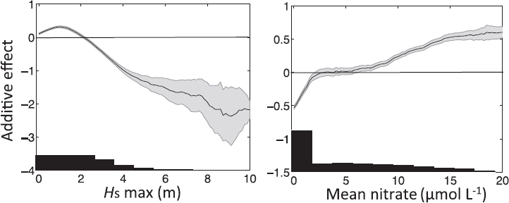
imagery from the California coast are used to assess the controls on their population density (Bell et al., 2015a). Giant kelp populations are controlled by many processes, including nitrate availability and disturbance from surface waves forcings. Figure 8.6 shows the additive effects for changes in significant wave height (left) and nitrate concentrations (right). This demonstrates detrimental threshold effects on California giant kelp forests for significant wave heights above 3 meters and nitrate concentration below 2 µM. Positive effects are also found for smaller significant wave heights (HS ≤ 2 m) and nitrate concentrations above 7 µM. Similar threshold detection analyses can be conducted for other ecosystems.
Better estimation of carbon emissions of terrestrial ecosystems from disturbance, particularly fire severity related to thresholds of warming and drying, have the potential to dramatically increase our ability to model combustion of forest biomass as well as soil organic matter, particularly in high-latitude ecosystems. Threshold changes in terrestrial ecosystems are particularly relevant to rapid thawing and degradation of permafrost carbon as the freezing temperature threshold of melting ice is crossed at greater depths (Schuur et al., 2015; Schädel et al., 2016). This issue is exacerbated when fire disturbance combusts insulating soil layers and accelerates the rate of permafrost thaw (Grosse et al., 2011). These issues are addressed in greater detail in a recent National Academy workshop report (NRC, 2014).
Measurement Approaches
The measurement approach for elucidating ecological threshold and cascading effects on carbon storage will require the satellite observation of the stocks and fluxes for the ecosystem of interest as well as indices for processes known to affect the ecosystem. For the kelp forest ecological thresholding example earlier (see Figure 8.6), kelp biomass variations in time and space from Landsat imagery are compared with significant wave height and nitrate concentration estimates based on remote sensing, field observations, and models (see Bell et al., 2015a, for details). In this example, generalized additive models (GAMs; Hastie and Tibshirani, 1990; Wood, 2006) were used to quantify the nonlinear responses of the population density (kelp canopy biomass) to known forcing time series (see Figure 8.6). Many other statistical techniques can be used to assess ecological thresholds. The extension of this approach to other ecosystems is clearly dependent upon the ecosystem to be explored and known processes driving its variability in its components. Key for the elucidation of ecological thresholds from remote sensing observations are extensive data on ecosystem stocks and potentially rates and concurrent forcings on the appropriate time and space scales. The previous sections of this report provided approaches for assessing ecosystem stocks and rates that would useful for this general approach for quantifying ecological thresholds from satellite observations.
Objective E-5b
Objective E-5b. Discover cascading perturbations in ecosystems related to carbon storage.
Motivation
The panel identified discovering cascading perturbations in ecosystems related to carbon storage as an Important priority.
Alterations or perturbations in one component of an ecosystem may have cascading impacts for the entire ecosystem via altering rates of disturbance, trophic interactions, or other ecological processes. Improved understanding of the extent and direction of these relationships is critical for understanding ecosystem changes in a changing climate. This panel focused on the role of cascading perturbations in
ecosystems in the context of altering C storage. Three examples of perturbations that can significantly affect carbon storage are wildfire, permafrost thaw, and pine beetle infestations.
Permafrost Thaw, Fire Regimes, and Their Interactions
Fire plays an integral role in shaping the surface properties of ecosystems underlain by permafrost, and a recent shift to larger and more severe fires (Mack et al., 2011; Turetsky et al., 2011) already indicates a shift toward a more intense fire regime in boreal (Kelly et al., 2013) and even in tundra areas (Higuera et al., 2011). The severity of burning modifies soil organic layer depth, with cascading effects on surface energy balance, active layer thickness, surface hydrology, and vegetation succession (Boby et al., 2010; Grosse et al., 2011). The implications of this shift in the fire regime on permafrost thaw are important for quantifying potentially large positive feedbacks to climate warming, but are currently poorly understood or quantified over spatial extents larger than field plots.
A large and growing body of evidence documents how permafrost thaw, and the consequent mobilization of its long-sequestered carbon to the atmosphere, can greatly amplify warming via a positive feedback cycle of albedo changes and thawing (Schuur et al., 2007; Schädel et al., 2016).
Forest diebacks impact climate through decreased evapotranspiration. Maness et al. (2013) showed that pine beetle infestation of British Columbia in an area of 170,000 km2 led to a warming of 1°C.
As discussed in Objective E-3a, wildfires are also a key influence on other ecosystems and the carbon cycle.
Pine Beetle Infestation
Infestations by pine beetles and other pests lead to large-scale forest diebacks, with subsequent reduction of photosynthesis and enhancement of decomposition. Assessing the impact of insect infestations on carbon storage require inventories of forest biomass and function before and after the dieback.
Measurement Objectives and Approaches for Three Key Ecosystem Perturbations
As discussed earlier, wildfires, permafrost thaw, and pine beetle infestations represent only three examples of cascading perturbations in ecosystems. The measurements and approaches necessary to examine other cascading perturbations may vary. In the following, the panel discusses those that would address our three examples.
Satellite observations of biomass burning involve using MODIS and VIIRS 3.5-4.0 µm data to map the combustion temperature and location of active or smoldering fires. Measurements of vegetation forest structure can be retrieved from spaceborne lidar similar to the GEDI and ICESat-2 missions. Sustained land imaging from Landsat-8, Sentinel-2a, and Sentinel-2b provide 30 m spatial mapping of forests that, when combined with forest vertical structure, enables forest biomass to be determined from space. Identification of community composition and comparisons between the prefire forest composition and density and the postfire observations provides the type and degree of how much the vegetation in question was consumed in the fire.
Sustained measurements are needed to document the influence and implications of fire disturbance on permafrost thaw. Fire disturbance extent, timing, and severity can be readily mapped using optical imagery, but changes in permafrost properties require measurements of surface deformation from repeat lidar and interferometric SAR (e.g., Short et al., 2011; Chen et al., 2012). Sustained measurements are also needed to establish meaningful baselines against which future change can be assessed (Grosse et al., 2016; Jorgenson and Grosse, 2016).
Achieving an inventory of forest biomass and function before and after a pine beetle or other insect infestation can be accomplished by observations of leaf chlorophyll via Normalized Difference Vegetation Index (NDVI), GPP via SIF, and aboveground biomass via lidar.
Objective E-5c
Objective E-5c. Understand ecosystem response to fire events.
Motivation
The panel identified improved understanding of ecosystem response to fire events as an Important priority.
Smoke emissions from wildfires are injected into the atmosphere, acting as air pollutants including gases and aerosols and affecting atmospheric thermodynamics, altering local-to-regional weather and larger-scale climate systems. Fire emissions affect climate systems by producing cloud condensation nuclei (Hobbs et al., 1997) and aerosols that directly and indirectly affect radiative forcing and altering the radiation balance of the land surface (vegetation change, deposition on ice; Randerson et al., 2006). Aerosols can influence the cloud formation, thereby impacting the energy balance and the hydrological cycle. Smoke can also contain limiting nutrients, affecting both land and ocean ecosystems (Schulz et al., 2012).
Fire influences ecosystem health by affecting the biogeochemistry of carbon and nitrogen cycles and thereby affecting nutrient availability and ecosystem productivity. The ability to map and monitor postfire recovery provides important information for proper natural resource management and allows resource managers to make decisions affecting biodiversity, species protection, and overall ecosystem health.
Fire affects atmospheric thermodynamics by impacting flows of carbon and energy in terrestrial, atmospheric, and hydrologic subsystems of the biosphere and thereby influences the global climate system. Specifically, fires contribute to increasing atmospheric carbon, which impacts the climate system. But importantly, fires also substantially impact nutrient cycling and affect carbon uptake by the biosphere and impose constraints on how the carbon cycle responds to variations in climate (Thornton et al., 2007). The incomplete combustion of biomass produces varying forcing agents, including changed surface albedo from black carbon, which can absorb and scatter solar radiation, deposit on snow and ice to change surface albedo, and effects on cloud properties and formulation (Randerson et al., 2006).
As described in Objective E-2c, black carbon is a short-term atmospheric pollutant that results from incomplete combustion of carbonaceous fuels from industrial sources and from open biomass burning. Recent estimates (Bond et al., 2013) have placed black carbon as the second most important anthropogenic climate forcing (+1.1 W/m2) relative to carbon dioxide forcing (1.83 W/m2). However, the influence of black carbon on the climate is complex, as it has a direct effect on atmospheric warming due to absorption of shortwave radiation and an indirect influence such as change in surface albedo of snow and ice in polar regions (AMAP, 2011).
Measurement Objectives
Sustained satellite observations of fire activity including characterizations of fire occurrence, fire area, fire temperature, and fire radiative power (FRP) are required to assess global impacts of wildfires.
Forest Recovery
Vegetation composition can be characterized by vegetation functional types as measured by assemblages of species by structure, physiology, and phenology that characterize ecosystem response to environmental conditions or disturbance severity. New technologies provide continuous characterization of optical classes that inform functional type classifications and map functional diversity, which can be linked to biodiversity within ecosystems. Vegetation structure requires observations of mean and variation of canopy height, canopy base height, stem density, stem volume, basal area, and fractional canopy cover.
Canopy Carbon and Nitrogen Composition
Mapping canopy chemical composition characterizes the vegetation. Additionally, mapping canopy fuel load using aboveground biomass and leaf area index is essential for refining estimates of fire carbon fluxes and pre- and postfire carbon and nitrogen stocks.
Ecosystem condition can be characterized by the following:
- Discrimination between live, senescent/scorched, and charred vegetation, which can inform the health of the ecosystem and provide information on burn fraction.
- Measurement of vegetation stress, which is a critical observation for understanding how flammable an ecosystem is, including observations of precipitation, temperature, relative humidity, wind speed and direction, soil moisture, soil temperature, and vegetation water content or equivalent water thickness.
- Measurement of ecosystem flux affecting fuel accumulation and mapping postfire regeneration. For this, observations are needed of gross primary productivity, which can be derived from fraction of photosynthetic active radiation, leaf area index, vegetation photosynthetic capacity, and solar-induced fluorescence.
Measurement Approaches
Reliable detection of wild and prescribed fires and associated fuel loads requires measurements across three platforms: (1) thermal infrared radiometer (TIR); (2) a visible-shortwave-infrared imaging spectrometer; and (3) an active sensor to detect 3D vegetation structure.
Fire detections and land surface temperature need sustained global TIR radiometric retrievals at ≤375 m pixel resolution at nadir ± 60 degrees, with subdaily observations with at least nine bands at ~8.3 µm, ~8.6 µm, ~9.1 µm, ~11 µm, ~12 µm to distinguish land surface temperature from emissivity, ~4 µm with ≥400 K saturation and sufficient thermal range for fire detections, and two bands (~1.6 µm and ~2.2 µm) to have sufficient sensitivity at the lower temperatures for cloud detection, geolocation, and flagging false positives (Schroeder et al., 2014).
Vegetation functional types, gross primary productivity, and fire severity need continued coverage through recovery from imaging spectrometer data. A VSWIR imaging spectrometer is needed with continuous spectral range 0.4-2.5 µm at ≤10 nm spectral sampling, ≤30 m pixel resolution, ≤16-day observation repeat, a 185 km swath, and high signal-to-noise and global coverage. This provides Landsat spatial resolution hyperspectral observations using spectral-response functions; canopy chemical composition and equivalent water thickness; and live, senescent or scorched, and charred vegetation characterization.
Vegetative structure and aboveground biomass can be observed using full waveform or discrete return lidar and single-band microwave synthetic aperture radar (SAR; Lefsky et al., 2002; Neuenschwander et al., 2006). Use of full waveform lidar can improve penetration of dense vegetation structure for improved characterization. Lidar can also be used to obtain vertical profiles of atmospheric plumes containing black
carbon (e.g., the CALIPSO satellite). SAR has the advantage of penetrating cloud cover and providing measurement of soil moisture and vegetation water content, which are important factors in fire intensity.
Consistent TIR measurements are required across missions or through continued existence of these missions. It is assumed that measurements from MODIS and VIIRS will continue through the National Polar-Orbiting Operational Environmental Satellite System (NPOESS) and JPSS programs. To advance beyond current status requires a new global mapping mission that ideally increases the saturation temperature while providing subdaily <375 m pixel resolution. Requirements for a VSWIR imaging spectrometer have a strong legacy of previous investments in response to the 2007 NRC Decadal Survey (NRC, 2007) and the 2014 NRC sustainable land imaging report (NRC, 2014).
Many existing satellites have proven the feasibility and affordability for collecting measurements characterizing Earth’s surface from active sensors (both lidar and SAR). But more research is needed for development of better algorithms that extract needed information and bridge observations across satellite platforms.
To characterize black carbon emissions and track transport to remote locations, a vertical lidar is needed similar in concept to the CALIOP instrument. CALIOP successfully demonstrated the utility and feasibility of these measurements from space.
Connections to Other Panels
This objective has many connections to several other panels. It especially relates to extreme events affecting water, weather, and the solid Earth (e.g., Questions C-7, C-8, H-4, W-4, S-1, and S-2).
Connections to the Hydrology Panel include their objective to quantify the magnitude of anthropogenic causes (e.g., forest management, black carbon, and infrastructure) that affect snowmelt and icemelt (Questions H-1 and H-4). Question E-5 also relates to the Hydrology Panel’s objectives to understand linkages between anthropogenic modification of the land, including fire suppression, land use, and urbanization on frequency of and response to hazards (Questions H-2 and H-4).
Connections to other panels include synergies with the Climate Panel’s objectives for quantifying variations in the global carbon cycle and associated climate and ecosystem impacts in the context of past and projected anthropogenic carbon emissions, and assessing uncertainty in total climate forcing that arises from aerosol changes and their interactions with clouds (Questions C-2, C-3, and C-5). An example is the Climate Panel’s Question C-5, which asks how changes in aerosols affect Earth’s radiation budget and how to better quantify the magnitude and variability of emissions of natural aerosols. Connections to the Hydrology Panel include their objective (H-2b) to quantify the magnitude of anthropogenic activities (e.g., forest management, black carbon, and infrastructure) that affect snowmelt and icemelt, atmospheric radiation, and temperature changes, thereby altering downstream distribution of water quantity and quality. Another connection to the Hydrology Panel is their Objective H-4d, which seeks to understand linkages between anthropogenic modification of the land, including fire suppression, land use, and urbanization on frequency of and response to hazards.
RESULTING SOCIETAL BENEFIT
The resulting societal benefits of achieving the stated objectives cover a broad range of both direct and indirect benefits. The direct benefits include more precise and comparable measurements of the structure, composition, and dynamics of terrestrial and marine biomass (Objectives E-1a, E-1b, and E-1c) as well as the fluxes and flows of carbon and energy between ecosystems and the atmosphere (Objectives E-2a and E-3a). These direct observations provide evidence-based decision support to inform a wide array of eco-
nomically important applications concerning the sustainable management of terrestrial landscapes, coastal environments, and open-ocean ecosystems. For example, these observations provide the detailed time series required to monitor the health and productivity of both managed and natural vegetated landscapes as well as highly dynamic coastal and ocean biological processes. Specific data products will inform a wide range of critical resource management sectors including forestry, agriculture, water management, public health, fisheries, disaster relief, and conservation management.
For example, the same satellite observations identified for measuring land GPP have direct use in accurately estimating global agricultural production and are used to provide monthly reports that remove uncertainty in global agricultural markets (USDA, 2017) and provide the satellite data used by GEO GLAM. The same satellite observations that enable land GPP measurements are also used to predict extensive outbreaks of mosquito-borne diseases of dengue, Rift Valley fever, Murray Valley encephalitis, and West Nile virus (Anyamba et al., 2014). Landsat data that have been widely used to document forest disturbance and recovery at the 30 m scale globally for carbon cycle research have also been used to manage forest resources for countries at the national level (Hansen et al., 2013). In addition to direct resource management, data products and information derived from these objectives will inform critical national and international efforts to better manage GHG emissions and carbon sequestration.
Earth observations data products and synthesis information derived from meeting the stated objectives will also support a number of national and international agreements and objectives. These include international agreements on sustainable use of the oceans, trade in endangered species, economic and trade agreements related to timber and agriculture, reducing emissions from deforestation and forest degradation, and the UN Sustainable Development Goals. Observations here will also support national laws and polices such as the Soil and Water Conservation Act (SWCA), the National Environmental Policy Act (NEPA), the Clean Water Act (CWA), the Safe Resource Conservation and Recovery Act (RCRA), the Comprehensive Environmental Response, Compensation, and Liability Act/Superfund Amendments and Reauthorization Act (CERCLA/SARA), the Endangered Species Act (ESA), the Marine Mammal Protection Act (MMPA), the Magnuson-Stevens Fishery Conservation and Management Act, and a variety of other standing societal mandates.
Here, the panel provides some specific examples of societal benefits from land and ocean ecosystem observations.
United Nations Sustainable Development Goals
These observations support at least three important international sustainable development goals. First, United Nations Sustainable Development Goal (SDG) 14 focuses on conservation and sustainable use of the oceans, seas, and marine resources, specifically economic utilization of natural resources of marine systems using evidence-based and data-rich management approaches. Second, SDG 15.2 focuses on sustainable management of forests, including reducing deforestation and increasing afforestation and reforestation throughout the world. Third, SDG 15.3 seeks to combat desertification and reverse land degradation. The ocean and terrestrial ecosystem characterization and monitoring objectives (Objectives E-1a, E-1b, E-1c, E-1e, E-3a, and E-5c) of this effort will specifically inform these stated international development goals.
Emerging International Coordination Mechanisms for Earth Observations
As Earth observing systems proliferate internationally, and many new countries begin to contribute their space assets and observations to a growing global pool of measurements, the international community is
responding through increased coordination of programs, with a high priority on societal benefits of the combined observing systems. The ecosystem observations defined here are critical contributions.
The Group on Earth Observing Biodiversity Observing Networks (GEO-BON) in collaboration with other initiatives are prioritizing the development of Essential Biodiversity Variables (EBVs) to provide measurement and monitoring of ecological condition and ecosystem services to inform international agreements and protocols, such as the Convention on Biological Diversity (CBD), the Convention on Migratory Species (CMS), and the Intergovernmental Science-Policy Platform on Biodiversity and Ecosystem Services (IPBES). The CBD uses remote sensing products to evaluate the distribution and status of habitats, and the CMS uses remote sensing data to evaluate the connectivity of habitats and populations for migratory species. Both of these conventions interact directly with the United Nations Environment Program (UNEP) on endangered wildlife species as well as the International Union for Conservation of Nature (IUCN) “red list” listing of endangered species and illegal wildlife trade.
Similarly, the Global Ocean Observing System (GOOS) has developed complementary Essential Ocean Variables (EOVs) for Biology and Ecosystems that include phytoplankton biomass and diversity, live coral, macroalgal canopy, and seagrass cover, all of which specify remote sensing as a critical tool, while the GOOS Biogeochemistry Panel has defined an Ocean Color EOV. This panel’s stated objectives closely support these established initiatives. The Global Observations of Forest Initiative is an international attempt to coordinate observing systems and measurements for forest status, health, and carbon stocks. The GEO GLAM initiative is addressing global land and agriculture monitoring systems. The ecosystem measurements found in all of the science objectives here will provide significant contributions from NASA and the United States to the international collection of observations. The ocean and terrestrial ecosystem characterization and monitoring objectives (Objectives E-1a, E-1b, E-1c, and E-1e) of this effort will specifically inform these stated international development goals.
National Forest Monitoring Systems for Sustainable Forest Management and GHG Inventory
For many developing countries, conversion and degradation of forests is the most significant source of greenhouse gases (GHGs), often in far greater amounts than from industrial sources. International estimates of GHG emissions from many developing countries reflect a clear picture of socioeconomic circumstances: economies dependent on agriculture and natural resources, with small and underdeveloped energy and industrial sectors. Recent reports document large current emissions as well as project large future emissions from forest conversion and degradation. Taking action to reduce these emissions is a fundamental aim of international climate change mitigation programs.
This international mitigation initiative, commonly termed REDD+ (reduce emissions from deforestation and forest degradation), is a policy process that incentivizes reductions in emissions from forested lands and encourages investments in low-carbon, sustainable development, particularly in developing countries. It does so by assigning financial value to carbon stored in forests. REDD+ goes beyond deforestation and forest degradation, and includes the role of conservation, sustainable management of forests, and enhancement of forest carbon stocks. Outside the diplomatic policy process associated with the conventions, other multilateral REDD+ initiatives are being implemented to provide private capital and large financial investments in low-carbon forest management. These initiatives include the Forest Carbon Partnership Facility (FCPF), hosted by the World Bank, and the Forest Investment Program (FIP), implemented by various multilateral development banks, including the African Development Bank. There are different types of potential arrangements for achieving REDD+ results: private-private, public-private, nongovernmental organization (NGO)-public, as programs with subnational jurisdictions, or as federal government policy.
Each of these domains has significant technical requirements for measurement and monitoring of forests that would immediately benefit from Objectives E-1a, E-1b, E-1e, and E-3a. The international conventions advise countries that are implementing REDD+ activities to follow specific methodologies for estimating GHG emissions and removals developed by the International Panel on Climate Change (IPCC). These methodologies require a system for estimating forest GHG stocks and fluxes, using a national forest monitoring and measurement system (NFMS). Thus, all countries participating in REDD+ actions and programs need to have a basic level of “readiness” for implementing a NFMS to produce the data needed for REDD+ measurement, reporting, and verification (MRV) focused on carbon accounting.
In most countries with deforestation-related GHG emissions, and where forestland is an important national resource, increasing technical capacity to monitor and measure forest status and condition through a NFMS will have both climate and economic benefits. The services that forest and woodlands provide to these countries are numerous—including food, water, and fuel. However, these ecosystems are decreasing at rapidly increasing rates owing to unsustainable use of fuel wood and charcoal, poor agricultural practices, limited economic choices, and high population growth. Earth Observations will contribute to building capacities for REDD+ MRV. REDD+ offers a holistic framework for supporting sustainable land management by integrating policy and resource governance in the rural landscape with the development of analytical capacities and economic incentives.
Sustainable forest management and GHG emission reductions actions require countries to develop national platforms for measuring, reporting, and verifying GHG emissions and removals on a regular basis. For the most part, this requires that countries have the technical capacity to systematically measure a set of factors related to (1) changes in the extent and condition of forest cover; (2) carbon stocks in forests of various stature and condition, and changes over time in those stocks; and (3) emissions or removals of GHGs associated with changes in forest cover and changes in carbon stocks.
Precision Agriculture
Satellite data such as Landsat 30 m and comparable foreign satellite imagery have been used to evaluate agricultural fields impacted by weeds, excessive moisture, low soil pH, or an imbalance of plant nutrients (Johannsen and Daughtry, 2009; see Figure 8.7). Recently, commercial multispectral imagery from Ikonos, World View, GeoEye, QuickBird, and other satellites at a 1 m to 4 m spatial resolution has been available to farmers for the management of high-value crops such as vineyards, fruit orchards, and vegetables, although the cost of obtaining these data has been prohibitive for widespread use.
The recent development and use of small imagers on Unmanned Aerial Vehicles and on tractors, both linked to global positioning systems, provides an alternative platform with greater flexibility for digital image data collection with improved spatial resolution, very frequent data collection, and a significantly lower cost. The within-field collection of remotely sensed multispectral imagery has enabled what is now known as “precision agriculture.” These precision technologies developed for agriculture include accurate identification of within-field fertilizer application rates, “smart irrigation systems” that work along with remotely sensed images to maximize water use efficiency based on plant needs, evaporation rates, soil texture, and soil structure. These systems minimize irrigation frequency and avoid unnecessary fertilizer application expenses while increasing yield and improving crop product quality.
While commercial remote sensing companies have provided these services in the past to farmers, precision farming now permits farmers to perform more timely operations related to better soil management such as tillage, plan more accurate crop-protection programs, adjust seeding rates, and map the yield variability commonly caused by soil and nutrient differences within fields. Farmers can now implement variable-rate nutrient fertility plans, including applying nitrogen when planting crops and applying nitro-
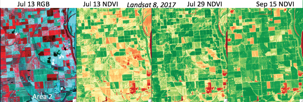
gen during cultivation only when needed. This translates into a greater net return per acre and improved management of seeding rates, specific application of fertilizers, and specific applications of agricultural chemicals. This also leads to improving soils, reducing the loss of topsoil, and minimizing water quality threats. This potential depends on the farmer’s management skill and frequently on the services of a knowledgeable crop consultant. Precision agriculture’s use of multispectral remote sensing coupled with accurate GPS location information involves the 4Rs—right product, right rate, right time, and right place (Johannsen et al., 1997).
Another benefit of precision agriculture is that remotely sensed data can be analyzed and geocoded and merged with soil maps, to establish a digital record of field operation by year. This can be used to guide further field operations in future years and establishes a permanent farm record. For example, this means that remotely sensed data would complement the yield data collected by the farmer’s harvesting equipment and identify specific locations of yield variations within a crop field for diagnostic postharvest analysis (Johannsen and Carter, 2002).
Commercial remote sensing companies have also used weekly images to map the acreage of agricultural crops and monitor their conditions throughout the growing season. The images and interpretations provide farmers with a better bargaining position when selling their crops, since they have knowledge of their crops’ progress as well as how their competitor’s crops are doing.
In addition to the tractor-mounted imagers and imagers on UAVs, Planet, a commercial company, is moving forward with daily 5 m global visible and near-infrared data (Planet Team, 2017). This is a good example of work begun by the U.S. government with the Landsat series of satellites, where applications of satellite technology led to demonstrating the potential of remote sensing in agriculture. Developments in smaller satellites like Planet’s CubeSats, the development of UAVs with imagers, and the development of imagers on tractor, all linked to GPS systems, will advance precision agriculture while sustaining our agricultural lands.
Over 60 percent of the farmers in the United States are now using forms of precision agriculture. New observations proposed in this chapter—specifically, hyperspectral and multitemporal multispectral—could begin layering plant physiological and process-level information on agricultural maps as well (Johannsen and Carter, 2004).
Ocean and Marine Health Monitoring
There are many societal benefits of ocean color remote sensing that are fairly well established, having been developed and expanded upon over three decades of practice. Increasing economic costs are associated with unhealthy marine systems, and improvements in management depend on improved monitoring. Advancements in technologies and science applications (Objectives E-1b and E-1c) should enhance the benefits that already exist, as well as lead to novel ones, as in the following examples:
- Creation of cost-effective ecological indicators, which can be applied to ecosystem-based management and characterization of change due to natural and anthropogenic perturbations or disturbances;
- Monitoring of the onset, expansion, and fate of harmful algal blooms, aiding the tourism and aquaculture industries;
- Monitoring of coastal water quality as a tool in coastal zone management;
- Delineation of marine protected areas and identification of habitats for threatened/endangered species;
- Sustainable management of fisheries and more cost effective harvesting;
- Measurement of phytoplankton photosynthesis, which is essential information for ocean ecosystem models, as well as for understanding the role of the ocean in climate change and global carbon cycles;
- Creation of outstanding material for education at all levels, both in formal classroom environments and in informal education, developing public awareness of ocean processes; and
- International governance on the high seas.
The coastal zone, especially shallow waters <30 m depth, represent a very small proportion of the global ocean area, yet coastal ecosystems are among the most productive in the world. Importantly, about 40 percent of the world’s human population lives within 100 km of the coast (United Nations, 2007). The social and economic well-being of people living in these regions is inextricably linked with the surrounding coastal ecosystem. Information about this ecosystem provided by high spatial and high spectral resolution remote sensing (Objective E1-a) stands to be of great societal benefit, as follows:
- Creation of new baseline global maps of wetland distribution, type, and composition, leading to better understanding of change in wetlands ecosystem goods and services;
- Creation of critical ecology and resource inventories for coral reefs, seagrasses, kelp, and other submerged aquatic systems;
- Identification and delineation of coastal fisheries habitats, with applications to management and enforcement;
- Measuring and monitoring of changes in biodiversity;
- Improved coastline mapping and tracking of shoreline changes; and
- Creation of outstanding material for education at all levels, both in formal classroom environments and in informal education, developing public awareness of ocean processes.
REFERENCES
Abatzoglou, J.T., and A.P. Williams. 2016. Impact of anthropogenic climate change on wildfire across western US forests. Proceedings of the National Academy of Sciences 113:11770-11775.
Anav, A., P. Friedlingstein, C. Beer, P. Ciais, A. Harper, C. Jones, G. Murray-Tortarolo, D. Papale, N.C. Parazoo, and P. Peylin. 2015. Spatiotemporal patterns of terrestrial gross primary production: A review. Reviews of Geophysics 53:785-818.
Anderegg, W.R.L., J.A. Hicke, R.A. Fisher, C.D. Allen, J. Aukema, B. Bentz, S. Hood, et al. 2015. Tree mortality from drought, insects, and their interactions in a changing climate. New Phytologist 208:674-683.
Anderson, M.C., W.P. Kustas, J.M. Norman, C.R. Hain, J.R. Mecikalski, L. Schultz, M.P. González-Dugo, C. Cammalleri, G. D’urso, A. Pimstein, and F. Gao. 2011. Mapping daily evapotranspiration at field to continental scales using geostationary and polar orbiting satellite imagery. Hydrology and Earth System Sciences 15:223-239.
Anderson, M.C., R.G. Allen, A. Morse, and W.P. Kustas. 2012. Use of Landsat thermal imagery in monitoring evapotranspiration and managing water resources. Remote Sensing of Environment 122:50-65.
Anyamba, A., J.L. Small, S.C. Britch, C.J. Tucker, E.W. Pak, C.A. Reynolds, J. Crutchfield, and K.J. Linthicum. 2014. Recent weather extremes and impacts on agricultural production and vector-borne disease outbreak patterns. PLoS One 9:e92538.
AMAP (Arctic Monitoring and Assessment Programme). 2011. The Impact of Black Carbon on Arctic Climate (2011). Oslo, Norway.
Arneth, A., S. Sitch, J. Pongratz, B. Stocker, P. Ciais, B. Poulter, A. Bayer, A. Bondeau, L. Calle, and L. Chini. 2017. Historical carbon dioxide emissions caused by land-use changes are possibly larger than assumed. Nature Geoscience 10:79-84.
Arnone, R., R. Vandermeulen, S. Ladner, M. Ondrusek, C. Kovach, H. Yang, and J. Salisbury, 2016. Diurnal changes in ocean color in coastal waters. Ocean Sensing and Monitoring VIII 9827:982711.
Arora, V.K., G.J. Boer, P. Friedlingstein, M. Eby, C.D. Jones, J.R. Christian, G. Bonan, L. Bopp, V. Brovkin, and P. Cadule. 2013. Carbon-concentration and carbon-climate feedbacks in CMIP5 Earth system models. Journal of Climate 26:5289-5314.
Asner, G.P., D.E. Knapp, C.B. Anderson, R.E. Martin, and N. Vaughn. 2016a. Large-scale climatic and geophysical controls on the leaf economics spectrum. Proceedings of the National Academy of Sciences 113:E4043-E4051.
Asner, G.P., D.E. Knapp, T. Kennedy-Bowdoin, M.O. Jones, R.E. Martin, J. Boardman, and R.F. Hughes. 2008. Invasive species detection in Hawaiian rainforests using airborne imaging spectroscopy and LiDAR. Remote Sensing of Environment 112:1942-1955.
Asner, G.P., P.G. Brodrick, C.B. Anderson, N. Vaughn, D.E. Knapp, and R.E. Martin. 2016b. Progressive forest canopy water loss during the 2012-2015 California drought. Proceedings of the National Academy of Sciences 113:E249-E255.
Asner, G.P., and R.E. Martin. 2016. Spectranomics: Emerging science and conservation opportunities at the interface of biodiversity and remote sensing. Global Ecology and Conservation 8:212-219.
Asner, G.P., R.E. Martin, D.E. Knapp, R. Tupayachi, C.B. Anderson, F. Sinca, N.R. Vaughn, and W. Llactayo. 2017. Airborne laser-guided imaging spectroscopy to map forest trait diversity and guide conservation. Science 355:385-389.
Asner, G.P., R.E. Martin, R. Tupayachi, R. Emerson, P. Martinez, F. Sinca, G.V.N. Powell, S.J. Wright, and A.E. Lugo. 2011. Taxonomy and remote sensing of leaf mass per area (LMA) in humid tropical forests. Ecological Applications 21:85-98.
Asner, G.P., R.E. Martin, R. Tupayachi, C.B. Anderson, F. Sinca, L. Carranza-Jiménez, and P. Martinez. 2014. Amazonian functional diversity from forest canopy chemical assembly. Proceedings of the National Academy of Sciences 111:5604-5609.
Atzberger, C. 2013. Advances in remote sensing of agriculture: Context description, existing operational monitoring systems and major information needs. Remote Sensing 5:949-981.
Baccini, A., S.J. Goetz, W.S. Walker, N.T. Laporte, M. Sun, D. Sulla-Menashe, J. Hackler, P.S.A. Beck, R. Dubayah, M.A. Friedl, S. Samanta, and R.A. Houghton. 2012. Estimated carbon dioxide emissions from tropical deforestation improved by carbon-density maps. Nature Climate Change 2:182-185.
Badgley, G., C.B. Field, and J.A. Berry. 2017. Canopy near-infrared reflectance and terrestrial photosynthesis. Science Advances 3:e1602244.
Baldeck, C.A., G.P. Asner, R.E. Martin, C.B. Anderson, D.E. Knapp, J.R. Kellner, and S.J. Wright. 2015. Operational tree species mapping in a diverse tropical forest with airborne imaging spectroscopy. PLoS One 10:e0118403.
Ballantyne, A., W. Smith, W. Anderegg, P. Kauppi, J. Sarmiento, P. Tans, E. Shevliakova, Y. Pan, B. Poulter, and A. Anav. 2017. Accelerating net terrestrial carbon uptake during the warming hiatus due to reduced respiration. Nature Climate Change 7:148-152.
Barthlott, W., W. Lauer, and A. Placke. 1996. Global distribution of species diversity in vascular plants: Towards a world map of phytodiversity (Globale Verteilung der Artenvielfalt Höherer Pflanzen: Vorarbeiten zu einer Weltkarte der Phytodiversität). Erdkunde 50:317-327.
Bastos, A., S.W. Running, C. Gouveia, and R.M. Trigo. 2013. The global NPP dependence on ENSO: La Nina and the extraordinary year of 2011. Journal Geophysical Research: Biogeosciences 118:1247-1255.
Basu, S., S. Guerlet, A. Butz, S. Houweling, O. Hasekamp, I. Aben, P. Krummel, P. Steele, R. Langenfelds, and M. Torn. 2013. Global CO2 fluxes estimated from GOSAT retrievals of total column CO2. Atmospheric Chemistry and Physics 13:8695-8717.
Beer, C., M. Reichstein, E. Tomelleri, P. Ciais, M. Jung, N. Carvalhais, C. Rödenbeck, M.A. Arain, D. Baldocchi, and G.B. Bonan. 2010. Terrestrial gross carbon dioxide uptake: Global distribution and covariation with climate. Science 329:834-838.
Behrenfeld, M.J., and P.G. Falkowski. 1997. Photosynthetic rates derived from satellite-based chlorophyll concentration. Limnology and Oceanography 42:1-20.
Behrenfeld, M.J., E. Boss, D.A. Siegel, and D.M. Shea. 2005. Carbon based ocean productivity and phytoplankton physiology from space. Global Biogeochemical Cycles 19.
Behrenfeld, M.J., R.T. O’Malley, D.A. Siegel, C.R. Mcclain, J.L. Sarmiento, G.C. Feldman, A.J. Milligan, P.G. Falkowski, R.M. Letelier, and E.S. Boss. 2006. Climate-driven trends in contemporary ocean productivity. Nature 444:752-755.
Behrenfeld, M.J., T.K. Westberry, E.S. Boss, R.T. O’Malley, D.A. Siegel, J.D. Wiggert, B. Franz, C. McClain, G. Feldman, and S.C. Doney. 2009. Satellite-detected fluorescence reveals global physiology of ocean phytoplankton. Biogeosciences 6:779-794.
Behrenfeld, M.J., S.C. Doney, I. Lima, E.S. Boss, and D.A. Siegel. 2013. Annual cycles of ecological disturbance and recovery underlying the subarctic Atlantic spring plankton bloom. Global Biogeochemical Cycles 27:526-540.
Behrenfeld, M.J., Y. Hu, C.A. Hostetler, G. Dall’Olmo, S.D. Rodier, J.W. Hair, and C.R. Trepte. 2013. Space based lidar measurements of global ocean carbon stocks. Geophysical Research Letters 40:4355-4360.
Behrenfeld, M.J., Y. Hu, R.T. O’Malley, E.S. Boss, C.A. Hostetler, D.A. Siegel, J.L. Sarmiento, J. Schulien, J.W. Hair, X. Lu, S. Rodier and A.J. Scarino. 2017. Annual boom-bust cycles of polar phytoplankton biomass revealed by space-based lidar. Nature Geoscience 10:118-122.
Bell, T.W., K.C. Cavanaugh, D.C. Reed, and D.A. Siegel. 2015a. Geographical variability in the controls of giant kelp biomass dynamics. Journal of Biogeography 42:2010-2021.
Bell, T.W., K.C. Cavanaugh, and D.A. Siegel, 2015b. Remote monitoring of giant kelp biomass and physiological condition: An evaluation of the potential for the Hyperspectral Infrared Imager (HyspIRI) mission. Remote Sensing of the Environment 167:218-228.
Ben-Dor, E., S. Chabrillat, J.A.M. Demattê, G.R. Taylor, J. Hill, M.L. Whiting, and S. Sommer. 2008. Using imaging spectroscopy to study soil properties. Remote Sensing of Environment 113:S38-S55.
Ben-Dor, E. and J. Demattê. 2016. Remote Sensing of Soil in the Optical Domains. In Land Resources Monitoring, Modeling, and Mapping with Remote Sensing (Prasad S. Thenkabail, ed.). Boca Raton, FL: CRC Press.
Bergen, K., S. Buckley, C. Dobson, A. Donnellan, R. Dubayah, Y. Fialko, E. Fielding, et al. (DESDynI Writing Committee). 2007. Report of the July 17-19, Orlando, Florida Workshop to Assess the National Research Council Decadal Survey Recommendation for the DESDynI Radar/Lidar Space Mission. https://cce.nasa.gov/pdfs/Volz2_DESDynI.pdf.
Bergen, K.M., S.J. Goetz, R.O. Dubayah, G.M. Henebry, C.T. Hunsaker, M.L. Imhoff, R.F. Nelson, G.G. Parker, and V.C. Radeloff. 2009. Remote sensing of vegetation 3-D structure for biodiversity and habitat: Review and implications for lidar and radar spaceborne missions. Journal of Geophysical Research: Biogeosciences 114.
Boby, L.A., E.A.G. Schuur, M.C. Mack, D. Verbyla, and J.F. Johnstone. 2010. Quantifying fire severity, carbon, and nitrogen emissions in Alaska’s boreal forest. Ecological Applications 20:1633-1647.
Bolten, J.D., and W.T. Crow. 2012. Improved prediction of quasi-global vegetation conditions using remotely-sensed surface soil moisture. Geophysical Research Letters 39.
Bond, T.C., S.J. Doherty, D. Fahey, P. Forster, T. Berntsen, B. Deangelo, M. Flanner, S. Ghan, B. Kärcher, and D. Koch. 2013. Bounding the role of black carbon in the climate system: A scientific assessment. Journal of Geophysical Research: Atmospheres 118:5380-5552.
Bond-Lamberty, B., and A. Thomson. 2010. Temperature-associated increases in the global soil respiration record. Nature 464:579.
Bopp, L., C. Le Quéré, M. Heimann, A.C. Manning, and P. Monfray. 2002. Climate induced oceanic oxygen fluxes: Implications for the contemporary carbon budget. Global Biogeochemical Cycles 16.
Botha, E.J., V.E. Brando, J.M. Anstee, A.G. Dekker, and S. Sagar. 2013. Increased spectral resolution enhances coral detection under varying water conditions. Remote sensing of environment 131:247-261.
Brezonik, P.L., L.G. Olmanson, J.C. Finlay, and M.E. Bauer. 2015. Factors affecting the measurement of CDOM by remote sensing of optically complex inland waters. Remote Sensing of Environment 157:199-215.
Bruneau, D., J. Pelon, F. Blouzon, J. Spatazza, P. Genau, G. Buchholtz, N. Amarouche, A. Abchiche, and O. Aouji. 2015. 355-nm high spectral resolution airborne lidar LNG: System description and first results. Applied Optics 54:8776-8785.
Burton, S.P. 2015. Observations of the spectral dependence of particle depolarization ratio of aerosols using NASA Langley airborne High Spectral Resolution Lidar. Atmospheric Chemistry and Physics Discussions 15:24751.
Cardinale, B.J., J.E. Duffy, A. Gonzalez, D.U. Hooper, C. Perrings, P. Venail, A. Narwani, et al. 2012. Biodiversity loss and its impact on humanity. Nature 486:59-67.
Carr, M.E., M.A. Friedrichs, M. Schmeltz, M.N. Aita, D. Antoine, K.R. Arrigo, I. Asanuma, O. Aumont, R. Barber, and M. Behrenfeld. 2006. A comparison of global estimates of marine primary production from ocean color. Deep Sea Research Part II: Topical Studies in Oceanography 53:741-770.
Carter, P.G., C.J. Johannsen, and B.A. Engel. 2008. Recognizing patterns within cropland vegetation: A crop anomaly classification system. Journal of Terrestrial Observation 1:38-49.
Cavender-Bares, J., J.E. Meireles, J.J. Couture, M.A. Kaproth, C.C. Kingdon, A. Singh, S.P. Serbin, A. Center, E. Zuniga, and G. Pilz. 2016. Associations of leaf spectra with genetic and phylogenetic variation in oaks: Prospects for remote detection of biodiversity. Remote Sensing 8:221.
Chappell, A., J. Baldock, and J. Sanderman. 2015. The global significance of omitting soil erosion from soil organic carbon cycling schemes. Nature Climate Change 6:187-191.
Chavez, F.P., M. Messié, and J.T. Pennington. 2011. Marine primary production in relation to climate variability and change. Annual Review of Marine Science 3:227-260.
Chen, F., H. Lin, Z. Li, Q. Chen, and J. Zhou. 2012. Interaction between permafrost and infrastructure detected via joint analysis of C- and L-band small baseline SAR interferometry. Remote Sensing of Environment 123:532-540.
Cheng, T., B. Rivard, A. Sánchez-Azofeifa, J.B. Feret, S. Jacquemoud, and S.L. Ustin. 2014. Deriving leaf mass per area (LMA) from foliar reflectance across a variety of plant species using continuous wavelet analysis. ISPRS Journal of Photogrammetry and Remote Sensing 87:28-38.
Chevallier, F., P.I. Palmer, L. Feng, H. Boesch, C.W. O’Dell, and P. Bousquet. 2014. Toward robust and consistent regional CO2 flux estimates from in situ and spaceborne measurements of atmospheric CO2. Geophysical Research Letters 41:1065-1070.
Christian, B., N. Joshi, M. Saini, N. Mehta, S. Goroshi, R.R. Nidamanuri, P. Thenkabail, A.R. Desai, and N.S.R. Krishnayya. 2015. Seasonal variations in phenology and productivity of a tropical dry deciduous forest from MODIS and Hyperion. Agricultural and Forest Meteorology 214:91-105.
Churnside, J.H. 2014. Review of profiling oceanographic lidar. Optical Engineering 53.
Ciais, P., C. Sabine, G. Bala, L. Bopp, V. Brovkin, J. Canadell, A. Chhabra, et al. 2014. Carbon and Other Biogeochemical Cycles. In Climate Change 2013: The Physical Science Basis. Contribution of Working Group I to the Fifth Assessment Report of the Intergovernmental Panel on Climate Change (T.F. Stocker et al.). Cambridge and New York: Cambridge University Press.
Clark, R.N. 1999. Spectroscopy of Rocks and Minerals and Principles of Spectroscopy. Chapter 1, pp. 3-58 in Manual of Remote Sensing (A.N. Rencz, ed.). New York: Wiley and Sons. http://speclab.cr.usgs.gov.
Clevers, J.G.P.W., and L. Kooistra. 2011. Using hyperspectral remote sensing data for retrieving canopy chlorophyll and nitrogen content. IEEE Journal of Selected Topics in Applied Earth Observations and Remote Sensing 5:574-583.
Cole, J.J., Y.T. Prairie, N.F. Caraco, W.H. Mcdowell, L.J. Tranvik, R.G. Striegl, C.M. Duarte, P. Kortelainen, J.A. Downing, and J.J. Middelburg. 2007. Plumbing the global carbon cycle: Integrating inland waters into the terrestrial carbon budget. Ecosystems 10:172-185.
CEOS (Committee on Earth Observation Satellites). 2014. Strategy for Carbon Observations from Space. The Committee on Earth Observation Satellites (CEOS) Response to the Group on Earth Observations (GEO) Carbon Strategy. April. Issued September 30, 2014. http://ceos.org/home-2/the-ceos-carbon-strategy-space-satellites/.
Conti, L., and M. Scardi. 2010. Fisheries yield and primary productivity in large marine ecosystems. Marine Ecology Progress Series 410:233-244.
Corson, M.R., and C.O. Davis. 2011. A new view of coastal oceans from the space station. Eos, Transactions American Geophysical Union 92:161-162.
Crow, W.T., W.P. Kustas, and J.H. Prueger. 2008. Monitoring root-zone soil moisture through the assimilation of a thermal remote sensing-based soil moisture proxy into a water balance model. Remote Sensing of Environment 112:1268-1281.
Currie, D.J. 1991. Energy and large-scale patterns of animal-and plant-species richness. The American Naturalist 137:27-49.
Darmenov, A.S., and A. Da Silva. 2015. The Quick Fire Emissions Dataset (QFED): Documentation of Versions 2.1, 2.2 and 2.4 (R.D. Koster, ed.). NASA Technical Report Series on Global Modeling and Data Assimilation, Volume 38. NASA TM-2015-104606. http://gmao.gsfc.nasa.gov/pubs/docs/Darmenov796.pdf.
Davies, A.B., and G.P. Asner. 2014. Advances in animal ecology from 3D-LiDAR ecosystem mapping. Trends in Ecology & Evolution 29:681-691.
Dechant, B., M. Cuntz, M. Vohland, E. Schulz, and D. Doktor. 2017. Estimation of photosynthesis traits from leaf reflectance spectra: Correlation to nitrogen content as the dominant mechanism. Remote Sensing of Environment 196:279-292.
DeFries, R.S., and J.R.G. Townshend. 1999. Global land cover characterization from satellite data: From research to operational implementation? Global Ecology and Biogeography 8:367-379.
Del Castillo, C.E., and R.L. Miller. 2008. On the use of ocean color remote sensing to measure the transport of dissolved organic carbon by the Mississippi River Plume. Remote Sensing of Environment 112:836-844.
Demattê, J.A., L. Ramirez-Lopez, K. Marques, and A. Rodella. 2017. Chemometric soil analysis on the determination of specific bands for the detection of magnesium and potassium by spectroscopy. Geoderma 288:8-22.
Dennison, P.E., K. Charoensiri, D.A. Roberts, S.H. Peterson, and R.O. Green. 2006. Wildfire temperature and land cover modeling using hyperspectral data. Remote Sensing of Environment 100:212-222.
Devred, E., K.R. Turpie, W. Moses, V.V. Klemas, T. Moisan, M. Babin, G. Toro-Farmer, M.H. Forget, and Y.H. Jo. 2013. Future retrievals of water column bio-optical properties using the Hyperspectral Infrared Imager (HyspIRI). Remote Sensing 5:6812-6837.
Devries, T., M. Holzer, and F. Primeau. 2017. Recent increase in oceanic carbon uptake driven by weaker upper-ocean overturning. Nature 542:215-218.
Devries, T., and T. Weber. 2017. The export and fate of organic matter in the ocean: New constraints from combining satellite and oceanographic tracer observations. Global Biogeochemical Cycles 31:535-555.
Diaz, S., J.G. Hodgson, K. Thompson, M. Cabido, J.H.C. Cornelissen, A. Jalili, G. Montserrat-Marti, J.P. Grime, F. Zarrinkamar, Y. Asri, and S.R. Band. 2004. The plant traits that drive ecosystems; evidence from three continents. Journal of Vegetation Science 15:295-304.
Dierssen, H.M., R.C. Zimmerman, R.A. Leathers, T.V. Downes, and C.O. Davis. 2003. Ocean color remote sensing of seagrass and bathymetry in the Bahamas Banks by high-resolution airborne imagery. Limnology and Oceanography 48:444-455.
Drake, N.A., S. Mackin, and J.J. Settle. 1999. Mapping vegetation, soils, and geology in semiarid shrublands using spectral matching and mixture modeling of SWIR AVIRIS imagery. Remote Sensing of Environment 68:12-25.
Drijfhout, S.S., A.T. Blaker, S.A. Josey, A.J.G. Nurser, B. Sinha, and M.A. Balmaseda. 2014. Surface warming hiatus caused by increased heat uptake across multiple ocean basins. Geophysical Research Letters 41:7868-7874.
Dubayah, R.O., S.L. Sheldon, D.B. Clark, M.A. Hofton, J.B. Blair, G.C. Hurtt, and R.L. Chazdon. 2010. Estimation of tropical forest height and biomass dynamics using lidar remote sensing at La Selva, Costa Rica. Journal of Geophysical Research: Biogeosciences 115.
Ehlmann, B.L., J. Mustard, G.A. Swayze, R.N. Clark, J. Bishop, F. Poulet, D. Des Marais, L. Roach, R. Milliken, J. Wray, O. Barnouin-Jha, and S. Murchie. 2009. Identification of hydrated silicate minerals on Mars using MRO-CRISM: Geologic context near Nili Fossae and implications for aqueous alteration. Journal of Geophysical Research 114.
Falkowski, P.G., R.T. Barber, and V. Smetacek. 1998. Biogeochemical controls and feedbacks on ocean primary production. Science 281:200-206.
Féret, J.B., and G.P. Asner. 2013. Tree species discrimination in tropical forests using airborne imaging spectroscopy. IEEE Transactions on Geoscience and Remote Sensing 51:73-84.
Féret, J.B., and G.P. Asner. 2014. Mapping tropical forest canopy diversity using high fidelity imaging spectroscopy. Ecological Applications 24:1289-1296.
Ferreira, M.P., M. Zortea, D.C. Zanotta, Y.E. Shimabukuro, and C.R. De Souza Filho. 2016. Mapping tree species in tropical seasonal semi-deciduous forests with hyperspectral and multispectral data. Remote Sensing of Environment 179:66-78.
Field, C.B., M.J. Behrenfeld, J.T. Randerson, and P. Falkowski. 1998. Primary production of the biosphere: integrating terrestrial and oceanic components. Science 281:237-240.
Field, R., B.A. Hawkins, H.V. Cornell, D.J. Currie, J.a.F. Diniz Filho, J.F. Guégan, D.M. Kaufman, J.T. Kerr, G.G. Mittelbach, and T. Oberdorff. 2009. Spatial species richness gradients across scales: a meta analysis. Journal of Biogeography 36:132-147.
Fisher, J.B., F. Melton, E. Middleton, C. Hain, M. Anderson, R. Allen, M.F. McCabe, et al. 2017. The future of evapotranspiration: Global requirements for ecosystem functioning, carbon and climate feedbacks, agricultural management, and water resources, Water Resource Research 53:2618-2626.
Fishman, J., L.T. Iraci, J. Al-Saadi, K. Chance, F. Chavez, M. Chin, P. Coble, C. Davis, P.M. DiGiacomo, D. Edwards, and A. Eldering. 2012. The United States’ next generation of atmospheric composition and coastal ecosystem measurements: NASA’s Geostationary Coastal and Air Pollution Events (GEO-CAPE) mission. Bulletin of the American Meteorological Society 93(10):1547-1566.
Folke, C., S. Carpenter, B. Walker, M. Scheffer, T. Elmqvist, L. Gunderson, and C.S. Holling. 2004. Regime shifts, resilience, and biodiversity in ecosystem management. Annual Review of Ecology, Evolution, and Systematics 35:557-581.
Frankenberg, C., J.B. Fisher, J. Worden, G. Badgley, S.S. Saatchi, J.E. Lee, G.C. Toon, A. Butz, M. Jung, and A. Kuze. 2011. New global observations of the terrestrial carbon cycle from GOSAT: Patterns of plant fluorescence with gross primary productivity. Geophysical Research Letters 38.
Frankenberg, C., A.K. Thorpe, D.R. Thompson, G. Hulley, E.A. Kort, N. Vance, J. Borchardt, et al. 2016. Airborne methane remote measurements reveal heavy-tail flux distribution in Four Corners region. Proceedings of the National Academy of Sciences 113:9734-9739.
Galloway, A.W., and M. Winder. 2015. Partitioning the relative importance of phylogeny and environmental conditions on phytoplankton fatty acids. PLoS One 10:e0130053.
Galvão, L.S., J.C.N. Epiphano, and E.M. Breuning. 2012. Crop type discrimination using hyperspectral data. In Hyperspectral Remote Sensing of Vegetation (P.S. Thankabail, J.G. Lyon, and A. Huete, eds.). Boca Ratan, FL: CRC Press.
Gamon, J.A., K.F. Huemmrich, C.Y. Wong, I. Ensminger, S. Garrity, D.Y. Hollinger, A. Noormets, and J. Peñuelas. 2016. A remotely sensed pigment index reveals photosynthetic phenology in evergreen conifers. Proceedings of the National Academy of Sciences 113:13087-13092.
Garbulsky, M. F., J. Peñuelas, J. Gamon, Y. Inoue, and I. Filella. 2011. The photochemical reflectance index (PRI) and the remote sensing of leaf, canopy and ecosystem radiation use efficiencies: A review and meta-analysis. Remote Sensing of Environment 115:281-297.
Gaston, K.J. 2000. Global patterns in biodiversity. Nature 405:220.
Giglio, L., T. Loboda, D.P. Roy, B. Quayle, and C.O. Justice. 2009. An active-fire based burned area mapping algorithm for the MODIS sensor. Remote Sensing of Environment 113:408-420.
Giglio, L., J. Randerson, G. Van Der Werf, P. Kasibhatla, G. Collatz, D. Morton, and R. Defries. 2010. Assessing variability and longterm trends in burned area by merging multiple satellite fire products. Biogeosciences 7:1171-1186.
Gitelson, A.A. 2004. Wide dynamic range vegetation index for remote quantification of biophysical characteristics of vegetation. Journal of Plant Physiology 161:165-173.
Goetz, S.J., D. Steinberg, M.G. Betts, R.T. Holmes, P.J. Doran, R. Dubayah, and M. Hofton. 2010. Lidar remote sensing variables predict breeding habitat of a Neotropical migrant bird. Ecology 91:1569-1576.
González-Zamora, Á., N. Sánchez, J. Martínez-Fernández, and W. Wagner. 2016. Root-zone plant available water estimation using the SMOS-derived soil water index. Advances in Water Resources 96:339-353.
Goulas, Y., A. Fournier, F. Daumard, S. Champagne, A. Ounis, O. Marloie, and I. Moya. 2017. Gross primary production of a wheat canopy relates stronger to far red than to red solar-induced chlorophyll fluorescence. Remote Sensing 9:97.
Gregory, J.M., C. Jones, P. Cadule, and P. Friedlingstein. 2009. Quantifying carbon cycle feedbacks. Journal of Climate 22:5232-5250.
Grosse, G., J. Harden, M. Turetsky, A.D. McGuire, P. Camill, C. Tarnocai, S. Frolking, et al. 2011. Vulnerability of high-latitude soil organic carbon in North America to disturbance. Journal of Geophysical Research: Biogeosciences 116.
Grosse, G., S. Goetz, A.D. Mcguire, V.E. Romanovsky, and E.A. Schuur. 2016. Changing permafrost in a warming world and feedbacks to the Earth system. Environmental Research Letters 11:040201.
Gruber, N., M. Gloor, S.E. Mikaloff Fletcher, S.C. Doney, S. Dutkiewicz, M.J. Follows, M. Gerber, A.R. Jacobson, F. Joos, and K. Lindsay. 2009. Oceanic sources, sinks, and transport of atmospheric CO2. Global Biogeochemical Cycles 23.
Guan, K., J. Wu, J.S. Kimball, M.C. Anderson, S. Frolking, B. Li, C.R. Hain, and D.B. Lobell. 2017. The shared and unique values of optical, fluorescence, thermal and microwave satellite data for estimating large-scale crop yields. Remote Sensing of Environment 199:333-349.
Guanter, L., Y. Zhang, M. Jung, J. Joiner, M. Voigt, J.A. Berry, C. Frankenberg, A.R. Huete, P. Zarco-Tejada, and J.-E. Lee. 2014. Global and time-resolved monitoring of crop photosynthesis with chlorophyll fluorescence. Proceedings of the National Academy of Sciences 111:E1327-E1333.
Hair, J.W., C.A. Hostetler, A.L. Cook, D.B. Harper, R.A. Ferrare, T.L. Mack, W. Welch, L.R. Izquierdo, and F.E. Hovis. 2008. Airborne High Spectral Resolution Lidar for profiling aerosol optical properties. Applied Optics 47:6734-6752.
Hair, J., C. Hostetler, Y. Hu, M. Behrenfeld, C. Butler, D. Harper, R. Hare, T. Berkoff, A. Cook, J. Collins, N. Stockey, M. Twardowski, I. Cetinic, R. Ferrare, and T. Mack. 2016. Combined atmospheric and ocean profiling from an airborne high spectral resolution lidar. EPJ Web of Conferences 119:22001.
Hales, B., P.G. Strutton, M. Saraceno, R. Letelier, T. Takahashi, R. Feely, C. Sabine, and F. Chavez. 2012. Satellite-based prediction of pCO2 in coastal waters of the eastern North Pacific. Progress in Oceanography 103:1-15.
Han, X., R.L. Smyth, B.E. Young, T.M. Brooks, A.S. De Lozada, P. Bubb, S.H. Butchart, F.W. Larsen, H. Hamilton, and M.C. Hansen. 2014. A biodiversity indicators dashboard: Addressing challenges to monitoring progress towards the Aichi biodiversity targets using disaggregated global data. PloS One 9:e112046.
Hansen, M.C., S.V. Stehman, and P.V. Potapov. 2010. Quantification of global gross forest cover loss. Proceedings of the National Academy of Sciences 107:8650-8655.
Hansen, M.C., P.V. Potapov, R. Moore, M. Hancher, S. Turubanova, A. Tyukavina, D. Thau, S. Stehman, S. Goetz, and T. Loveland. 2013. High-resolution global maps of 21st-century forest cover change. Science 342:850-853.
Harrison, S., and R. Noss. 2017. Endemism hotspots are linked to stable climatic refugia. Annals of Botany 119:207-214.
Hastie, T.J., and R.J. Tibshirani. 1990. Generalized Additive Models. London, UK: Chapman & Hall.
Hawkins, B.A., R. Field, H.V. Cornell, D.J. Currie, J.-F. Guégan, D.M. Kaufman, J.T. Kerr, G.G. Mittelbach, T. Oberdorff, and E.M. O’Brien. 2003. Energy, water, and broad scale geographic patterns of species richness. Ecology 84:3105-3117.
Hedley, J.D. 2013. Hyperspectral Applications. Pp. 79-112 in Coral Reef Remote Sensing: A Guide for Mapping, Monitoring and Management (J.A. Goodman, S.J. Purkis, S.R. Phinn, eds.). Heidelberg: Springer-Verlag.
Heikkilä, J. 2010. Economics of biosecurity across levels of decision-making: A review. Agronomy for Sustainable Development 31:119-138.
Held, A., C. Ticehurst, L. Lymburner, and N. Williams. 2003. High resolution mapping of tropical mangrove ecosystems using hyperspectral and radar remote sensing. International Journal of Remote Sensing 24:2739-2759.
Henson, S.A. 2014. Slow science: The value of long ocean biogeochemistry records. Philosophical Transactions. Series A 372: 20130334.
Henson, S., H. Cole, C. Beaulieu, and A. Yool. 2013. The impact of global warming on seasonality of ocean primary production. Biogeosciences 10:4357-4369.
Herrault, P.-A., L. Gandois, S. Gascoin, N. Tananaev, T. Le Dantec, and R. Teisserenc. 2016. Using high spatio-temporal optical remote sensing to monitor dissolved organic carbon in the Arctic River Yenisei. Remote Sensing 8:803.
Hestir, E.L., V.E. Brando, M. Bresciani, C. Giardino, E. Matta, P. Villa, and A.G. Dekker. 2015. Measuring freshwater aquatic ecosystems: The need for a hyperspectral global mapping satellite mission. Remote Sensing of Environment 167:181-195.
Hestir, E.L., S. Khanna, M.E. Andrew, M.J. Santos, J.H. Viers, J.A. Greenberg, S.S. Rajapakse, and S.L. Ustin. 2008. Identification of invasive vegetation using hyperspectral remote sensing in the California Delta ecosystem. Remote Sensing of Environment 112:4034-4047.
Higuera, P.E., M.L. Chipman, J.L. Barnes, M.A. Urban, and F.S. Hu. 2011. Variability of tundra fire regimes in Arctic Alaska: Millennial scale patterns and ecological implications. Ecological Applications 21:3211-3226.
Hobbs, P.V., J.S. Reid, R.A. Kotchenruther, R.J. Ferek, and R. Weiss. 1997. Direct radiative forcing by smoke from biomass burning. Science 275:1777-1778.
Hochberg, E.J., A.M. Apprill, M.J. Atkinson, and R.R. Bidigare. 2006. Bio-optical modeling of photosynthetic pigments in corals. Coral Reefs 25:99-109.
Hochberg, E.J. 2011. Remote Sensing of Coral Reef Processes. Pp. 25-35 in Coral Reefs: An Ecosystem in Transition (Z. Dubinsky and N. Stambler, eds.). The Netherlands: Springer.
Hochberg, E.J., and M. Atkinson. 2000. Spectral discrimination of coral reef benthic communities. Coral Reefs 19:164-171.
Hochberg, E.J., and M.J. Atkinson. 2003. Capabilities of remote sensors to classify coral, algae and sand as pure and mixed spectra. Remote Sensing of Environment 85:174-189.
Hochberg, E.J., and M. Atkinson. 2008. Coral reef benthic productivity based on optical absorptance and light-use efficiency. Coral Reefs 27:49-59.
Hoffman, F.M., J.T. Randerson, V.K. Arora, Q. Bao, P. Cadule, D. Ji, C.D. Jones, M. Kawamiya, S. Khatiwala, and K. Lindsay. 2014. Causes and implications of persistent atmospheric carbon dioxide biases in Earth system models. Journal of Geophysical Research: Biogeosciences 119:141-162.
Howitt, R., J. Medellín-Azuara, D. Macewan, J.R. Lund, and D. Sumner. 2015. Economic Analysis of the 2014 Drought for California Agriculture. Davis, CA: Center for Watershed Sciences, University of California, Davis.
Huang, C., N. Thomas, S.N. Goward, J.G. Masek, Z. Zhu, J.R. Townshend, and J.E. Vogelmann. 2010. Automated masking of cloud and cloud shadow for forest change analysis using Landsat images. International Journal of Remote Sensing 31:5449-5464.
Imhoff, M.L., L. Bounoua, T. Ricketts, and C. Loucks. 2004. Global patterns in human consumption of net primary production. Nature 429:870.
IOCCG (International Ocean-Colour Coordinating Group). 2014. Phytoplankton Functional Types from Space. In Reports of the International Ocean-Color Coordinating Group, No. 15 (S. Sathyendranath, ed.) Dartmouth, Canada.
IPCC (Intergovernmental Panel on Climate Change). 2013. The Physical Science Basis. Contribution of Working Group I to the Fifth Assessment Report of the Intergovernmental Panel on Climate Change (T.F. Stocker, D. Qin, G.-K. Plattner, M. Tignor, S.K. Allen, J. Boschung, A. Nauels, Y. Xia, V. Bex, and P.M. Midgley, eds.). Cambridge and New York: Cambridge University Press.
Ise, T., and P.R. Moorcroft. 2006. The global-scale temperature and moisture dependencies of soil organic carbon decomposition: An analysis using a mechanistic decomposition model. Biogeochemistry 80:217-231.
Jetz, W., J. Cavender-Bares, R. Pavlick, D. Schimel, F.W. Davis, G.P. Asner, R. Guralnick, J. Kattge, A.M. Latimer, and P. Moorcroft. 2016. Monitoring plant functional diversity from space. Nature Plants 2:16024.
Jimenez, I., T. Distler, and P.M. Jørgensen. 2009. Estimated plant richness pattern across northwest South America provides similar support for the species energy and spatial heterogeneity hypotheses. Ecography 32:433-448.
Johannsen, C.J., J.H. Arvik, and J.A. Berglund. 1997. Information requirements for precision farming: The next decade. American Technology 1:18-21.
Johannsen, C.J., and P.G. Carter. 2004. Site Specific Soil Management: Concepts and Prospects. Pp. 497-503 in Encyclopedia of Soils in the Environment (Daniel Hillel, ed.), Vol. III. Elsevier.
Johannsen, C.J., and C.S.T. Daughtry. 2009. Surface Reference Data Collection, Chapter 17, pp. 244-256 in The Sage Handbook of Remote Sensing (T.A. Warner, M.D. Nellis, and G. Foody, eds.). London: Sage Publications.
Johannsen, C.J., and P.G. Carter. 2004. Site Specific Soil Management: Concepts and Prospects. In Encyclopedia of Soils in the Environment (D. Hillel, ed.). Elsevier.
Johnson, K.S., W.M. Berelson, E.S. Boss, Z. Chase, H. Claustre, S.R. Emerson, N. Gruber, A. Körtzinger, M.J. Perry, and S.C. Riser. 2009. Observing biogeochemical cycles at global scales with profiling floats and gliders: Prospects for a global array. Oceanography 22:216-225.
Joiner, J., Y. Yoshida, A. Vasilkov, and E. Middleton. 2011. First observations of global and seasonal terrestrial chlorophyll fluorescence from space. Biogeosciences 8:637-651.
Joiner, J., L. Guanter, R. Lindstrot, M. Voigt, A. Vasilkov, E. Middleton, K. Huemmrich, Y. Yoshida, and C. Frankenberg. 2013. Global monitoring of terrestrial chlorophyll fluorescence from moderate spectral resolution near-infrared satellite measurements: Methodology, simulations, and application to GOME-2. Atmospheric Measurement Techniques 6:2803-2823.
Joiner, J., Y. Yoshida, A. Vasilkov, K. Schaefer, M. Jung, L. Guanter, Y. Zhang, S. Garrity, E. Middleton, and K. Huemmrich. 2014. The seasonal cycle of satellite chlorophyll fluorescence observations and its relationship to vegetation phenology and ecosystem atmosphere carbon exchange. Remote Sensing of Environment 152:375-391.
Jolly, W.M., M.A. Cochrane, P.H. Freeborn, Z.A. Holden, T.J. Brown, G.J. Williamson, and D.M. Bowman. 2015. Climate-induced variations in global wildfire danger from 1979 to 2013. Nature Communications 6.
Jorgenson, M.T., and G. Grosse. 2016. Remote sensing of landscape change in permafrost regions. Permafrost and Periglacial Processes 27:324-338.
Ju, J., and J.G. Masek. 2016. The vegetation greenness trend in Canada and US Alaska from 1984-2012 Landsat data. Remote Sensing of Environment 176:1-16.
Jucks, K., S. Neeck, J. Abshire, D. Baker, E. Browell, A. Chatterjee, et al. (ASCENDS Ad Hoc Science Definition Team). 2015. Active Sensing of CO2 Emissions over Nights, Days, and Seasons (ASCENDS) Mission: Science Mission Definition Study. Summary of a Workshop. Pasadena, CA: California Institute of Technology.
Jung, M., M. Reichstein, H.A. Margolis, A. Cescatti, A.D. Richardson, M.A. Arain, A. Arneth, C. Bernhofer, D. Bonal, and J. Chen. 2011. Global patterns of land atmosphere fluxes of carbon dioxide, latent heat, and sensible heat derived from eddy covariance, satellite, and meteorological observations. Journal of Geophysical Research: Biogeosciences 116.
Kaiser, J., A. Heil, M. Andreae, A. Benedetti, N. Chubarova, L. Jones, J.-J. Morcrette, M. Razinger, M. Schultz, and M. Suttie. 2012. Biomass burning emissions estimated with a global fire assimilation system based on observed fire radiative power. Biogeosciences 9:527.
Kalacska, M., G.A. Sanchez-Azofeifa, B. Rivard, T. Caelli, H.P. White, and J. Calvo-Alvarado. 2007. Ecological fingerprinting of ecosystem succession: Estimating secondary tropical dry forest structure and diversity using imaging spectroscopy. Remote Sensing of Environment 108:82-96.
Kamal, M., and S. Phinn. 2011. Hyperspectral data for mangrove species mapping: A comparison of pixel-based and object-based approach. Remote Sensing 3:2222-2242.
Kattge, J., W. Knorr, T. Raddatz, and C. Wirth. 2009. Quantifying photosynthetic capacity and its relationship to leaf nitrogen content for global scale terrestrial biosphere models. Global Change Biology 15:976-991.
Kattge, J., S. Diaz, S. Lavorel, I.C. Prentice, P. Leadley, G. Bönisch, E. Garnier, M. Westoby, P.B. Reich, and I.J. Wright. 2011. TRY—a global database of plant traits. Global Change Biology 17:2905-2935.
Kefauver, S.C., J. Peñuelas, and S. Ustin. 2014. Using topographic and remotely sensed variables to assess ozone injury to conifers in the Sierra Nevada (USA) and Catalonia (Spain). Remote Sensing of Environment 139:138-148.
Kelly, R., M.L. Chipman, P.E. Higuera, I. Stefanova, L.B. Brubaker, and F.S. Hu. 2013. Recent burning of boreal forests exceeds fire regime limits of the past 10,000 years. Proceedings of the National Academy of Sciences 110:13055-13060.
Khanna, S., M.J. Santos, S.L. Ustin, and P.J. Haverkamp. 2011. An integrated approach to a biophysiologically based classification of floating aquatic macrophytes. International Journal of Remote Sensing 32:1067-1094.
Khanna, S., M.J. Santos, S.L. Ustin, A. Koltunov, R.F. Kokaly, and D.A. Roberts. 2013. Detection of salt marsh vegetation stress and recovery after the Deepwater Horizon oil spill in Barataria Bay, Gulf of Mexico using AVIRIS data. PLoS One 8:e78989.
Khatiwala, S., F. Primeau, and T. Hall. 2009. Reconstruction of the history of anthropogenic CO2 concentrations in the ocean. Nature 462:346.
Kirschke, S., P. Bousquet, P. Ciais, M. Saunois, J.G. Canadell, E.J. Dlugokencky, P. Bergamaschi, D. Bergmann, D.R. Blake, and L. Bruhwiler. 2013. Three decades of global methane sources and sinks. Nature Geoscience 6:813.
Kokaly, R.F. 2001. Investigating a physical basis for spectroscopic estimates of leaf nitrogen concentration. Remote Sensing of Environment 75:153-161.
Kokaly, R.F., D.G. Despain, R.N. Clark, and K.E. Livo. 2003. Mapping vegetation in Yellowstone National Park using spectral feature analysis of AVIRIS data. Remote Sensing of Environment 84:437-456.
Kokaly, R.F., and A.K. Skidmore. 2015. Plant phenolics and absorption features in vegetation reflectance spectra near 1.66 microns. International Journal of Applied Earth Observation and Geoinformation 43:55-83.
Kokaly, R.F., G.P. Asner, S.V. Ollinger, M.E. Martin, and C.A. Wessman. 2009. Characterizing canopy biochemistry from imaging spectroscopy and its application to ecosystem studies. Remote Sensing of Environment 113:S78-S91.
Kononen, K. 2001. Eutrophication, harmful algal blooms and species diversity in phytoplankton communities: Examples from the Baltic Sea. AMBIO: A Journal of the Human Environment 30:184-189.
Körtzinger, A. 2003. A significant CO2 sink in the tropical Atlantic Ocean associated with the Amazon River plume. Geophysical Research Letters 30.
Kreft, H., and W. Jetz. 2007. Global patterns and determinants of vascular plant diversity. Proceedings of the National Academy of Sciences 104:5925-5930.
Kruse, F.A., J.V. Taranik, M. Coolbaugh, J. Michaels, E.F. Littlefield, W.M. Calvin, and B.A. Martini. 2011. Effect of reduced spatial resolution on mineral mapping using imaging spectrometry—Examples using hyperspectral infrared imager (HyspIRI) simulated data. Remote Sensing 3:1584-1602.
Kudela, R.M., S.L. Palacios, D.C. Austerberry, E.K. Accorsi, L.S. Guild, and J. Torres-Perez. 2015. Application of hyperspectral remote sensing to cyanobacterial blooms in inland waters. Remote Sensing of Environment, 167:196-205.
Kudela, R.M., S.L. Palacios, and L. Guild. 2016. REMOTE: In-water observations and HyspIRI Preparatory Airborne Campaign. HyspIRI Aquatic Forum. Pasadena, CA: Jet Propulsion Laboratory/California Institute of Technology.
Kustas, W., and M. Anderson. 2009. Advances in thermal infrared remote sensing for land surface modeling. Agricultural and Forest Meteorology 149:2071-2081.
Lal, R. 2003. Soil erosion and the global carbon budget. Environment International 29:437-450.
Laurin, G.V., N. Puletti, W. Hawthorne, V. Liesenberg, P. Corona, D. Papale, Q. Chen, and R. Valentini. 2016. Discrimination of tropical forest types, dominant species, and mapping of functional guilds by hyperspectral and simulated multispectral Sentinel-2 data. Remote Sensing of Environment 176:163-176.
Lavorel, S., and Garnier, É. 2002. Predicting changes in community composition and ecosystem functioning from plant traits: Revisiting the Holy Grail. Functional Ecology 16:545-556.
Lefsky, M.A., W.B. Cohen, G.G. Parker, and D.J. Harding. 2002. Lidar remote sensing for ecosystem studies: Lidar, an emerging remote sensing technology that directly measures the three-dimensional distribution of plant canopies, can accurately estimate vegetation structural attributes and should be of particular interest to forest, landscape, and global ecologists. BioScience 52:19-30.
Le Quéré, C., R. Moriarty, R.M. Andrew, G.P. Peters, P. Ciais, P. Friedlingstein, S.D. Jones, S. Sitch, P. Tans, and A. Arneth. 2014. Global carbon budget 2014. Earth System Science Data 7:47-85.
Le Quéré, C., R. Moriarty, R.M. Andrew, J.G. Canadell, S. Sitch, J.I. Korsbakken, P. Friedlingstein, G.P. Peters, R.J. Andres, and T.A. Boden. 2015. Global carbon budget 2015. Earth System Science Data 7:349-396.
Li, J., and D.P. Roy 2017. A global analysis of Sentinel-2A, Sentinel-2B and Landsat-8 data revisit intervals and implications for terrestrial monitoring. Remote Sensing 9:902.
Li, L., S.L. Ustin, and M. Lay. 2005. Application of multiple endmember spectral mixture analysis (MESMA) to AVIRIS imagery for coastal salt marsh mapping: A case study in China Camp, CA, USA. International Journal of Remote Sensing 26:5193-5207.
Liu, J., E. Pattey, J.R. Miller, H. McNairn, A. Smith, and B. Hu. 2010. Estimating crop stresses, aboveground dry biomass and yield of corn using multi-temporal optical data combined with a radiation use efficiency model. Remote Sensing of Environment 114:1167-1177.
Loizzo, R., C. Ananasso, R. Guarini, E. Lopinto, L. Candela, and Pisani. 2016. The PRISMA Hyperspectral Mission. Living Planet Symposium 2016. http://adsabs.harvard.edu/abs/2016ESASP.740E.415L.
Lomas, M.W., J.A. Bonachela, S.A. Levin, and A.C. Martiny. 2014. Impact of ocean phytoplankton diversity on phosphate uptake. Proceedings of the National Academy of Sciences 111:17540-17545.
Lombardozzi, D.L., G.B. Bonan, N.G. Smith, J.S. Dukes, and R.A. Fisher. 2015. Temperature acclimation of photosynthesis and respiration: A key uncertainty in the carbon cycle climate feedback. Geophysical Research Letters 42:8624-8631.
Lu, X., Y. Hu, C. Trepte, S. Zeng, and J.H. Churnside. 2014. Ocean subsurface studies with the CALIPSO spaceborne lidar. Journal of Geophysical Research: Oceans 119:4305-4317.
Mack, M.C., M.S. Bret-Harte, T.N. Hollingsworth, R.R. Jandt, E.A. Schuur, G.R. Shaver, and D.L. Verbyla. 2011. Carbon loss from an unprecedented Arctic tundra wildfire. Nature 475:489-492.
Mahowald, N., K. Lindsay, D. Rothenberg, S.C. Doney, J.K. Moore, P. Thornton, J.T. Randerson, and C.D. Jones. 2011. Desert dust and anthropogenic aerosol interactions in the Community Climate System Model coupled-carbon-climate model. Biogeosciences 8:387.
Mandanici, E., and G. Bitelli. 2016. Preliminary comparison of Sentinel-2 and Landsat 8 imagery for a combined use. Remote Sensing 8:1014.
Maness, H., P.J. Kushner, and I. Fung. 2013. Summertime climate response to mountain pine beetle disturbance in British Columbia. Nature Geoscience 6:65.
Marshall, M., and P. Thenkabail. 2015. Advantage of hyperspectral EO-1 Hyperion over multispectral IKONOS, GeoEye-1, WorldView-2, Landsat ETM+, and MODIS vegetation indices in crop biomass estimation. ISPRS Journal of Photogrammetry and Remote Sensing 108:205-218.
McCarty, G.W., and M.W. Lang. 2009. Lidar intensity for improved detection of inundation below the forest canopy. Society of Wetland Scientists 29:1166-1178.
McClain, C.R. 2009. A decade of satellite ocean color observations. Annual Review of Marine Science 1:19-42.
McGaraghan, A.R., and R.M. Kudela. 2012. Estimating labile particulate iron concentrations in coastal waters from remote sensing data. Journal of Geophysical Research: Oceans 117: C02004.
McKinley, G.A., D.J. Pilcher, A.R. Fay, K. Lindsay, M.C. Long, and N.S. Lovenduski. 2016. Timescales for detection of trends in the ocean carbon sink. Nature 530:469-472.
McManus, K.M., G.P. Asner, R.E. Martin, K.G. Dexter, W.J. Kress, and C.B. Field. 2016. Phylogenetic structure of foliar spectral traits in tropical forest canopies. Remote Sensing 8:196.
Meerdink, S.K., D.A. Roberts, J.Y. King, K.L. Roth, P.E. Dennison, C.H. Amaral, and S.J. Hook. 2016. Linking seasonal foliar traits to VSWIR-TIR spectroscopy across California ecosystems. Remote Sensing of Environment 186:322-338.
Meigs, G.W., D.P. Turner, W.D. Ritts, Z.Q. Yang, and B.E. Law. 2011. Landscape-scale simulation of heterogeneous fire effects on pyrogenic carbon emissions, tree mortality, and net ecosystem production. Ecosystems 14:758-775.
Melton, J., R. Wania, E. Hodson, B. Poulter, B. Ringeval, R. Spahni, T. Bohn, C. Avis, D. Beerling, and G. Chen. 2013. Present state of global wetland extent and wetland methane modelling: Conclusions from a model intercomparison project (WETCHIMP). Biogeosciences 10:753-788.
MEA (Millennium Ecosystem Assessment). 2005. Ecosystems and Human Well-Being: Synthesis. Washington, DC: World Resources institute.
Moran, M.S., Y. Inoue, and E.M. Barnes. 1997. Opportunities and limitations for image-based remote sensing in precision crop management. Remote Sensing of Environment 61:319-46.
Moses, W.J., S.G. Ackleson, J.W. Hair, C.A. Hostetler, and W.D. Miller. 2016. Spatial scales of optical variability in the coastal ocean: Implications for remote sensing and in situ sampling. Journal of Geophysical Research: Oceans 121:4194-4208.
Mouroulis, P., R.O. Green, B. Van Gorp, L.B. Moore, D.W. Wilson, and H.A. Bender. Landsat swath imaging spectrometer design. Optical Engineering 55(1):015104.
Mouw, C.B., S. Greb, D. Aurin, P.M. DiGiacomo, Z. Lee, M. Twardowski, C. Binding, C. Hu, R. Ma, T. Moore, and W. Moses. 2015. Aquatic color radiometry remote sensing of coastal and inland waters: Challenges and recommendations for future satellite missions. Remote Sensing of Environment 160:15-30.
Müller, D., C.A. Hostetler, R. Ferrare, S. Burton, E. Chemyakin, A. Kolgotin, J. Hair, A. Cook, D. Harper, and R. Rogers. 2014. Airborne multiwavelength High Spectral Resolution Lidar (HSRL-2) observations during TCAP 2012: Vertical profiles of optical and microphysical properties of a smoke/urban haze plume over the northeastern coast of the US. Atmospheric Measurement Techniques 7:3487-3496.
Mutke, J., and W. Barthlott. 2005. Patterns of vascular plant diversity at continental to global scales. Biologiske Skrifter 55:521-537.
Myneni, R.B., S. Hoffman, Y. Knyazikhin, J. Privette, J. Glassy, Y. Tian, Y. Wang, X. Song, Y. Zhang, and G. Smith. 2002. Global products of vegetation leaf area and fraction absorbed PAR from year one of MODIS data. Remote Sensing of Environment 83:214-231.
Narayan, S., M.W. Beck, P. Wilson, C. Thomas, A. Guerrero, C. Shepard, B.G. Reguero, G. Franco, C. Ingram, and D. Trespalacios. 2016. Coastal Wetlands and Flood Damage Reduction: Using Risk Industry-based Models to Assess Natural Defenses in the Northeastern USA. London: Lloyd’s Tercentenary Research Foundation.
NASEM (National Academies of Sciences, Engineering, and Medicine). 2015. Continuity of NASA Earth Observations from Space: A Value Framework. Washington, DC: The National Academies Press.
NASA (National Aeronautics and Space Administration). 2017 EXPORTS: EXport Processes in the Ocean from RemoTe Sensing. https://cce.nasa.gov/ocean_biology_biogeochemistry/exports/index.html.
Neuenschwander, A., R. Gutierrez, B. Schutz, and T. Urban. 2006. Comparison of small-footprint and large-footprint waveform lidar for terrestrial surface characterization. Pp. 3758-3761 in Geoscience and Remote Sensing Symposium, 2006. doi:10.1109/IGARSS.2006.963.
NRC (National Research Council). 2007. Earth Science and Applications from Space: National Imperatives for the Next Decade and Beyond. Washington, DC: The National Academies Press.
NRC. 2011. Assessing the Requirements for Sustained Ocean Color Research and Operations. Washington, DC: The National Academies Press.
NRC. 2014a. Landsat and Beyond: Sustaining and Enhancing the Nation’s Land Imaging Program. Washington, DC: The National Academies Press.
NRC. 2014b. Opportunities to Use Remote Sensing in Understanding Permafrost and Related Ecological Characteristics: Report of a Workshop. Washington, DC: The National Academies Press.
Nocita, M., A. Stevens, B. Van Wesemael, M. Aitkenhead, M. Bachmann, B. Barthès, E. Ben Dor, et al. 2015. Chapter Four—Soil Spectroscopy: An Alternative to Wet Chemistry for Soil Monitoring. In Advances in Agronomy (L.S. Donald, ed.). San Diego, CA: Academic Press.
Ollinger, S.V., and M.L. Smith. 2005. Net primary production and canopy nitrogen in a temperate forest landscape: An analysis using imaging spectroscopy, modeling and field data. Ecosystems 8:760-778.
Olsen, A., J.A. Triñanes, and R. Wanninkhof. 2004. Sea-air flux of CO2 in the Caribbean Sea estimated using in situ and remote sensing data. Remote Sensing of Environment 89:309-325.
Osterman, S.N., F.E. Muller-Karger, D.C. Humm, M.W. Noble, S.M. Begley, C.B. Hersman, E.L. Hestir, et al. A Spaceborne Visible-NIR Hyperspectral Imager for Coastal Phenology. Proceedings Volume 10000, Sensors, Systems, and Next-Generation Satellites XX. doi:10.1117/12.2241784.
Pahlevan, N., Z. Lee, C. Hu, and J.R. Schott. 2014. Diurnal remote sensing of coastal/oceanic waters: A radiometric analysis for geostationary coastal and air pollution events. Applied Optics 53:648-665.
Palacios, S.L., R.M. Kudela, L.S. Guild, K.H. Negrey, J. Torres-Perez, and J. Broughton. 2015. Remote sensing of phytoplankton functional types in the coastal ocean from the HyspIRI Preparatory Flight Campaign. Remote Sensing of Environment 167:269-280.
Palacios-Orueta, A., J.E. Pinzon, S.L. Ustin, and D.A. Roberts. 1999. Remote sensing of soil properties in the Santa Monica Mountains. II. Hierarchical foreground and background analysis. Remote Sensing of Environment 68:138-151.
Pan, Y., R.A. Birdsey, J. Fang, R. Houghton, P.E. Kauppi, W.A. Kurz, O.L. Phillips, A. Shvidenko, S.L. Lewis, and J.G. Canadell. 2011. A large and persistent carbon sink in the world’s forests. Science 333:988-993.
Phinn, S.R., E.M. Hochberg, and C.M. Roelfsema. 2013. Visible and infrared overview. Coral Reef Remote Sensing: A Guide for Mapping, Monitoring and Management (J.A. Goodman, S.J. Purkis, S.R. Phinn, eds.). Heidelberg, Germany: Springer-Verlag.
Piironen, P. and E. Eloranta. 1994. Demonstration of a high-spectral-resolution lidar based on an iodine absorption filter. Optics Letters 19:234-236.
Pimentel, D., R. Zuniga, and D. Morrison. 2005. Update on the environmental and economic costs associated with alien-invasive species in the United States. Ecological Economics 52:273-288.
Planet Team. 2017. “Planet Application Program Interface: In Space for Life on Earth.” San Francisco, CA. https://www.planet.com/products/planet-imagery/.
Polonsky, I., D. O’Brien, J. Kumer, and C. O’Dell. 2014. Performance of a geostationary mission, geoCARB, to measure CO2, CH4 and CO column-averaged concentrations. Atmospheric Measurement Techniques 7:959-981.
Prigent, C., F. Papa, F. Aires, W. Rossow, and E. Matthews. 2007. Global inundation dynamics inferred from multiple satellite observations, 1993-2000. Journal of Geophysical Research: Atmospheres 112.
Punalekar, S., A. Verhoef, I.V. Tatarenko, C. Van Der Tol, D.M. Macdonald, B. Marchant, F. Gerard, K. White, and D. Gowing. 2016. Characterization of a highly biodiverse floodplain meadow using hyperspectral remote sensing within a plant functional trait framework. Remote Sensing 8:112.
Qiu, J., W.T. Crow, G.S. Nearing, X. Mo, and S. Liu. 2014. The impact of vertical measurement depth on the information content of soil moisture times series data. Geophysical Research Letters 41:4997-5004.
Quebbeman, J., and J. Ramirez. 2016. Optimal allocation of leaf level nitrogen: Implications for covariation of Vcmax and Jmax and photosynthetic downregulation. Journal of Geophysical Research: Biogeosciences 121:2464-2475.
Randerson, J.T., H. Liu, M.G. Flanner, S.D. Chambers, Y. Jin, P.G. Hess, G. Pfister, M. Mack, K. Treseder, and L. Welp. 2006. The impact of boreal forest fire on climate warming. Science 314:1130-1132.
Rayner, P., A. Stavert, M. Scholze, A. Ahlstrom, C. Allison, and R. Law. 2014. Recent changes in the global and regional carbon cycle: Analysis of first-order diagnostics. Biogeosciences Discussions 11:9919-9947.
Regnier, P., P. Friedlingstein, P. Ciais, F.T. Mackenzie, N. Gruber, I.A. Janssens, G.G. Laruelle, R. Lauerwald, S. Luyssaert, and A.J. Andersson. 2013. Anthropogenic perturbation of the carbon fluxes from land to ocean. Nature Geoscience 6:597.
Resplandy, L., R. Séférian, and L. Bopp. 2015. Natural variability of CO2 and O2 fluxes: What can we learn from centuries long climate models simulations? Journal of Geophysical Research: Oceans 120:384-404.
Rhein, M., S.R. Rintoul, S. Aoki, E. Campos, D. Chambers, R.A. Feeley, S. Gulev, et al. 2013. Observations: Ocean. In Climate Change 2013: The Physical Science Basis. Contribution of Working Group I to the Fifth Assessment Report of the Intergovernmental Panel on Climate Change (T.F. Stocker, D. Qin, G.-K. Plattner, M. Tignor, S.K. Allen, J. Boschung, A. Nauels, Y. Xia, V. Bex, and P.M. Midgley, eds.). Cambridge and New York: Cambridge University Press.
Richardson, A.D., R.S. Anderson, M.A. Arain, A.G. Barr, G. Bohrer, G. Chen, J.M. Chen, et al. 2012. Terrestrial biosphere models need better representation of vegetation phenology: Results from the North American Carbon Program Site Synthesis. Global Change Biology 18:566-584.
Ricklefs, R.E. 2004. A comprehensive framework for global patterns in biodiversity. Ecology Letters 7:1-15.
Ritter, C.D., G. Mccrate, R.H. Nilsson, P.M. Fearnside, U. Palme, and A. Antonelli. 2017. Environmental impact assessment in Brazilian Amazonia: Challenges and prospects to assess biodiversity. Biological Conservation 206:161-168.
Roberts, D.A., M. Gardner, R. Church, S. Ustin, G. Scheer, and R. Green. 1998. Mapping chaparral in the Santa Monica Mountains using multiple endmember spectral mixture models. Remote Sensing of Environment 65:267-279.
Roberts, D., P. Dennison, S. Peterson, S. Sweeney, and J. Rechel. 2006. Evaluation of Airborne Visible/Infrared Imaging Spectrometer (AVIRIS) and Moderate Resolution Imaging Spectrometer (MODIS) measures of live fuel moisture and fuel condition in a shrubland ecosystem in southern California. Journal of Geophysical Research: Biogeosciences 111.
Rockström, J., W. Steffen, K. Noone, Å. Persson, F.S. Chapin Iii, E. Lambin, T. Lenton, M. Scheffer, C. Folke, and H.J. Schellnhuber. 2009. Planetary boundaries: Exploring the safe operating space for humanity. Ecology and Society 14:32.
Rogers, A., B.E. Medlyn, J.S. Dukes, G. Bonan, S. Caemmerer, M.C. Dietze, J. Kattge, A.D. Leakey, L.M. Mercado, and Ü. Niinemets. 2017. A roadmap for improving the representation of photosynthesis in Earth system models. New Phytologist 213:22-42.
Roth, K.L., P.E. Dennison, and D.A. Roberts. 2012. Comparing endmember selection techniques for accurate mapping of plant species and land cover using imaging spectrometer data. Remote Sensing of Environment 127:139-152.
Roth, K.L., D.A. Roberts, P.E. Dennison, M. Alonzo, S.H. Peterson, and M. Beland. 2015a. Differentiating plant species within and across diverse ecosystems with imaging spectroscopy. Remote Sensing of Environment 167:135-151.
Roth, K.L., D.A. Roberts, P.E. Dennison, S.H. Peterson, and M. Alonzo. 2015b. The impact of spatial resolution on the classification of plant species and functional types within imaging spectrometer data. Remote Sensing of Environment 171:45-57.
Roth, K.L., M. Huesca, M. Garcia, A. Casas, and S.L. Ustin. 2016. Canopy structural attributes derived from AVIRIS imaging spectroscopy data in a mixed broadleaf/conifer forest. Remote Sensing of Environment 182:208-226.
Ryan, J.P., C.O. Davis, N.B. Tufillaro, R.M. Kudela, and B.-C. Gao. 2014. Application of the Hyperspectral Imager for the coastal ocean to phytoplankton ecology studies in Monterey Bay, CA, USA. Remote Sensing of Phytoplankton 6:1007-1025.
Saatchi, S.S., N.L. Harris, S. Brown, M. Lefsky, E.T. Mitchard, W. Salas, B.R. Zutta, W. Buermann, S.L. Lewis, and S. Hagen. 2011. Benchmark map of forest carbon stocks in tropical regions across three continents. Proceedings of the National Academy of Sciences 108:9899-9904.
Sanches, I.D., C.R. Souza, and R.F. Kokaly. 2014. Spectroscopic remote sensing of plant stress at leaf and canopy levels using the chlorophyll 680nm absorption feature with continuum removal. ISPRS Journal of Photogrammetry and Remote Sensing 97:111-122.
Santos, M.J. E.L. Hestir, S. Khanna, and S.L. Ustin. 2012. Image spectroscopy and stable isotopes elucidate functional dissimilarity between native and non-native plant species in the aquatic environment. New Phytologist 193:683-695.
Santos, M.J., S. Khanna, E.L. Hestir, J.A. Greenberg, and S.L. Ustin. 2016. Measuring landscape-scale spread and persistence of an invaded submerged plant community from airborne remote sensing. Ecological Applications 26:1733-1744.
Saunois, M., P. Bousquet, B. Poulter, A. Peregon, P. Ciais, J.G. Canadell, E.J. Dlugokencky, G. Etiope, D. Bastviken, and S. Houweling. 2016. The global methane budget 2000-2012. Earth System Science Data 8:697.
Schaaf, A.N., P.E. Dennison, G.K. Fryer, K.L. Roth, and D.A. Roberts. 2013. Mapping plant functional types at multiple spatial resolutions using imaging spectrometry data. GIScience & Remote Sensing 48:324-344.
Schädel, C., M.K.-F. Bader, E.A. Schuur, C. Biasi, R. Bracho, P. Čapek, S. De Baets, K. Diáková, J. Ernakovich, and C. Estop-Aragones. 2016. Potential carbon emissions dominated by carbon dioxide from thawed permafrost soils. Nature Climate Change 6:950-953.
Schimel, D.S., B. Braswell, E.A. Holland, R. Mckeown, D.S. Ojima, T.H. Painter, W.J. Parton, and A.R. Townsend. 1994. Climatic, edaphic, and biotic controls over storage and turnover of carbon in soils. Global Biogeochemical Cycles 8:279-293.
Schimel, D.S., G.P. Asner, and P.R. Moorcroft. 2013. Observing changing ecological diversity in the Anthropocene. Frontiers in Ecology and the Environment 11:129-137.
Schimel, D., R. Pavlick, J.B. Fisher, G.P. Asner, S. Saatchi, P. Townsend, C. Miller, C. Frankenberg, K. Hibbard, and P. Cox. 2015. Observing terrestrial ecosystems and the carbon cycle from space. Global Change Biology 21:1762-1776.
Schlesinger, W.H., and E.S. Bernhardt. 2013. The Global Carbon Cycle. In Biogeochemistry: An Analysis of Global Change. Waltham, MA: Academic Press.
Schlesinger, W., and J. Andrews. 2000. Soil respiration and the global carbon cycle, Biogeochemistry 48:7-20.
Schofield, O., H.W. Ducklow, D.G. Martinson, M.P. Meredith, M.A. Moline, and W.R. Fraser. 2010. How do polar marine ecosystems respond to rapid climate change? Science 328:1520-1523.
Schroeder, W., P. Oliva, L. Giglio, and I.A. Csiszar. 2014. The new VIIRS 375m active fire detection data product: Algorithm description and initial assessment. Remote Sensing of Environment 143:85-96.
Schroeder, R., K.C. McDonald, B.D. Chapman, K. Jensen, E. Podest, Z.D. Tessler, T.J. Bohn, and R. Zimmermann. 2015. Development and evaluation of a multi-year fractional surface water data set derived from active/passive microwave remote sensing data. Remote Sensing 7:16688-16732.
Schulien, J.A., M.J. Behrenfeld, J.W. Hair, C.A. Hostetler, and M.S. Twardowski. 2017. Vertically-resolved phytoplankton carbon and net primary production from a high spectral resolution lidar. Optics Express 25:13577-13587.
Schulz, M., J.M. Prospero, A.R. Baker, F. Dentener, L. Ickes, P.S. Liss, N.M. Mahowald, S. Nickovic, C.P.R. García-Pando, and S. Rodríguez. 2012. Atmospheric transport and deposition of mineral dust to the ocean: Implications for research needs. Environmental Science & Technology 46:10390-10404.
Schuur, E.A.G., J. Bockheim, J. G. Canadell, E. Euskirchen, C.B. Field, S.V. Goryachkin, S. Hagemann, et al. 2008. Vulnerability of permafrost carbon to climate change: Implications for the global carbon cycle. BioScience 58:701-714.
Schuur, E.A.G., A.D. McGuire, C. Schädel, G. Grosse, J.W. Harden, D.J. Hayes, G. Hugelius, et al. 2015. Climate change and the permafrost carbon feedback. Nature 520:171-179.
Serbin, S.P., A. Singh, B.E. McNeil, C.C. Kingdon, and P.A. Townsend. 2014. Spectroscopic determination of leaf morphological and biochemical traits for northern temperate and boreal tree species. Ecological Applications 24:1651-1669.
Shi, Z., and A. Ito. 2016. Delivery of anthropogenic bioavailable iron from mineral dust and combustion aerosols to the ocean. Atmospheric Chemistry and Physics 16:85-99.
Short, N., B. Brisco, N. Couture, W. Pollard, K. Murnaghan, and P. Budkewitsch. 2011. A comparison of TerraSAR-X, RADARSAT-2 and ALOS-PALSAR interferometry for monitoring permafrost environments, case study from Herschel Island, Canada. Remote Sensing of Environment 115:3491-3506.
Siegel, D.A., M.J. Behrenfeld, S. Maritorena, C.R. McClain, D. Antoine, S.W. Bailey, P.S. Bontempi, E.S. Boss, H.M. Dierssen, and S.C. Doney. 2013. Regional to global assessments of phytoplankton dynamics from the SeaWiFS mission. Remote Sensing of Environment 135:77-91.
Siegel, D.A., K.O. Buesseler, S.C. Doney, S.F. Sailley, M.J. Behrenfeld, and P.W. Boyd. 2014. Global assessment of ocean carbon export by combining satellite observations and food web models. Global Biogeochemical Cycles 28:181-196.
Siegel, D.A., K.O. Buesseler, M.J. Behrenfeld, C.R. Benitez-Nelson, E. Boss, M.A. Brzezinski, A. Burd, et al. 2016. Prediction of the export and fate of global ocean net primary production: The EXPORTS Science Plan. Frontiers in Marine Science 3:22.
Silsbe, G.M., M.J. Behrenfeld, K.H. Halsey, A.J. Milligan, and T.K. Westberry. 2016. The café model: A net production model for global ocean phytoplankton. Global Biogeochemical Cycles 30:1756-1777.
Singh, A., S.P. Serbin, B.E. McNeil, C.C. Kingdon, and P.A. Townsend. 2015. Imaging spectroscopy algorithms for mapping canopy foliar chemical and morphological traits and their uncertainties. Ecological Applications 25:2180-2197.
Slonecker, E.T., D.K. Jones, and B.A. Pellerin. 2016. The new Landsat 8 potential for remote sensing of colored dissolved organic matter (CDOM). Marine Pollution Bulletin 107:518-527.
Smetacek, V., and S. Nicol. 2005. Polar ocean ecosystems in a changing world. Nature 437:362-368.
Smith, M.-L., S.V. Ollinger, M.E. Martin, J.D. Aber, R.A. Hallett, and C.L. Goodale. 2002. Direct estimation of aboveground forest productivity through hyperspectral remote sensing of canopy nitrogen. Ecological Applications 12:1286-1302.
Somers, B., G.P. Asner, L. Tits, and P. Coppin. 2011. Endmember variability in spectral mixture analysis: A review. Remote Sensing of Environment 115:1603-1616.
Sommer, J.H., H. Kreft, G. Kier, W. Jetz, J. Mutke, and W. Barthlott. 2010. Projected impacts of climate change on regional capacities for global plant species richness. Proceedings of the Royal Society B: Biological Sciences 277:2271-2280.
Stagakis, S., T. Vanikiotis, and O. Sykioti. 2016. Estimating forest species abundance through linear unmixing of CHRIS/PROBA imagery. ISPRS Journal of Photogrammetry and Remote Sensing 119:79-89.
Suseela, V., R.T. Conant, M.D. Wallenstein, and J.S. Dukes. 2012. Effects of soil moisture on the temperature sensitivity of heterotrophic respiration vary seasonally in an old field climate change experiment. Global Change Biology 18:336-348.
Swayze, G.A., R.F. Kokaly, C.T. Higgins, J.P. Clinkenbeard, R.N. Clark, H.A. Lowers, and S.J. Sutley. 2009. Mapping potentially asbestos-bearing rocks using imaging spectroscopy. Geology 37:763-766.
Tang, H., and R. Dubayah. 2017. Light-driven growth in Amazon evergreen forests explained by seasonal variations of vertical canopy structure. Proceedings of the National Academy of Sciences 114(10):2640-2644.
Tans, P., and K. Thoning. 2008. How We Measure Background CO2 levels on Mauna Loa. Boulder, CO: National Oceanic and Atmospheric Administration, Earth System Research Laboratory.
Thornton, P.E., J.F. Lamarque, N.A. Rosenbloom, and N.M. Mahowald. 2007. Influence of carbon nitrogen cycle coupling on land model response to CO2 fertilization and climate variability. Global Biogeochemical Cycles 21.
Turetsky, M.R., E.S. Kane, J.W. Harden, R.D. Ottmar, K.L. Manies, E. Hoy, and E.S. Kasischke. 2011. Recent acceleration of biomass burning and carbon losses in Alaskan forests and peatlands. Nature Geoscience 4:27.
Turner, W. 2014. Sensing biodiversity. Science 346:301-302.
Tyukavina, A., A. Baccini, M. Hansen, P. Potapov, S. Stehman, R. Houghton, A. Krylov, S. Turubanova, and S. Goetz. 2015. Aboveground carbon loss in natural and managed tropical forests from 2000 to 2012. Environmental Research Letters 10:074002.
Uitz, J., H. Claustre, B. Gentili, and D. Stramski. 2010. Phytoplankton class-specific primary production in the world’s oceans: Seasonal and interannual variability from satellite observations. Global Biogeochemical Cycles 24.
Underwood, E., S.L. Ustin, and C. Ramirez. 2007. A comparison of spatial and spectral resolution for mapping invasive plants in coastal California. Environmental Management 39:63-83.
Underwood, E., S.L. Ustin, and D. Depietro. 2003. Mapping nonnative plants using hyperspectral imagery. Remote Sensing of Environment 6:150-161.
United Nations. 2007. Percentage of Total Population Living in Coastal Areas. http://www.un.org/esa/sustdev/natlinfo/indicators/methodology_sheets/oceans_seas_coasts/pop_coastal_areas.pdf.
USDA (U.S. Department of Agriculture). 2017. World Agricultural Production. Circular Series WAP 11-17, November. Washington, DC: Foreign Agricultural Service, USDA.
Ustin, S.L., A.A. Gitelson, S. Jacquemoud, M. Schaepman, G.P. Asner, J.A. Gamon, and P. Zarco-Tejada. 2009. Retrieval of foliar information about plant pigment systems from high resolution spectroscopy. Remote Sensing of Environment 113:S67-S77.
Ustin, S.L. 2016. Preface: Remote sensing of biodiversity. Remote Sensing 8(6):508.
van der Werf, G.R., J.T. Randerson, L. Giglio, G.J. Collatz, P.S. Kasibhatla, and A.F. Arellano, Jr. 2006. Interannual variability in global biomass burning emissions from 1997 to 2004. Atmospheric Chemistry and Physics 6:3423-3441.
van der Werf, G.R., J.T. Randerson, L. Giglio, G. Collatz, M. Mu, P.S. Kasibhatla, D.C. Morton, R. Defries, Y.V. Jin, and T.T. Van Leeuwen. 2010. Global fire emissions and the contribution of deforestation, savanna, forest, agricultural, and peat fires (1997-2009). Atmospheric Chemistry and Physics 10:11707-11735.
van der Werf, G.R., R.A. Houghton, J.I. House, J. Pongratz, R.S. DeFries, M.C. Hansen, C. Le Quéré, and N. Ramankutty. 2012. Carbon emissions from land use and land-cover change. Biogeosciences 9:5125-5142.
van der Werf, G.R., J.T. Randerson, L. Giglio, T.T. Van Leeuwen, Y. Chen, B.M. Rogers, M. Mu, et al. 2017. Global fire emissions estimates during 1997-2016. Earth System Science Data 9:697-720.
Van Oost, K., T. Quine, G. Govers, S. De Gryze, J. Six, J. Harden, J. Ritchie, G. Mccarty, G. Heckrath, and C. Kosmas. 2007. The impact of agricultural soil erosion on the global carbon cycle. Science 318:626-629.
Vantrepotte, V., and F. Melin. 2009, Temporal variability of 10-year global SeaWiFS time-series of phytoplankton chlorophyll a concentration. Ices Journal of Marine Science 66:1547-1556.
Veloso, A., S. Mermoz, A. Bouvet, T.L. Toan, M. Planells, J.F. Dejoux, and E. Ceschia. 2017. Understanding the temporal behavior of crops using Sentinel-1 and Sentinel-2 like data for agricultural applications. Remote Sensing of Environment 199:415-426.
Verbesselt, J., A. Zeileis, and M. Herold. 2012. Near real-time disturbance detection using satellite image time series. Remote Sensing of Environment 123:98-108.
Verpoorter, C., T. Kutser, D.A. Seekell, and L.J. Tranvik. 2014. A global inventory of lakes based on high resolution satellite imagery. Geophysical Research Letters 41:6396-6402.
Verrelst, J., J.P. Rivera, G. Leonenko, L. Alonso, and J. Moreno. 2014. Optimizing LUT-based RTM inversion for semiautomatic mapping of crop biophysical parameters from Sentinel-2 and -3 data. Role of cost functions. IRRR Transactions on GeoScience and Remote Sensing 52:257-269.
Vierling, K.T., L.A. Vierling, W.A. Gould, S. Martinuzzi, and R.M. Clawges. 2008. Lidar: shedding new light on habitat characterization and modeling. Frontiers in Ecology and the Environment 6:90-98.
Wang, H., D.J. Jacob, M. Kopacz, D. Jones, P. Suntharalingam, J.A. Fisher, R. Nassar, S. Pawson, and J. Nielsen. 2009. Error correlation between CO2 and CO as constraint for CO2 flux inversions using satellite data. Atmospheric Chemistry and Physics 9:7313-7323.
Wang, R., J.A. Gamon, C.A. Emmerton, H. Li, E. Nestola, G.Z. Pastorello, and O. Menzer. 2016a. Integrated analysis of productivity and biodiversity in a southern Alberta prairie. Remote Sensing 8:214.
Wang, R., J.A. Gamon, R.A. Montgomery, P.A. Townsend, A.I. Zygielbaum, K. Bitan, D. Tilman, and J. Cavender-Bares. 2016b. Seasonal variation in the NDVI-species richness relationship in a prairie grassland experiment (Cedar Creek). Remote Sensing 8:128.
Ware, D.M., and R.E. Thomson. 2005. Bottom-up ecosystem trophic dynamics determine fish production in the Northeast Pacific. Science 308:1280-1284.
Weber, T., J.A. Cram, S.W. Leung, T. DeVries, and C. Deutsch. 2016. Deep ocean nutrients imply large latitudinal variation in particle transfer efficiency. Proceedings of the National Academy of Sciences 113:8606-8611.
Welp, L.R., P.K. Patra, C. Rödenbeck, R. Nemani, J. Bi, S.C. Piper, and R.F. Keeling. 2016. Increasing summer net CO2 uptake in high northern ecosystems inferred from atmospheric inversions and comparisons to remote-sensing NDVI. Atmospheric Chemistry and Physics 16:9047-9066.
Westberry, T., M. Behrenfeld, D. Siegel, and E. Boss. 2008. Carbon based primary productivity modeling with vertically resolved photoacclimation. Global Biogeochemical Cycles 22.
Westberry, T.K., M. J. Behrenfeld, A.J. Milligan and S.C. Doney. 2013. Retrospective satellite ocean color analysis of purposeful and natural ocean iron fertilization. Deep Sea Research Part I: Oceanographic Research Papers 73:1-16.
White, J.C., M.A. Wulder, T. Hermosilla, N.C. Coops, and G.W. Hobart. 2017. A nationwide annual characterization of 25 years of forest disturbance and recovery for Canada using Landsat time series. Remote Sensing of Environment 194:303-321.
Wiens, J.J., and M.J. Donoghue. 2004. Historical biogeography, ecology and species richness. Trends in Ecology & Evolution 19:639-644.
Williams, A.P., and J.T. Abatzoglou. 2016. Recent advances and remaining uncertainties in resolving past and future climate effects on global fire activity. Current Climate Change Reports 2:1-14.
Wood, S.N. 2006. Generalized Additive Models: An Introduction with R. 2nd edition. Texts in Statistical Science. Boca Raton, FL: CRC Press.
Wright, D.H., D.J. Currie, and B.A. Maurer. 1993. Energy Supply and Patterns of Species Richness on Local and Regional Scales. Pp. 66-74 in Species Diversity in Ecological Communities: Historical and Geographical Perspectives (R.E. Ricklefs and D. Schluter, eds.). Chicago: University of Chicago Press.
Wulder, M.A., J.C. White, R.F. Nelson, E. Næsset, H.O. Ørka, N.C. Coops, T. Hilker, C.W. Bater, and T. Gobakken. 2012. Lidar sampling for large-area forest characterization: A review. Remote Sensing of Environment 121:196-209.
Xi, X., G.W. McCarty, D.L. Karlen, and C.A. Cambardella. 2017. Topographic metric predictions of soil redistribution and organic carbon in Iowa cropland fields. CATENA 160:222-232.
Xia, J., S. Niu, P. Ciais, I.A. Janssens, J. Chen, C. Ammann, A. Arain, P.D. Blanken, A. Cescatti, D. Bonal, and N. Buchmann. 2015. Joint control of terrestrial gross primary productivity by plant phenology and physiology. Proceedings of the National Academy of Sciences 112: 2788-2793.
Yoder, J.A., S.C. Doney, D.A. Siegel, and C. Wilson. 2010. Study of marine ecosystems and biogeochemistry now and in the future: Examples of the unique contributions from space. Oceanography 23:104-117.
Zhang, Q., E.M. Middleton, Y.B. Cheng, K.F. Huemmrich, B.D. Cook, L.A. Corp, W.P. Kustas, A.L. Russ, J.H. Prueger, and T. Yao. 2016. Integrating chlorophyll fAPAR and nadir photochemical reflectance index from EO-1/Hyperion to predict cornfield daily gross primary production. Remote Sensing of Environment 186:311-321.
Zhang, Y., X. Xiao, L. Guanter, S. Zhou, P. Ciais, J. Joiner, S. Sitch, X. Wu, J. Nabel, and J. Dong. 2016. Precipitation and carbon-water coupling jointly control the interannual variability of global land gross primary production. Scientific Reports 6:39748.
Zhao, M., and S.W. Running. 2010. Drought-induced reduction in global terrestrial net primary production from 2000 through 2009. Science 329:940-943.
Zheng, B.J., J.B. Campbell, Y. Shao, and R.H. Wynne. 2013. Broad-scale monitoring of tillage practices using sequential Landsat imagery. Soil Science Society of America Journal 77:1755-1764.
Zhu, W., Q. Yu, Y.Q. Tian, R.F. Chen, and G.B. Gardner. 2011. Estimation of chromophoric dissolved organic matter in the Mississippi and Atchafalaya river plume regions using above surface hyperspectral remote sensing. Journal of Geophysical Research: Oceans 116.
Zona, D., B. Gioli, R. Commane, J. Lindaas, S.C. Wofsy, C.E. Miller, S.J. Dinardo, S. Dengel, C. Sweeney, and A. Karion. 2016. Cold season emissions dominate the Arctic tundra methane budget. Proceedings of the National Academy of Sciences 113:40-45.


