
9
Climate Variability and Change: Seasonal to Centennial
INPUT SUMMARY
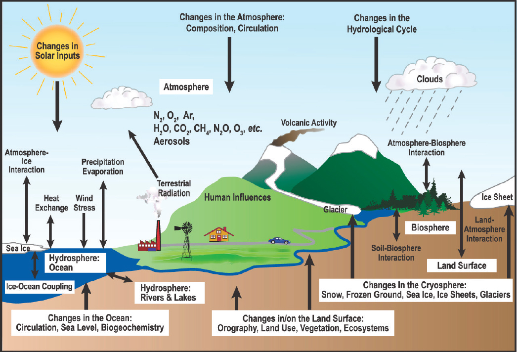
Earth system science—theory, observations, and modeling—of the coupled atmosphere-ocean-biosphere-cryosphere system (Figure 9.1)—has advanced significantly in recent decades. There is now a better recognition of the principal gaps in knowledge that need to be filled in order to understand and predict both the natural variability and the long-term human-induced changes occurring in the Earth system. Reducing uncertainties in our predictions of the changing Earth system will help realize numerous economic benefits (e.g., the ability to reduce costs in mitigation and adaptation strategies, provide increased security for the agricultural sector, and improve the overall health of society). Increasingly accurate quantification of variability, changes, trends, and extremes in the climate system, on time scales from seasonal to centennial and longer, will positively impact several societal sectors and provide sustained opportunities to improve quality of life, safeguarding both lives and property.
Beginning with a focus on the impacts of improved understanding of climate variability and change, the Panel on Climate Variability and Change: Seasonal to Centennial identified a number of priority science topics for which key satellite measurements, together with complementary measurements from other platforms, will make a significant scientific impact with corresponding societal benefits. Table 9.1 summarizes the panel’s scientific and application priorities, as addressed in its questions and the measurement objectives.
These climate topics and the measurements needed to address them (Table 9.2) crosscut through all aspects of our Earth system, such as weather and air quality (including extreme events), ecosystems, and hydrology. Many of the topics and questions accordingly lend themselves to consideration under the various crosscutting and integrating theme concepts identified by this decadal survey (e.g., water and energy cycles, carbon cycle, etc.). Crucial and often unique elements of measurements targeted for climate questions are (1) the need for continuity of measurements across multiple decades, (2) observations of a wide variety of
___________________
NOTE: This chapter was written by members of the Panel on Climate Variability and Change: Seasonal to Centennial and is provided for reference only. Any study finding or consensus recommendation will appear in Chapters 1-5, the report from the survey steering committee.
variables, and (3) a need for highly precise and accurate measurements. In Table 9.2, the highest priority science and application objectives are mapped to the Targeted Observables that will strongly contribute to addressing those objectives.1
Observation strategies to address the complexity of climate processes and their interactions in the Earth system require careful coordination and synergy among satellite and in situ measurement programs. This is a critical time for climate observations, as several National Aeronautics and Space Administration (NASA) climate-related satellite observation platforms are aging, pointing to a risk of shortfalls in crucial, societally relevant scientific information. A number of new techniques, measurement strategies, and observational technologies are now available for the production of new, cost-effective, and beneficial measurements, thus providing an invaluable opportunity to advance the science for improved understanding of the Earth system and societal benefits.
___________________
1 Not mapped here are cases where the Targeted Observables may provide a narrow or an indirect benefit to the objective, although such connections may be cited elsewhere in this report.
TABLE 9.1 Summary of Science and Applications Questions and Their Priorities
| Science and Applications Questions | Highest Priority Science and Applications Objectives (MI=Most Important, VI=Very Important) | |
|---|---|---|
| C-1 | How much will sea level rise, globally and regionally, over the next decade and beyond, and what will be the role of ice sheets and ocean heat storage? |
(MI) C-1a. Determine the global mean sea-level rise to within 0.5 mm/yr over the course of a decade.
(MI) C-1b. Determine the change in the global oceanic heat uptake to within 0.1 W/m2 over the course of a decade. (MI) C-1c. Determine the changes in total ice-sheet mass balance to within 15 Gton/yr over the course of a decade and the changes in surface mass balance and glacier ice discharge with the same accuracy over the entire ice sheets, continuously, for decades to come. (VI) C-1d. Determine regional sea-level change to within 1.5-2.5 mm/yr over the course of a decade (1.5 corresponds to a ~6000 km2 region, 2.5 corresponds to a ~4000 km2 region). |
| C-2 | How can we reduce the uncertainty in the amount of future warming of Earth as a function of fossil fuel emissions, improve our ability to predict local and regional climate response to natural and anthropogenic forcings, and reduce the uncertainty in global climate sensitivity that drives uncertainty in future economic impacts and mitigation/adaptation strategies? |
(MI) C-2a. Reduce uncertainty in low and high cloud feedback by a factor of 2.
(VI) C-2b. Reduce uncertainty in water vapor feedback by a factor of 2. (VI) C-2c. Reduce uncertainty in temperature lapse rate feedback by a factor of 2. (MI) C-2d. Reduce uncertainty in carbon cycle feedback by a factor of 2. (VI) C-2f. Determine the decadal average in global heat storage to 0.1 W/m2 (67% confidence) and interannual variability to 0.2 W/m2 (67% confidence). (VI) C-2g. Quantify the contribution of the upper troposphere and stratosphere (UTS) to climate feedbacks and change by determining how changes in UTS composition and temperature affect radiative forcing with a 1-sigma uncertainty of 0.05 W/m2/decade. (MI) C-2h. Reduce the IPCC AR5 total aerosol radiative forcing uncertainty by a factor of 2. One objective associated with this question was ranked Important (C-2e). See subsequent sections for details. |
| C-3 | How large are the variations in the global carbon cycle and what are the associated climate and ecosystem impacts in the context of past and projected anthropogenic carbon emissions? |
(VI) C-3a. Quantify CO2 fluxes at spatial scales of 100-500 km and monthly temporal resolution with uncertainty <25% to enable regional-scale process attribution explaining year-to-year variability by net uptake of carbon by terrestrial ecosystems (i.e., determine how much carbon uptake results from processes such as CO2 and nitrogen fertilization, forest regrowth, and changing ecosystem demography.)
Six objectives associated with this question were ranked Important (C-3b, C-3c, C-3d, C-3e, C-3f, C-3g). See subsequent sections for details. |
| C-4 | How will the Earth system respond to changes in air-sea interactions? |
(VI) C-4a. Improve the estimates of global air-sea fluxes of heat, momentum, water vapor (i.e., moisture), and other gases (e.g., CO2 and CH4) to the following global accuracy in the mean on local or regional scales: (1) radiative fluxes to 5 W/m2, (2) sensible and latent heat fluxes to 5 W/m2, (3) winds to 0.1 m/s, and (4) CO2 and CH4 to within 25%, with appropriate decadal stabilities.
Three objectives associated with this question were ranked Important (C-4b, C-4c, C-4d). See subsequent sections for details. |
| Science and Applications Questions | Highest Priority Science and Applications Objectives (MI=Most Important, VI=Very Important) | |
|---|---|---|
| C-5 | A. How do changes in aerosols (including their interactions with clouds, which constitute the largest uncertainty in total climate forcing) affect Earth’s radiation budget and offset the warming due to greenhouse gases? B. How can we better quantify the magnitude and variability of the emissions of natural aerosols, and the anthropogenic aerosol signal that modifies the natural one, so that we can better understand the response of climate to its various forcings? |
(VI) C-5a. Improve estimates of the emissions of natural and anthropogenic aerosols and their precursors via observational constraints.
(VI) C-5c. Quantify the effect that aerosol has on cloud formation, cloud height, and cloud properties (reflectivity, lifetime, cloud phase), including semidirect effects. Two objectives associated with this question were ranked Important (C-5b, C-5d). See subsequent sections for details. |
| C-6 | Can we significantly improve seasonal to decadal forecasts of societally relevant climate variables? |
(VI) C-6a. Decrease uncertainty, by a factor of 2, in quantification of surface and subsurface ocean states for initialization of seasonal-to-decadal forecasts.
Two objectives associated with this question were ranked Important (C-6b, C-6c). See subsequent sections for details. |
| C-7 | How are decadal-scale global atmospheric and ocean circulation patterns changing, and what are the effects of these changes on seasonal climate processes, extreme events, and longer term environmental change? |
(VI) C-7a. Quantify the changes in the atmospheric and oceanic circulation patterns, reducing the uncertainty by a factor of 2, with desired confidence levels of 67% (“likely” in IPCC parlance).
(VI) C-7c. Quantify the linkage between global climate sensitivity and circulation change on regional scales including the occurrence of extremes and abrupt changes. Quantify the expansion of the Hadley cell to within 0.5 degrees latitude per decade (67% confidence desired); changes in the strength of AMOC to within 5% per decade (67% confidence desired); changes in ENSO spatial patterns, amplitude, and phase (67% confidence desired). Three objectives associated with this question were ranked Important (C-7b, C-7d, C-7e). See subsequent sections for details. |
| C-8 | What will be the consequences of amplified climate change already observed in the Arctic and projected for Antarctica on global trends of sea-level rise, atmospheric circulation, extreme weather events, global ocean circulation, and carbon fluxes? |
(VI) C-8a. Improve our understanding of the drivers behind polar amplification by quantifying the relative impact of snow/ice-albedo feedback versus changes in atmospheric and oceanic circulation, water vapor, and lapse rate feedback.
(VI) C-8b. Improve understanding of high-latitude variability and midlatitude weather linkages (impact on midlatitude extreme weather and changes in storm tracks from increased polar temperatures, loss of ice and snow cover extent, and changes in sea level from increased melting of ice sheets and glaciers). (VI) C-8c. Improve regional-scale seasonal to decadal predictability of Arctic and Antarctic sea-ice cover, including sea-ice fraction (within 5%), ice thickness (within 20 cm), location of the ice edge (within 1 km), and timing of ice retreat and ice advance (within 5 days). (VI) C-8d. Determine the changes in Southern Ocean carbon uptake due to climate change and associated atmosphere/ocean circulations. Five objectives associated with this question were ranked Important (C-8e, C-8f, C-8g, C-8h, C-8i). See subsequent sections for details. |
| Science and Applications Questions | Highest Priority Science and Applications Objectives (MI=Most Important, VI=Very Important) | |
|---|---|---|
| C-9 | How are the abundances of ozone and other trace gases in the stratosphere and troposphere changing, and what are the implications for Earth’s climate? | The objective associated with this question was ranked Important (C-9a). See subsequent sections for details. |
NOTE: Important (I) measurement objectives are not shown, but are included in the text in subsequent sections of this chapter. For objectives that reduce uncertainty by a factor of 2 or 3, the uncertainty refers to that described in major recent scientific reports such as the Intergovernmental Panel on Climate Change (IPCC) AR5. Confidence ranges appear for some of the objectives, marking a desired level of quantification.
TABLE 9.2 Priority Targeted Observables Mapped to the Science and Applications Objectives That Were Ranked as Most Important (MI) or Very Important (VI)
| Priority Targeted Observables | Science and Applications Objectives |
|---|---|
| Aerosol Vertical Profiles | C-2g, C-2h, C-5a, C-7a |
| Aerosol Properties | C-2g, C-2h, C-5a, C-7a |
| Temperature, Water Vapor, Planetary Boundary Layer (PBL) Height | C-2b, C-2g, C-2h, C-4a, C-7a, C-7c, C-8a |
| Atmospheric Winds | C-2h, C-4a, C-5a, C-7a, C-7c |
| Radiance Intercalibration | C-2a, C-2b, C-2c, C-2h, C-5c, C-7c |
| Precipitation and Clouds | C-2a, C-2g, C-2h, C-5c, C-7a, C-7c |
| Ice Elevation | C-1c, C-8a, C-8b, C-8c |
| Mass Change | C-1a, C-1b, C-1c, C-1d |
| Greenhouse Gases | C-2d, C-3a, C-4a |
| Surface Characteristics | C-2h, C-3a, C-5a, C-8c |
| Ozone and Trace Gases | C-2g |
| Sea-Surface Height (SSH) | C-1a, C-1b, C-1d, C-4a, C-6a, C-7a, C-8a, C-8b, C-8c |
| Terrestrial Ecosystem Structure | C-2d |
| Ocean Ecosystem Structure | C-2d |
| Aquatic-Coastal Biogeochemistry | C-2d, C-5a |
| Snow Depth and Snow Water Equivalent (SWE) | C-7a C-8c |
| Soil Moisture | C-3a, C-5a, C-6a, C-7a |
| Salinity | C-6a, C-7a |
| Surface Deformation and Change | C-1c |
| Ocean Surface Winds and Currents | C-1d, C-4a, C-5a, C-6a, C-7a |
| Vegetation, Snow, and Surface Energy Balance | C-7a |
| Surface Topography and Vegetation | C-1c, C-7a |
The societal benefits derived from the improved observations associated with each objective include the improved health and well-being of the nation’s and world’s population and the global ecosystems, along with improvements in global economic and social infrastructure. Observations providing insights into variability and processes and observations providing continued monitoring of the Earth system are both important for assessing the risks associated with climate variations and trends. As improved climate information becomes available, the advancement of knowledge about the Earth system and reductions in uncertainties will allow improved analysis and detection of climate variations and trends, and this can be translated into improved information for vulnerability, mitigation, and adaptation assessments—information that can be used in planning and decision making by stakeholders.
INTRODUCTION AND VISION
Motivation
Climate is intricately intertwined in virtually every aspect of the environment and human activity, shaping ecosystems, societies, and their economies (Carleton and Hsiang, 2016). Climate sets the stage and continually influences the development of natural systems. Whether determining what crops to grow, how to secure freshwater, or where to seek food and fiber from the land and seas, the critical role of climate has long been recognized by civilizations that have flourished around the world. A desire to make the best use of our natural resources has motivated scientific research and observations to better understand what drives climate and to improve predictions of future climate conditions. Indeed, sustained investments in climate observations and scientific research have yielded widespread scientific and societal benefits.
Understanding of climate variation and change across seasons, years, decades, and centuries has improved significantly. The increased knowledge in recent decades has led to improved capabilities to predict regional probabilities for fair weather, extreme heat or cold, droughts, heavy rainfall events, sea-ice coverage, and other climate conditions. For example, several national and international initiatives to investigate and improve seasonal prediction have been launched, including the North American Multi-Model Ensemble (NMME; Kirtman et al., 2014), EUROSIP (Vitart et al., 2007), and the Sea Ice Prediction Network (SIPN). Although still early in the development process, these forecasts are already used by farmers to help decide what seed varieties to plant each year, by water managers to inform choices about reservoir levels, by the military and transportation sectors to guide Arctic operations, and by many others (NASEM, 2016).
Understanding of long-term climate drivers—including greenhouse gases (GHGs) and aerosols in the atmosphere, land use, and volcanic aerosols and solar variability—and how they affect climate across decades and centuries, has also advanced, allowing us to anticipate, mitigate, and prepare for shifts in climate conditions and their impacts. This knowledge is particularly important today, as the climate is in the midst of a significant worldwide transition. Global mean surface air temperature has increased by 1°C since 1901, and the past 3 years have been the warmest on record (USGCRP, 2017). Through careful observation, analysis, and modeling, a peer-reviewed assessment by the world’s scientists (IPCC WG1, 2013) concludes that “it is extremely likely that human influence has been the dominant cause of the observed warming since the mid-20th century,”2 with more than half of the observed increase in global average surface temperature caused by the anthropogenic increase of greenhouse gas concentrations (arising from burning of fossil fuels, cement production, deforestation, and agriculture) and other anthropogenic forcings together. Assessment of the projected climate change due to different emissions scenarios indicates that, with significant reduction in emissions of greenhouse gases, global average temperature increase could
___________________
2IPCC (2013) uses the following terms to indicate the assessed likelihood of an outcome or a result: extremely likely (>95 percent); likely (>66 percent).
be limited to 2°C by the end of the 21st century. With higher emissions scenarios, the annual average global temperature could reach 5°C or more by the end of the century compared to preindustrial times (USGCRP, 2017).
Global warming has impacts on many other parts of the climate system—for example, causing sea ice, glaciers, and ice caps to melt, sea levels to increase, and ecosystems to shift both on land and in the ocean. Some of these climate changes could be effectively irreversible, lasting hundreds to thousands of years, including increasing ocean acidification due to increases in carbon dioxide, sea-level rise, melting of land ice masses, and a reduction in permafrost coverage (IPCC, 2014). A changing climate implies risks to national and global security (food, water, conflicts, and migrations), to major economic sectors (agriculture, transportation, freshwater management, and multiple sectors relying on coastal infrastructure), and to unique and threatened terrestrial and marine ecosystems.
Climate change is now well recognized as a major scientific and societal challenge (e.g., NRC, 2011, 2012; IPCC, 2007, 2014; Melillo et al., 2014; USGCRP, 2017). Reflecting global climate change concerns, there have been concerted efforts by the world community to negotiate and make an advance toward agreements on emissions.
Space-based observations of Earth have been critical for advancing our understanding of global climate processes, climate variations and trends (see Box 9.1).
Despite the significant contributions of space-based observations to climate science, the climate system is not yet adequately measured, as there is no long-term commitment to measure all important variables globally, thereby limiting progress in research and applications. For example, accurate climate prediction relies in part on data used to initialize the forecast, yet many critical variables are not measured routinely (e.g., snow depth on sea ice, sea-ice thickness, soil moistures in the root zone, seafloor bathymetry, Antarctic ice thickness). Many of these variables can be measured only on a global scale economically by satellites; others require investments in in situ measurements. Predictions beyond the decadal scale are essentially limited by uncertainties (and associated modeling deficiencies) in aerosol radiative forcing, in climate feedbacks such as those involving clouds (IPCC WG1, 2013), in ocean and ice variability, and in the evolution of carbon and other biogeochemical and ecosystem cycles (IPCC; U.S. Global Change Research Program [USGCRP]; Melillo et al., 2014). The 2007 Decadal Survey for Earth Science and Applications from Space called for a major increase in NASA Earth science investments in these areas, but increases were realized in only some areas of climate science. The international Global Climate Observing System (GCOS) Implementation Plans (WMO, 2016) have been very effective at defining existing observations that are needed for long-term climate monitoring. But the GCOS plan has been much less effective at planning for needed improvements in the observations to address climate science challenges.
Recent studies have estimated just how valuable improvements in climate information would be to the global economy. For example, narrowing scientific uncertainty in climate sensitivity using an improved climate observing system and modeling could be worth as much as $10 trillion U.S. dollars to the world economy3 (Cooke et al., 2014, 2016a, 2016b; Hope, 2015). The reduced scientific uncertainties enable improved economic decisions on the relative balance of climate change mitigation versus adaptation. At this value the cost of tripling the current level of global climate research for 30 years would provide a $50 return for every $1 invested (Cooke et al., 2014).4 Even a factor of 5 uncertainty in this economic analysis would lead to a robust return on investment that would range from 10:1 to 250:1.
___________________
3 Economic value is specified as either the net present value or the real option value of future economic benefits at a 3 percent discount rate, the nominal value specified in the U.S. Social Cost of Carbon Memo (Interagency Working Group on SCC, 2010). The economic value is an expected value of a large ensemble of simulations using the current range of climate sensitivity uncertainty specified in IPCC (2013).
4 Current global annual investment in climate research (e.g. observations, analysis, and modeling) is approximately $5 billion U.S. dollars (Cooke et al., 2014). Tripling that level of investment to achieve an observing system optimized for climate research would
Vulnerabilities associated with severe seasonal anomalies make yet another pressing case for sustained long-term observations and improved predictions. For instance, the cost of seasonal uncertainty to the agricultural sector is between 20 and 40 percent of the average gross margin, with an expected value of forecast information between $1 and $17/ha depending on the crop. Improved accuracy and longer lead-times could increase this value (e.g., Meza et al., 2008).
The present decadal survey provides guidance on the highest priority observations needed within NASA’s current budget profile, as well as a more rigorous and complete set of quantified climate science
___________________
cost an additional $10 billion per year. Return on investment assumes a 30-year commitment to such an enhanced climate research effort, and applies the same 3 percent discount rate used for the value of information (VOI) estimates.
objectives that could be used as the basis for a comprehensive climate observing system. This system could be realized as a combination of U.S. and international observations similar to the current international investment and collaboration on global weather observations—for example, World Meteorological Organization (WMO), GCOS—and it would take advantage of developments in active remote sensing technology—for example, backscatter lidar (Cloud-Aerosol Lidar and Infrared Pathfinder Satellite Observations [CALIPSO]/Cloud-Aerosol Lidar with Orthogonal Polarization [CALIOP]), backscatter radar (CloudSat, Global Precipitation Measurement [GPM]), high spectral resolution lidar and Doppler radar (Earth Cloud Aerosol and Radiation Explorer [EarthCARE])—as well as passive remote sensing capability—for example, greatly improved spectral and spatial resolution and higher accuracy calibration methods. Careful attention to calibration and ground truth will be needed to ensure cross-mission continuity and comparability over decadal time scales.
The need for improved climate observations has become more urgent today, as the extent and pace of climate change increases and the value of improved information is more apparent. More significantly, the “nonstationarity” of climate has become evident (e.g., Milly et al., 2008). Climate science has moved from the vast scope of “unknown unknowns” of the 1980s to many “known unknowns” of the present (e.g., IPCC WG1, 2013). Given the societal relevance of climate variations and the inherent value (economic, human health and welfare, human safety and security) of predicting them before they occur, the current deficiencies in measurements that limit effective monitoring and prediction of these variations need to be addressed through the formulation and implementation of science-based global climate observing strategies using innovative technology. Considerable investment in climate measurement is needed now; the return on the dollar from such investment could be tremendous and long-lasting in the decades to come (Weatherhead et al., 2017).
Science and Applications Challenges
Earth system science—theory, observations, and modeling—of the coupled atmosphere-oceans-biosphere-cryosphere system (Figure 9.1)—has advanced significantly in recent decades. There is now a better recognition of the principal gaps in knowledge that need to be filled in order to understand and predict both the natural variability and the long-term human-induced changes occurring in the Earth system. Strategies for observing, and quantifying, the mechanisms driving climate phenomena and the agents producing climate change are more firmly grounded owing to advances in the prior decade. Developments arising from both space-based and in situ observations over the past decades have revealed important insights into the complexity of the interactions occurring between the atmosphere, ocean, land, and cryosphere, as well as in the trends in key variables (e.g., surface temperature, heavy precipitation, Arctic summertime sea ice, northern hemisphere snow cover).
There has been steady progress from qualitative concepts to quantitative climate science over the past decade by virtue of advances in both observations and numerical modeling. In turn, this has made clear the need for further quantitative climate information through advances in the observation of key variables that are critically relevant for societal objectives. Currently recognized scientific uncertainties in climate (e.g., see IPCC WGI, 2013) strongly indicate the critical need to measure continuously an array of variables, for many decades, in order to ensure a comprehensive understanding of climate forcings and feedbacks, global and regional climate sensitivities, natural variations, and forced changes. There is an equally strong and compelling requirement to quantify trends, taking into account the processes influencing the Earth system, and including a better accounting of uncertainties. For instance, difficulties persist in trying to narrow the bounds on the estimate of Earth’s climate sensitivity. Reducing the uncertainty in this parameter will require global measurements of key variables—for example, aerosols, clouds, radiation, ocean heat
uptake, and related process studies involving the atmosphere, oceans, biosphere, and cryosphere. For the next decade and beyond, the measurement imperatives include (1) global climate observations, contributing to assessments of the rapidity of change in essential climate variables (e.g., frequency and severity of extreme events); (2) advancing the scientific frontiers using the upcoming decade’s observations of the climate system, and characterizing especially the societally relevant changes on continental-to-regional scales; and (3) an emphasis on continuity so that gaps in observations that would preclude or impair scientific understanding and societal benefits are avoided. Especially with regard to the estimation of trends in the key variables of concern to society, focus is needed on obtaining higher levels of precision, and planning for redundancy and cross-validation of measurements.
In deciding which observations are to be made, and in using those observations, the increasing complexity of models and the attendant observational data requirements must be taken into account. These include growing demand for measurements of a vast range of space-and-time-dependent variables on which the models need to be tested and improved. Moreover, observational data are needed now on a widening set of Earth system variables—for example, expanding from the details of the physical climate system to include biogeochemistry and ecosystems. A crucial element is gaining improved knowledge of the processes that govern the Earth system. Additionally, accurate observational data sets are needed to initialize and verify models and for model-based predictions and projections.
The systematic establishment of the scientific basis of climate (e.g., NRC 2012, 2016; IPCC, 2013), together with the ever-increasing evidence that climate is not stationary but instead comprises variations and changes, creates a sound rationale for, and compellingly justifies, continuous global measurements of key climate variables. Analyses of the measurements in turn will continue to improve socioeconomic decision making for many sectors, providing quantitative climate information and uncertainties. There is an even greater demand now for credible global and regional climate data to perform impacts and vulnerability assessments, and in mitigation and adaptation planning that links essential global weather and climate information to serving, protecting, and enhancing property and human life. In effect, there are a multitude of users with differing requirements, rendering it a huge challenge to address all the needs effectively. Societal sectors especially benefiting from climate information in the present and future include agriculture, fisheries, water management, ecosystem management, coastal management, and air quality management, as well as management of long-term transportation and energy infrastructure.
The measurement requirements for long-term monitoring (over time scales of decades) of many climate parameters are challenging and necessitate rigorous calibration/validation across missions. The complexity of climate processes, and the interactions among them, motivates careful coordination of satellite and in situ measurement programs. Simultaneous measurements of multiple variables from space and in situ are needed to produce a reasonably complete and consistent picture of Earth system features and to support transparent estimates of uncertainty in measurement and understanding. It is critical that the focus on climate quality observations be strengthened and sustained—in particular, satisfying the GCOS observing principles (NRC, 2007; Trenberth et al., 2013; Simmons et al., 2016; WMO, 2016; Weatherhead et al., 2017). Collaboration with international space agencies will be important, involving access to calibration, processing, algorithm, and data systems (i.e., some measurements may exist on other platforms but are not accessible, or it is not known how they are calibrated).
Last, continuity of observations of critical climate variables for “seamless” (in time scale) understanding and quantification of climate change is a fundamental scientific objective. Such continuity will allow the assessment of the robustness of trends determined for climate variables that are superimposed on the naturally varying system. Thus, sustaining climate observations will need to be an important element of the decadal survey. This will also challenge the current paradigm in the lack of a single agency “owning” the entire end-to-end climate observations and monitoring missions.
A wide range of NASA satellite sensors relevant to climate, including those measuring variables that plausibly have a trend against the backdrop of variations, are aging, and this threatens to produce gaps in the measurement record that would reduce, and perhaps even preclude, our ability to quantify critical trends (NRC, 2015). It is imperative to find ways to sustain key measurements in the face of aging platforms and to rigorously link measurements across missions. Emerging new technologies can be used to avoid these gaps and improve the accuracy of critical climate observations (e.g., aerosols, clouds, radiation balance, temperature and humidity, ice-sheet dynamics). Strategic investments are needed in infrastructure for “ground-truthing” that can link satellite measurements to internationally recognized calibration scales and that can serve multiple missions.
Opportunities
The next decade of space-based climate observations presents opportunities for exciting breakthroughs that would build on the progress of the past decade. As discussed later, these opportunities build upon (1) improvements in understanding of climate processes; (2) advancements in data science and the resulting ability to produce better reanalyses; (3) the use of model projections in concert with advanced instrument capabilities; (4) enhanced coordination among funding agencies; and (5) more widespread recognition and sophisticated tools to ensure continuity of observations.
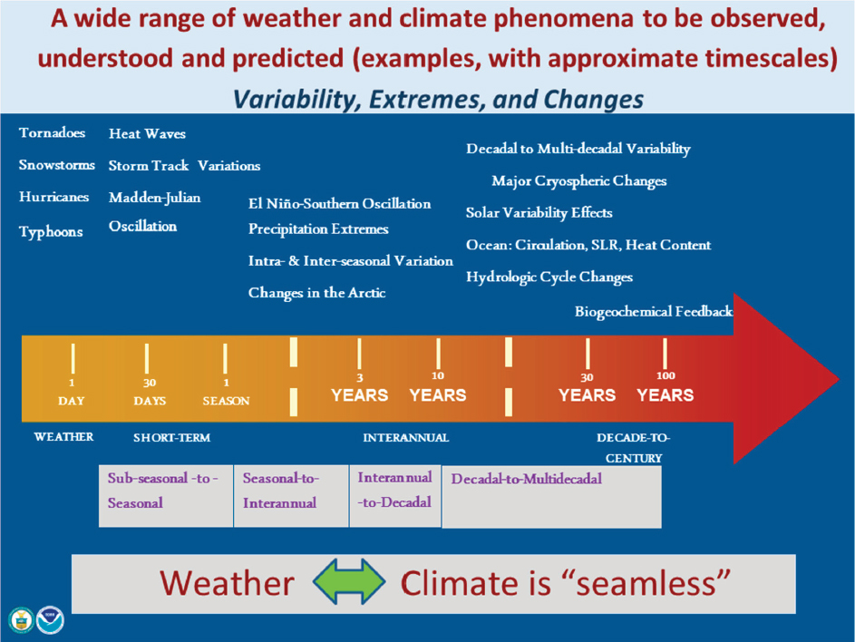
The first is an improved understanding of the important climate processes and phenomena spanning the short to the long time scales (a few examples are illustrated in Figure 9.2), which have to be understood and predicted, including climate variability, changes, and extremes.
This leads to a sharper realization of the key variables to be monitored for characterizing and quantifying variations/changes of environmental consequence to society, as well as the need for continuity in these measurements. Over the past decade there has been an increased recognition of impact-relevant physical, chemical, dynamical, and biogeochemical processes governing climate (e.g., IPCC AR5; Melillo et al., 2014; WMO, 2014). New insights into phenomena of possible abrupt or irreversible changes in the climate system have also elevated the seriousness and invaluable utility of global observations for resolving key climate questions directly related to societal benefits (NRC, 2013). Further, increasing fidelity of climate models, in conjunction with space-based and other global observations over the past decade, has given rise to insights into processes spanning time scales from weather to climate. This has laid the foundation for a more quantitative understanding of critical mechanisms through comprehensive and sustained observations, which in turn can lead to increased certainty of our understanding of the central challenges—for example, variation and trends in climate variables, climate feedbacks and sensitivity, rate of regional sea-level rise, weather-to-climate information on the mean and extremes, and so on. In this regard, further development and expanded use of Climate Observing System Simulation Experiments (COSSEs) are needed to better understand the utility and quality of the required observations for climate change (see NRC, 2015).
Second, improved data management, data initialization, and data assimilation techniques used with global numerical Earth system models have supported improved “reanalysis procedures,” which complement and augment space-based and other observational data to estimate the state of the Earth system. Using mathematically optimized techniques and a high-level understanding of Earth system physics, such reanalyses “fill in the gaps” of the measurement record with reasonable confidence, leading to a picture of the Earth system that is comprehensive in both space and time. Importantly, these reanalyses can also ingest a wide variety of measurement types, so that the resulting complete Earth system picture becomes a reflection of all of them. The modeling framework allows satellite-based measurements of one component of the system to improve estimates of remote quantities (e.g., the assimilation of space-based sea-surface temperature measurements can have an impact on the reanalysis continental temperature product). Most
current reanalyses focus on the ocean or atmosphere components separately, although studies have pointed to new methods involving multiple components of the Earth system—for example, ensemble coupled atmosphere-ocean data assimilation (Zhang et al., 2005) and coupled physical-biogeochemical data assimilation (Verdy and Mazloff, 2017). The future of reanalysis, however, lies in the Integrated Earth System Analysis (IESA), which involves assimilating data into a fully coupled complete climate (ocean-land-atmosphere-cryosphere) system to ensure the highest possible self-consistency amid all of the analysis-enhanced climate variable estimates.
The third element is the wider set of opportunities made possible by (1) state-of-the-science model predictions and projections on time scales ranging from weather to climate, based on observations and future scenarios of emissions of important atmospheric constituents; and (2) the advances in instrument technology and remote sensing strategies—for example, more accurate, cheaper, and lighter instrumentation is available now, and methods are available to quantify the consequences of using this technology in numerical models. Projections and predictions of the future state of the Earth system, together with the rapid advances in technology, ensure that the desired measurements to monitor the evolution of the system across
various space scales can be performed to a high degree of accuracy. For example, NASA satellites provide a unique global view of the climate system from the surface to the top of the atmosphere and beyond, with the potential for large improvements in resolution and accuracy over current methods due to improved measurement techniques and sensors. Improved surface-based measurements and field campaigns are enhancing global observations from satellites, often with higher temporal and spatial resolution than can currently be observed from space and capturing the Earth system complexity better than before. Improvements in technology for subsurface ocean observations through autonomous vehicles are also shaping our ability to determine the ocean state more completely than in the past. Together with strategic steps in ocean observations that have been shaped through U.S. (NOAA)-led international partnerships—in particular, Argo (and Deep Argo) floats complemented by the potential of biogeochemistry sensors (Biogeochemical-Argo) deployed worldwide (Riser et al., 2016)—there now emerges the ability to quantify the role of the ocean in the Earth system with enhanced perspectives of ocean-atmosphere interactions—for example, subseasonal-to-decadal prediction, energy and hydrologic cycle variations linked to climate variations and change, and heat and CO2 exchange between the atmosphere and ocean and storage of these quantities in the ocean (e.g., the Southern Ocean Carbon and Climate Observations and Modeling [SOCCOM] Project is performing measurements of carbon and other variables in the Southern Ocean;5 carbon-climate feedback is one of the World Climate Research Programme [WCRP] Grand Challenges involving the Earth system6).
Fourth, improved synergies being developed among federal agencies for observing/monitoring the atmosphere, the oceans, the climate and ecosystems, and the social and economic implications, are leading to important joint undertakings (e.g., involving National Oceanic and Atmospheric Administration [NOAA], NASA, Department of Energy [DOE], Environmental Protection Agency [EPA], National Geospatial-Intelligence Agency [NGA]). These are creating new observational opportunities through interagency common priorities. Collaboration with new international long-term observation programs such as the European Space Agency (ESA) Copernicus/Sentinel satellites are adding complementary observational platforms, affording an increase in observing instruments. Synergies between programs (e.g., Committee on Space Research [COSPAR]) and space agencies (e.g., Japan Aerospace Exploration Agency [JAXA], Indian Space Research Organization [ISRO], ESA, Canadian Space Agency) are notably augmenting the understanding of the global climate system.
Fifth, a wide range of recent reports has recognized the critical need for continuity of climate records (NRC, 2007; IPCC, 2013a; NASEM, 2015; WMO, 2016). Most climate observations lack the inherent absolute accuracy required to survive even short 1-year gaps without seriously degrading the climate record (NRC, 2007; Trenberth et al., 2013; NASEM, 2015). Continuity is especially challenging for satellite records where instruments have widely varying lifetimes on orbit. A range of recently developed analysis tools make it much easier to consider the statistical risk of satellite record gaps (Loeb et al., 2009), as well as the amount of degradation to climate records should gaps occur (Leroy et al., 2008; Wielicki et al., 2013; NASEM, 2015; Shea et al., 2017). Last, new instrument technologies have been developed to provide international standard traceable spectrometers in orbit to enable accurate calibration across climate record gaps for reflected solar and thermal infrared climate instruments (NRC, 2007; Wielicki et al., 2013; NASEM, 2015). The Global Space-Based Intercalibration System (GSICS) has requested orbiting climate accuracy reference spectrometers to serve as the basis for their intercalibration system to enable reducing the effect of gaps on climate records, as well as to improve the consistency and accuracy of current intercalibration standards for satellite instruments (Goldberg, 2011). A similar approach is envisioned in
___________________
5 See Princeton University, Southern Ocean Carbon and Climate Observations and Modeling (SOCCOM) Project, “Overview,” https://soccom.princeton.edu/content/overview.
6 See World Climate Research Programme, “WCRP Grand Challenges,” https://www.wcrp-climate.org/grand-challenges/grand-challenges-overview.
the Committee on Earth Observing Satellites (CEOS)/World Meteorological Organization (WMO)/ Committee for Meteorological Satellites (CGMS) joint study on an Architecture for Climate Monitoring from Space (Dowell et al., 2012). Understanding of the continuously evolving Earth system (depicted in Figure 9.1) crucially requires continuity of observations. Furthermore, continuous measurements of atmospheric, oceanic, biospheric, and cryospheric variables are essential for sustained predictions of the system from the weather to climate time scales. A continuum of time scales also meets the urgent need for the U.S. weather and climate communities to successfully address “seamlessness” in weather-to-climate forecasting (e.g., NRC, 2012), taking into account not only the “average” weather or climate but also the occurrence of the extremes (e.g., the “tails” of the probability distribution function of atmospheric and ocean states; see IPCC, 2013, Technical Summary).
Relevant Climate Topics
A number of critically important and currently unresolved/unanswered science and societally related questions rose to the top of the priority list in the panel’s deliberations. The quantified Earth science/application objectives producing the Most Important priorities are associated with the following questions.
C-1: Sea-level Rise: Ocean Heat Storage and Land-Ice Melt
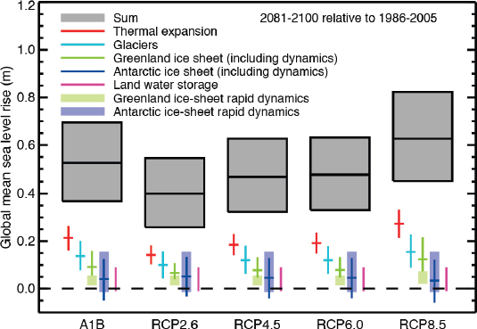
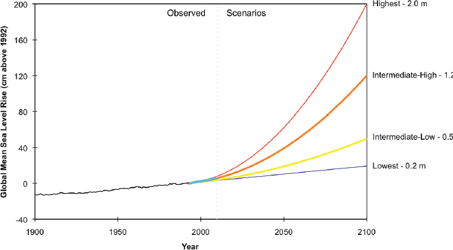
The rise of the global mean sea level is an integrated response to the change of a major part of the Earth system caused by the warming of the planet. The change of the global mean sea level is now well determined from spaceborne measurements with sufficient accuracy to evaluate not only the rate of change but also the various factors affecting the change (Cazenave et al., 2014; Leuliette and Nerem, 2016). On the basis of observations and modeling studies confidence in projections of global-mean sea level has improved (IPCC WG1, 2013). However, significant uncertainties remain, particularly related to the magnitude and rate of the land ice-sheet contribution for the twenty-first century and beyond, the regional distribution of sea-level rise, and the regional changes in storm frequency and intensity of relevance for coastal impacts. Shown in Figure 9.3 are the IPCC WG1 (2013) estimates of the range of global sea-level rise under various emission scenarios and the contributions from the various sources such as ocean warming and glacier melting. Predicting the geographic pattern and rate of sea-level rise is a grand challenge relevant to coastal infrastructure and human habitation. The need for reliable information on future sea-level rise is further underscored by the increase in flood frequency during high tides in U.S. coastal cities (Sweet and Park, 2014; Sweet and Marra, 2015), which impacts the health of coastal communities.
The rate of future sea-level rise is highly uncertain, especially in terms of upper bounds in potential sea-level rise (Pfeffer et al., 2008; Parris et al., 2012; Sriver et al., 2012). These new studies have placed the upper bound of the rise of the global mean sea level by 2100 from 1 m (IPCC AR5) to 2.5 m (NOAA, 2017). Maintaining, and improving, the sea-level measurement system is crucial for monitoring and predicting the future sea-level rise, which will potentially alter coastlines and affect the security and prosperity of society, particularly with half of the world’s population living close to the coast.
Since the industrial revolution the extra heat from greenhouse gas warming is mostly (>90 percent) stored in the ocean (Cheng et al., 2017). The rate of the change of ocean heat storage is of crucial importance to the prediction of future climate and sea level. The global ocean heat gain over the 0-2000 m layer during 2006-2013 was estimated to be 0.4-0.6 W/m2 (Roemmich et al., 2015). This estimate was based on direct measurement by the Argo array. It shows a large uncertainty. Over the course of the twenty-first century, as the global oceans warm, it will be important to monitor both (1) the warming of the surface, especially in the subtropical and tropical regions; and (2) penetration of heat into the deeper ocean, espe-
cially in the Southern Ocean (IPCC, 2013). A combination of spaceborne and in situ observing systems is required to accurately determine the change of global ocean heat storage (Llovel et al., 2014; Fu, 2016).
C-2: Climate Feedbacks and Sensitivity
A key reason for the well-known uncertainty in climate change projections is the fact that the models making the projections do not fully agree on how sensitive various facets of the climate system (e.g., clouds and their radiative feedbacks) are to radiative forcing of the climate system. Radiative forcings can occur due to natural factors, such as solar irradiance and emissions from volcanic eruptions, or arise due to human influences—for example, greenhouse gas and aerosol emissions and land use changes. The “sensitivity” refers to how the global and regional systems respond to changes in these factors. Physical processes in the climate system produce feedbacks that control the warming of Earth in response to increases in the well-mixed greenhouse gases. Further complicating the matter, the magnitude and sign of the radiative forcing (RF) of climate measured as the perturbation in radiative flux change at the tropopause, due to anthropogenic aerosols, are highly uncertain (Smith and Bond, 2014), as shown in Figure 9.4. The radiative cooling of climate due to anthropogenic aerosols (blue boxes, Figure 9.4) have and could continue to offset a portion of the warming due to greenhouse gases (lower error bar of box labeled Total Anthropogenic) or not (upper error bar, Total Anthropogenic). While observations and model-based studies have contributed to a better understanding of water vapor and cloud feedbacks, there continues to be uncertainty as to the
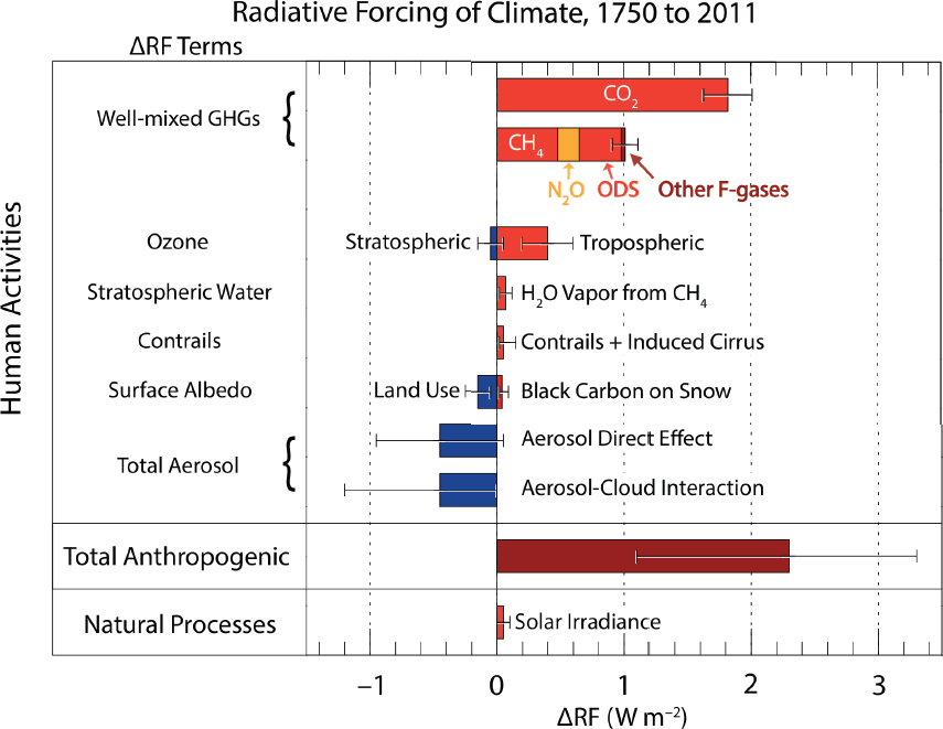
sign and magnitude of the feedbacks due to clouds. This, in turn, leads to an unacceptably large range in the value of the climate sensitivity.
The influences on precipitation due to the anthropogenic emissions, especially relative to natural variability, are uncertain in the model projections (IPCC, 2013). While climate models generally agree on the projected increase in precipitation in the twenty-first century over the high latitudes, they can disagree on even the sign of change in the low to midlatitudes. Thus, hydrologic cycle-related observations also must be made for a complete understanding of both thermal and hydrologic feedbacks in the surface-atmosphere response to radiative forcings.
Very Important and Important goals were also identified to address the following questions.
C-3: Carbon Cycle, Including Carbon Dioxide and Methane
Changes in radiative forcing arising from greenhouse gas emissions, principally CO2 and CH4 (see Figure 9.4), have been and will likely continue to be the most important driver of climate change in the twenty-first century. The land biosphere and the ocean together currently absorb over half of the CO2 emitted by human activities. Understanding climate-carbon cycle feedbacks—for example, release to
the atmosphere of carbon stored in vulnerable reservoirs such as permafrost, frozen methane hydrates, or tropical forests—in a changing climate has been recognized as an important goal by the IPCC WG1 (2013). Additionally, methane is a primary sink for the hydroxyl radical, and thus critically important for atmospheric chemical processes and global air quality due to its regulation of the oxidation capacity of the atmosphere.
C-4: Atmosphere-Ocean Flux Quantification
The current inability to quantify air-sea fluxes is a critical source of uncertainty in closing the global energy, water, and carbon cycles (e.g., L’Ecuyer et al., 2015; Rodell et al., 2015). The interface between atmosphere-ocean, atmosphere-land, and ocean-ice systems represents the coupling of Earth system components operating physically on different time scales such that the interactions between them lead to variations and changes in the states of the climate system. The exchange of heat, moisture, and momentum between the ocean and atmosphere helps drive the atmospheric circulation, contributes to precipitation variability, and modulates the heat storage of the ocean. The carbon exchange between the ocean and atmosphere represents one of the significant unknowns regarding uptake by the surface and the ability of the Earth system to store carbon outside of the atmosphere. It thus becomes important to quantify these accurately.
C-5: Aerosols and Aerosol-Cloud Interactions
The nature of these interactions has a critical—and largely unquantified—impact on climate sensitivity to anthropogenic emissions. An additional critical factor is the influence of the radiative forcings on regional precipitation, with indications that the effect of anthropogenic aerosols could be comparable to that of the greenhouse gases (e.g., Asian monsoon, Bollasina et al., 2011; northern hemisphere precipitation, Polson et al., 2014). Progress on this long-known limitation (e.g., Anderson et al., 2003) has been slow, due to the complexity of the problem and the difficulty of representing these processes within global models.
C-6: Seasonal-to-Interannual Variability and Predictions
Improved seasonal forecasts, including, for example, drought forecasts and sea-ice forecasts and particularly forecasts of the potential for weather extremes governed by atmospheric and ocean states, will lead to direct economic benefits through improved water management, agricultural planning, and so on, yet are currently limited by inaccuracies in forecast initialization arising due to uncertainties in observations and in the model physics used to evolve the states forward (NRC, 2016).
C-7: Decadal-scale Changes and Extremes in Atmospheric and Oceanic Circulation Patterns
Changes in large-scale circulation regimes could have substantial impact on regional weather extremes (droughts, flooding, hurricanes, etc.). Such changes can arise due to the variability in ocean states or to the forcing posed by greenhouse gases, aerosols, and other anthropogenic factors as well as natural (solar, volcanic aerosol) radiative perturbations (Yang et al., 2013). The nature of such circulation changes, however, is very uncertain (Abraham et al., 2013) and is subject to the same challenges as seasonal-to-interannual predictability.
C-8: Causes and Effects of Polar Amplification
Improved understanding of the connection between polar processes and global climate would help improve seasonal-to-decadal prediction. The Arctic and Antarctic are expected to respond relatively quickly to global climate change, and Arctic warming may already be associated with significant impacts on midlatitude weather (Richter-Menge et al., 2016). In addition, land-ice changes can affect global-to-regional sea-level rise, glacier changes will affect river hydrology and freshwater supply for large populations, while thaw of the large permafrost carbon pool will affect the global carbon cycle. Observations and research are necessary to quantify how the expansion of open water areas from Arctic sea-ice loss and large reductions in hemispheric snow cover extent amplify Arctic warming (e.g., 2-3 times more than the global-mean currently), and how this in turn is correlated with changing atmosphere and ocean conditions in North America including sea-level rise. In the Antarctic the effect of the ozone hole and the increased concentration of greenhouse gases in Earth’s atmosphere has caused a strengthening of the westerlies and polar contraction of the winds that can affect sea-ice extent and land-ice melt in a significant way (Thompson et al., 2011; Spence et al., 2014), and may have exerted an influence on the southern hemisphere ocean circulation (Solomon et al., 2015).
C-9: Ozone and Other Trace Gases in the Stratosphere and Troposphere
Due to the success of the Montreal Protocol, which was enabled by space-based and other observations and accompanying model studies, the ozone layer is on course for recovery from prior depletion caused by the buildup of ozone depleting substances (ODSs). The pace and thickness of the ozone layer recovery will be dictated by future evolution of GHGs such as CH4 and N2O (Ravishankara et al., 2009; Revell et al., 2015), in addition to ODSs. Since the climate, particularly in the southern hemisphere during summer (Polvani et al., 2011), has been influenced by prior depletion of the ozone layer, the anticipated ozone recovery could cause a further change. Changes in the distributions of radiatively active trace gases such as ozone and H2O in the upper troposphere and lower stratosphere have also been shown to influence the global climate (Gettelman et al., 2011; Riese et al., 2012).
Together, these questions, the needs and the purposes served by addressing them, and their associated goals, define the measurement objectives identified by the panel.
PRIORITIZED SCIENCE OBJECTIVES AND ENABLING MEASUREMENTS
Rationale
The following questions were used as a basis for determining the scientific rationale for each of the key climate objectives discussed here: What is the unresolved science question being addressed, why is it important, and how is it societally relevant? How does meeting the objective build upon, substantiate, or add innovatively to the knowledge about processes, variations, and change in the Earth system arising from historical measurements? What gaps exist in our current set of measurements? Why are the measurements important today, and what will be needed in the decades ahead? What are the principal climate uncertainties to be reduced—in processes, in understanding, and in making predictions—that lead to tangible, measurable gains for society? It should be noted that a complete weather and climate observing system could address many more scientific unknowns and could provide many more benefits than are addressed here; however, given current budgetary constraints, the panel realized that such a complete system is untenable and therefore prioritized the objectives to be met and the measurements needed to meet them.
Societal Benefit
Examples of the societal benefits derived from the improved observations associated with the following objectives are detailed within the discussion of each objective; these benefits include the improved health and well-being of the world’s populations and the world’s ecosystems, and improvements in global economic and social infrastructure. Observations providing insights into variability and processes, and observations providing continued monitoring of the Earth system are both important for assessing the risks associated with climate variations and trends. As improved climate information becomes available, the advancement of knowledge about the Earth system and for reducing its uncertainties will allow improved detection of climate variations and trends. This can be translated into improved information for vulnerability, mitigation, and adaptation assessments—information that can be used in planning and decision making by stakeholders.
The information needed for the science and the associated societal advances will require continuity (over decades) in the space-based observations, complemented by critical surface and other in situ measurements. Critical analysis of the measurements as well as combining the data within a state-of-the-science reanalysis system will provide a comprehensive and quantitative picture of a broad suite of climate variables; using this information to evaluate and improve forecast models will in turn provide valuable predictions of important climate processes, variables, and risks.
It should be explicitly noted that socioeconomic scenarios that span the full range of possible futures (e.g., futures that depend on varying emissions trajectories for greenhouse gases and global mitigation policy implementation) will frame the context for the evaluation of the societal benefits. The range adds to the uncertainties that exist because of gaps in our current understanding of the physical system (e.g., range of climate sensitivities due to emissions of greenhouse gases, sensitivity of sea-level rise to thermal expansion of water, and ice-sheet dynamics due to changing ocean and air temperatures).
Prioritization Based on Scientific Importance and Societal Significance
All of the scientific questions that were discussed by this panel and reported here were deemed to be of high significance from the perspectives of both science and societal benefit; they are of value in improving predictions and reducing uncertainty across a wide variety of climate phenomena and processes, and should be the focus of climate observations over the coming decade.
Objectives framed by the panel are associated with science questions spanning the subjects listed here. As articulated by the Steering Committee, the range of questions in the context of this decadal survey has been partitioned into Most Important, Very Important, and Important categories.
The subjects that yielded Most Important objectives are as follows:
- C-1. Sea-level rise: ocean heat storage and land-ice melt
- C-2. Climate feedbacks and sensitivity
Other subjects that yielded Very Important and Important objectives are listed here:
- C-3. Carbon cycle, including carbon dioxide and methane
- C-4. Atmosphere-ocean flux quantification
- C-5. Aerosols and aerosol-cloud interactions
- C-6 and C-7. Seasonal-to-decadal predictions, including changes and extremes
- C-8. Causes and effects of polar amplification
- C-9. Ozone and other trace gases in the stratosphere and troposphere
C-1: Sea-level Rise: Ocean Heat Storage and Land-Ice Melt
Motivation
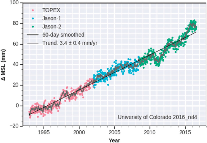
The rise of the global sea level represents an integrated response of the Earth system to the change of climate forced by increased heat stored on the planet. The two main contributors to sea-level rise are increased ocean heat storage, which causes thermal expansion, and melting of land ice (glaciers and ice sheets), which increases ocean mass. The projection of future sea-level rise, especially its geographic pattern in the coastal regions, is a grand challenge facing society. Before the satellite era, the rise of global sea level since the Industrial Revolution was measured using data from sparsely located tide gauges (Douglas, 2001). Over the 20th century, there was a total rise of ~20 cm, with an average rate of 1.7 mm/yr (IPCC WG1; Church et al., 2013). Since the 1990s systematic monitoring by satellite observations has enabled a more accurate assessment, indicating an acceleration in the rate of global sea-level rise to ~3.4 mm/yr over the past two decades (Figure 9.5). This rate is about one-third of the rate observed during the deglaciation some 10,000 years ago (IPCC, 2013).
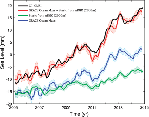
Over the past 15 years, simultaneous global observations of the sea-surface height from satellite altimetry (e.g., Jason series and Cazenave et al., 2017), ocean mass from satellite gravimetry (Gravity Recovery and Climate Experiment [GRACE]), and ocean density from Argo floats have made it possible to measure and partition the global sea-level change in terms of ocean warming and mass changes. This data set provides an overdetermined system for cross-comparison of the closure of the sea-level budget to estimate its uncertainty (Leuliette and Willis, 2011). The Argo network provides estimates on the thermal expansion contribution to sea-level change for comparison with the difference of the altimetry and GRACE measurements. Such analysis has shown that we are able to determine the change of the rate of global sea-level rise
to within 1 mm/yr (1-sigma) evaluated over the course of one decade (NRC, 2015; Fu, 2016). A decade is considered a minimum duration over which an estimate of the rate of sea-level change is relevant to the effects of climate change. This rate of sea-level change over a decade is comparable to the level of sea-level acceleration over the past 50 years (Church and Clark, 2013), representing the benchmark of the signal of sea-level change resulting from climate change in the coming decades. Therefore, a priority measurement objective should be to determine the global mean sea-level rise to within 1 mm/yr over the course of a decade with 95 percent confidence. Assuming Gaussian statistics, 1 mm/yr corresponds to two standard deviations of the measurement uncertainty, so at the level of one standard deviation, a measurement accuracy of 0.5 mm/yr is needed. Note that the root-sum-square of the 0.4 mm/yr measurement error and the 0.3 mm/yr error from the seasonal/interannual variability is 0.5 mm/yr (Fu, 2016).7
More than 90 percent of the energy accumulated by the climate system since the Industrial Revolution is accounted for by a rise in ocean heat content (Cheng et al., 2017). The ability to determine the ocean heat storage change is of great importance to assess the state of climate and its future evolution. On global average the difference between the altimetric measurement of sea-level change and the part caused by melting land ice provides an estimate of the steric sea-level associated with thermal expansion, from which ocean heat storage can be estimated. Taking into account the vertical variation of thermal expansion, Wunsch and Heimbach (2014) estimated, based on global ocean climatologic conditions, the equivalence between the rate of sea-level rise and the rate of ocean warming: 1 mm/yr corresponds to 0.75 W/m2. The uncertainty in estimating the ocean heat storage change, based on the present observing system of satellite and in situ measurements, is ~ 0.1 W/m2/decade (1-sigma) (Fu, 2016). The uptake of heat by the ocean is estimated to be 0.5-1 W/m2 (Trenberth and Fasullo, 2010; Loeb et al., 2012; Trenberth et al., 2016b). Detection of its decadal change to within 0.1 W/m2 represents 10-20 percent of the signal.
Much of the uncertainty in estimating the rate of the decadal change of sea level and ocean heat storage stems from the seasonal-interannual (SI) variability (Figure 9.5). Significant improvement in the estimation can be gained from a better determination and prediction of the SI variability. This issue becomes more serious for the estimation of regional sea-level change, as there is a great deal of geographic variability in the pattern of sea-level change over the past 20 years associated with the SI variability (Hamlington et al., 2016). Determination of regional sea-level change is particularly important for understanding the impacts of changes on coastal infrastructure and communities. An approximate estimate of the uncertainty in estimating regional sea-level change can be determined from the reduced degrees of freedom in spatial averaging of the SI variability. Given the one-standard-deviation uncertainty of the global estimate of 0.5 mm/yr/decade, the regional uncertainty ranges from 2.5 mm/yr/decade for a 4000 km × 4000 km region to 1.5 mm/yr/decade for a 6000 × 6000 km region. Note that the major contributor to the estimated uncertainty is SI variability. This indicates the challenge and gain associated with the understanding and prediction of the SI variability in terms of improving the estimate of global and regional sea-level change, as well as the global ocean heat storage change.
Further improvement in the estimation of sea level and ocean heat storage can be gained from enhancing the capacities of the Argo float array. The present array makes measurement of the heat storage in the upper 2000 m of the global oceans. The lack of deep ocean data (Purkey and Johnson, 2010; Johnson et al., 2015) has introduced uncertainty in estimating the ocean heat storage and compromised the calibration of the altimetry/GRACE system. Expanding the Argo array (or a subset of it) to the deep ocean (Johnson et al., 2015) will provide a better calibration of the altimetry/GRACE system and will facilitate a better understanding of the role of heat exchange between the upper and deeper ocean and a more accurate long-term prediction of oceanic heat uptake and expansion.
___________________
7 The accuracy noted here of 0.5 mm/yr is based on the required measurements accuracy for our scientific objective of determining the global mean sea-level rise to within 1 mm/yr over the course of a decade. Other objectives may require higher accuracies.
Melting Land Ice
Melting of land ice (glaciers, ice caps, and ice sheets) accounts for around 50 percent of the current sea-level rise, a percentage that appears to be increasing in time. Since the 1990s the glaciers and ice caps (GIC) have contributed about 14 mm to global mean sea-level change, and the ice sheets have contributed nearly equally, because the mass loss from the ice sheets has been increasing faster than that from GIC (Shepherd et al., 2012) (Figure 9.6). While the remaining amount of ice stored in the GIC is only about 0.5 m of global sea-level rise (Church et al., 2013), the Greenland and Antarctic ice sheets account for 7 m and 56 m, respectively (Fretwell et al., 2013). Both ice sheets are melting sooner, faster, and more significantly than anticipated from climate warming, and predicting how fast the ice sheets will melt in the coming century and beyond remains a major scientific and societal challenge (IPCC AR5, 2013). Several studies have suggested that a collapse of the northern sector of West Antarctica may already be under way (Favier et al., 2014; Joughin et al., 2014; Rignot et al., 2014).
Detecting changes of the total surface mass balance at the 5 percent level is feasible and necessary to understand regional interactions of ice and climate with sufficient precision and to improve projections from physical models. Details of glacier dynamics need to be understood at the individual glacier level to take into account factors such as bed topography, exposure to warm ocean waters, subglacial hydrology, and surface runoff production. At present, the vast majority of the mass loss from Antarctica is caused by the acceleration of its glaciers, not by a change in precipitation or surface ablation; hence, the need to continuously observe ice dynamics. In Greenland and in a future, warmer Antarctica, surface mass balance processes, especially snow/ice surface melt, will play an increasingly important role. In areas not in contact with the ocean, the glacier and ice-sheet mass loss will be driven by surface mass balance processes, which must therefore be understood and modeled to better than 5 percent in the future. In areas where glaciers and ice shelves terminate in the ocean, the mass loss will be driven by the magnitude of thermal forcing from the ocean, by the shape of the seafloor and glacier bed, and by the rate at which ice breaks up into icebergs—that is, the glacier calving mechanics. Thermal oceanic forcing must therefore be measured along the periphery of ice sheets, using an extension of the Argo network with ice-avoiding capabilities, which is currently limited along the immediate periphery of the ice sheets, and bathymetry also must be measured in detail, in many places for the first time, using a variety of techniques such as multibeam echo sounding from ships, high-resolution airborne gravity combined with in situ seismic surveys, shipborne or air-dropped
oceanographic sondes, in front of and beneath floating extensions of glaciers—or ice shelves—around Antarctica and northern Greenland. In Greenland NASA’s Earth Venture Suborbital (EV-S) Ocean Melting Greenland airborne mission has initiated such an observation program. There is no Antarctic equivalent comparable in spatial scale and duration at this time that would provide critical information on ocean characteristics (temperature, salinity) in the proximity of Antarctic grounding lines and details about the seafloor topography around the continent and beneath its floating ice shelves. For calving dynamics short temporal resolution (daily to hourly), high-resolution (100 m) measurements are required to gain insights into the complex processes of ice fracturing, including hydrofracture under the action of meltwater, plastic fracture beyond a certain strain, and calving cliff failure beyond a threshold height of ice above hydrostatic equilibrium (Benn et al., 2007). The mechanisms of ice melting by the ocean and ice fracturing are most important to understand since they can increase the rates of glacier flow by one order of magnitude over the coming century, with concomitant effects on the rate of sea-level rise from ice sheets.
A glacier and ice-sheet observing system has already demonstrated its capability and its value to provide modern observations of ice-sheet mass balance and partitioning of the total loss using satellite/airborne altimetry (Ice, Cloud, and Land Elevation Satellite [ICESat], Operation IceBridge [OIB], CryoSat-2); airborne depth radar sounding (OIB); satellite radar interferometry (International Synthetic Aperture Radars [SARs]); and satellite gravity (GRACE). These techniques have also been applied successfully to the more challenging sampling of the world’s GIC, which were estimated from sparse in situ data in the past, with large uncertainties. These satellite/airborne techniques provide complementary and essential information about the glacier and ice-sheet mass loss and the processes controlling it, but instruments need to acquire data continuously, with improved calibration and data access, for decades to come. This must happen in combination with development of a network of novel ocean observations along the ice-sheet periphery. The probability of success of these techniques is high given prior heritage from existing/past missions and advances in technology.
Ice-sheet melting remains the largest uncertainty in estimating future sea level. Projections for the turn of the century range from 30 cm, with a more than 96 percent chance of being exceeded, to 2.5 m, with a 0.1 percent chance of being exceeded (NOAA, 2017), depending on the range of climate scenarios (Representative Concentration Pathways, or RCPs) and on the range of acceleration in ice-sheet loss (from none, to linear, to highly nonlinear; Figure 9.7). Over time the uncertainty grows in part due to the uncertainty in future emissions, particularly for the most threatening higher tail of the distribution of future emissions, and so the estimates for 10- and 30-year time horizons are more robust because they can be informed by past local sea-level rise trajectories and real-time refinements in the accuracy borne from more precise measurement of global trends. Projections range from 0.5 m to 10 m global sea-level rise by 2200 (Ritz et al., 2015; DeConto and Pollard, 2016). Evidence of paleo-sea levels meanwhile indicate unequivocally that in prior warm periods with polar temperatures comparable to those expected in the next centuries, sea level rose 6-9 m (Dutton et al., 2015).
The societal benefits that would arise from meeting these initiatives are some of the most obvious in the entire spectrum of climate change risks. Rising seas are creating and will continue to create hazards for human and natural systems along coastlines worldwide. Threats of flooding amplified by storm surges from extreme storms and hurricanes come to mind easily, but evidence is growing that even routine storms create hazards that in turn create profound vulnerabilities and strongly test the abilities of communities to maintain tolerable levels of risk (e.g., Yohe et al., 2011). Improved information from the next generation of remote sensing devices in space and atmospheric missions about the distributions of sea-level rise across a wide range of possible futures will certainly provide more rigorous footing for response decisions—not only for “immediate scale” responses that are routine in most coastal communities, but also for short-, medium-, and long-term investments in protective adaptation as well as coastal infrastructure (in the pri-
vate and public sectors of our society). Paying attention to using the output of these missions to sustain (1) a series of distributions that span time increments from now through 2100 and beyond (say, for decadal increments from as soon as possible to well into the future) with (2) particular attention paid to the upper tails of those distributions where impacts can be catastrophic will be particularly important. While the proposed missions will certainly improve projections up to 2100, it is in the nearer term where adaptation and investment decisions will be made; it follows that it is perhaps the near to medium time scales (~10-30 years) wherein their values may be the most significant.
Science Question and Application Goals
Question C-1. How much will sea level rise, globally and regionally, over the next decade and beyond, and what will be the role of ice sheets and ocean heat storage?
In order to make substantial improvement in the ability to predict sea-level rise, several objectives have been identified by the panel:
- C-1a. Determine the global mean sea-level rise to within 0.5 mm/yr over the course of a decade (Most Important).
- C-1b. Determine the change in the global oceanic heat uptake to within 0.1 W/m2 over the course of a decade (Most Important).
- C-1c. Determine the changes in total ice-sheet mass balance to within 15 Gton/yr over the course of a decade and the changes in surface mass balance and glacier ice discharge within the same accuracy over the entire ice sheets, continuously, for decades to come (Most Important).
- C-1d. Determine regional sea-level change to within 1.5-2.5 mm/yr over the course of a decade (1.5 corresponds to a ~6000 km2 region, 2.5 corresponds to a ~4000 km2 region) (Very Important).
These objectives are formulated based on the assessment of the measurement capabilities of the observing system established over the last decade. These capabilities are deemed adequate to address the impact of the change of the measured quantities on Earth system science and societal issues. These capabilities must be maintained indefinitely to monitor and predict the continuing change expected in the future from climate change.
Measurement Objectives and Approaches
The measurements needed to achieve these objectives are outlined in the Science and Applications Traceability Matrix (SATM; see Appendix B) for optimal resolutions and approaches. Here, we highlight those priority measurements that are needed to achieve the objective as noted earlier.
- Sea-surface height. This is the most fundamental measurement for addressing the sea-level objectives. Satellite altimetry measurement with the accuracy and precision of the Ocean Topography Experiment (TOPEX)/Poseidon mission and the Jason series is required. High-resolution altimetry like the CryoSat-2, Sentinel-3, or Surface Water and Ocean Topography (SWOT) mission is required for measuring sea-surface height close to the coasts. The sea-level change of impact to the coastal population and infrastructure is the sea-level change relative to the land motions. The measurement of precise land motions requires local geodetic network via Global Positioning System (GPS). The impact of sea-level change is manifested via storm surges and long-term change of the local wind field. Measurement of waves and winds with high-spatial resolution over a long period of time is required to address the long-term change of coastal sea level.
- Ocean mass distribution. This is essential for determining the part of sea-level change caused by the change of ocean mass, from which the difference with the total sea-surface height, the steric sea level caused by ocean heat storage change, can be derived. The steric sea level is used to determine the change of ocean heat storage. Spaceborne gravity measurement with the accuracy and sampling of GRACE and GRACE-Follow On (GRACE-FO) is required.
- Ice-sheet mass. Measurement of the change of the mass of major ice sheets is key to determining the rate of sea-level change caused by the melting of land ice, which is potentially the largest source of future global sea-level rise. Among the processes driving total mass change of the ice sheets, the most significant vector of rapid change is ice dynamics, because glaciers could potentially speed up by one order of magnitude in response to climate forcing. Spaceborne gravity measurement with the accuracy and sampling of GRACE and GRACE-FO is required. Measurements of ice dynamics with interferometric SAR (NASA-ISRO Synthetic Aperture Radar [NISAR] Follow on, Sentinel-1, and others) and optical sensors (Landsat series) are essential on the ice sheets, along with detailed monitoring of ice-sheet grounding lines (within 100 m) using interferometric SAR and detailed measurements of the thickness of the glaciers to constrain their mass flux into the ocean. Improved observational constraints on reconstructions of surface mass balance is also of fundamental importance for projections of future changes. These measurements should be complemented with detailed glacier ice thickness measurements via airborne platforms or a novel satellite mission, especially Antarctica; seafloor bathymetry in fjord and beneath ice shelves; along with a novel network of ocean measurements at the ice-sheet periphery. Measurements of the thickness and thinning rate of Antarctic ice shelves and ice shelves in northern Greenland are critical to understand the role of these ice shelves in buttressing the flow of glaciers, their evolution in a warmer climate, and their subsequent impact on glacier flow and sea-level change.
-
The ice sheets account for one-third of the current trend in global mean sea level. Currently, Greenland and Antarctica lose about 300 Gt/yr, with an acceleration of 30 Gt/yr/yr over the time period 1992-2010 (Rignot et al., 2011). We need an observation system that detects changes at the 5 percent level of the total surface mass balance—that is, 15 Gt/yr per decade or 1.5 Gt/yr/yr (NRC, 2016). The GRACE mission is able to detect acceleration at the 3 Gt/yr per decade at present, and combining this with Interferometric Synthetic Aperture Radar (InSAR) and radar measurements of ice fluxes with regional climate model estimates of snowfall accumulation detect changes at the 2 Gt/yr per decade. To understand the processes responsible for mass loss, we need to partition the total mass loss between surface mass balance and ice dynamics, so both need to be known with the same level of accuracy. This requires detailed observations of ice thickness (via airborne radar sounding), surface elevation (via polar satellite altimetry), ice motion (via InSAR and Landsat), grounding lines (via InSAR), and changes in these variables with time. Critical supporting information comes from weather observations (ground network and satellite, reanalysis data) to support regional atmospheric climate model development and evaluation.
Connections to Other Panels and Integrating Themes
The scientific objectives discussed in this section and many of the measurement requirements are also reflected in Chapter 10 on the Solid Earth Panel. Improved estimates of ocean heat storage and changes in land and ocean mass are crucial components of understanding and predicting variability and trends in the global cycles of energy and water. A greater understanding of changes in regional sea level will also provide critical inputs to changes in ecosystems as coastal regions become inundated and saltwater intrusions to local groundwater systems change. Changes to coastal shorelines and ecosystems will significantly impact the effect of extreme weather events as hurricane-induced storm surge and flooding. Improved estimates of climate sensitivity, thermal expansion, and ice-sheet mass balance, as well as improved understanding of the carbon cycle and polar ice amplification proposed in the sections on climate sensitivity, carbon cycle, and decadal-scale atmosphere and ocean circulation, respectively, will progressively help decision makers respond more effectively to what will be a growing challenge for coastal communities.
C-2: Climate Feedbacks and Sensitivity
Motivation
The amount of warming of the global Earth system due to a given level of greenhouse gases is governed by the radiative forcing exerted and climate feedbacks, with climate sensitivity providing a convenient metric to ascertain the total response of the climate system to a given level of forcing. Climate sensitivity is defined as the amount of global average surface temperature change per change in effective radiative forcing (IPCC, 2013). (Surface-air temperature, rather than surface temperature, is used in some data sets.) Several of the key processes contributing to feedbacks that then impact climate sensitivity are addressed in the following objectives sections. The quantitative evaluation of the processes, and thus the feedbacks, are integral to the estimates and physical interpretation of climate sensitivity and to the ensuing climate response to a given forcing. Climate sensitivity is defined in terms of the global-mean impact; however, its utility extends to hemispheric and even continental scales, as the changes tend to be generally correlated with the global-mean, at least in a qualitative sense. Equilibrium climate sensitivity (ECS) describes the Earth system response to radiative forcing on longer time scales (centuries) and is composed of a wide range of feedback processes involving clouds, water vapor, temperature lapse rate, surface albedo, and the carbon cycle. Transient climate response (TCR) describes the response on shorter time scales (decades)
and includes only part of the feedback response associated with ECS. Paleo-climate observations are used to estimate climate sensitivity on even longer time scales of thousands of years when feedbacks from ice sheets and geological weathering processes can exert a significant effect. In the near term ECS and TCR are the most relevant quantities for societal decisions, but the two quantities and their uncertainties are closely related (IPCC, 2013). We use ECS to simplify discussion here, but the discussion applies to either TCR or ECS. Note that the discussions here are related to the sensitivity with regard to surface temperature; sensitivity with regard to precipitation is not considered.
To first order, ECS from feedbacks in the physical climate system in combination with carbon cycle feedback yields estimates of the response of the Earth system to future greenhouse gas emissions, as has been deliberated in international climate policy negotiations/agreements. The current uncertainty in ECS is a factor of 4 at 73 percent confidence level with a range of 1.5°C to 6°C for the radiative forcing caused by a doubling of CO2 in the atmosphere. Figure 9.8 summarizes the range of ECS estimates from climate models and climate observations (IPCC, 2013, Box 12.12). The factor of 4 uncertainty at 73 percent confidence is chosen as intermediate between results shown in Figure 9.8 for a factor of 6 uncertainty (1°C to 6°C) at 85 percent confidence and a factor of 3 uncertainty (1.5°C to 4.5°C) at 66 percent confidence shown.
A large uncertainty in ECS leads to a large uncertainty in the amount of CO2 that can be emitted to hold warming below specific temperature threshold levels. The large uncertainty in ECS is also one of the largest uncertainties in predicted future economic impacts of any given scenario of future emissions (Interagency Working Group on Social Cost of Carbon Memo, 2010, or SCC, 2010). The economic impacts are driven by sea-level rise, changing agricultural productivity, human health, energy use, and changes in natural ecosystem services (SCC, 2010; NRC, 2017).
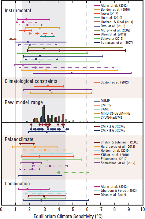
As a rough approximation, the long-term economic impacts vary as the square of the amount of global temperature increase (SCC, 2010; Kopp et al., 2012). As a result an ECS uncertainty of a factor of 4 leads to a factor of 16 uncertainty in long-term economic impacts, and is the largest single scientific uncertainty in estimating the impacts due to carbon emission scenarios (SCC, 2010). A factor of 2 reduction in ECS uncertainty would lead to a large reduction in the uncertainty of future climate change economic impacts, in the social cost of carbon, and in societal plans for future emissions reductions needed to limit climate change to an agreed upon maximum warming level. Reducing the uncertainty in climate sensitivity has been estimated to have an economic value of roughly $10 trillion U.S. dollars to global society at the Net Present Value discount rate of 3 percent used as the nominal value by the SCC 2010 (Cooke at al., 2014, 2016; Hope, 2015). The panel determined that narrowing the uncertainty in ECS, including quantified understanding of the feedback processes, should be one of the highest priorities of climate science.
Science Question and Application Goals
Question C-2. How can we reduce the uncertainty in the amount of future warming of Earth as a function of fossil fuel emissions, improve our ability to predict local and regional climate response to natural and anthropogenic forcings, and reduce the uncertainty in global climate sensitivity that drives uncertainty in future economic impacts and mitigation/adaptation strategies?
The following key objectives have been identified and are discussed in detail in the following sections:
- C-2a. Reduce uncertainty in low and high cloud feedback by a factor of 2 (Most Important).
- C-2b. Reduce uncertainty in water vapor feedback by a factor of 2 (Very Important).
- C-2c. Reduce uncertainty in temperature lapse rate feedback by a factor of 2 (Very Important).
- C-2d. Reduce uncertainty in carbon cycle feedback by a factor of 2 (Most Important).
- C-2e. Reduce uncertainty in snow/ice albedo feedback by a factor of 2 (Important).
- C-2f. Determine the decadal average in global heat storage to 0.1 W/m2 (67 percent confidence) and interannual variability to 0.2 W/m2 (67 percent confidence) (Very Important).
- C-2g (see also Question C-9). Quantify the contribution of the upper troposphere and stratosphere (UTS) to climate feedbacks and change by determining how changes in UTS composition and temperature affect radiative forcing with a 1-sigma uncertainty of 0.05 W/m2/decade (Very Important).
- C-2h (see also Question C-5). Reduce the IPCC AR5 total aerosol radiative forcing uncertainty by a factor of 2 (Most Important).
In order to address the science question, the quantitative linkage from process-level Earth system understanding to evaluation of feedbacks to ECS has to be considered. Reducing uncertainty in ECS has proven difficult since the first IPCC report (IPCC, 1990). What has been learned over the last 25 years of climate model and climate data analysis, however, are the sources of uncertainty in the estimation of ECS, and their relative magnitudes (Bony et al., 2006; Soden et al., 2008; IPCC, 2013). Considering these uncertainty sources, we choose as a realistic and critical goal the reduction of the IPCC AR5 uncertainty in ECS by a factor of 2. This type of goal has the advantage of not presupposing the actual value of ECS, but instead of reducing the uncertainty in its estimation. This in turn will greatly reduce uncertainty in societal decisions about the economic value of greenhouse gas emission reductions using current economic resources when compared to savings from reduced adaptation costs in the future.
Climate sensitivity can be quantified as the sum of individual climate feedbacks (Roe and Baker, 2007; Soden et al., 2008; IPCC 2013). Of these feedbacks, cloud feedbacks have been shown to be the largest
uncertainty in determining ECS in both observations and climate models (IPCC, 2013), particularly low cloud feedbacks. The process-level understanding involves the quantitative determination of how clouds affect circulation and vice versa (WCRP Grand Challenge). Uncertainty in the cloud feedback and the difficulty in estimating it arises partly from the fact that the spatial scales over which the processes have to be determined span several orders of magnitude (micrometers to kilometers; both horizontally and vertically; e.g., cloud microphysics to mesoscale convective complexes to spatially extensive cirrus shields). This poses an enormous challenge for observational strategies; however, spaceborne measurements offer the best coverage over the entire globe and represent the best opportunity to monitor all the global cloud regimes. The second largest uncertainty is the determination of the combined water vapor feedback and temperature lapse rate feedback. These two feedbacks have a strong negative correlation and are therefore normally considered as a combined feedback uncertainty even though uncertainty in each component can be much larger than the two in combination (IPCC, 2013). Indeed, the water vapor and cloud feedback processes together constitute the interplay between the elements of hydrologic cycle and energy. The lowest uncertainty in the climate sensitivity estimate is surface albedo feedback, which includes vegetation, soil characteristics, and snow/ice influences on the sunlight reflected off the planetary surface. Each of these physical climate system feedbacks is considered in this science question. Figure 9.9 shows a summary of the current understanding of uncertainty in climate feedbacks (from IPCC, 2013, Figure 9.23).
The most recent IPCC report included an extensive discussion of carbon cycle feedbacks and concluded that the uncertainty of these feedbacks, especially over land surfaces, can rival those of the physical climate system (IPCC WG1, 2013). The dominant feedback is the so-called concentration-carbon response
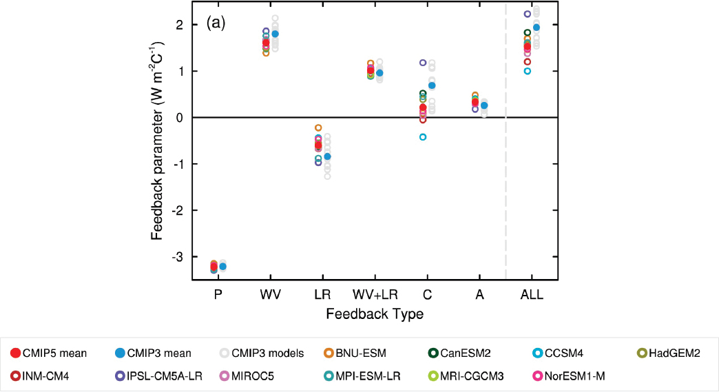
that describes the dependence of carbon storage in ocean and land reservoirs on the changing concentration of CO2 in the atmosphere (Gregory et al., 2009; IPCC, 2013). The Coupled Model Intercomparison Project Phase 5 (CMIP5) spread in the concentration-carbon response is greater for the land than for the ocean, and important processes are missing from many or all CMIP5 models, such as the role of nutrient cycles, permafrost, fire, and ecosystem acclimation to changing climate (IPCC, 2013). There is a second carbon cycle feedback that results from temperature change, but it is of much smaller magnitude and is similar in uncertainty to surface albedo feedback (IPCC, 2013). Carbon cycle processes and feedbacks are discussed briefly in the following section and treated in more detail by the Ecosystems Panel.
Similarly, aerosol forcing is considered separately in the following sections in terms of the processes governing their direct effect and their interactions with clouds, but here we note briefly two considerations of relevance for ECS. First, one of the key methods to estimate climate sensitivity from observations is to compare the time series of radiative forcing with that of temperature increase. In these types of comparisons the largest uncertainty is not the temperature record but is instead the poorly known levels of direct and indirect aerosol radiative forcing (IPCC, 2013). Reducing uncertainty in aerosol radiative forcing is therefore one method that can assist in reducing uncertainty in climate sensitivity. Second, while the largest feedback uncertainty as part of ECS is cloud feedback, the same clouds we would observe to examine cloud feedback could also be getting impacted by aerosols through the aerosol indirect effect. For both of these reasons the panel decided to include aerosol radiative forcing in this science question although the factors affecting these interactions are dealt with in a separate objective. The panel chose a similar factor of 2 reduction of uncertainty as the science goal.
Last, natural variability of the climate system provides the major “noise” against which anthropogenic climate change must be detected (Weatherhead et al., 1998; Leroy et al., 2008). This noise primarily increases the climate record length needed to clearly see anthropogenic climate signals, including those of climate feedbacks. Most of this noise is internal nonlinear variability of the ocean-atmosphere coupled system (IPCC, 2013). Transient variations in the climate system can arise due to temporary large loadings of stratospheric aerosols from explosive volcanic eruptions such as the 1982 El-Chichon and 1991 Mount Pinatubo eruptions (IPCC, 2013). Other natural factors that can potentially introduce variability, although with smaller amplitudes, include variations in solar irradiance and in naturally occurring tropospheric aerosols (e.g., dust). Knowledge of both natural variability and heat storage variations are required in order to understand and quantify the climate response to anthropogenic radiative forcing—namely, the “signal” above the internal/natural “noise.” Ascertaining natural variability is one prime reason for requiring sustained monitoring of the planet. Typically, variability of the climate system over century time scales is currently obtained from unforced climate model integrations, but long-term observations are required to verify and make these estimates robust.
The panel determined that achieving the objectives related to this science question will produce enormous benefit to both U.S. and global society. It will advance both the understanding of how humankind is forcing the climate system and thus climate responses for a given level of emissions against the backdrop of natural variations, as well as the ability to predict more accurately the future impact of those emissions on human society.
Society’s ability to see current climate forcing and climate change, as well as to predict future climate change, occurs through what can be thought of as three “fuzzy” lenses (Weatherhead et al., 2017). The first fuzzy lens is a result of the noise of natural variability. The second fuzzy lens is a result of the many limitations of our observing system. The third fuzzy lens is a result of limitations and uncertainties in the climate models used for understanding climate and for making climate predictions and projections. Aspects of each of these challenges are addressed in this critical science question.
Measurement Objectives and Approaches
The overarching science question, motivation, and goals lead to a set of quantified objectives involving the observation of physical climate system feedbacks, carbon cycle feedbacks, aerosol radiative forcing, and naturally driven variability of the climate system. The relative importance of each of these goals is based on uncertainties in recent major assessments such as the IPCC WG1 (2013). The largest of these uncertainties are (1) cloud feedback, (2) water vapor-plus-lapse rate feedback, (3) carbon cycle feedback, and (4) aerosol radiative forcing. The remaining quantified objectives are also important, but at a level significantly below these four.
As indicated in the “Introduction and Vision” section at the start of this chapter, solutions to climate science challenges require combined advances in climate process observations, climate modeling, and long-term monitoring observations. Figure 9.10 provides an example of how these elements work together. While the examples in the figure are most relevant to studies of clouds and aerosols, the overall approach is applicable to most climate science challenges.
Similar to the question of sea-level rise, high confidence in the understanding of climate system feedbacks and forcings requires both a measurement of the integrated effect of these long-term (interannual to decadal) changes in the radiation balance of Earth as well as measurement of the underlying physical variables driving the changes in energy balance. Achieving both measurements with consistent results provides a top-down and bottom-up independent verification of results and their uncertainties.
Long-term observations alone, however, are unlikely to be sufficient to improve the underlying process physics in climate models. Many of the uncertain modeling processes such as clouds and aerosols occur at short time and space scales (hours to days) and are often dominated by convection and large-scale dynamics rather than the radiation energetics that drives longer time scale global-mean forcings and feedbacks (Bony et al., 2015). Thus, additional observations specifically targeted at improving climate model processes are needed to enable improved accuracy of climate prediction (seasonal to decadal time scales) and climate projection (decade to century time scales). While modeling studies have enabled an understanding of the quantitative observing requirements for long-term climate feedbacks (Soden et al., 2008; Shea et al., 2017), equivalent observing requirements do not yet exist for cloud or aerosol process studies. This makes selection of new process study observations much more challenging. For example, what level of improvement is needed in measurements of cloud updrafts/downdrafts and mesoscale circulations; higher vertical resolution water vapor profiles; improved high vertical resolution boundary layer temperature, water vapor, and wind profiles; liquid and ice particle size distributions (cloud, rain, and snow); cloud condensation and ice nuclei concentrations; and improved vertical aerosol profiles? Which of these advances would be more important to understand and quantify cloud-climate interactions? While currently uncertain, it should be possible to develop quantitative objectives for process observations. In addition a range of new technologies have the potential to address some of these cloud and aerosol process observations. Table 9.3 provides some examples of potential improvements in cloud process measurements and potential technologies that might be used to address them.
Fortunately, cloud process models at very high spatial resolution of 10 meters to 1 km (Large Eddy Simulation to Cloud Resolving Model) can now run on domains of hundreds to thousands of kilometers, sizes large enough to capture cloud and larger scale dynamics as a system, and sizes that overlap the 30 km to 10 km grid resolution of global climate models. Nested global models that can run simulations on as fine a scale as ~1 km over limited areas of the globe are also under development (e.g., NOAA and NASA). This suggests that field experiments (e.g., EV-S selections) and their more complete data sets from surface, satellite, and aircraft might be used to more rigorously test cloud and aerosol process models on a global scale. It also suggests that high-resolution cloud model Observing System Simulation Experiments (OSSEs),
TABLE 9.3 Example Improved Cloud Process Measurements and Relevant Potential Space Technologies
| Example Cloud Process Measurement | Example Space Technology |
|---|---|
| Convective cloud updrafts and downdrafts | Doppler radar |
| High vertical resolution accurate water vapor profiles (~100 m, <5% accuracy) | Differential absorption (DIAL) lidar, water vapor absorption line microwave radio occultation |
| High vertical resolution boundary layer profiles of temperature, water vapor, wind speed/direction | Surface scatterometer winds, wind lidar, DIAL lidar, water vapor radio occultation, temperature lidar using molecular oxygen density |
| High time resolution (e.g., 15-minute sampling) | Smallsat constellations, geostationary satellites |
| High-accuracy precipitation and drop size distribution | Multiwavelength doppler radar, multifield of view lidar |
| Multilayer cloud vertical profiles | Radar, lidar |
| Thin cirrus vertical distribution, optical properties | High spectral resolution lidar |
| Surface pressure | Molecular oxygen lidar, Molecular oxygen A-band, numerical weather prediction (NWP) assimilation |
| Large-scale vertical velocities (50 km and larger) | No current candidate |
including global-mesoscale-nested models, might ultimately be capable of more rigorous definition of field experiment and satellite observations needed to test key uncertainties in the process models. While field experiment observations can provide a more complete set of relevant process variables, satellite observations can provide tests on global scales with large statistical sampling. This dichotomy suggests that field experiments and high-resolution cloud models as well as emerging high-resolution global models with nesting capabilities (~1 km resolution over the continental United States) that maintain a physical consistency between large-scale and mesoscale processes might be gainfully used to determine observing system requirements for later global observations from space. In parallel with the field experiments NASA technology programs can be maturing the next generation measurement capabilities. Last, as process models reach higher resolutions and begin to resolve cloud physical processes, existing observations such as from the Afternoon Constellation (A-Train) can be used in new ways to constrain the advancing model capabilities.
Following the earlier discussion, the Climate Panel SATM related to climate sensitivity is focused primarily on long-term observations required to constrain uncertainty in Earth’s forcings and feedbacks. From an observations standpoint, the ECS quantification is a less difficult proposition than the comprehensive approach centered on the quantification of each relevant process. As examples of the difficulty, the processes shaping low and high clouds are significantly different, involving various facets of the tropospheric large-scale circulation and convection. Also, precipitation becomes a key element in the understanding of cloud feedbacks, since it affects the lifetime and energy exchanges.
There is less discussion here of the observations that might enable improved process models because of the current difficulty in relating those observations to quantified objectives, and the difficulty of prioritizing which observations are more critical than others or which ones will yield greater dividend earlier. This should not be interpreted as any lack of importance of process observations, nor does it imply that important process-level observations of some relevant aspects of feedbacks are not occurring or are not possible. (For example, cloud radar observations have pointed to an important feedback involving drizzle in clouds that does not appear to be simulated by climate models or well understood.) Instead, the preceding statement should be interpreted as an uncertain balance between the value of field experiments, satellites, and the key variables to measure for each. It is expected that some of the short time scale weather and hydrology science questions will be relevant for process studies of forcings and feedbacks, as will some of
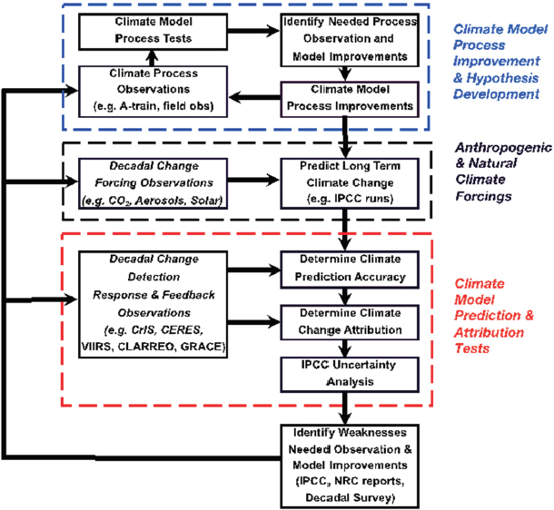
the observations required for long-term observations of forcings and feedbacks, in addition to the existing satellite process observations such as the 10-year A-Train record. We also note that the World Climate Research Programme (WCRP) Grand Challenge on climate sensitivity is focused on several cloud and general circulation modeling studies, along with studies of past observations to move toward improved cloud process models.8 Ultimately, development and testing of improved cloud and aerosol process models will require advanced short time scale process observations (say, from weather to seasonal time scales), while climate model projection accuracy using the new processes must be verified using sufficiently accurate and complete long-term decadal observations, as shown in Figure 9.10.
A high-level summary of the quantified science objectives and potential measurement approaches is given in this section. Further details can be found in the Climate Panel SATM (see Appendix B).
Objective C-2a. Reduce uncertainty in low and high cloud feedback by a factor of 2 (Most Important).
The largest uncertainty in ECS is caused by low cloud feedback (IPCC, 2013). Climate models vary from negative to positive feedback for low clouds. Studies to separate feedbacks using radiative kernels (Soden et al., 2008; IPCC, 2013) suggest that multidecadal records of shortwave cloud radiative effect (SWCRE) can be used to determine cloud feedback. A similar method is used in analysis of climate model simulations. Verification that the SWCRE is caused by the correct cloud property (cloud fraction, optical
___________________
8 See https://www.wcrp-climate.org/gc-clouds-circulation-activities/gc4-clouds-initiatives.
depth, phase, particle size) requires observations by CALIPSO-like lidar (cloud fraction, phase) and Visible Infrared Imaging Radiometer Suite (VIIRS)-like global imager (cloud fraction, optical depth, phase, and particle size). Progress has been made in unscrambling cloud feedbacks by cloud property (Zelinka et al., 2012, 2017). These studies suggest that the largest feedbacks occur from changes in cloud fraction, followed by cloud height, and finally cloud optical depth. The optical depth feedback in turn is dominated by changing cloud droplet phase from larger ice crystals to smaller water droplets in high southern latitudes (Zelinka et al., 2012). As a result even cloud particle phase is important to consider as a cloud feedback measurement. To date, the satellite record of SWCRE and cloud properties has lacked sufficient climate record length and accuracy to directly observe low cloud feedback at the required uncertainty level (Dessler, 2010, 2013; IPCC, 2013). The suggested measurement approach to resolve this issue is to continue the climate record of global radiation budget observations by Cloud-Earth Radiant Energy System (CERES)/Radiation Budget Instrument (RBI) and VIIRS to achieve the long record length, but augmented for greater accuracy by intercalibrating CERES/RBI and VIIRS radiometers to a reference SI traceable transfer spectrometer at the required 0.15 percent (k = 1) accuracy level as proposed in the 2007 Decadal Survey Climate Absolute Radiance and Refractivity Observatory (CLARREO) mission (NRC, 2007; Wielicki et al., 2013; Shea et al., 2017).
High cloud feedback is large and positive in all major climate models and results primarily from a change in high cloud height, and therefore in a change between high cloud temperature and surface temperature. The Fixed Anvil Temperature (FAT) hypothesis affords an explanation of the basic large-scale physics of this feedback in the tropics (Hartmann and Larson, 2002). The key radiative fluxes for high cloud feedback are longwave fluxes, while the key cloud physical properties are cloud amount, cloud height, and cloud top temperature. It is noted though that these governing properties are themselves affected by atmospheric dynamics and microphysical (mixed-phase and solid ice) processes. Unfortunately, sufficiently accurate decadal time scale cloud height, temperature, and flux observations from space have not yet been available to directly observe this feedback (IPCC, 2013). For ice clouds, the challenge is even more daunting than for water clouds owing to serious gaps in knowledge of dynamics and microphysics. There are two suggested ways to provide the required accuracy in the observations to verify high cloud feedback: (1) long-term space-based atmospheric lidar similar to at least CALIPSO capability for more accurate cloud height; and (2) much higher accuracy (0.03 k = 1) SI traceable infrared observations from visible/infrared imagers similar to VIIRS, and higher accuracy broadband radiation measurements. One method to achieve this higher accuracy using the operational NOAA VIIRS and NASA CERES/RBI sensors is to intercalibrate each against a reference SI traceable infrared transfer spectrometer at this accuracy level as proposed in the 2007 Decadal Survey CLARREO mission (NRC, 2007; Wielicki et al., 2013; Shea et al., 2017). The requirement for a multidecade record is determined by natural variability of tropical and global average cloud amount, height, and radiative fluxes.
Objective C-2b. Reduce uncertainty in water vapor feedback by a factor of 2 (Very Important).
While cloud feedback is by far the largest uncertainty in ECS, the combination of water vapor feedback and temperature lapse rate feedback (Objective C-2c) are the second largest uncertainties in the physical climate system sensitivity. Current uncertainties are determined from climate model agreement, the Clausius Claperyon relationship of specific humidity increase with temperature at constant relative humidity (7 percent/K) and observations of column water vapor decadal changes (IPCC, 2013). Further observational constraint of water vapor feedback requires decadal time series of temperature profiles and water vapor profiles at higher accuracy than current satellite or surface instruments provide (Xu et al., 2017). In addition, the far-infrared spectrum (longwave radiation at wavelengths beyond 15 micron) has not been observed
spectrally, yet this is half of the thermal infrared radiation and the dominant portion of the water vapor greenhouse effect and the dominant source of water vapor feedback. The far-infrared has been observed by broadband radiation instruments such as CERES but only for the integrated longwave radiation across all infrared wavelengths. As a result, there is a marginal observational constraint on changing temperature profile, water vapor profile (especially upper troposphere), and far-infrared spectral radiation trends. One method to achieve such an advance is to utilize decadal trends from the current NOAA Cross-track Infrared Sounder (CrIS) mid-infrared sounder and CERES/RBI broadband radiometer calibrated against a higher accuracy SI traceable standard at the 0.03K (k = 1) accuracy requirement indicated for anthropogenic climate trends by recent studies (Xu et al., 2017). A high-accuracy infrared reference spectrometer including the far-infrared spectrum was proposed by the 2007 Decadal Survey CLARREO mission (NRC, 2007). Global Navigation Satellite System Radio Occultation (GNSS RO) systems such as Constellation Observing System for Meteorology, Ionosphere, and Climate (COSMIC) and COSMIC-2 can provide high-accuracy trends for vertical temperature profiles between 5 and 20 km altitude, but only lower level water vapor profiles. Accuracy of commercial radio occultation systems has yet to be demonstrated. High-accuracy, high vertical resolution water vapor profiles have been proposed using radio occultation signals at new wavelengths in varying strength microwave water vapor absorption lines, and by differential absorption lidar.
Objective C-2c. Reduce uncertainty in temperature lapse rate feedback by a factor of 2 (Very Important).
The logic for this objective is similar to that in Objective C-2b, but without the requirement of water vapor profile or far-infrared spectra observations. Meeting this objective would therefore rely on a combination of CrIS spectrometer observations with GNSS RO systems such as COSMIC and COSMIC-2, or with CrIS combined with intercalibration to a high accuracy (0.03K, k = 1) SI traceable infrared spectrometer such as the 2007 Decadal Survey CLARREO mission (NRC, 2017).
Objective C-2d. Reduce uncertainty in carbon cycle feedback by a factor of 2 (Most Important).
The uncertainty on the carbon cycle is of comparable magnitude to the uncertainty arising from physical climate processes (Gregory et al., 2009; IPCC WG1, 2013), and the panel recognizes the critical and obvious need for measurements to reduce this uncertainty with the designation of Objective C-2d as Most Important. Due to the complexity of measuring and predicting carbon cycle processes, we devote a separate section of this chapter to the topic “C-3: Carbon Cycle, Including Carbon Dioxide and Methane.” Note that the Question C-3 objectives are defined with granularity required to derive mission requirements, and consequently no individual C-3 objective is sufficiently broad to receive a rating of Most Important by the Climate Panel. Carbon cycle feedbacks are also treated in Chapter 8.
Objective C-2e. Reduce uncertainty in snow and ice albedo feedback by a factor of 2 (Important).
Surface albedo is the smallest uncertainty feedback, both because of its smaller magnitude and because of the fact that seasonal cycles of snow and ice and sea-ice albedo change have been shown to be a very accurate proxy for the long-term feedback of snow and ice albedo (IPCC, 2013). There are no new observational requirements beyond the operational NOAA VIIRS instrument and a longer accurate climate record to achieve this objective. This observation does not require intercalibration of VIIRS to the high accuracy of the CLARREO reference spectrometer mentioned for cloud feedback or temperature and water vapor feedback to achieve.
Objective C-2f. Determine the decadal average in global heat storage to within 0.1 W/m2 (67 percent confidence), and interannual variability to 0.2 W/m2 (67 percent confidence) (Very Important).
This objective overlaps with Objective C-1b at decade and longer time scales. But it adds an interannual component to identify shorter term natural variability of ocean heat storage that Argo sampling cannot achieve. This interannual capability is currently provided by combining Total Solar Irradiance (TSI) observations from Solar Radiation and Climate Experiment (SORCE) and broadband radiation observations from CERES (Von Schuckmann et al., 2016; Hansen et al., 2017). While net radiation alone cannot determine climate sensitivity (due to uncertainty in ocean vertical mixing rates), it does provide a very useful constraint when combined with other observations such as reduced uncertainty aerosol forcing and improved cloud feedback observations.
The panel also notes the importance of monitoring the interannual and decadal variations of the natural radiative forcings of volcanic eruption aerosols and of Total/Spectral Solar Irradiance variability (Hansen et al., 2005; IPCC WG1, 2013; NRC, 2013, 2015) to an accuracy of 0.05 W/m2 per decade. In the context of naturally occurring aerosols and their plausible interactions with clouds, there will be a need to also monitor the influence of dust emissions from surfaces globally, which can vary on a year-by-year and decadal basis (Prospero et al., 2002; Ginoux et al., 2012; IPCC WG1, 2013). These measurements are important for a wholesome determination of the ECS.
Connections to Other Panels and Integrating Themes
For a given forcing of the system, feedbacks determine the amplitude of the climate system response. In this sense climate forcings and feedbacks link to the Hydrology, Weather and Air Quality, and Ecosystems Panels through the long-term changes in all of these Earth systems. In the same sense climate feedbacks also link closely to the Water and Energy Integrating Theme, the Water Cycle Integrating Theme, and the Carbon Cycle Integrating Theme, as well as the Natural Hazards and Extreme Events Integrating Theme. In some cases the linkage is obvious, as for the carbon cycle climate feedback objective, which overlaps with the Ecosystems Panel as well as the Carbon Cycle Integrating Theme. Another major example is the linkage of the energy cycle and the water cycle through Earth’s energy system. Changes in climate forcings and feedbacks modify Earth’s energy cycle, which in turn modify the latent heat and precipitation water cycle. Latitudinal changes in the energetics of forcings and feedbacks (e.g., polar amplification) can also drive circulation changes that then lead to changes in the mean hydrologic cycle as well as the frequency of extremes.
C-3: Carbon Cycle, Including Carbon Dioxide and Methane
Motivation
Carbon dioxide (CO2) is the most important anthropogenic greenhouse gas (GHG). The dry air mole fraction of CO2 has risen from a preindustrial value of ~280 parts per million (ppm) to a contemporary value that exceeded 400 ppm in 2016 (Figure 9.11). Early in the 20th century the rise in atmospheric CO2 was driven by the clearing of forests for agriculture. Over the past 70 years this rise has been driven by increasing combustion of fossil fuels (IPCC, 2013).
Methane (CH4) is the second most important GHG emitted by human society. CH4 has risen from a preindustrial level of 700 ppb to a contemporary value of more than 1800 ppb (Figure 9.11). The radiative forcing (RF) of climate driven by rising CH4 is about 30 percent of the RF caused by rising CO2. Weighted

by mass, the release of a pulse of CH4 has a global warming potential that is 84 times that of CO2 over a two-decade time horizon, and 28 times CO2 over a century. These estimates of global warming potential (GWP) of CH4 rise to 86 and 34 for the two time horizons, respectively, when allowance is made for carbon cycle feedback (IPCC, 2013). Anthropogenic emissions of CH4 occur for many sectors of a modern economy, including fossil fuel extraction and use, ruminants (i.e., mammals such as cattle and sheep that acquire nutrients from food via fermentation prior to digestion), agriculture (particularly crops that prefer wet anaerobic conditions such as rice), landfills, and sewage treatment, whereas natural sources are dominated by emissions from tropical and northern wetlands (i.e., seasonally or perennially flooded regions), biomass burning, termites, lakes, and geological sources.
There presently exists considerable uncertainty in the recent carbon budget and in projections of how atmospheric CO2 will respond to climate change (Ciais et al., 2013). Recent studies have reported increasing terrestrial sinks due to CO2 fertilization (Zhu et al., 2016; Los et al., 2013; Schimel et al., 2015; Keenan et al., 2016). Meanwhile, other studies covering diverse regional ecosystems suggest reduced carbon uptake due to droughts and other extreme events (e.g., Ma et al., 2012; Reichstein et al., 2013; Zhou et al.,
2014; Brienen et al., 2015). Friedlingstein et al. (2014) evaluated simulations of end of century CO2 from 11 atmospheric, oceanic general circulation models with an interactive carbon cycle. Variations of CO2 in 2100 ranged from 795 to 1145 ppm for the same fossil fuel emission scenario, with differences mainly attributable to the response of the land carbon cycle. Booth et al. (2012) found even larger differences (a range of 461 ppm) using a single coupled climate-carbon cycle model and perturbing key land carbon cycle parameters over ranges consistent with their uncertainties. Using a price of $13/ton of atmospheric CO2, 400 ppm of CO2 has a present-day economic value of $40 trillion.9
Projections of future atmospheric CH4 are also highly uncertain. The scenarios for future GHG abundance developed for IPCC (2013), termed Representative Concentration Pathways (RCPs), project that CH4 could be as high as 3750 ppb (RCP 8.5) or as low as 1250 ppb (RCP 2.6) in year 2100 (Riahi et al., 2011; van Vuuren et al., 2011). This uncertainty is driven by disparate assumptions regarding whether, and how effectively, human emission of CH4 will be managed and curtailed. Furthermore, the mechanisms driving recent methane trends are not well understood. The observed stabilization of methane levels between 1996-2006 and renewed increase after 2006 may be attributable to a slowdown in fossil fuel emissions followed by an increase in biogenic emissions such as from tropical wetlands or increased agricultural sources (Kirschke et al., 2013; Nisbet et al., 2016; Schaefer et al., 2016). An alternative hypothesis to explain recent increases in CH4 is a decrease in concentration of the hydroxyl radical, the largest methane sink (Rigby et al., 2017; Turner et al., 2017). Schwietzke et al. (2016) used methane isotope data to show that fossil sources of methane are higher than previously estimated and that there is no significant trend in fossil sources, but their analysis could not distinguish between emissions from fossil fuel industrial activity versus natural geologic seepage. Conversely, Wolf et al. (2017) suggest that changes in livestock management and practices may account for 50 to 75 percent of the recent rise in atmospheric CH4. This lack of consensus reflects the current state of knowledge, and additional measurements are needed that can differentiate among the various hypotheses.
Projections for CH4 are complicated by possible alteration of wetland sources due to climate-change induced changes in the hydrologic cycle (i.e., floods and droughts), release of possible large amounts of CH4 upon thawing of the Arctic permafrost (Schuur et al., 2015), and leakage from the extraction or transportation of natural gas (Karion et al., 2013). To date, the release of CH4 from the thawing of permafrost is small on a global scale (Walter Anthony et al., 2016).
Science Question and Application Goals
Question C-3. How large are the variations in the global carbon cycle and what are the associated climate and ecosystem impacts in the context of past and projected anthropogenic carbon emissions?
To advance understanding of the global carbon cycle (i.e., CO2 and CH4), the panel has suggested the following objectives:
- C-3a. Quantify CO2 fluxes at spatial scales of 100-500 km and monthly temporal resolution with uncertainty <25 percent to enable regional-scale process attribution explaining year-to-year variability by net uptake of carbon by terrestrial ecosystems (i.e., determine how much carbon uptake results from processes such as CO2 and nitrogen fertilization, forest regrowth, and changing ecosystem demography) (Very Important).
___________________
9 See Climate Policy Initiative, “California Carbon Dashboard,” http://calcarbondash.org.
- C-3b. Reliably detect and quantify emissions from large sources of CO2 and CH4, including from urban areas, from known point sources such as power plants, and from previously unknown or transient sources such as CH4 leaks from oil and gas operations (Important).
- C-3c. Provide early warning of carbon loss from large and vulnerable reservoirs such as tropical forests and permafrost (Important).
- C-3d. Provide regional-scale process attribution for carbon uptake by ocean to within 25 percent (especially in coastal regions and the Southern Ocean) (Important).
- C-3e. Quantify CH4 fluxes from wetlands at spatial scales of 300 km × 300 km and monthly temporal resolution with uncertainty better than 3 mg CH4 m–2 day–1 in order to establish predictive process-based understanding of dependence on environmental drivers such as temperature, carbon availability, and inundation (Important).
- C-3f. Improve atmospheric transport for data assimilation/inverse modeling (Important).
- C-3g. Quantify the tropospheric oxidizing capacity of OH, critical for air quality and dominant sink for CH4 and other GHGs (Important).
Quantification of greenhouse gas (GHG) fluxes at continental, regional, and local scales is needed (1) to assess the efficacy of policies included in international climate agreements, and (2) to understand the processes controlling the natural components of the carbon cycle, which in turn will lead to models with better predictive abilities under changing climate conditions. Satellite observations of CO2, such as those provided by the Orbiting Carbon Observatory-2 (OCO-2) and Greenhouse Gas Observing Satellite (GOSAT) and from potential future missions such as GOSAT-2 and the recently announced Geostationary Carbon Cycle Observatory (GeoCARB), have the potential to play a pivotal role, if systematic errors are identified and remedied.
The panel also identified numerous other Important goals (see Appendix B) focused on quantification of CH4 fluxes from wetlands at high spatial resolution as well as the development of a reliable predictive capability for future change in this source, quantification of CO2 and CH4 emissions from urban areas and point sources, early warning of the loss of carbon from vulnerable ecosystems, as well as understanding how climate change will alter the oxidative capacity of the troposphere (i.e., how tropospheric mean [OH] will respond to global warming). Large contemporary uncertainties in all these areas limit our confidence in the representation of carbon cycle feedbacks within global models (IPCC, 2013).
Measurement Objectives and Approaches
The predominant approach for satellite-borne CO2 and CH4 sensors such as OCO-2, GOSAT, and the Tropospheric Monitoring Instrument (TROPOMI) measures absorption of reflected near-infrared light. Passive sensors measure reflected sunlight, while proposed active sensors such as the Active Sensing of CO2 Emissions over Nights, Days, and Seasons (ASCENDS) mission recommended by the ESAS 2007 and the planned French-German Methane Remote Sensing Lidar Mission (MERLIN) would employ lasers. Passive satellite observations of XCO2 are unevenly distributed across the globe and may have aerosol, thin-cloud, albedo, surface-type, solar zenith angle, or other coherent space- and time- dependent biases. Passive sensors are limited to sunlit conditions and so do not provide data for nighttime or for high-latitude winter scenes, limiting sensitivity to possible increasing emissions from vulnerable Arctic reservoirs (see Objective C-3c). Retrievals from passive sensors are limited to cloud-free conditions and hence have a fair-weather bias. Active sensors are uniquely capable of providing nighttime data and are arguably less susceptible to biases associated with aerosols and clouds, but active sensors have increased complexity and power requirements and provide limited spectral information. The recently announced GeoCARB mission is an
OCO-2-like passive sensor in a geostationary orbit that will provide dense data over temperate and tropical North and South America with additional spectral channels for CH4 and CO. The dense sampling will be especially useful for monitoring urban emissions and emissions from large point sources (C-3b). GeoCARB is expected to provide new constraints on estimates of fluxes from tropical wetlands and insights into how wetland fluxes respond to changes in environmental drivers such as temperature and inundation (C-3e).
Both passive and active techniques provide a column-integrated measurement, with limited information about the structure of the vertical profile. The signal of regional sources/sinks is typically diluted in the full column to 20 to 30 percent of its strength in the boundary layer. Day-to-day variability in XCO2 is strongly influenced by synoptic weather patterns, obscuring signatures of surface fluxes. Kulawik et al. (2016) have recently developed a method for separately estimating lower and upper tropospheric partial column CO2 with GOSAT data, and comparisons with aircraft measurements demonstrate the potential for this approach. Midinfrared sensors are already in orbit on weather satellites and can potentially provide additional information about midtropospheric CO2 and CH4 abundance. However, midinfrared sensors have little to no sensitivity to the surface layer, where signatures of emission and uptake are strongest. The combination of near- and midinfrared spectral information should enable some separation of boundary layer and midtropospheric signals. However, in practice, this requires extremely careful characterization of the sensors, and a consistent retrieval strategy. Future satellite sensors may employ a variety of combined approaches, including active/passive, geostationary versus low-Earth orbit, high spatiotemporal resolution over targeted areas versus broad-area mapping, and combined near-IR/mid-IR spectroscopy.
For flux estimation, systematic biases in retrievals are more problematic than random errors and can be reliably detected and quantified only if sufficiently informative ground truth data are available. The OCO-2 and GOSAT science teams have worked diligently to identify and mitigate systematic biases in retrievals (Wunch et al., 2011a; Lindqvist et al., 2015; Wunch et al., 2016; Crisp et al., 2017; Eldering et al., 2017), but even small biases in XCO2 can cause significant errors in estimated fluxes. Quantification of subtle signals resulting from changes in emissions and from climate-induced biological flux anomalies will require the ability to sense gradients and detect trends with long-term stability (i.e., over periods of months to years) of ~0.2 ppm in XCO2 maintained over many years (Wofsy and Harris, 2002; NRC, 2010). Measurement requirements to detect important flux signatures at local to continental scales are discussed in a report on the notional CarbonSat mission that was proposed to ESA and are consistent with the requirements in the SATM (ESA, 2015). The systematic error goal for CarbonSat is 0.2 ppm for CO2, a factor of 2 or more better than what has been demonstrated so far for OCO-2. The CarbonSat systematic error goal for CH4 is 2.5 ppb, compared to 2 percent (or roughly 40 ppb) for the planned TROPOMI sensor.
The current strategy for evaluating OCO-2 retrievals relies on the Total Carbon Column Observing Network (TCCON). TCCON uses ground-based spectrometers similar to OCO-2 and GOSAT but with higher spectral resolution. TCCON retrievals have been linked to the World Meteorological Organization CO2 and CH4 scales via infrequent overflights by research aircraft (Wunch et al., 2010; Messerschmidt et al., 2011). The aircraft profiles typically have a maximum altitude between 10 and 12 km and so the stratospheric contribution to the column has to be approximated. Starting in 2012 the balloon-borne AirCore sampling system (Karion et al., 2010) has been routinely deployed over certain TCCON sites and provides profiles of calibrated in situ CO2 and CH4 up to ~28 km. Wunch et al. (2015) estimate that systematic biases of 0.2 percent for XCO2 (0.8 ppm) and 0.4 percent (7 ppb) for XCH4 could exist with the TCCON network. Site-to-site comparability of XCO2 of 0.2-0.56 ppm and XCH4 at the level of 1.5- 4.6 ppb for CH4 has recently been demonstrated across four TCCON sites in the United States during a 5-week campaign using a pair of mobile spectrometers (Hedelius et al., 2017). Comparisons between TCCON and OCO-2 show a median difference of less than 0.5 with root-mean-square differences typically less than 1.5 ppm (Wunch et al., 2016).
Strategic investments in infrastructure for additional ground truth are needed that will enable identification and mitigation of remaining systematic biases and that will serve a variety of emerging measurement concepts. Ongoing evaluation will be necessary, since satellite sensors may drift or degrade over time, and any seasonally or spatially varying retrieval biases would not be revealed by limited validation experiments. Frequent vertical profile data covering a range of latitudes and conditions have been crucial for correcting biases in satellite ozone retrievals and enabling trend detection across missions. Profile data are equally necessary for XCO2 and XCH4, but are currently limited. NOAA performs biweekly to monthly aircraft sampling at 14 sites over North America and from the island of Raratonga up to altitudes of ~8 km, and intensive campaigns such as the Atmospheric Carbon and Transport—America (ACT-America) and the Atmospheric Tomography (ATom) experiments also provide vertically resolved validation data. Internationally, the National Institute for Environmental Studies of Japan has implemented a commercial aircraft CO2 sampling program (Machida et al., 2008), and the European In-service Aircraft for a Global Observing System (IAGOS) program will begin measuring CO2 and CH4 from commercial aircraft later this year. Expanded commercial aircraft sampling is a promising mechanism for obtaining a large volume of crucial validation data needed to realize the potential of current and future greenhouse gas emissions and to establish continuity across missions. Ongoing site-to-site comparisons with portable spectrometers are needed to establish and track comparability across the global TCCON network, while continued routine AirCore overflights at key sites are needed to maintain the link between TCCON and the in situ network.
In addition to their value for evaluating satellite retrievals, ground-based, airborne, and shipboard in situ data have independent value for estimating carbon fluxes and are necessary for resolving flux signals that are too subtle for satellites to detect, such as gradients and trends resulting from ocean fluxes in critical regions such as coastal fluxes and Southern Ocean fluxes (see Objective C-3d; see also Objective C-4a for more discussion of air-sea fluxes of CO and CH4). The main advantage of satellite sensors is their global vantage point. GOSAT and OCO-2 are providing new information in regions where other types of atmospheric data are sparse, and they provide information about spatial patterns of flux that will drive improvements in process-based models. Conversely, the usefulness of point measurements is limited by sparseness in space and time. Consequently, the best flux estimates will come from a combination of remote-sensing and in situ measurements from a variety of platforms.
Connections to Other Panels and Integrating Themes
Ecosystems Panel
Carbon cycle-climate feedbacks are also addressed by the Ecosystems Panel, and discussion of measurements such as vegetation indices, biomass, and solar-induced fluorescence are described in Chapter 8. This panel has focused on carbon-climate questions related to predicting future radiative forcing, whereas the Ecosystems Panel also considers how changing atmospheric CO2 and future climate may affect ecosystems (CO2 fertilization, ocean acidification, changing ecosystem demography in response to changing climate).
Weather and Air Quality Panel
This panel is focusing on the co-benefit, for air quality, of slowing down or stopping the rate of growth of methane. Methane is a precursor of tropospheric ozone, and increases since preindustrial time have played an important role in driving a rise of ozone throughout the global troposphere. While the primary societal benefit for limiting the growth of methane will be to reduce the rate of global warming, the air quality co-benefit has been noted in many papers (e.g., Fiore et al., 2002).
The extent to which surface fluxes of CO2 and CH4 can be inferred from measurements of atmospheric abundance depends on the fidelity of atmospheric transport models used in data-assimilation systems. Question C-3 addresses this need, but the measurement requirements are not well defined. This is an important linkage with the Weather Panel, and it is important to note that certain considerations that are critical for trace constituent transport (e.g., dry air mass conservation) are not typically taken into account for weather prediction. Measurements and model improvements that lead to improved simulation of atmospheric transport would have far-reaching benefits across atmospheric science, including for air quality and general atmospheric composition questions.
C-4: Atmosphere-Ocean Flux Quantification
Motivation
A key component in the dynamics of the Earth system is the interaction between the atmosphere and the ocean. This interaction, which occurs through transfers (or fluxes) of heat, momentum, and mass (e.g., water vapor, sea spray, CO2, and DMS), provides feedbacks through the boundary layers of the atmosphere and oceans to modulate ocean and atmospheric circulations, the ocean heat content, the global water and energy cycles, the concentration of CO2 in the atmosphere by sequestration in the ocean and subsequent evasion, and the modulation and production of low-level clouds through oceanic aerosol production of cloud condensation nuclei. These interactions occur across a wide range of time and space scales, from the relatively fast weather exchanges at storm scales to centennial global variability. Thus, measuring these fluxes is imperative to understanding the processes leading to variability of the Earth system. For example, understanding how much heat and carbon the ocean absorbs is vital to understanding sea-level rise and to predicting how much, how fast, and where the atmospheric temperature will change, as the ocean stores more than 90 percent of the excess heat that has been added to the climate system over recent decades (e.g., Cheng et al., 2017) and roughly 30 percent of the excess carbon (Mikaloff Fletcher et al., 2006; Le Quéré et al., 2010).
It is also essential to understand the partitioning of the global energy imbalances between the atmosphere and ocean, as this is critical to defining the climate response to anthropogenic forcings. Currently, the surface energy and water budgets do not close, to a large extent due to imbalances between the radiative and turbulent heat fluxes and the evaporation and precipitation across the ocean surface (e.g., Stephens et al., 2012; L’Ecuyer et al., 2015). As can be seen in Figure 9.12, the evaporation from the ocean to the atmosphere represents the single largest term in the global water budget, and current estimates of the total magnitude require significant adjustment to bring balance to the budget. Other components of the water budget (precipitation in particular) are of roughly the same magnitude and uncertainty, but given the connection of the evaporation to the energy cycle, bringing balance to both appears to require larger adjustments to ocean evaporation than precipitation (L’Ecuyer et al., 2015; Rodell et al., 2015). The warming of the upper ocean tends to be reflected in trends of increasing ocean evaporation (i.e., water vapor flux) and precipitation in the hydrologic cycle, all of which can be and have been observed by evaluating the upper ocean salinity over time (e.g., Durack and Wijffels, 2010). These variations in the global hydrologic cycle are not restricted to over-ocean locations but affect precipitation patterns across land surfaces as well. The movement of water from the ocean to the atmosphere, where it then becomes available as precipitation to fall over both the ocean and land surfaces, is vital to life on land. However, our ability to predict the timing and magnitude of these variations is due in part to the uncertainties in the current global air-sea flux products, which prevent them from being used to quantify the trends in either the heat or the moisture budget (IPCC, 2013), as uncertainties are on the order of 10 to 20 percent (e.g., Gulev et al., 2011).
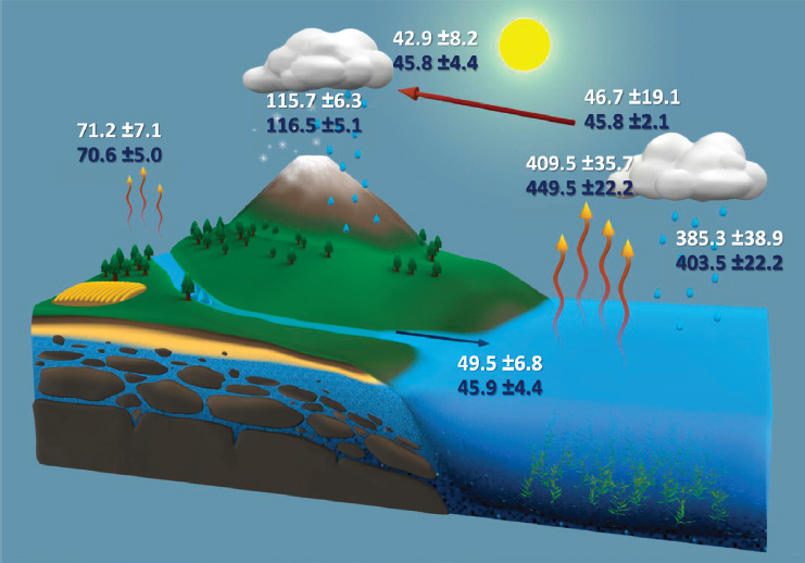
The exchange of momentum in addition to heat and moisture through the ocean surface drives the ocean circulation, upper ocean mixing, and surface wave fields, and provides a drag on the atmosphere. The overturning circulation in high latitudes, which helps drive the larger scale thermohaline circulation, is highly dependent on air-sea fluxes. In addition, the momentum flux to the ocean and resulting breaking wave fields provide a significant fraction of the aerosols that form the basis in the lower atmosphere for cloud formation, particularly in remote areas of the ocean. Uncertainties in how sea spray is generated by breaking waves limit our understanding of the transfer of heat and momentum between the ocean (e.g., Mueller and Veron, 2014), as well as limiting our ability to accurately reproduce the feedbacks between the upper ocean surface, aerosols, and low-level clouds. A number of analyses using combinations of satellite-based data sets, in situ observations, and reanalysis products have shown varying changes in wind-stress trends at decadal to centennial time scales; however, the variability between these analyses is large, and thus our knowledge of the actual change in time of these fields is low (IPCC, 2013). Increases in wind-stress fields from the tropical Pacific and Southern Ocean regions have been noted (e.g., Merrifield et al., 2012; Swart and Fyfe, 2012), but variations due to interannual variability are large and poorly understood (IPCC, 2013), and are complicated by Sun-synchronous observations of a variable with substantial diurnal and semidiurnal variability (Wentz et al., 2017).
Similarly, the scientific community lacks a robust understanding of how to estimate the exchange of CO2 between the ocean and atmosphere given the few variables that can be measured and the significant uncertainties surrounding other key variables (e.g., wind speed and thermal stratification) that are needed to calculate this exchange. On centennial time scales, basic scientific principles dictate that the ocean CO2 amount will equilibrate with atmosphere CO2, but an open question remains as to the rate at which this ocean uptake will occur, and our understanding of some key processes that control the carbon distributions in the ocean is still limited. Due to the dearth of observations, it is still unclear whether the rate at which the ocean is taking up CO2 is changing, with some analyses indicating a decline in the ocean uptake rate of total CO2 (Le Quéré et al., 2007; Schuster and Watson, 2007; McKinley et al., 2011), and
others finding a lack of evidence for a decrease (e.g., Knorr, 2009; Gloor et al., 2010; Sarmiento et al., 2010). Future estimates are even more uncertain, with recent studies suggesting that the Southern Ocean might increase carbon uptake, possibly enough to change the global net uptake to increasing rather than decreasing (Doney, 2010). Current observation-based estimates of the climate response of the global air-sea CO2 flux do not include feedbacks from ocean warming and circulation variability, which could make a difference of 20 to 30 percent in the ocean response (IPCC, 2013). Given that the ocean stores roughly 50 times as much inorganic carbon as the atmosphere (Sabine et al., 2004c), variations in the exchanges between the ocean and atmosphere can affect the atmospheric concentration of CO2, while also impacting the rate and magnitude of the ocean acidification (Doney et al., 2009).
Therefore, satellite observations of these air-sea fluxes are a crucial component of the measurement system given that in situ measurements are costly and difficult to implement, and we are currently unlikely to attain the needed temporal and spatial resolution and global coverage through these measurements. However, as many of the questions raised here require process-level understanding, investment in in situ measurements should also be a top priority for the atmospheric and oceanic communities. In addition, the full realization of the potential of the satellite observations requires improved atmospheric and oceanic boundary layer models, which should also be a key priority of the atmospheric modeling community. Some questions in climate science may best be addressed through a combination of in situ, satellite, and model simulations, in which satellite fluxes are used for assimilation, for comparison, or as a constraining parameter. Gridded satellite flux products are also useful metrics for evaluation of the quality of a coupled model. Ocean reanalysis products (e.g., Valdivieso et al., 2017) may also be useful for constraining total heat, moisture, or mass exchanges as estimated from satellites, and close collaborations between these communities will likely also produce scientific dividends.
Science Question and Application Goals
Question C-4. How will the Earth system respond to changes in air-sea interactions?
In order to make progress in our understanding of this question, four key objectives have been identified:
- C-4a. Improve the estimates of global air-sea fluxes of heat, momentum, water vapor (i.e., moisture), and other gases (e.g., CO2 and CH4) to the following global accuracy in the mean on local or regional scales: (1) radiative fluxes to 5 W/m2, (2) sensible and latent heat fluxes to 5 W/m2, (3) winds to 0.1 m/s, and (4) CO2 and CH4 to within 25 percent, with appropriate decadal stabilities (Very Important).
- C-4b. Better quantify the role of surface waves in determining wind stress; demonstrate the validity of Monin-Obukhov similarity theory and other flux-profile relationships at high wind speeds over the ocean (Important).
- C-4c. Improve bulk flux parameterizations, particularly in extreme conditions and high-latitude regions reducing uncertainty in the bulk transfer coefficients by a factor of 2 (Important).
- C-4d. Evaluate the effect of surface CO2 gas exchange, oceanic storage, and impact on ecosystems, and improve the confidence in the estimates and reduce uncertainties by a factor of 2 (Important).
Of these four key objectives, the first, improving the estimates of the fluxes themselves, has been identified as Very Important, with the other three constituting Important objectives but clearly related to the first. In addition, these three priorities also require substantial modeling and in situ observation approaches in order to achieve these goals; thus, the focus here will be on the first objective of improving the estimates
of global air-sea fluxes. However, better understanding of the remaining three objectives will affect the uncertainties in the first objective. For instance, there are relatively few measurements of the fluxes under extreme conditions like high-wind speeds, including hurricanes, and in difficult to reach locations, such as the Southern Ocean, where very few direct observations of the air-sea exchanges of heat and moisture have ever been taken (Bourassa et al., 2013). Because of this lack of measurements, open questions still remain about the influence of waves, sea spray, bubbles, and other properties of the air-sea interface on these exchanges, and the parameterizations used to convert measurements of winds, air temperature, and other variables to the actual fluxes remain somewhat more uncertain in these regimes.
Measurement Objectives and Approaches
The measurements needed to achieve these objectives are outlined in the SATM (see Appendix B) for optimal resolutions and approaches. Here, we highlight those measurements that are needed to achieve the Very Important priority objective as noted earlier. In order to determine the turbulent fluxes of heat, moisture, momentum, and gasses from satellite observations, accurate measurements of the state variables associated with the associated flux need to be made, and then the flux is calculated from these measurements using a bulk flux parameterization. For instance, for latent and sensible heat flux, the state variables are near-surface winds and surface currents, near-surface temperature and specific humidity (or mixing ratio), and sea-surface temperature. The surface radiative fluxes can be inferred from satellite measurements using radiative transfer models. Here, we list the state variables and caveats about these measurements:
- Surface vector winds. Surface winds are key for all of the turbulent fluxes. If the vector winds are measured relative to Earth, then current, atmospheric stability, and perhaps wave information are needed for accurate estimation of the surface fluxes. However, it should be noted that scatterometers measure backscatter from surface roughness elements that are produced by wind stress. The wind stress is most closely related to the equivalent neutral wind speed measured relative to the ocean surface (e.g., Plagge et al., 2016). Therefore, if future scatterometers are tuned to equivalent neutral winds or stress equivalent winds measured relative to the ocean surface, then surface current and stability information is not needed for stress estimates, and the uncertainty of relating the wind speed to the momentum flux is substantially eliminated. As such, this is a highly recommended approach. Information on surface currents, waves, and stability would be useful for model validation and development.
- Near-surface air-temperature and humidity over the ocean. These measurements are less-well established than the surface vector winds, and require continued investment in higher resolution measurements approaches. In addition, increased in situ observations in key regimes will be needed in order to evaluate the uncertainty of these new measurements. As with surface winds, a significant time series exists that is used for calculation of global data sets of evaporation and turbulent momentum and heat fluxes from the passive microwave Special Sensor Microwave Imager (SSMI) and Special Sensor Microwave Imager/Sounder (SSMIS) sensors through the Defense Meteorological Satellite Program (DMSP) that are to be discontinued. Even the current passive microwave sensors, including JAXA’s Advanced Microwave Scanning Radiometer-2 (AMSR2), are past their nominal lifetimes. A series of replacement sensors in the microwave is urgently needed, preferably at higher temporal and spatial resolutions in order to achieve the goals listed here.
- Sea-surface temperature (SST). For calculation of the fluxes, the skin temperature with full diurnally varying resolution is required in order to attain the desired accuracy (e.g., Fairall et al., 1996; Ward et al., 2004; Clayson and Bogdanoff, 2013).
- Radiative fluxes. Measurement techniques are the same as for over-land observations; however, there is still a need for more ocean radiative in situ direct observations to help constrain the error budgets.
- Carbon and methane fluxes. Measurements useful for calculating carbon and methane fluxes over the ocean are particularly challenging to make, and current methods involve the use of some combination of satellite data, models, and in situ measurements. Several alternatives include using satellite-derived winds in combination with in situ measurements of the trace gases, using relationships between sea-surface carbon dioxide fugacity and sea-surface temperature and chlorophyll to calculate the flux from remotely sensed SST and ocean color, and through satellite measurements of column CO2 and CH4 using techniques similar to OCO-2 or lidar profiles. All of these methods require either continued investment in in situ, modeling, or more technological developments to achieve the desired goals.
Connections to Other Panels and Integrating Themes
Measurement of air-sea fluxes are key needs for accurate predictions of many weather-related phenomena, where improved observations of both the surface and the lower atmospheric boundary layer will have substantial impacts (along with improved modeling) of key weather events including extreme events like tropical cyclones. Fluxes of carbon and methane are also of high importance to the Ecosystem Panel. Variability in the air-sea heat and moisture fluxes are key to the Hydrologic Cycle Panel goals of improved understanding and representation of the global energy and water cycles, as the largest source of uncertainty in closing these budgets is the air-sea flux of latent heat (water vapor; e.g., L’Ecuyer et al., 2015). The ocean-atmosphere interactions occurring during extreme events like hurricanes are one of the important factors in predicting the track and severity of these storms (Glenn et al., 2016).
C-5: Aerosols and Aerosol-Cloud Interactions
Motivation
Humans have been increasing the emissions of small airborne particles (called “aerosol”) and their precursors in many ways (energy generation, transportation, agriculture, biomass burning, and others), and the association of human activities with tropospheric aerosols is well established from orbital (e.g., Streets et al., 2013) and suborbital observations. Most aerosols exert a negative (cooling) radiative forcing (RF) by scattering sunlight back to space that would otherwise warm the planet. Some aerosol species absorb sunlight, producing a warming effect. Aerosols also affect the planet’s energy indirectly by influencing the hydrologic cycle—that is, clouds and precipitation. While the best current estimate of the net radiative effect of anthropogenic aerosols is negative, as discussed in IPCC AR5 and Boucher et al. (2013; IPCC WG1, 2013), the single greatest source of uncertainty in estimating humans’ effect on the current surface temperature of the planet arises from limited understanding of aerosol direct and indirect radiative impacts.
Aerosol production, lifetime, and losses are controlled by a complex set of processes, including meteorological features (winds, temperatures, clouds, condensate phase, cloud updraft velocities, and precipitation), microphysics and chemistry (governing aerosol formation, growth, and composition, size evolution and morphology, as well as aerosol volatility, and solubility that makes them susceptible to cloud scavenging), and emission of aerosols and their gaseous precursors (both natural, and man-made; e.g., Seinfeld et al., 2016). Cloud liquid and primary ice form on aerosol particles, so the number and composition of aerosols influence cloud properties. These components of the Earth system interact continuously
with each other, with precipitation being the major sink of fine particles that leads to particle lifetimes on the order of days or less. As a result aerosols vary at small spatial and temporal scales, and are controlled by processes operating at even smaller scales, making it challenging to measure properties relevant to their production and loss, and their roles, via their optical properties and their impacts on clouds and precipitation, on the global energy budget, from space. Very high resolution (in space and time) nearly coincident measurements of multiple variables have proven useful in constraining estimates of aerosol indirect effects, and the processes that control aerosol-cloud interactions. These observations have often been provided by satellites operating in a constellation formation.
Uncertainties in how much aerosols are cooling the planet also confound estimates of the sensitivity of the planet to increasing greenhouse gases (i.e., aerosols have offset some portion of historical GHG-induced warming, but the magnitude of this offset is highly uncertain; IPCC WG1, 2013). The climate record can be fitted nearly equally well by assuming a large aerosol cooling (and a large climate sensitivity to CO2, from large positive feedbacks), or a small aerosol cooling (and a low climate sensitivity, with small feedbacks). In addition, aerosols likely counteract the tendency of greenhouse gases to increase global-mean precipitation (Bollasina et al., 2011; Z. Li et al., 2011; Polson et al., 2014).
Smith and Bond (2014) developed a wide range of estimates of future changes in total RF due to aerosols, but all of these scenarios show diminishing future aerosol influences on climate, because of global efforts to control aerosols and their precursors due to public health concerns (Bell et al., 2007; see Figure 9.13). Because aerosol lifetimes are much shorter than those of greenhouse gases, atmospheric loadings of anthropogenic aerosol will diminish much more rapidly when emissions are controlled, compared to greenhouse gases, and Earth’s temperature will effectively be determined by the climate sensitivity to CO2 (Levy et al., 2013), providing divergent projections of future global warming (Salawitch et al., 2017).
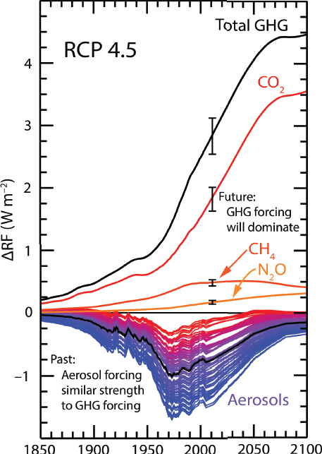
Hence, identifying aerosol’s influence on past and present climate is critical to establishing the potential future warming.
Current uncertainties in projecting future responses of the Earth system to rising levels of GHGs represent a quantifiably huge economic and societal liability. Investments in resilient infrastructure will depend strongly on the magnitude and rate of the planet’s response to increasing greenhouse gases (e.g., infrastructure commitments to accommodate sea-level rise). Hence, the panel identified as a Very Important priority continuing and new measurements aimed at obtaining the information needed on aerosol radiative forcing to substantially reduce this uncertainty. Prior work (e.g., IPCC WG1, 2013) indicates that the radiative forcing uncertainty by aerosols (about 1 W m-2) is approximately twice that of any other single factor contributing to the estimated total forcing uncertainty (IPCC WG1, 2013). The IPCC report indicates the total forcing uncertainty to be approximately the same magnitude as the aerosol forcing uncertainty. IPCC WG1 Figure 8.16 and surrounding text indicate total forcing uncertainty is dominated by aerosol forcing uncertainty. Hence, at least a factor of 2 reduction in the uncertainty of radiative forcing of climate due to aerosols would be required to achieve a factor of 2 reduction in total forcing uncertainty, assuming contributing errors add in quadrature. This reduction would contribute to narrowing the estimate of the ECS, and hence results in tangible economic and societal benefits as noted in the subsection “C2: Climate Feedbacks and Sensitivity.”
Science Question and Application Goals
The overarching science questions for this subsection feed into Objective C-2h of the “C:2: Climate Feedbacks and Sensitivity” subsection.
Question C-5. A. How do changes in aerosols (including their interactions with clouds, which constitute the largest uncertainty in total climate forcing) affect Earth’s radiation budget and offset the warming due to greenhouse gases? B. How can we better quantify the magnitude and variability of the emissions of natural aerosols, and the anthropogenic aerosol signal that modifies the natural one, so that we can better understand the response of climate to its various forcings?
In this subsection, we address the fundamental aspects of these questions that are related to aerosols—naturally and anthropogenically derived—the processes that govern their atmospheric burdens, and their interactions with clouds. For this subsection, there are four closely related objectives:
- C-5a. Improve estimates of the emissions of natural and anthropogenic aerosols and their precursors via observational constraints (Very Important).
- C-5b. Characterize the properties and distribution in the atmosphere of natural and anthropogenic aerosols, including properties that affect their ability to interact with and modify clouds and radiation (Important).
- C-5c. Quantify the effect that aerosol has on cloud formation, cloud height, and cloud properties (reflectivity, lifetime, cloud phase), including semidirect effects (Very Important).
- C-5d. Quantify the effect of aerosol-induced cloud changes on radiative fluxes (reduction in uncertainty by a factor of 2) and impact on climate (circulation, precipitation) (Important).
What Are the Largest Uncertainties in Aerosol Direct Radiative Forcing?
The Earth observing missions that have been carried out over the past two decades have provided a wealth of data on global aerosol emissions, transport, and distributions, from anthropogenic pollution to
sea spray, volcanic emissions, smoke, and dust. These observations have been used to refine regional to global-scale models, and aerosol forecasts that assimilate such data show a remarkable ability to predict the locations and even surface concentrations of particulate matter in many cases (Al-Saadi et al., 2005). Spaceborne measurements have provided global distributions of aerosol optical depth (Remer et al., 2008) and some information on aerosol types (R. Kahn et al., 2007), complemented by comparison with Aerosol Robotic Network (AERONET) surface-based observations, as well as yielded an estimate of direct radiative forcing of climate due to aerosols (R. Kahn, 2012). However, the vertical distributions of aerosols are not constrained by column measurements of aerosol optical depth, yet these have an impact on the radiation budget. This is especially true of absorbing aerosols, for which large uncertainties dominate current overall understanding of the direct effect (Bond et al., 2013). Lidar measurements (Winker et al., 2009) have proven helpful in providing information that locates aerosol layers, but the lidar retrievals rely on a priori estimates of the aerosol type and properties. Further, better sensitivity is needed for accurate lidar retrievals near the surface, under conditions of low aerosol loadings, and in cloudy atmospheres. Last, improved retrieval of aerosol absorption (e.g., single scattering albedo), a significant climate parameter, is necessary. A possible pathway is combining optical depth measurements with advanced lidar techniques (e.g., High Spectral Resolution Lidar [HSRL]) and algorithms to yield a more accurate physical interpretation of the aerosol characteristics.
What Are the Largest Uncertainties in Aerosol Indirect Radiative Forcing?
Understanding aerosol-cloud-precipitation interactions from space is a complex problem, as it is fundamentally challenging or impossible to observe both the aerosol and the clouds in the same column. Adding to the complexity are the spatial scales in the problem, with an extent from micrometers to kilometers in terms of the totality of the effect and with variations across different meteorological conditions. Despite this, progress has been made in understanding how the properties of low warm clouds—generally considered to be the most susceptible to changes in available cloud-nucleating particles, and to have the largest impact on albedo due to their persistence and extent—are modified by increases in boundary layer aerosol concentrations (IPCC WG1). With the ability to detect drizzle (Stephens et al., 2008), the connections between aerosol, cloud properties, and precipitation can also be made (Suzuki et al., 2011, 2013), key to developing a better understanding of several of the indirect effects beyond simply albedo changes. Understanding of aerosol-cold cloud impacts is poorer, largely because of gaps in the knowledge on ice nucleation and the ability to identify the precise role of aerosols—for example, initial ice formation in relatively warmer cold clouds may hinge upon the presence of ice nucleating particles (Lohmann and Diehl, 2006; Storelvmo et al., 2011) and the ability to detect and quantify them. Further, current methods do not accurately detect the onset of precipitation (ice crystals or light snow) in low cold clouds (Skofronick-Jackson et al., 2013).
Effects of particles on convective clouds have also been hypothesized using models (Morrison and Grabowski, 2011; Song and Zhang, 2011). Observable outcomes of such effects include changes in updraft strength, modified precipitation, and changes in cloud anvil properties and extent (Koren et al., 2005, 2010; Wang and Feingold, 2009; Saleeby et al., 2015), and thus a strategy targeted at indirect effects in convective clouds must include these as observable variables (Seinfeld et al., 2016).
For all aerosol indirect effects, the environmental conditions under which the cloud forms are also key to shaping the aerosol impacts (Comstock et al., 2005; Fan et al., 2009; VanZanten et al., 2011) and must be characterized close to simultaneously with the aerosol and cloud fields.
Measurement Objectives and Approaches
- Aerosol direct radiative effects. The POR will include instrumentation (VIIRS) that continues the record of radiometer measurements that can be used to derive aerosol optical depths. Further, new instruments such as Geostationary Orbit Environmental Satellite-R Series (GOES-R) provide similar, high-resolution geostationary data with high time resolution. The addition of capabilities for vertical distribution of the aerosol column, and for improving estimates of spectral aerosol absorption, is required to address the science objectives. At a minimum CALIPSO-like lidar and polarimeter will be needed. These observations, combined with other continuing or new instruments, will be useful in addressing the objectives.
- Aerosol indirect effect. Since atmospheric aerosols serve as the nuclei for cloud particles and hence exert a strong influence on cloud formation, microphysics, and precipitation—that is, the hydrologic cycle—aerosol indirect effects are manifest in a continuous arc that begins with how, when, and where aerosol are ingested into clouds, and ends with their removal to the surface in precipitation or resuspension in the atmosphere after processing, along with the changes to the atmospheric state induced that then feed back into subsequent cloud cycles. Clearly, this highly coupled system is too complex and operates on too many scales to permit direct observation of all individual processes. The panel defined an approach to knowledge generation that prioritizes an observational strategy emphasizing the characterization of cloud microphysics and precipitation, especially properties that have been hypothesized to respond to changes in the nature and amount of atmospheric particulate matter. Importantly, the observations of clouds and precipitation must be put into the context of the ambient aerosol and environmental state conditions. Hence, the observational strategies put into place to address aerosol direct radiative effects (Objectives C-5a and C-5b) will serve the dual purpose of providing important observations addressing Objectives C-5c and C-5d. Inevitably, some information about the aerosol properties and three-dimensional (3D) distribution that is relevant to aerosol-cloud interactions must be provided by models. The observational strategy that places an emphasis on better characterization of emissions (Objective C-5a) will serve to improve our ability to model the atmospheric aerosol with greater fidelity and hence to provide the needed links between the aerosol environment and cloud formation and evolution.
The required observations of clouds and precipitation include a combination of the measurements indicated under “C-2: Climate Feedbacks and Sensitivity” (Question C-2) for clouds, together with the instruments named earlier for the aerosol radiative effect. While the precipitation issue, including drizzle effects as diagnosed recently from CloudSat observations (e.g., Suzuki et al., 2013), could be considered from an observational strategy perspective as an element separate from the measurement of the aerosol-induced cloud albedo changes, it is nevertheless important to synthesize the composite picture emerging from both sets of measurements for the complete description and quantification of the aerosol-cloud interactions. Cloud radars form a key component to fully document the cloud properties especially for precipitation onset, light drizzle, which would complement the other platforms providing precipitation data. The lidar capabilities outlined earlier will be useful for quantifying anvils and other thin, high clouds, as well as obtaining estimates of the coverage of low clouds, many of which are missed by the spaceborne radars currently operating or envisioned. We need better information on cloud phase so that we can better describe the overall microphysical processes at play in both stratiform and convective clouds, and then make a link back to the aerosol that affects these. We need to characterize anvil and other thin-cloud prevalence and properties because of their radiative effects, and also because there are hypothesized indirect effects manifested in the anvil and thin-cloud characteristics. Cloud fraction responses to absorbing aerosol could
also be examined, when the aerosol environment is known or modeled well, as suggested here. Effects of aerosol on microphysics and in turn, on the strength of convection can be studied if observations of in-cloud vertical motion are available.
There needs to be a very strong linkage to suborbital programs such as DOE ARM and NASA AERONET. Venture-class missions can also be helpful in filling observational gaps. Dedicated field campaigns that augment space-based observations would strengthen the quantification of the aerosol indirect forcing and thus the net anthropogenic forcing. In addition, the combination of models (high-resolution global climate models [GCMs], cloud resolving models [CRMs], and large eddy simulations [LESs]), and in situ observations, together with the space-based observations, will be needed to quantify this effect globally. It is likely that only such a combination of platforms would resolve the roles of the naturally occurring and anthropogenic aerosols on clouds.
Connections to Other Panels and Integrating Themes
Weather and Air Quality Panel
Aerosols are a huge public health issue. Improved detection closer to the surface has relevance to health as well as to safety issues surrounding the transportation sector. Other related effects include aerosol effects on aviation and tourism.
Ecosystems Panel
Some sources of aerosols cause acid rain, which damages ecosystems. This is under control in the United States and most of Europe, but a growing problem in the developing world. Deposition of dust and black carbon is believed to accelerate melting of ice and snowpack.
Water and Energy Cycle
Effects on precipitation will directly impact these cycles.
C-6 and C-7: Seasonal-to-Decadal Predictions, Including Changes and Extremes
Motivation
Variations in the climate system on the scale of seasons to decades have substantial impacts on human life and on the economic and infrastructural health of society. Precipitation deficits that lead to droughts, for example, affect water and food supplies. Floods, arising from precipitation excess, lead to immense destruction. Coastal regions experience severe inundation from storm surges occurring amid rising sea levels and high tides (see also Question C-1, under “Relevant Climate Topics,” earlier). Abnormally hot summers laden with heat waves can have detrimental impacts on human mortality and on ecosystems (e.g., forests), while abnormally wet periods can foster the spread of mosquito-borne disease. Arctic sea-ice cover varies from year to year with large amplitudes, affecting transportation, commerce, and local ecosystems. On the longer (decadal) time scales, oceanic variations can imprint themselves on atmospheric weather patterns, leading to seasonal- and decadal-scale regional shifts and changes in the occurrence of good weather, drought, and so on. Meteorological patterns such as the stagnation of high-pressure systems can give rise to continental-scale heat waves, and the El Niño cycle can induce rainfall excesses or deficits across the globe. Oceanic currents along coasts, which cause disruptions in coastal activities and fisheries, are driven both by natural variability and by forcing of the Earth system.
If we could predict such variations ahead of time—either specific, transient anomalies at the seasonal-to-interannual scale or, at the decadal scale, shifts or trends in the nature of the atmospheric and oceanic circulation and the associated probabilities of extremes—we could prepare and plan for them sufficiently early and could adapt to or mitigate their ill effects, leading to reduced damages and enhancing significantly economic and health benefits. As an example, predicting Arctic ice conditions in a given year can guide local storm risk assessments, planning for village resupply, and so on, and learning about the Arctic being generally ice-free during summer in coming decades would present unprecedented opportunities in a variety of economic and commerce sectors. In general, across the globe, skillful predictions of fair or problematic weather and climate, and associated risks of weather and climate extremes, would substantially support short-term and long-term planning in agriculture, the military, aviation, tourism, water and land management, and so on. Over the past decade significant advances have been made in the observation of the important variables and in the development of modeling and assimilation systems, all key to improved prediction systems.
To fully realize the benefits, however, we must address a number of currently unanswered questions. For example, have we adequately tapped all relevant sources of predictability in the Earth system, and are our modeling systems realistic enough to translate this information into forecast skill? Regarding longer time-scale variability, how will the Hadley and Walker weather circulations change in the coming decades? Will the monsoon systems in different regions of the world exhibit a shift in amplitude and spatial extent? Is the character of the Atlantic Meridional Overturning Circulation (AMOC) changing? Such circulation patterns can vary naturally on long time scales but may also respond to imposed external forcing (e.g., increases in CO2, methane, nitrous oxide, halocarbons, and aerosols). The decadal-scale aspect of the prediction problem indeed represents a new challenge to both science and societal planning. Scientists recognize it as both an initial value problem (forecasted decadal-scale anomalies partly reflect the state of the system at the start of the forecast) and a boundary value problem (the decadal-scale anomalies also reflect the evolution of CO2, methane, aerosols, and other forcings that are anthropogenic in origin; IPCC WG1, 2013). Figure 9.14 illustrates hindcast simulations using a coupled climate model and a data assimilation system to demonstrate the significance of both observed initial conditions and radiative forc-
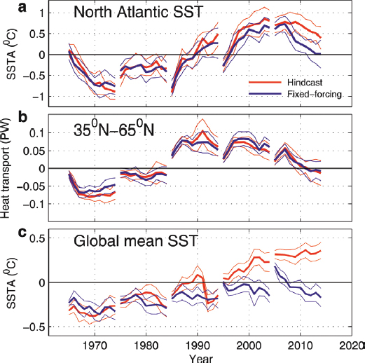
ing of climate on decadal predictions (Yang et al., 2013). While the global SST is driven by the radiative forcings, the decadal-scale North Atlantic SST and heat transport in the midlatitudes are driven primarily by the initial conditions.
The decadal problem is in fact new ground for consideration in the sustained monitoring of the Earth system, since it extends beyond both traditional weather forecasting (almost exclusively an initial-value challenge, at least to weekly and perhaps even to subseasonal time scales) and studies of decadal-to-centennial-scale climate change (boundary value problem). Societal planners and decision makers recognize the decadal scale problem as affecting infrastructural planning; such planning constitutes large resource investments and thus demands accurate, credible predictions. Planners are interested in knowing the potential for extremes (e.g., temperature, precipitation) as much as the mean trends.
The chief tools currently used for seasonal-to-decadal prediction are numerical models of the climate system—models that simulate the coupled behavior of the ocean, biosphere, cryosphere, and atmosphere (see Figure 9.1). The coupled models act to translate the information content of the initial state of the system into predictions of, for example, seasonal temperature and precipitation in continental regions or the extent of sea ice. Figure 9.15 provides an example of skill levels achieved with such a forecasting system. The coupled models can also simulate the impact of the boundary forcing (CO2 concentrations, aerosols, etc.) on circulation patterns. In addition to the deployment of coupled global general circulation model prediction systems, some problems will require additional tools to estimate the physical impacts. For example, in the risk analysis of coastal inundation due to sea-level rise, tides, and storm surges, well-documented tools such as wave and tidal models, along with fine-grained regional coastal models, will be additionally needed.
A measurement program that includes satellites and that is complemented by adequate surface-based and other in situ observational platforms will contribute comprehensively to the initialization of Earth system models and thus to the skill of forecasts. In addition, sustained monitoring of variables that describe the evolution of the external forcing would allow us to better characterize the evolution of Earth’s general circulation patterns and thereby enable tackling both the initial and boundary value aspects of the seasonal-to-decadal forecast problem.
In essence, the seasonal-to-decadal problem involves the quantification and prediction of “weather” anomalies, including extremes, superposed on a changing climate that is itself governed by natural and
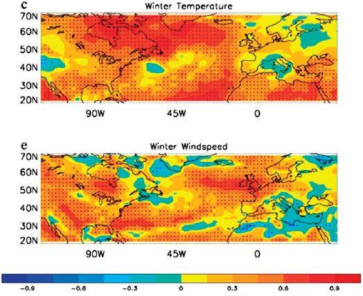
anthropogenic forcings on the Earth system. The present maturity of the science and of existing measurement and instrumentation techniques provides confidence in meeting this challenge over the next decade.
Science Questions and Application Goals
Question C-6. Can we significantly improve seasonal to decadal forecasts of societally relevant climate variables?
Question C-7. How are decadal-scale global atmospheric and ocean circulation patterns changing, and what are the effects of these changes on seasonal climate processes, extreme events, and longer term environmental change?
The SATM (see Appendix B, Questions C-6 and C-7) describes the overarching and most societally relevant questions in the seasonal-to-decadal prediction challenge. These questions relate to the prediction of climate variations seasons to decades ahead, the identification and prediction of variations and trends in large-scale weather and ocean patterns that could lead, for example, to regime shifts in temperature and precipitation, and the determination of associated shifts in the occurrence and character of extreme events.
The SATM lists the specific goals associated with these questions. For seasonal-to-decadal prediction, the goals are to produce improved initial ocean states (including cryospheric components), land states (including cryospheric components), and stratosphere states for forecasts, as follows:
- C-6a. Decrease uncertainty (by a factor of 2) in the quantification of surface and subsurface ocean states for initialization of seasonal-to-decadal forecasts (Very Important).
- C-6b. Decrease uncertainty, by a factor of 2, in quantification of land surface states for initialization of seasonal forecasts (Important).
- C-6c. Decrease uncertainty, by a factor of 2, in quantification of stratospheric states for initialization of seasonal-to-decadal forecasts (Important).
Initializing ocean states is critical because these states impart the greatest predictability to the Earth system. Ocean heat content, particularly in the subsurface, has substantial memory and underlies our hopes for reliable decadal scale prediction and for most facets of seasonal-to-interannual prediction. The phases of the El Niño Southern Oscillation cycle (ENSO; a coupled mode of the atmosphere-ocean system), for example, can be predicted months or more in advance if the ocean is properly initialized; recent model experiments suggest (X. Yang, personal communication) that initializations that utilized observed subsurface oceanic profiles prove crucial for hindcasting of the 2015-2016 El Niño. (Note that the arbitrary specificity of the phrase “by a factor of 2” reflects the unique character of the seasonal-to-decadal [S2D] prediction problem, for which precise skill improvements cannot be specified; see the following.)
For questions regarding the atmospheric circulation, the SATM lists several objectives, as follows:
- C-7a. Quantify the changes in the atmospheric and oceanic circulation patterns, reducing the uncertainty by a factor of 2, with desired confidence levels of 67 percent (likely in IPCC parlance) (Very Important).
- C-7b. Quantify the linkage between natural (e.g., volcanic) and anthropogenic (greenhouse gases, aerosols, land use) forcings and oscillations in the climate system (e.g., MJO, NAO, ENSO, QBO). Reduce the uncertainty by a factor of 2. Confidence levels desired: 67 percent (Important).
- C-7c. Quantify the linkage between global climate sensitivity and circulation change on regional scales, including the occurrence of extremes and abrupt changes. Quantify the expansion of the Hadley cell to within 0.5 degree latitude per decade (67 percent confidence desired); changes in the strength of AMOC to within 5 percent per decade (67 percent confidence desired); changes in ENSO spatial patterns, amplitude, and phase (67 percent confidence desired) (Very Important).
- C-7d. Quantify the linkage between the dynamical and thermodynamic state of the ocean upon atmospheric weather patterns on decadal time scales. Reduce the uncertainty by a factor of 2 (relative to decadal prediction uncertainty in IPCC, 2013). Confidence level: 67 percent (likely) (Important).
- C-7e. Provide observational verification of models used for climate projections. Are the models simulating the observed evolution of the large-scale patterns in the atmosphere and ocean circulation, such as the frequency and magnitude of ENSO events, strength of AMOC, and the poleward expansion of the subtropical jet (to a 67 percent level correspondence with the observational data)? (Important).
The two Very Important objectives address the aspects of decadal-scale variability in atmospheric circulation most relevant to society: how changes in the circulation affect mean weather conditions and, just as important, how they affect the probability of weather extremes such as droughts, floods, and hurricanes. Existing research has demonstrated the importance of observations combined with state-of-the-art modeling and assimilation systems to the analysis of such extremes; Murakami et al. (2015), for example, describe successful hindcast simulations of hurricanes in the world’s ocean basins over the past ~3 decades, including the most destructive Category 4 and 5 storms. With expected advances in observations, the science is well poised to address decadal-scale changes in the character of circulation and extremes.
Measurement Objectives and Approaches
The S2D prediction problem is best addressed by evaluating and improving the predictions made with forecast modeling systems and through climate studies utilizing state-of-the-art decadal-centennial climate models. These models should indeed provide the best, and most relevant, S2D forecasts of extremes and shifts in climate patterns, particularly if initialized with continuous space-based measurements in conjunction with complementary in situ and airborne measurements.
For S2D prediction (Question C-6 in the SATM), the measurement objectives targeted here are associated with forecast model initialization, which in the coming years will rely on the IESA framework. As discussed earlier, the IESA is a coupled model data assimilation system that ingests and optimally combines a wide variety of data sets into a single consistent and comprehensive picture of atmospheric, ocean, cryospheric, and land states. (This comprehensive modeling framework will indeed serve as a basis for much of NASA Earth science in the coming years.) The IESA can thereby provide estimates of ocean, land, and stratosphere states (including cryospheric components) that are critical for initializing forecasts extending beyond the ~10-day scale of weather prediction. Among the measurements that should be ingested into IESA systems for the S2D prediction problem are the following:
- Tropospheric quantities (temperature, water vapor, cloud properties, tropospheric winds, surface pressure);
- Stratospheric quantities (polar vortex winds, ozone, temperature, water vapor);
- Ocean quantities (sea-surface height, sea-surface salinity, sea-ice thickness, sea-ice fraction, sea-surface temperature, surface vector winds, subsurface temperatures and salinity, surface currents, ocean mass, ice-shelf slope); and
- Land-surface quantities (soil moisture at the surface and in the root zone, freeze-thaw state, total water storage, vegetation phenology, snow water amounts, surface albedo).
The SATM provides information on optimal resolutions and approaches.
Characterizing decadal-scale shifts in climate patterns (Question C-7 in the SATM) requires continuous space-based measurements examined in the context of the new generation of global numerical models that couple together the atmosphere, oceans, biosphere, and cryosphere. Needed measurements include the following:
- Climatological averages and anomalies in weather patterns (e.g., Arctic wintertime winds, midlatitude jets, surface and subsurface ocean currents, water vapor transport, cloud distributions) and surface meteorological variables (e.g., precipitation, air temperature, soil moisture).
- Natural (volcanic, solar) and anthropogenic (greenhouse gases, aerosols, land use) forcings. For the short-lived forcers in particular, the precursor emissions together with a self-consistent meteorology would be needed to obtain accurate global distributions and thus the spatially dependent forcings.
- Atmospheric circulation on regional scales including the occurrence of extremes and abrupt changes.
- Dynamic and thermodynamic state of the ocean.
- Evolution of the large-scale patterns in the atmosphere and ocean circulation (e.g., ENSO, AMOC, poleward shift of the subtropical jet).
For both questions, a large variety of measurement types are listed here. This underlines the unique character of these questions and their associated objectives: because the variety of measurements far exceeds what can reasonably be expected from a single NASA mission, answering either question is probably best viewed not as the motivation for a specific mission. Instead, it is best considered as benefiting (e.g., via integration through the IESA) from a very wide range of measurements collected in response to missions designed for other science objectives (e.g., the measurement of sea-surface height for the study of sea-level rise or the measurement of cloud information needed for determining climate sensitivity). Another motivation for this viewpoint is the fact that the limits of predictability on seasonal to decadal time scales are currently difficult to quantify (NRC, 2010), so quantitative promises cannot be made regarding skill improvements associated with any specific measurement. Note, however, that the consensus in the scientific community is that current forecast systems fall short of the predictability limits due in part to deficiencies in forecast model initialization and in the models themselves, and that an improved measurement program would significantly mitigate the first deficiency. Quantitative reduction of uncertainties along with the desired confidence levels indicated in the objectives stated earlier serve as markers to be attained in the S2D challenge.
Given the use of the IESA for forecast initialization, two aspects of the listed measurement objectives for the S2D forecast problem require consideration:
- The absence of any particular measurement is not a “deal-breaker,” since some value is still derived from the others through the IESA’s integration. Note, however, that sea-surface height, sea-surface temperature, subsurface temperatures, surface vector winds, and surface currents in the ocean and root zone soil moisture and snow at the land surface are considered by some to be most important for seasonal prediction, whereas for decadal prediction (and seasonal sea-ice prediction), important variables also include salinity, sea-ice thickness, sea-ice fraction, and ocean mass.
- While the particular spatial resolutions listed for this objective in the SATM, which were compiled through discussion with experts in the field, can be considered optimal targets, coarser resolutions than those listed would also not be deal-breakers, since useful information that advances understanding and prediction could still be extracted from the coarser data.
The key point is that the accuracy of the model assimilation product (for initialization of the forecasts and for the analysis of seasonal-to-decadal variations) should improve as the variety of the data sets employed increases and as the resolution of each data set used increases. Such a pathway from improved measurements to improved data assimilation products (both through the direct ingestion of the measurements into the data assimilation system and through their use in improving the system’s underlying models) has been demonstrated extensively—for example, in the context of initializing numerical weather forecasts (e.g., Dee et al., 2014). The S2D problem should benefit, to varying degrees, from newly captured measurements obtained in a number of NASA missions.
Because of the continuum of time scales—from seasonal to interannual to decadal—being dealt with for questions C-6 and C-7, and given the urgent need for the U.S. weather and climate communities to tackle and successfully address “seamlessness” in weather-to-climate forecasting (e.g., NRC, 2012), continuity in observations and sustained measurements are essential. This is particularly true given the need to address not only “average” weather but also its extremes (the “tails” of the probability distribution function of atmospheric and ocean states).
While many of the needed measurements are amenable to satellite-based remote sensing (and are in fact covered by the Program of Record), some are not; subsurface ocean temperature distributions, for example, must presumably be measured with in situ buoy systems or through the Argo array (including Deep Argo). Field campaigns may be needed to characterize relevant processes related to well-mixed and short-lived greenhouse gases, aerosols, clouds, and wind fields. For the boundary-value component of the decadal problem, it will also be necessary to quantify relevant external forcings (CO2 concentrations, etc.). While satellite data can contribute to estimates of, for example, precipitation and land use, supplementary ground-based measurements can significantly bolster such estimates. Of the satellite-based measurements needed, the measurement type not addressed within the POR is ocean surface currents, which would require the development of a Doppler scatterometer. Importantly, reanalysis (IESA) will be needed to assemble a comprehensive time series of states for complete Earth system determination.
A key aspect to consider in the seasonal-to-decadal forecasting problem is the joint requirement of accurate initial conditions (as provided by the IESA) and a model for evolving the initial states forward in time. Forecast models are far from perfect, and thus model physics development would be valuable in conjunction with improved initial conditions. Such model development (particularly, improvements in process parameterizations) would presumably benefit from a wide variety of NASA measurements.
The need for an IESA is part of an overall need here for coupled data assimilation, initialization, reanalyses, and reforecasts. There has been exceedingly good progress in IESA development, particularly involving the physical climate system, over the last decade. Addressing the S2D problem correctly, however, will require more than making routine accurate forecasts based on sustained observations of climate parameters around the globe. In the future modeling the coupled physical climate system in isolation will be increasingly insufficient; the coupling will need to be expanded to include biogeochemical cycles (carbon, nitrogen, etc.) and terrestrial and marine ecosystems. The challenge then becomes more complex given the corresponding expansion of the catalog of variables to be observed. However, the resultant outcomes should provide powerful and gainful benefits for multiple societal sectors.
Connections to Other Panels and Integrating Themes
The seasonal-to-decadal forecasting problem and the weather-climate interface challenge it entails has a strong tie to the subseasonal, regional forecasting objectives of the Weather Panel (Questions W-2 and W-4); the drought and water-related forecasting objectives of the Hydrology Panel (Questions H-1 to H-3) and sea-level-related coastal impacts (Question H-4); and the weather/climate-driven cycling of key constituents (e.g., water, carbon) among the priorities of the Ecosystems Panel (Question E-2). Also, an external forcing mechanism that can affect circulation patterns is solar irradiance changes and the loading of the stratosphere with sulfate aerosols following explosive volcanic eruptions. The occurrence of explosive eruptions has a potential link with Earth’s surface dynamics priority of the Solid Earth Panel (Questions S-1 and S-4); coastal loss due to sea-level rise (SLR) has a potential link with Question S-3. The prediction of temperature and precipitation and sea-ice anomalies at seasonal and longer time scales ties in directly to the Water and Energy Cycle Integrating Theme, and the prediction of changes in the character of extremes has an obvious linkage with the Integrating Theme on Extremes.
C-8: Causes and Effects of Polar Amplification
Motivation
Polar amplification refers to the potential for greater warming in polar regions compared to the rest of the globe due in part to strong positive feedbacks between ice cover and albedo decreases and air temperature increases in these regions causing additional warming. In the Arctic amplification is already observed, while for the Antarctic amplification does not seem to be in effect yet due to the presence of dampening processes. While polar amplification is largely driven by changes in sea ice and snow cover, changes in atmospheric and ocean circulation, including changes in prevailing winds driven by ozone depletion, have also contributed. Understanding these processes and their impacts on the global climate is critical to understanding climate sensitivity. Changes in the polar regions may affect global climate through changes in ice coverage, clouds, winds, carbon pools and fluxes, bottom water formation, and sea-level rise.
While polar regions are remote, they are relevant to global climate and human systems. Polar regions are generally covered by snow and ice most of the year, helping to keep the planet cooler than it otherwise may be. These regions are key in the formation of deep ocean water that drives global ocean circulation patterns, as well as driving large-scale atmospheric circulation between the warm tropics and the cold poles. Today, we are seeing pronounced changes in the polar regions, which climate models have struggled to accurately simulate. In most cases models have been too conservative in their projections of cyrospheric change, especially in regard to the Arctic sea-ice cover (Stroeve et al., 2007, 2012), but also in regard to changes in northern hemisphere snow cover (Derksen and Brown, 2012) and ice-sheet flow (Pollard et al., 2015). This is due to a range of key processes that are not fully understood or not accurately represented in the models, resulting in considerable model deficiencies.
Arctic temperatures have continued to rise at two to three times the rate of global temperature increase, with the average annual surface air temperature anomaly over land north of 60°N for October 2015-September 2016 being 3.5°C above preindustrial levels (Richter-Menge et al., 2016). In response to this rapid warming, Arctic sea-ice cover in the month of September has declined by nearly 14 percent per decade, as documented by nearly four decades of satellite observations (IPCC AR5, 2013). Earlier ship and aircraft observations, whaling log reports, and ice charts reveal that today’s sea-ice loss in the Arctic is unprecedented in the last 150 years, while sea-ice reconstructions from terrestrial proxies suggest it is unprecedented in at least 1450 years (Kinnard et al., 2011). Similarly, long satellite records have documented a significant reduction in seasonal snow cover extent over recent decades (Derksen and Brown,
2012); the rapid loss of land ice from Greenland (Shepherd et al., 2012) and glaciers and ice caps from Alaska, Canadian Arctic, Russian Arctic, Svalbard, Iceland (Jacob et al., 2012); and an increase in coastal erosion along Arctic permafrost shores (Jones et al., 2009). These changes have already affected Earth’s radiation budget, raised sea level, and affected land water hydrology, coastal erosion, marine ecosystems, the Arctic atmosphere, and the carbon cycle.
There has also been rapid warming of the Antarctic Peninsula and rapid melt of West and East Antarctic ice. The Antarctic Circumpolar Current has warmed faster than the global ocean as a whole, which plays an important role in the carbon budget. On the other hand, warming for the Antarctic continent has been much slower than Arctic warming. Ozone depletion from human activities is part of the explanation, leading to intensification of the polar vortex and strengthening of the westerly winds. This has effectively isolated Antarctica from warming elsewhere on the planet, leading to little change in surface temperature over much of the Antarctic continent. Changes in the winds have also largely driven the slight expansion of Antarctic sea ice over the satellite data record, although the last 2 years have seen record low, or near record lows, highlighting the large interannual variability in the Antarctic sea-ice cover. Uncertainty remains as to the role of natural versus forced climate variability in explaining the expansion (NASEM, 2017). Hence, unlike in the Arctic, where temperatures are increasing at 2-3 times the global average, the Antarctic has not warmed as fast as the rest of the world. Both climatic trends have, however, impacted the Earth system beyond the polar regions and have both contributed to sea-level rise from melting land ice.
Given these rapid changes taking place at the poles, there is an urgent need to observe and understand the changes taking place at high latitudes, especially in the Arctic, in order to help and protect human systems and support decision making, but also in the Antarctic, to understand its impact on global climate and sea-level change.
While anthropogenic influences have very likely contributed to Arctic sea-ice loss since 1979 (IPCC, 2013; Notz and Stroeve, 2016), the thinning and shrinking of the Arctic sea-ice cover combined with reductions in northern hemisphere snow cover in June has contributed to amplification of the warming in the northern polar regions (Serreze et al., 2009; Brown and Robinson, 2011; Derksen and Brown, 2012; Najafi et al., 2016). Changes in atmospheric and oceanic circulation, heat-trapping water vapor and clouds, and the lapse rate feedback, have also contributed, although uncertainty remains as to the relative contributions of each to the observed warming (Pithan and Mauritsen, 2014). The importance of the factors driving Arctic amplified warming is relevant in improving an understanding of whether and how continued Arctic change will impact midlatitude weather extremes or, at the very least, if the two phenomena are correlated. The chaos of the atmospheric circulation makes it difficult to determine whether or not amplified warming in the Arctic is already impacting midlatitude weather extremes. This topic is a major research challenge, yet continued monitoring Arctic changes, such as sea-ice loss and snow cover retreat, together with better characterization of the atmosphere can help to answer this question.
Much of the understanding and documentation of these changes come from decades of satellite observations. Continuation of these long-term satellite observations are essential for understanding the role of natural climate variability versus anthropogenic forcing on the long-term decline of sea ice, its impact on midlatitude weather, the impact of melting land ice on global sea level, and quantifications of hydrological and biogeochemical fluxes.
Science Question and Application Goals
Question C-8. What will be the consequences of amplified climate change already observed in the Arctic and projected for Antarctica on global trends of sea-level rise, atmospheric circulation, extreme weather events, global ocean circulation, and carbon fluxes?
In order to make progress on this science question, the panel has identified the following objectives:
- C-8a. Improve our understanding of the drivers behind polar amplification by quantifying the relative impact of snow/ice-albedo feedback versus changes in atmospheric and oceanic circulation, water vapor, and lapse rate feedback (Very Important).
- C-8b. Improve understanding of high-latitude variability and midlatitude weather linkages (impact on midlatitude extreme weather and changes in storm tracks from increased polar temperatures, loss of ice and snow cover extent, and changes in sea level from increased melting of ice sheets and glaciers) (Very Important).
- C-8c. Improve regional-scale seasonal to decadal predictability of Arctic and Antarctic sea-ice cover, including sea-ice fraction (within 5 percent), ice thickness (within 20 cm), and location of the ice edge (within 1 km), timing of ice retreat and ice advance (within 5 days) (Very Important).
- C-8d. Determine the changes in Southern Ocean carbon uptake due to climate change and associated atmosphere/ocean circulations (Very Important).
- C-8e. Determine how changes in atmospheric circulation, turbulent heat fluxes, sea-ice cover, freshwater input, and ocean general circulation affect bottom water formation (Important).
- C-8f. Determine how permafrost thaw-driven land cover changes affect turbulent heat fluxes, above- and belowground carbon pools, resulting greenhouse gas fluxes (carbon dioxide, methane) in the Arctic, as well as their impact on Arctic amplification (Important).
- C-8g. Determine the amount of pollutants (e.g., black carbon, soot from fires, and other aerosols and dust) transported into polar regions and their impacts on snow and ice melt (Important).
- C-8h. Quantify high-latitude, low-cloud representation, feedbacks, and linkages to global radiation (Important).
- C-8i. Quantify how increased fetch, sea-level rise, and permafrost thaw increase vulnerability of coastal communities to increased coastal inundation and erosion as winds and storms intensify (Important).
The panel also determined that improving and continuing to characterize land-ice melt, accumulation of snowfall and ice flow dynamics of the ice sheets, mountain glaciers and ice caps and the physical processes (surface melt from warm air temperatures, basal melt from warm ocean temperatures, calving mechanisms, basal sliding) that drive these changes and how they relate to global climate variables are also important (see Question C-1 for requirements).
Few field observations are collected in the polar regions, which remain the least well explored parts of the planet. All the preceding stated objectives are important and require substantial investments in field and remote sensing observations as well as modeling.
Measurement Objectives and Approaches
The measurements needed for these objectives are listed in the SATM (see Appendix B). Here, we highlight the measurements that are needed to achieve the Very Important objectives listed earlier. For land-ice monitoring (ice sheets, glaciers), a range of active and passive microwave instruments, lidars, and
gravimetric sensors will be needed to continue existing time series of land-ice volumes and fluxes (see Question C-1).
- Sea-ice concentration/extent/ice type/thickness. These measurements are key for air-sea fluxes, radiation budget, biological feedbacks, regional-scale S2D variability and midlatitude weather forecasts. In the Arctic this information is also required by coastal managers, shipping companies, and extractive industries. Thus, there is a strong need to ensure continuity of the multichannel passive microwave observations started in October 1978 as part of the Defense Meteorological Satellite Program but to be discontinued. The existing satellites are aging, including JAXA’s AMSR2, which now exceeds its nominal lifetime, and currently the United States is not planning any follow-on missions to ensure the continuity of this historical data set. These sensors are important for other climate variables, including rainfall, snow cover, ice-sheet melt, sea-surface temperatures, wind speed, and soil moisture, which are critical measurements for Very Important priority climate variables such as air-sea fluxes, sea-level rise, and seasonal to decadal predictability. There is also a strong need to improve upon the resolution of these instruments (25 km for SSMI and 10 km for AMSR2) to better delineate the ice edge and for marine applications such as ship routing. Sea-ice thickness will require a combination of laser altimetry (e.g., ICESat) and high-frequency radar interferometry topographic mapping (Ku-/Ka-band, e.g., SWOT) to provide data at 1 km resolution with a vertical precision of 3 cm or better. Combining sensors will allow for both retrieval of snow depth and ice thickness, which one sensor alone cannot achieve. CryoSat, AltiKa, and Sentinel-3 are already providing standard sea-ice thickness products with greater precision (albeit lower spatial resolution), and SMOS is providing thin-ice thickness.
- Snow cover extent/thickness/snow water equivalent. While continuity of the multichannel passive microwave series is desirable, other approaches combining radar interferometry mapping (Ku-/ Ka-band) or laser and radar altimetry should be pursued to provide higher resolution data and precision measurements of the temporal variability in surface height. Snow thickness and water equivalent are critical for land hydrology and permafrost studies. Snow depth on sea ice is currently not retrieved with satellites, although there is the potential to retrieve it using dual radar Ka- and Ku-band radar topographic mappers, combined laser and radar altimetry (i.e., collocated ICESat-2 and CryoSat-2), L-band radiometers, or radar interferometry techniques.
- Changes in ice sheets, glaciers, and ice caps. See Question C-1 for additional details.
- Atmospheric boundary layer (surface temperatures, temperature profiles, surface-air fluxes, water vapor, clouds). Daily at 25 km spatial resolution, 200 m vertical resolution in the planetary boundary layer (PBL) using IR and microwave sounders (e.g., AIRS, AMSU, ATMS), GNSS-RO.
- Sea-surface temperature, wind speed. For calculation of air-sea fluxes, the skin temperature of the sea surface is required at diurnal resolution and a few kilometers spatial resolution, within 0.1 K accuracy. The temporal and spatial variability should be similar for wind speed at a few kilometers spatial resolution, daily, 2 m/s uncertainty, via scatterometers (e.g., QuikSCAT).
- Freeze/thaw state of the nonglacierized circumpolar land surface. Observation of this state is important for quantifying carbon, energy, and water fluxes and how they affect land cover change. This variable is best addressed with passive microwave radiometers or synthetic aperture radars. There are no current operational measurements of active layer thickness from space; however, observations of seasonal freeze-thaw cycles and the range of associated thaw subsidence and frost heave due to water-ice phase transitions allows indirect assessments of active layer thickness. Permafrost cannot be directly observed with current spaceborne sensors, and quantifying the state of permafrost across regions requires relation of environmental surface variables (air and skin temperature, land
- cover, snow cover and density, freeze/thaw state) with models of subsurface temperatures and validation data from boreholes (Pastick et al., 2015; Westermann et al., 2017). Long-term land surface subsidence due to permafrost thaw can already be observed with spaceborne InSAR—TerraSAR-X (X-band), Radarsat, Sentinel-1, ERS (C-Band), PALSAR (L-Band)—and the full range of lidar instruments from terrestrial to airborne to spaceborne (ICESat; Jones et al., 2015), and observations need to be continued and expanded to larger spatial domains. Monitoring of erosion along permafrost coasts requires annual high-resolution optical and SAR image data sets with submeter to several meters ground resolution.
- Bottom water formation, carbon update. Required is information on wind speed (see earlier), sea-surface temperature (see earlier), polynya formation using passive microwave and synthetic aperture radar (km spatial resolution, daily temporal resolution), ocean subsurface temperature via Argo network with ice-avoiding capability and seal data, autonomous underwater vehicles (AUVs), and gliders, and rate of thinning of Antarctic ice shelves (via CryoSat and ICESat-2 polar altimetry, interferometric synthetic aperture radar, km spatial resolution, monthly resolution).
Connections to Other Panels and Integrating Themes
Snow extent, thickness, and water equivalent are relevant to the water and energy cycle. Thawing permafrost is relevant to high-latitude terrestrial ecosystems, affects water resources in the terrestrial Arctic, and can be a hazard to northern communities. Measurements of ice melt are relevant to sea-level rise and coastal impacts worldwide. Understanding of high-latitude climate and connection to midlatitude climate, improved seasonal sea-ice forecasts, and a better characterization of the atmospheric boundary layer in polar regions is relevant to improving weather forecasts. Sea-ice forecasts are also relevant for coastal communities, shipping companies and extractive industries. Sea ice, permafrost and active layer state, as well as snow extent and thickness are relevant for managing northern transportation infrastructure and ecosystems. Permafrost thaw and mobilization of previously frozen carbon is directly contributing to carbon cycle changes and observation strategies for monitoring greenhouse gas release on global scales thus also apply for permafrost regions.
C-9: Ozone and Other Trace Gases in the Stratosphere and Troposphere
Motivation
Earth’s ozone layer shields the surface from harmful ultraviolet (UV) radiation. The global ozone layer is in the process of a slow, long-term recovery from human release of CFCs and other harmful ozone-depleting substances (ODSs; WMO, 2014; Solomon et al., 2016). As the atmospheric levels of CFCs and ODSs decline, levels of stratospheric column ozone will be controlled in a rather complex manner by future atmospheric levels of CO2, CH4, and N2O (Eyring et al., 2013; Revell et al., 2015; see Figure 9.16). The possible future intensification of the strength of the Brewer Dobson circulation due to rising levels of greenhouse gases (GHGs; Butchart, 2014) will also be a key factor in determining the future thickness of Earth’s ozone layer and the resulting levels of UV radiation reaching the surface (WMO, 2014).
In addition to controlling the transmission of UV radiation, stratospheric ozone is radiatively active and impacts atmospheric temperatures and circulation. The global radiative forcing (RF) by stratospheric ozone from 1750 to 2011 is estimated as –0.05 (–0.15 to +0.05) W m-2 (IPCC, 2013). But effects on climate arising from ozone-depletion-induced changes in atmospheric circulation can be much more significant. For example, the past decline of Earth’s ozone layer has been associated with changes in surface tem-
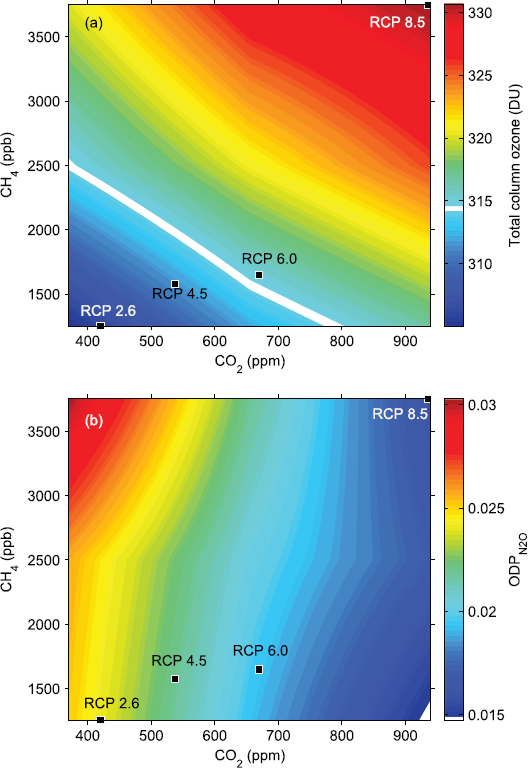
peratures, clouds, and precipitation in the southern hemisphere due to the Antarctic ozone hole (Previdi and Polvani, 2014). It has been suggested that the future recovery of the ozone layer will enhance surface warming globally in the first half of this century (Hu et al., 2011).
The stratosphere and troposphere are tightly coupled via the upper troposphere and lower stratosphere (UT/LS) region, commonly considered to be the region within ±5 km of the tropopause (Gettelman et al., 2011). The UT/LS plays a key role in controlling Earth’s radiative and thermal balance and climate (Gettelman et al., 2011; Riese et al., 2012; Coffey et al., 2014). But radiatively active species such as water vapor and ozone exhibit steep vertical gradients and substantial spatial and temporal variability in the UT/LS, leading to large uncertainties in quantifying their effects. The composition of this region is controlled by transport from the troposphere and stratosphere, and meridional exchange between the tropical UT and extratropical LS. Key issues involve the control of RF of climate due to changing levels of humidity (Solomon et al., 2010), aerosols (Kaufmann et al., 2011), and the response of temperature in this region to rising levels of GHGs (Gettelman et al., 2011).
Tropospheric ozone also exerts considerable control on climate. Human release of CO, NOx, and volatile organic chemicals (VOCs) has led to a buildup of tropospheric O3 (Shindell et al., 2006), which increased the global RF of climate by +0.4 (0.2 to 0.6) W m−2 between 1750 and 2011; this is almost equal to the RF of climate by CH4 (+0.48 Wm-2) over this same period of time (IPCC, 2013). The largest
contribution to the climatic influence of tropospheric O3 is from enhancements in the tropical troposphere (Stevenson et al., 2013). Elevated surface O3 adversely affects human health and agriculture (Avnery et al., 2011). Legislation enacted to protect public health has significantly reduced emissions of O3 precursors from automobiles, factories, and power plants throughout much of the industrialized world, resulting in a steady decline of tropospheric O3 levels in the extra-tropics (Cooper et al., 2014). It is unclear whether these will reduce the climatic impact of O3, since the largest radiative influence of O3 is in the tropics, where elevated O3 has been linked to biomass burning (Jacob et al., 1996; Anderson et al., 2016).
Science Question and Application Goals
Question C-9. How are the abundances of ozone and other trace gases in the stratosphere and troposphere changing, and what are the implications for Earth’s climate?
This can be answered with the following quantified objectives:
- C-9a. Quantify the amount of UV-B reaching the surface, and relate to changes in stratospheric ozone and atmospheric aerosols (Important).
- C-2g. Quantify the contribution of the upper troposphere and stratosphere (UTS) to climate feedbacks and change by determining how changes in UTS composition and temperature affect radiative forcing with a 1-sigma uncertainty of 0.05 W/m2 over the course of the decade (Very Important).
The goal here is to improve prediction of the ozone layer, as well as atmospheric and surface radiative forcing and its associated consequences for climate. Achieving this goal requires measurements of the temperature and changing composition in the UTS, including ozone and other radiatively active gases such as H2O, CO2, CH4, and N2O, as well as aerosols and aerosol precursors released by a wide variety of industrial processes, volcanoes, and biomass burning (aerosols are discussed in Question C-5). Distributions of O3 and other constituents that are key to climate predictability are controlled by chemical transformations, dynamical processes ranging from planetary and gravity waves to the Hadley Cell and Brewer Dobson Circulation, and the interaction of chemistry and transport (e.g., transport of pollutants in monsoonal circulations). Therefore, achieving this goal also requires knowledge of these processes, which means observing a suite of chemically reactive constituents such as NOx, HOx, and halogens, as well as transport tracers. It is also critical that existing suborbital assets such as (but in no way limited to) the Brewer Dobson Network, the Network for Detection of Atmospheric Composition Change, various programs that launch ozonesondes and watersondes, as well as routine (e.g., piggyback on commercial flights) and campaign observations by aircraft and balloons all be maintained. This will ensure that future spaceborne observations can be evaluated, eventually validated, and ultimately tied in a quantitatively meaningful manner to a wide variety of existing measurements. The ultimate, long-term goal is provision of climate data records that will allow the next generation of scientists to reliably assess, and confidently predict, the role of human activity on Earth’s protective ozone layer and consequences for surface UV, the consequences for climate of changes in Earth’s ozone layer, and the importance of the UT/LS region for climate change.
Measurement Objectives and Approaches
As detailed in the SATM (see Appendix B), improving predictability of the ozone layer and how changes in atmospheric trace gas concentrations will affect climate requires a complete set of measurements that
can be used to determine the vertically resolved distribution of stratospheric O3 and other trace gases from the upper troposphere through the stratosphere. These profiles must be measured with accuracy sufficient to quantify the decadal radiative forcing with a 1-s uncertainty of better than 0.05 W/m2. The SATM also includes an objective on quantifying the amount of UV-B radiation reaching the surface, since this is a quantitative measure of the impact of changing stratospheric ozone on the surface, even though this impact is not expected to be measured from space. For prognostic capabilities it is necessary to characterize the processes that control the UT/S temperature and constituent distributions, which requires measurements of relevant chemically reactive constituents and transport tracers. Observations of temperature and key radiatively active gases in the UT/LS must have sufficient precision, vertical resolution, and geographic coverage to quantify radiative forcing; the SATM requirements are specified to meet this requirement. In addition, diagnostics of the processes that control the temperature and distributions of O3 and other radiatively active constituents must be measured with a precision, vertical resolution, and geographic coverage appropriate for the scales on which the processes occur. As specified in the SATM, the observations must be global in nature, comprehensive, and with high vertical resolution (~1 km or better) because of steep vertical gradients in the UT/LS.
These measurement requirements can be met with a number of different approaches, each with advantages and disadvantages. For example, UV, visible, and infrared solar occultation (e.g., Mauldin et al., 1985; Russell et al., 1993; Lucke et al., 1999; Bernath et al., 2005) lend themselves to measurements with high-precision, sub-km vertical resolution, and climate-quality data; global coverage requires a constellation. Lunar (Amekudzi et al., 2005) and stellar (Kyrölä et al., 2004) occultation provide better horizontal coverage, but are less well-proven. Infrared (Fischer et al., 2008) and microwave (Waters et al., 2006) limb emission instruments provide global coverage with night and daytime sampling; obtaining fine vertical resolution is a challenge. Limb scattering of visible solar radiation (McPeters et al., 2000) is another technique that yields global coverage. Nadir-viewing instruments measuring emitted (Beer et al., 2001) or scattered (Bhartia et al., 1996) radiation can provide global coverage with very high horizontal resolution, but limited vertical resolution. Radio occultation measurements (Kursinski et al., 1997) have proven useful for tropospheric temperature and water vapor. Because of the rich spectrum of molecular lines, infrared sounders are typically capable of detecting more trace gas species than other instruments. All of these approaches have been used to measure ozone, temperature, or other trace gas species in the troposphere or stratosphere, and would be plausible candidates for contributing to the measurement objectives described earlier. The long-term plan in the United States for measuring vertical profiles of stratospheric ozone is to use the Ozone Mapper and Profiler Suite-Limb Profiler (OMPS-LP), but whether a succession of such instruments will be suitable for measuring ozone trends is not yet clear (Jaross et al., 2014).
Connections to Other Panels and Integrating Themes
Weather and Air Quality Panel
State-of-the-art operational forecast centers rely on models that assimilate satellite radiances. It has been shown that the stratosphere exerts a strong influence on tropospheric weather (Baldwin and Dunkerton, 2001; Kidston et al., 2015), and that medium and longer range weather forecasts exhibit quantitative improvement in accuracy when a realistic stratosphere is included in the forecast models (Baldwin et al., 2003; Charron et al., 2012; Sigmond et al., 2013). Also, downward transport of stratospheric O3 has been implicated in surface O3 violations, particularly during winter in mountainous regions such as the U.S. Midwest (Lin et al., 2015). Finally, poor air quality is known to occur during hot, stagnant conditions. Were stratospheric O3 recovery to accelerate global warming, then it would require even further reductions in the emission of O3 and aerosol precursors to achieve a particular air quality standard.
Societal Benefits
Earth’s O3 layer protects humans, animals, and plants from harmful ultraviolet radiation released by the sun, particularly in the UV-B spectral region (280 to 315 nm). The thickness of the global O3 layer was reduced by about 5 percent due to anthropogenic halogens in the early 1990s, which has and will continue to lead to excess skin cancer fatalities throughout the world (Slaper et al., 1996). The ban on the manufacture of ozone depleting substances brought about by the Montreal Protocol limited global O3 depletion at the ~5 percent level, thereby avoiding runaway increases in skin cancer due to a severely damaged ozone layer that could have otherwise resulted (Longstreth et al., 1998). The need to understand the effect of GHGs such as CH4 and N2O on the O3 layer is motivated by the societal importance of not reversing the great success of the Montreal Protocol.
The need to understand the radiative budget of the UT/LS is motivated, in part, by the fact that the RF of climate due to the rise in tropospheric O3 over the Industrial Era rivals that due to the rise in CH4 (see Figure 9.16), with most of this climate driver due to O3 increases in the tropical UT/LS. Simply put, it is unclear whether policy measures currently enacted or planned for the near future will reverse the trend of rising O3 in this climatically important region of the atmosphere. The tropical UT/LS has long been characterized as a nexus for the interaction of climate and atmospheric composition, and the conduit in the exchanges between stratospheric and tropospheric thermodynamical states. In addition, climate models poorly represent the processes that control the vertical distribution of radiatively active constituents in the UT/LS, even though changes in these constituents have a strong influence on the global climate (SPARC, 2010). The measurements described earlier are designed to provide data-driven policy options to address radiative forcing of climate that occurs in the UT/LS.
RESULTING SOCIETAL BENEFIT
Earth’s climate shapes the nature of societies, the characteristics of ecosystems and the performance of economies across the globe through its wide-ranging influence on natural and human systems (Carleton and Hsiang, 2016). What grows well, what prospers, where, and for how long depends on climate. Where it is more or less hazardous to live, whether because of risks of disease or natural hazard, depends on climate. The type of infrastructure needed to protect against natural hazards and ensure provision of energy, food, water, and transportation connectivity all depend on the climate.
As a result, many societal decisions—for financial investments, infrastructure design, natural resource management, and planning and policy making—are based in part on information, or assumptions, about expected climatic conditions. By improving our understanding of the current and future states of our climate, including climate sensitivity (see “C-2: Climate Feedbacks and Sensitivity”), improving our ability to predict fluctuations in climate, and improving our ability to detect important changes in our climate system, the priorities proposed here would enhance and strengthen society’s basis for decision making, thereby benefiting people and communities across the nation.
Like weather forecasts, anticipatory information about near-term climate has value for a wide range of decisions. Seasonal, interannual, and extending to decadal climate prediction (see “C-6 and C-7: Seasonal-to-Decadal Predictions”) are rapidly evolving areas of scientific research that rely on measurements of current ocean, land surface, sea-ice, and atmosphere conditions. Using these initial conditions, model predictions can be made for the phase and amplitude of many modes of variability in the climate system, including the El Nino Southern Oscillation (ENSO), the North Atlantic Oscillation (NAO), and the Pacific Decadal Oscillation (PDO); monsoons; departures from normal patterns; as well as the risk of extremes such as heat waves, hurricanes, floods, drought, or severe storms around the nation. These regionally and locally specific climate predictions, built in part upon improved atmosphere-ocean flux exchanges (see “C-4:
Atmosphere-Ocean Flux Quantification”), can be used for national-scale decisions about risk sharing (e.g., insurance or asset diversification), resource distribution (e.g., by energy companies in anticipation of altered patterns of energy demand for heating and cooling), capital investment decisions regarding seasonal recreation, disaster-response staging (NRC, 1999; AMS, 2003), and natural resource planning and management in specific locations (e.g., drought early warning, water resource management; Lettenmaier et al., 2003; NOAA/NIDIS, 2017). Improved regional seasonal-decadal prediction of Arctic and Antarctic sea-ice cover (see “C-8: Causes and Effects of Polar Amplification”) can inform planning by the shipping and fishing industries, while better quantification and projection of variability and changes in regional sea level can help coastal communities better predict their near- and longer-term risks of coastal erosion (see “C-1: Sea-level Rise”).
Information about what to expect, locally, as climate continues to change, including the possibility of rapid changes, is in increasing demand. At a global scale the current large uncertainties in climate change projections lead to a factor of 10 or more uncertainty in the magnitude of future long-term economic impacts (NRC, 2017). More locally, communities and businesses seek geographically targeted information to inform climate change risk and vulnerability assessments and decisions about short-, medium-, and long-term investments in protective adaptation and other climate change responses (Bierbaum et al., 2014). Planners, engineers, and natural resource managers facing decisions with long-term consequences desire improved information about the conditions expected over the lifetime of their project. For example, where, when, and for which health stressors or disease vectors should health departments design monitoring systems? How long can a city expect existing sources to supply sufficient drinking water for its citizens? How big must a reservoir be to ensure adequate irrigation water for new orchards? At what height must an interstate freeway be constructed to protect against increasing flood risk, and with which type of asphalt should it be constructed to withstand increasing heat (Iowa State University Institute for Transportation 2015, USDOT)? Coastal communities and infrastructure managers desire better estimates of the upper bound of sea-level rise for local risk assessments, infrastructure design, ecosystem protection and potential investment in relocation (e.g., Miami Herald, 2017,10 and San Francisco Chronicle, 201611). The fishing and aquaculture industry seeks improved information about future rates and hotspots of ocean acidification to inform hatchery and growing operations already tied to these conditions and early warning of other potential problem locations. Uncertainty about internal and naturally induced climate variations, and about the timing and magnitude of changes and their duration, are clear challenges to adaptation strategies with accompanying investment and risk considerations: urgent and unplanned-for adaptation incurs significant extra cost, while an investment in physical capital is largely irreversible, so investing too soon is also a cost that could be averted with reduction in uncertainties.
Improved climate change projections in general, and projections of sea-level rise, ocean acidification, and ozone in particular, will be supported by proposed work (see previous sections) on polar processes, aerosols, clouds and ozone, climate feedbacks and sensitivity, carbon cycle, atmosphere-ocean flux, sea-level rise, and ocean heat storage and glacier-ice. Improved understanding and prediction of climate changes from seasonal to centennial scales can be used to support decisions in nearly all sectors of society, with consequences on a wide spectrum of space and time scales. For example, it could be about when and how to manage planetary and regional climatic impacts, adaptation, and mitigation. Improved carbon-cycle monitoring (see “C-3: Carbon Cycle”) could help monitor accurately globe-wide sources (the development of an Integrated Global GHG Information System [IG3IS]12), and better quantify the emissions from all
___________________
10 See J. Flechas, 2017, “Miami Beach to Begin New $100 Million Flood Prevention Project in Face of Sea Level Rise,” Miami Herald, January 28, http://www.miamiherald.com/news/local/community/miami-dade/miami-beach/article129284119.html.
11 See J. King, 2016, “A Regional Response to the Bay’s Encroaching Waters,” Rising Reality, May, http://projects.sfchronicle.com/2016/sea-level-rise/part1/.
12 See P. DeCola, O. Tarasova, J. Butler, R. Duren, S. Reimann, K. Gurney, A. Manning, and the IG3IS Team, 2016, “Integrated Global GHG Information System (IG3IS): Evidence Based Policy Support and Evaluation: Paris Agreement on Climate Change,” September 22, http://carbon.nasa.gov/pdfs/DeCola_CMS_Policy_Sept22_16.pdf.
sources. Improved understanding of the ongoing effects of atmospheric gases on atmospheric ozone will help the nation ensure that the valuable gains in UV-protection afforded by the recovery of the ozone layer are maintained (see “C-9: Ozone and Other Trace Gases in the Stratosphere and Troposphere”). Improved monitoring of global and regional aerosol pollution together with information on meteorological conditions (see “C-5: Aerosols and Aerosol-Cloud Interactions”) is capable of yielding early warning information on heat waves and air quality, and the likely impacts to health and regional climates.
Observations of Earth’s climate system from space provide important real-time “nowcasts” of current conditions that inform weather forecasting, provide insight into evolving environmental threats or opportunities, and enable detection and early warning of severe climatic events. Ongoing measurements of atmospheric and oceanic conditions from space can improve midlatitude weather forecasts, in particular for extreme events. Information derived from enhanced monitoring of arctic sea-ice cover can help alert vulnerable arctic communities to near-term dangers of coastal inundation and flooding. Concomitant improved understanding of the connection between polar processes and global climate could help improve prediction and better calibrate the Arctic and Antarctic as “first indicators” of global climate change. Proposed measurements of biomass change, especially in the Arctic, are important for identifying release of carbon stored in permafrost, a potentially significant positive feedback to warming.
Full realization of these benefits will require concomitant advances in several related efforts to ensure that the observations, results, and products of the program described here are fully utilized across relevant arenas of science and society. Attention to measurement continuity and climate-quality measurements and data sets, including appropriate data archiving and metadata, is essential for understanding and predicting long-term changes in Earth’s climate. Continued investments in modeling are needed for observation assimilation, analysis, and evaluation, and for the crucial step of connecting these observations to information about changes in variables or systems of direct importance to society. Last, connecting the climate observing program described here to societal efforts to better anticipate, plan for, and adapt to climate fluctuations will require an effective information delivery system and robust forums. This will enable iterative interaction between the Earth-system observing community and the prospective scientific and public users of information derived from space-based climate-related observations (Miles et al., 2006).
REFERENCES
Ablain, M., J.F. Legeais, P. Prandi, M. Marcos, L. Fenoglio-Marc, H.B. Dieng, J. Benveniste, and A. Cazenave. 2017. Satellite altimetry-based sea level at global and regional scales. Surveys in Geophysics 38(1):7-31.
Abraham, J.P., M. Baringer, N.L. Bindoff, T. Boyer, L.J. Cheng, J.A. Church, J.L. Conroy, et al. 2013. A review of global ocean temperature observations: Implications for ocean heat content estimates and climate change. Reviews of Geophysics 51(3):450-483.
Al-Saadi, J., J. Szykman, R.B. Pierce, C. Kittaka, D. Neil, D.A. Chu, L. Remer, et al. 2005. Improving national air quality forecasts with satellite aerosol observations. Bulletin of the American Meteorological Society 86(9):1249-1261.
Amekudzi, L.K., A. Bracher, J. Meyer, A. Rozanov, H. Bovensmann, and J.P. Burrows. 2005. Lunar occultation with SCIAMACHY: First retrieval results. Advances in Space Research 36(5):906-914.
AMS (American Meteorological Society). 2003. Report of a Policy Forum: Improving Responses to Climate Predictions. https://www.ametsoc.org/ams/assets/File/Climate_response_2003.pdf.
Anderson, D.C., J.M. Nicely, R.J. Salawitch, T.P. Canty, R.R. Dickerson, T.F. Hanisco, G.M. Wolfe, et al. 2016. A pervasive role for biomass burning in tropical high ozone/low water structures. Nature Communications 7:10267.
Anderson, T.L., R.J. Charlson, S.E. Schwartz, R. Knutti, O. Boucher, H. Rodhe, and J. Heintzenberg. 2003. Atmospheric science: Climate forcing by aerosols—A hazy picture. Science 300(5622):1103-1104.
Avnery, S., D.L. Mauzerall, J. Liu, and L.W. Horowitz. 2011. Global crop yield reductions due to surface ozone exposure: 1. Year 2000 crop production losses and economic damage. Atmospheric Environment 45(13):2284-2296.
Baldwin, M.P., and T.J. Dunkerton. 2001. Stratospheric harbingers of anomalous weather regimes. Science 294(5542):581-584.
Baldwin, M.P., D.B. Stephenson, D.W.J. Thompson, T.J. Dunkerton, A.J. Charlton, and A. O’Neill. 2003. Stratospheric memory and skill of extended-range weather forecasts. Science 301(5633):636-640.
Beer, R., T.A. Glavich, and D.M. Rider. 2001. Tropospheric emission spectrometer for the Earth Observing System’s Aura satellite. Applied Optics 40(15):2356-2367.
Bell, M.L., F. Dominici, K. Ebisu, S.L. Zeger, and J.M. Samet. 2007. Spatial and temporal variation in PM2.5 chemical composition in the United States for health effects studies. Environmental Health Perspectives 115(7):989-995.
Benn, D.I., C.R. Warren, and R.H. Mottram. 2007. Calving processes and the dynamics of calving glaciers. Earth-Science Reviews 82(3-4):143-179.
Bernath, P.F., C.T. McElroy, M.C. Abrams, C.D. Boone, M. Butler, C. Camy-Peyret, M. Carleer, et al. 2005. Atmospheric chemistry experiment (ACE): Mission overview. Geophysical Research Letters 32(15).
Bhartia, P.K., R.D. McPeters, C.L. Mateer, L.E. Flynn, and C. Wellemeyer. 1996. Algorithm for the estimation of vertical ozone profiles from the backscattered ultraviolet technique. Journal of Geophysical Research Atmospheres 101(13):18793-18806.
Bierbaum, R., A. Lee, J. Smith, M. Blair, L.M. Carter, F.S. Chapin III, P. Fleming, et al. 2014. Ch. 28: Adaptation. Pp. 670-706 in Climate Change Impacts in the United States: The Third National Climate Assessment (eds. J.M. Melillo, T.C. Richmond, and G.W. Yohe). U.S. Global Change Research Program.
Bollasina, M.A., Y. Ming, and V. Ramaswamy. 2011. Anthropogenic aerosols and the weakening of the south asian summer monsoon. Science 334(6055):502-505.
Bond, T.C., S.J. Doherty, D.W. Fahey, P.M. Forster, T. Berntsen, B.J. Deangelo, M.G. Flanner, et al. 2013. Bounding the role of black carbon in the climate system: A scientific assessment. Journal of Geophysical Research Atmospheres 118(11):5380-5552.
Bony, S., R. Colman, V.M. Kattsov, R.P. Allan, C.S. Bretherton, J.L. Dufresne, A. Hall, et al. 2006. How well do we understand and evaluate climate change feedback processes? Journal of Climate 19(15):3445-3482.
Bony, S., B. Stevens, D.M.W. Frierson, C. Jakob, M. Kageyama, R. Pincus, T.G. Shepherd, et al. 2015. Clouds, circulation and climate sensitivity. Nature Geoscience 8(4):261-268.
Booth, B.B.B., C.D. Jones, M. Collins, I.J. Totterdell, P.M. Cox, S. Sitch, C. Huntingford, R.A. Betts, G.R. Harris, and J. Lloyd. 2012. High sensitivity of future global warming to land carbon cycle processes. Environmental Research Letters 7(2).
Boucher, O., D. Randall, P. Artaxo, C. Bretherton, G. Feingold, P. Forster, V.M. Kerminen, et al. 2013. Clouds and aerosols. Pp. 571-658 in Climate Change 2013: The Physical Science Basis (eds. T.F. Stocker, D. Qin, G.K. Plattner, M. Tignor, S.K. Allen, J. Boschung, A. Nauels, Y. Xia, V. Bex, and P.M. Midgley). Contribution of Working Group I to the Fifth Assessment Report of the Intergovernmental Panel on Climate Change. Cambridge: Cambridge University Press.
Bourassa, M.A., S.T. Gille, C. Bitz, D. Carlson, I. Cerovecki, C.A. Clayson, M.F. Cronin, et al. 2013. High-latitude ocean and sea ice surface fluxes: Challenges for climate research. Bulletin of the American Meteorological Society 94:403-423.
Brienen, R.J.W., O.L. Phillips, T.R. Feldpausch, E. Gloor, T.R. Baker, J. Lloyd, G. Lopez-Gonzalez, et al. 2015. Long-term decline of the Amazon carbon sink. Nature 519(7543):344-348.
Brown, R.D., and D.A. Robinson. 2011. Northern Hemisphere spring snow cover variability and change over 1922-2010 including an assessment of uncertainty. Cryosphere 5(1):219-229.
Butchart, N. 2014. The Brewer-Dobson circulation. Reviews of Geophysics 52(2):157-184.
Carleton, T.A., and S.M. Hsiang. 2016. Social and economic impacts of climate. Science 353(6304).
Cazenave, A., N. Champollion, J. Benveniste, and P. Lecomte. 2017. International Space Science Institute (ISSI) Workshop on Integrative Study of the Mean Sea Level and its Components. Surveys in Geophysics 38(1).
Cazenave, A., H.B. Dieng, B. Meyssignac, K. von Schuckmann, B. Decharme, and E. Berthier. 2014. The rate of sea-level rise. Nature Climate Change 4(5):358-361.
Charron, M., S. Polavarapu, M. Buehner, P.A. Vaillancourt, C. Charette, M. Roch, J. Morneau, et al. 2012. The stratospheric extension of the Canadian global deterministic medium-range weather forecasting system and its impact on tropospheric forecasts. Monthly Weather Review 140(6):1924-1944.
Cheng, L., K.E. Trenberth, J. Fasullo, T. Boyer, J. Abraham, and J. Zhu. 2017. Improved estimates of ocean heat content from 1960 to 2015. Science Advances 3(3).
Church, J.A., P.U. Clark, A. Cazenave, J.M. Gregory, S. Jevrejeva, A. Levermann, M.A. Merrifield, et al. 2013. Sea level change. Pp. 1137-1216 in Climate Change 2013: The Physical Science Basis (eds. T.F. Stocker, D. Qin, G.K. Plattner, M. Tignor, S.K. Allen, J. Boschung, A. Nauels, Y. Xia, V. Bex, and P.M. Midgley). Contribution of Working Group I to the Fifth Assessment Report of the Intergovernmental Panel on Climate Change. Cambridge: Cambridge University Press.
Ciais, P., C. Sabine, G. Bala, L. Bopp, V. Brovkin, J. Canadell, A. Chhabra, et al. 2013. Carbon and other biogeochemical cycles. Pp. 465-570 in Climate Change 2013: The Physical Science Basis (eds. T.F. Stocker, D. Qin, G.K. Plattner, M. Tignor, S.K. Allen, J. Boschung, A. Nauels, Y. Xia, V. Bex, and P.M. Midgley). Contribution of Working Group I to the Fifth Assessment Report of the Intergovernmental Panel on Climate Change. Cambridge: Cambridge University Press.
Clayson, C.A., and A.S. Bogdanoff. 2013. The effect of diurnal sea surface temperature warming on climatological air-sea fluxes. Journal of Climate 26(8):2546-2556.
Coffey, M., R. Eckman, K. Jucks, H. Maring, and A. Pszenny. 2014. “Outstanding Questions in Atmospheric Composition, Chemistry, Dynamics and Radiation for the Coming Decade, Proceedings of a Workshop.” Paper presented at the NASA SMD Workshop: Atmospheric Composition Outstanding Questions. Moffett Field, CA: NASA Ames Research Center.
Collins, M., R. Knutti, J. Arblaster, J.L. Dufresne, T. Fichefet, P. Friedlingstein, X. Gao, et al., 2013. Long-term climate change: Projections, commitments and irreversibility. Pp. 1110 Climate Change 2013: The Physical Science Basis (eds. T.F. Stocker, D. Qin, G.K. Plattner, M. Tignor, S.K. Allen, J. Boschung, A. Nauels, Y. Xia, V. Bex, and P.M. Midgley). Contribution of Working Group I to the Fifth Assessment Report of the Intergovernmental Panel on Climate Change. Cambridge: Cambridge University Press.
Comstock, K.K., C.S. Bretherton, and S.E. Yuter. 2005. Mesoscale variability and drizzle in southeast Pacific stratocumulus. Journal of the Atmospheric Sciences 62(10):3792-3807.
Cooke, R.M., A. Golub, B.A.Wielicki, M.G. Mlynczak, D.F. Young, and R.R. Baize. 2016. Real Option Value for New Measurements of Cloud Radiative Forcing. http://www.rff.org/research/publications/real-option-value-new-measurements-cloud-radiative-forcing. Accessed April 12, 2018.
Cooke, R., A. Golub, B.A.Wielicki, D.F. Young, M.G. Mlynczak, and R.R. Baize. 2017. Using the social cost of carbon to value Earth observing systems. Climate Policy 17(3):330-345.
Cooke, R., B.A. Wielicki, D.F. Young, and M.G. Mlynczak. 2014. Value of information for climate observing systems. Environment Systems and Decisions 34(1):98-109.
Cooper, O.R., D.D. Parrish, J. Ziemke, N.V. Balashov, M. Cupeiro, I.E. Galbally, S. Gilge, et al. 2014. Global distribution and trends of tropospheric ozone: An observation-based review. Elementa Science of the Anthropocene 2(29).
Crisp, D., H. Pollock, R. Rosenberg, L. Chapsky, R. Lee, F. Oyafuso, C. Frankenberg, et al. 2017. The on-orbit performance of the Orbiting Carbon Observatory-2 (OCO-2) instrument and its radiometrically calibrated products. Atmospheric Measurement Techniques 10(1):59-81.
DeConto, R.M., and D. Pollard. 2016. Contribution of Antarctica to past and future sea-level rise. Nature 531(7596):591-597.
Dee, D.P., M. Balmaseda, G. Balsamo, R. Engelen, A.J. Simmons, and J.N. Thépaut. 2014. Toward a consistent reanalysis of the climate system. Bulletin of the American Meteorological Society 95(8):1235-1248.
Derksen, C., and R. Brown. 2012. Spring snow cover extent reductions in the 2008-2012 period exceeding climate model projections. Geophysical Research Letters 39(19).
Dessler, A.E. 2010. A determination of the cloud feedback from climate variations over the past decade. Science 330(6010):1523-1527.
Dessler, A.E. 2013. Observations of climate feedbacks over 2000-10 and comparisons to climate models. Journal of Climate 26(1):333-342.
Dieng, H.B., A. Cazenave, K. Von Schuckmann, M. Ablain, and B. Meyssignac. 2015. Sea level budget over 2005-2013: Missing contributions and data errors. Ocean Science 11(5):789-802.
Dlugokencky, E.J., L. Bruhwiler, J.W.C. White, L.K. Emmons, P.C. Novelli, S.A. Montzka, K.A. Masarie, P.M. Lang, A.M. Crotwell, J.B. Miller, and L.V. Gatti. 2009. Observational constraints on recent increases in the atmospheric CH4 burden. Geophysical Research Letters 36:L18803.
Doney, S.C. 2010. The growing human footprint on coastal and open-Ocean biogeochemistry. Science 328(5985):1512-1516.
Doney, S.C., W.M. Balch, V.J. Fabry, and R.A. Feely. 2009. Ocean acidification: A critical emerging problem for the ocean sciences. Oceanography 22(SPL.ISS. 4):16-25.
Douglas, B.C. 2001. Chapter 3 Sea level change in the era of the recording tide gauge. International Geophysics 75:37-64.
Dowell, M., P. Lecomte, R. Husband, J. Schulz, T. Mohr, Y. Tahara, R. Eckman, et al. 2013. 2013: Strategy Towards an Architecture for Climate Monitoring from Space. http://www.wmo.int/pages/prog/sat/documents/ARCH_strategy-climate-architecture-space.pdf.
Durack, P.J., and S.E. Wijffels. 2010. Fifty-Year trends in global ocean salinities and their relationship to broad-scale warming. Journal of Climate 23(16):4342-4362.
Dutton, A., A.E. Carlson, A.J. Long, G.A. Milne, P.U. Clark, R. DeConto, B.P. Horton, S. Rahmstorf, M.E. Raymo. 2015. Sea-level rise due to polar ice-sheet mass loss during past warm periods. Science 349(6244):10.
Eldering, A., C.W. O’Dell, P.O. Wennberg, D. Crisp, M.R. Gunson, C. Viatte, C. Avis, et al. 2017. The Orbiting Carbon Observatory-2: First 18 months of science data products. Atmospheric Measurement Techniques 10(2):549-563.
ESA (European Space Agency). 2015. Report for Mission Selection: CarbonSat. ESA-SP-1330/1. June. http://esamultimedia.esa.int/docs/EarthObservation/SP1330-1_CarbonSat.pdf.
Etheridge, D.M., L.P. Steele, R.J. Francey, and R.L. Langenfelds. 1998. Atmospheric methane between 1000 A.D. and present: Evidence of anthropogenic emissions and climatic variability. Journal of Geophysical Research Atmospheres 103(D13):15979-15993.
Eyring, V., J.M. Arblaster, I. Cionni, J. Sedláček, J. Perlwitz, P.J. Young, S. Bekki, et al. 2013. Long-term ozone changes and associated climate impacts in CMIP5 simulations. Journal of Geophysical Research Atmospheres 118(10):5029-5060.
Fairall, C.W., E.F. Bradley, J.S. Godfrey, G.A. Wick, J.B. Edson, and G.S. Young. 1996. Cool-skin and warm-layer effects on sea surface temperature. Journal of Geophysical Research C: Oceans 101(C1):1295-1308.
Fan, J., T. Yuan, J.M. Comstock, S. Ghan, A. Khain, L.R. Leung, Z. Li, V.J. Martins, and M. Ovchinnikov. 2009. Dominant role by vertical wind shear in regulating aerosol effects on deep convective clouds. Journal of Geophysical Research Atmospheres 114(D22).
Favier, L., G. Durand, S.L.Cornford, G.H. Gudmundsson, O. Gagliardini, F. Gillet-Chaulet, T. Zwinger, A.J. Payne, and A.M. Le Brocq. 2014. Retreat of Pine Island Glacier controlled by marine ice-sheet instability. Nature Climate Change 4(2):117-121.
Fiore, A.M., D.J. Jacob, B.D. Field, D.G. Streets, S.D. Fernandes, and C. Jang. 2002. Linking ozone pollution and climate change: The case for controlling methane. Geophysical Research Letters 29(19):2521-2524.
Fischer, H., M. Birk, C. Blom, B. Carli, M. Carlotti, T. Von Clarmann, L. Delbouille, et al. 2008. MIPAS: An instrument for atmospheric and climate research. Atmospheric Chemistry and Physics 8(8):2151-2188.
Flato, G., J. Marotzke, B. Abiodun, P. Braconnot, S.C. Chou, W. Collins, P. Cox, et al. 2013: Evaluation of climate models. P. 819 in Climate Change 2013: The Physical Science Basis (eds. T.F. Stocker, D. Qin, G.K. Plattner, M. Tignor, S.K. Allen, J. Boschung, A. Nauels, Y. Xia, V. Bex, and P.M. Midgley). Contribution of Working Group I to the Fifth Assessment Report of the Intergovernmental Panel on Climate Change. Cambridge: Cambridge University Press.
Fretwell, P., H.D. Pritchard, D.G. Vaughan, J.L. Bamber, N.E. Barrand, R. Bell, C. Buanchi, et al. 2013. Bedmap2: Improved ice bed, surface and thickness datasets for Antarctica. Cryosphere 7(1):375-393.
Friedlingstein, P., M. Meinshausen, V.K. Arora, C.D. Jones, A. Anav, S.K. Liddicoat, and R. Knutti. 2014. Uncertainties in CMIP5 climate projections due to carbon cycle feedbacks. Journal of Climate 27(2):511-526.
Fu, L.L. 2016. On the decadal trend of global mean sea level and its implication on ocean heat content change. Frontiers in Marine Science 3(MAR).
Gettelman, A., P. Hoor, L.L. Pan, W.J. Randel, M.I. Hegglin, and T. Birner. 2011. The extratropical upper troposphere and lower stratosphere. Reviews of Geophysics 49(3).
Ginoux, P., J.M. Prospero, T.E.Gill, N.C. Hsu, and M. Zhao. 2012. Global-scale attribution of anthropogenic and natural dust sources and their emission rates based on MODIS Deep Blue aerosol products. Reviews of Geophysics 50(3).
Glenn, S.M., T.N. Miles, G.N. Seroka, Y. Xu, R.K. Forney, F. Yu, H. Roarty, O. Schofield, and J. Kohut. 2016. Stratified coastal ocean interactions with tropical cyclones. Nature Communications 7.
Gloor, M., J.L. Sarmiento, and N. Gruber. 2010. What can be learned about carbon cycle climate feedbacks from the CO2 airborne fraction? Atmospheric Chemistry and Physics 10(16):7739-7751.
Goldberg, M., G. Ohring, J. Butler, C. Cao, R. Datla, D. Doelling, V. Gärtner, et al. 2011. The global space-based inter-calibration system. Bulletin of the American Meteorological Society 92(4):467-475.
Gregory, J.M., C.D. Jones, P. Cadule, and P. Friedlingstein. 2009. Quantifying carbon cycle feedbacks. Journal of Climate 22(19):5232-5250.
Gulev, S.K., and K. Belyaev. 2011. Probability distribution characteristics for surface air–sea turbulent heat fluxes over the global ocean. Journal of Climate 25(1):184-206.
Hamlington, B.D., S.H. Cheon, P.R. Thompson, M.A. Merrifield, R.S. Nerem, R.R. Leben, and K.Y. Kim. 2016. An ongoing shift in Pacific Ocean sea level. Journal of Geophysical Research: Oceans 121(7):5084-5097.
Hansen, J., M. Sato, P. Kharecha, K. von Schuckmann, D.J. Beerling, J. Cao, S. Marcott, et al. 2017. Young people’s burden: Requirement of negative CO2 emissions. Earth System Dynamics 8(3):577-616.
Hansen, J., M. Sato, R. Ruedy, L. Nazarenko, A. Lacis, G.A. Schmidt, G. Russell, et al. 2005. Efficacy of climate forcings. Journal of Geophysical Research D: Atmospheres 110(18):1-45.
Hartmann, D.L., and K. Larson. 2002. An important constraint on tropical cloud—climate feedback. Geophysical Research Letters 29(20):1211-1214.
Hedelius, J.K., H. Parker, D. Wunch, C.M. Roehl, C. Viatte, S. Newman, G.C. Toon, et al. 2017. Intercomparability of XCO2 and XCH4 from the United States TCCON sites. Atmospheric Measurement Techniques 10:1481-1493.
Higgins, W. 2014. “Climate Change and Trends in Weather and Climate Extremes.” Presentation at the Glen Gerberg Weather and Climate Summit, Breckenridge, CO.
Hope, C. 2015. The $10 trillion value of better information about the transient climate response. Philosophical Transactions of the Royal Society A: Mathematical, Physical and Engineering Sciences 373(2054).
Hu, Y., Y. Xia, and Q. Fu. 2011. Tropospheric temperature response to stratospheric ozone recovery in the 21st century. Atmospheric Chemistry and Physics 11(15):7687-7699.
Iowa State University. 2015. Iowa’s Bridge and Highway Climate Change and Extreme Weather Vulnerability Assessment Pilot: Tech Transfer Summary. http://www.intrans.iastate.edu/publications/_documents/t2summaries/IA_climate_change_vulnerability_assessment_t2.pdf.
IPCC (Intergovernmental Panel on Climate Change). 1990. Climate Change: The IPCC Scientific Assessment. Cambridge: Cambridge University Press.
IPCC. 2007. Climate Change 2007: The Physical Science Basis (eds. S. Solomon, D. Qin, M. Manning, Z. Chen, M. Marquis, K.B. Averyt, M. Tignor, and H.L. Miller). Contribution of Working Group I to the Fourth Assessment Report of the Intergovernmental Panel on Climate Change. Cambridge: Cambridge University Press.
IPCC. 2013. Climate Change 2013: The Physical Science Basis (eds. T.F. Stocker, D. Qin, G.K. Plattner, M. Tignor, S.K. Allen, J. Boschung, A. Nauels, Y. Xia, V. Bex, and P.M. Midgley). Contribution of Working Group I to the Fifth Assessment Report of the Intergovernmental Panel on Climate Change. Cambridge: Cambridge University Press.
IPCC. 2014. Climate Change 2014: Synthesis Report (eds. Core Writing Team, R.K. Pachauri, and L.A. Meyer). Contribution of Working Groups I, II, and III to the Fifth Assessment Report of the Intergovernmental Panel on Climate Change. Cambridge: Cambridge University Press.
Jacob, D.J., B.G. Heikes, S.M. Fan, J.A. Logan, D.L. Mauzerall, J.D. Bradshaw, H.B. Singh, G.L. Gregory, R.W. Talbot, D.R. Blake, and G.W. Sachse. 1996. Origin of ozone and NOx in the tropical troposphere: A photochemical analysis of aircraft observations over the South Atlantic basin. Journal of Geophysical Research: Atmospheres 101(D19):24235-24250.
Jacob, T., J. Wahr, W.T. Pfeffer, and S. Swenson. 2012. Recent contributions of glaciers and ice caps to sea level rise. Nature 482(7386):514-518.
Jaross, G., P.K. Bhartia, G. Chen, M. Kowitt, M. Haken, Z. Chen, P. Xu, J. Warner, and T. Kelly. 2014. Omps limb profiler instrument performance assessment. Journal of Geophysical Research 119(7):4399-4412.
Johnson, G.C., J.M. Lyman, and S.G. Purkey. 2015. Informing deep Argo array design using Argo and full-depth hydrographic section data. Journal of Atmospheric and Oceanic Technology 32(11):2187-2198.
Jones, B.M., C.D. Arp, M.T. Jorgenson, K.M. Hinkel, J.A. Schmutz, and P.L. Flint. 2009. Increase in the rate and uniformity of coastline erosion in Arctic Alaska. Geophysical Research Letters 36(3).
Jones, B.M., G. Grosse, C.D. Arp, E. Miller, L. Liu, D.J. Hayes, and C.F. Larsen. 2015. Recent Arctic tundra fire initiates widespread thermokarst development. Scientific Reports 5.
Joughin, I., B.E. Smith, and B. Medley. 2014. Marine ice sheet collapse potentially under way for the thwaites glacier basin, West Antarctica. Science 344(6185):735-738.
Kahn, R.A. 2012. Reducing the uncertainties in direct aerosol radiative forcing. Surveys in Geophysics 33(3):701-721.
Kahn, R.A., M.J. Garay, D.L. Nelson, K.K. Yau, M.A. Bull, B.J. Gaitley, J.V. Martonchik, and R.C. Levy. 2007. Satellite-derived aerosol optical depth over dark water from MISR and MODIS: Comparisons with AERONET and implications for climatological studies. Journal of Geophysical Research Atmospheres 112(D18).
Karion, A., C. Sweeney, G. Pétron, G. Frost, R.M. Hardesty, J. Kofler, B. Miller, et al. 2013. Methane emissions estimate from airborne measurements over a western United States natural gas field. Geophysical Research Letters 40(16):4393-4397.
Karion, A., C. Sweeney, P. Tans, and T. Newberger. 2010. AirCore: An innovative atmospheric sampling system. Journal of Atmospheric and Oceanic Technology 27(11):1839-1853.
Kaufmann, R.K., H. Kauppi, M.L. Mann, and J.H. Stock. 2011. Reconciling anthropogenic climate change with observed temperature 1998-2008. Proceedings of the National Academy of Sciences 108(29):11790-11793.
Keenan, T.F., I.C. Prentice, J.G. Canadell, C.A. Williams, H. Wang, M. Raupach, and G.J. Collatz. 2016. Recent pause in the growth rate of atmospheric CO2 due to enhanced terrestrial carbon uptake. Nature Communications 7.
Kidston, J., A.A. Scaife, S.C. Hardiman, D.M. Mitchell, N. Butchart, M.P. Baldwin, and L.J. Gray. 2015. Stratospheric influence on tropospheric jet streams, storm tracks and surface weather. Nature Geoscience 8(6):433-440.
Kinnard, C., C.M. Zdanowicz, D.A. Fisher, E. Isaksson, A. De Vernal, and L.G. Thompson. 2011. Reconstructed changes in Arctic sea ice over the past 1,450 years. Nature 479(7374):509-512.
Kirschke, S., P. Bousquet, P. Ciais, M. Saunois, J.G. Canadell, E.J. Dlugokencky, P. Bergamaschi, et al. 2013. Three decades of global methane sources and sinks. Nature Geoscience 6(10):813-823.
Kirtman, B.P., D. Min, J.M. Infanti, J.L. Kinter, D.A. Paolino, Q.H. Zhang, H. van den Dool, et al. 2014. The North American Multi-model Ensemble Phase-1 seasonal-to-interannual rediction; Phase-2 toward developing intraseasonal prediction. Bulletin of the American Meteorological Society 95(4):585-601.
Knorr, W. 2009. Is the airborne fraction of anthropogenic CO2 emissions increasing? Geophysical Research Letters 36(21).
Kopp, R.E., A. Golub, N.O. Keohane, and C. Onda. 2012. The influence of the specification of climate change damages on the social cost of carbon. Economics 6:1-40.
Koren, I., Y.J. Kaufman, D. Rosenfeld, L.A. Remer, and Y. Rudich. 2005. Aerosol invigoration and restructuring of Atlantic convective clouds. Geophysical Research Letters 32(14):1-4.
Koren, I., L.A. Remer, O. Altaratz, J.V. Martins, and A. Davidi. 2010. Aerosol-induced changes of convective cloud anvils produce strong climate warming. Atmospheric Chemistry and Physics 10(10):5001-5010.
Kulawik, S.S., C. O’Dell, V.H. Payne, L. Kuai, H.M. Worden, S.C. Biraud, C. Sweeney, et al. 2016. Lower-tropospheric CO2 from near-infrared ACOS-GOSAT observations. Atmospheric Chemistry and Physics Discussions 1-55.
Kursinski, E.R., G.A. Hajj, J.T. Schofield, R.P. Linfield, and K.R. Hardy. 1997. Observing Earth’s atmosphere with radio occultation measurements using the global positioning system. Journal of Geophysical Research Atmospheres 102(19):23429-23465.
Kyrölä, E., J. Tamminen, G.W. Leppelmeier, V. Sofieva, S. Hassinen, J.L. Bertaux, A. Hauchecorne, et al. 2004. GOMOS on Envisat: An overview. Advances in Space Research 33(7):1020-1028.
L’Ecuyer, T.S., H.K. Beaudoing, M. Rodell, W. Olson, B. Lin, S. Kato, C.A. Clayson, et al. 2015. The observed state of the energy budget in the early twenty-first century. Journal of Climate 28(21):8319-8346.
Le Quéré, C., C. Rödenbeck, E.T. Buitenhuis, T.J. Conway, R. Langenfelds, A. Gomez, C. Labuschagne, et al. 2007. Saturation of the southern ocean CO2 sink due to recent climate change. Science 316(5832):1735-1738.
Le Quéré, C., T. Takahashi, E.T. Buitenhuis, C. Rödenbeck, and S.C. Sutherland. 2010. Impact of climate change and variability on the global oceanic sink of CO2. Global Biogeochemical Cycles 24(4).
Leroy, S.S., J.G. Anderson, and G. Ohring. 2008. Climate signal detection times and constraints on climate benchmark accuracy requirements. Journal of Climate 21(4):841-846.
Lettenmaier, D.R., and A.R. Hamlet. 2003. Improving water-resource system performance through long-range climate forecasts: The pacific northwest experience. Pp. 107-122 in Water and Climate: In the Western United States (ed. W.M. Lewis, Jr.). Boulder: University Press of Colorado.
Leuliette, E.W., and R.S. Nerem. 2016. Contributions of Greenland and Antarctica to global and regional sea level change. Oceanography 29(4):154-159.
Leuliette, E.W., and J.K. Willis. 2011. Balancing the sea level budget. Oceanography 24(2):122-129.
Levy II, H., L.W. Horowitz, M.D. Schwarzkopf, Y. Ming, J.C. Golaz, V. Naik, and V. Ramaswamy. 2013. The roles of aerosol direct and indirect effects in past and future climate change. Journal of Geophysical Research Atmospheres 118(10):4521-4532.
Li, Z., F. Niu, J. Fan, Y. Liu, D. Rosenfeld, and Y. Ding. 2011. Long-term impacts of aerosols on the vertical development of clouds and precipitation. Nature Geoscience 4(12):888-894.
Lin, M., L.W. Horowitz, O.R. Cooper, D. Tarasick, S. Conley, L.T. Iraci, B. Johnson, T. Leblanc, I. Petropavlovskikh, and E.L. Yates. 2015. Revisiting the evidence of increasing springtime ozone mixing ratios in the free troposphere over western North America. Geophysical Research Letters 42(20):8719-8728.
Lindqvist, H., C.W. O’Dell, S. Basu, H. Boesch, F. Chevallier, N. Deutscher, L. Feng, et al. 2015. Does GOSAT capture the true seasonal cycle of carbon dioxide? Atmospheric Chemistry and Physics 15(22):13023-13040.
Llovel, W., J.K. Willis, F.W. Landerer, and I. Fukumori. 2014. Deep-ocean contribution to sea level and energy budget not detectable over the past decade. Nature Climate Change 4(11):1031-1035.
Loeb, N.G., J.M. Lyman, G.C. Johnson, R.P. Allan, D.R. Doelling, T. Wong, B.J. Soden, and G.L. Stephens. 2012. Observed changes in top-of-the-atmosphere radiation and upper-ocean heating consistent within uncertainty. Nature Geoscience 5(2):110-113.
Loeb, N.G., B.A. Wielicki, T. Wong, and P.A. Parker. 2009. Impact of data gaps on satellite broadband radiation records. Journal of Geophysical Research Atmospheres 114(11).
Lohmann, U., and K. Diehl. 2006. Sensitivity studies of the importance of dust ice nuclei for the indirect aerosol effect on stratiform mixed-phase clouds. Journal of the Atmospheric Sciences 63(3):968-982.
Longstreth, J., F.R. de Gruijl, M.L. Kripke, S. Abseck, F. Arnold, H.I. Slaper, G.Velders, Y. Takizawa, and J.C. van der Leun. 1998. Health risks. Journal of Photochemistry and Photobiology B: Biology 46(1):20-39.
Los, S.O. 2013. Analysis of trends in fused AVHRR and MODIS NDVI data for 1982-2006: Indication for a CO2 fertilization effect in global vegetation. Global Biogeochemical Cycles 27(2):318-330.
Lucke, R.L., D.R. Korwan, R.M. Bevilacqua, J.S. Hornstein, E.P. Shettle, D.T. Chen, M. Daehler, et al. 1999. The Polar Ozone and Aerosol Measurement (POAM) III instrument and early validation results. Journal of Geophysical Research Atmospheres 104(D15):18785-18799.
Ma, Z., C. Peng, Q. Zhu, H. Chen, G. Yu, W. Li, X. Zhou, W. Wang, and W. Zhang. 2012. Regional drought-induced reduction in the biomass carbon sink of Canada’s boreal forests. Proceedings of the National Academy of Sciences 109(7):2423-2427.
Machida, T., H. Matsueda, Y. Sawa, Y. Nakagawa, K. Hirotani, N. Kondo, K. Goto, T. Nakazawa, K. Ishikawa, and T. Ogawa. 2008. Worldwide measurements of atmospheric CO2 and other trace gas species using commercial airlines. Journal of Atmospheric and Oceanic Technology 25(10):1744-1754.
Mauldin, L.E., N.H. Zaun, M.P. McCormick Jr., J.H. Guy, and W.R. Vaughn. 1985. Stratospheric Aerosol and Gas Experiment II instrument: A functional description. Optical Engineering 24(2):307-312.
McKinley, G.A., A.R. Fay, T. Takahashi, and N. Metzl. 2011. Convergence of atmospheric and North Atlantic carbon dioxide trends on multidecadal timescales. Nature Geoscience 4(9):606-610.
McPeters, R.D., S.J. Janz, E. Hilsenrath, T.L. Brown, D.E. Flittner, and D.F. Heath. 2000. The retrieval of O3 profiles from limb scatter measurements: Results from the Shuttle Ozone Limb Sounding Experiment. Geophysical Research Letters 27(17):2597-2600.
Meinshausen, M., S.J. Smith, K. Calvin, J.S. Daniel, M.L.T. Kainuma, J.F. Lamarque, K. Matsumoto, et al. 2011. The RCP greenhouse gas concentrations and their extensions from 1765 to 2300. Climatic Change 109(1):213-241.
Melillo, J.M., T.T.C. Richmond, and G.W. Yohe. 2014. Climate Change Impacts in the United States: The Third National Climate Assessment. http://s3.amazonaws.com/nca2014/high/NCA3_Climate_Change_Impacts_in_the_United%20States_HighRes.pdf.
Merrifield, M.A., P.R. Thompson, and M. Lander. 2012. Multidecadal sea level anomalies and trends in the western tropical Pacific. Geophysical Research Letters 39(13).
Messerschmidt, J., M.C. Geibel, T. Blumenstock, H. Chen, N.M. Deutscher, A. Engel, D.G. Feist, et al. 2011. Calibration of TCCON column-averaged CO2: The first aircraft campaign over European TCCON sites. Atmospheric Chemistry and Physics 11(21):10765-10777.
Meza, F.J., J.W. Hansen, and D. Osgood. 2008. Economic value of seasonal climate forecasts for agriculture: Review of ex-ante assessments and recommendations for future research. Journal of Applied Meteorology and Climatology 47(5):1269-1286.
Mikaloff Fletcher, S.E., N. Gruber, A.R. Jacobson, S.C. Doney, S. Dutkiewicz, M. Gerber, M. Follows, et al. 2006. Inverse estimates of anthropogenic CO2 uptake, transport, and storage by the ocean. Global Biogeochemical Cycles 20(2).
Miles, E.L., A.K. Snover, L.C. Whitely Binder, E.S. Sarachik, P.W. Mote, and N. Mantua. 2006. An approach to designing a national climate service. Proceedings of the National Academy of Sciences 103(52):19616-19623.
Milly, P.C.D., J. Betancourt, M. Falkenmark, R.M. Hirsch, Z.W. Kundzewicz, D.P. Lettenmaier, and R.J. Stouffer. 2008. Climate change: Stationarity is dead: Whither water management? Science 319(5863):573-574.
Morrison, H., and W.W. Grabowski. 2011. Cloud-system resolving model simulations of aerosol indirect effects on tropical deep convection and its thermodynamic environment. Atmospheric Chemistry and Physics 11(20):10503-10523.
Mueller, J.A., and F. Veron. 2014. Impact of sea spray on air-sea fluxes. Part I: Results from stochastic simulations of sea spray drops over the ocean. Journal of Physical Oceanography 44(11):2817-2834.
Murakami, H., G.A. Vecchi, S. Underwood, T.L. Delworth, A.T. Wittenberg, W.G. Anderson, J.H. Chen, R. Gudgel, L. Harris, S.J. Lin, and F. Zheng. 2015. Simulation and Prediction of Category 4 and 5 Hurricanes in the High-Resolution GFDL HiFLOR Coupled Climate Model. Journal of Climate 28(23):9058-9079.
Najafi, M.R., F.W. Zwiers, and N.P. Gillett. 2016. Attribution of the spring snow cover extent decline in the Northern Hemisphere, Eurasia and North America to anthropogenic influence. Climatic Change 136(3-4):571-586.
NASEM (National Academies of Sciences, Engineering, and Medicine). 2015. Continuity of NASA Earth Observations from Space: A Value Framework. Washington, DC: The National Academies Press.
NASEM. 2016. Next Generation Earth System Prediction: Strategies for Subseasonal to Seasonal Forecasts. Washington, DC: The National Academies Press.
NASEM. 2017a. Antarctic Sea Ice Variability in the Southern Ocean-Climate System: Proceedings of a Workshop. Washington, DC: The National Academies Press.
NASEM. 2017b. Valuing Climate Damages: Updating Estimation of the Social Cost of Carbon Dioxide. Washington, DC: The National Academies Press.
Nerem, R.S., D.P. Chambers, C. Choe, and G.T. Mitchum. 2010. Estimating mean sea level change from the TOPEX and Jason Altimeter Missions. Marine Geodesy 33:435-446.
Nisbet, E.G., E.J. Dlugokencky, M.R. Manning, D. Lowry, R.E. Fisher, J.L. France, S.E. Michel, et al. 2016. Rising atmospheric methane: 2007-2014 growth and isotopic shift. Global Biogeochemical Cycles 30(9):1356-1370.
NOAA/NIDIS (National Oceanic and Atmospheric Administration/National Integrated Drought Information System). 2017. The National Integrated Drought Information System Implementation Plan: December 2016 Update. Washington, DC. https://www.drought.gov/drought/sites/drought.gov.drought/files/Implementation-Plan-December-2016-Update.pdf.
Notz, D., and J. Stroeve. 2016. Observed Arctic sea-ice loss directly follows anthropogenic CO2 emission. Science 354(6313):747-750.
NRC (National Research Council). 1999. Making Climate Forecasts Matter. Washington, DC: National Academy Press.
NRC. 2007. Earth Science and Applications from Space: National Imperatives for the Next Decade and Beyond. Washington, DC: The National Academies Press.
NRC. 2010a. Assessment of Intraseasonal to Interannual Climate Prediction and Predictability. Washington, DC: The National Academies Press.
NRC. 2010b. Verifying Greenhouse Gas Emissions: Methods to Support International Climate Agreements. Washington, DC: The National Academies Press.
NRC. 2011a. America’s Climate Choices. Washington, DC: The National Academies Press.
NRC. 2011b. Climate Stabilization Targets: Emissions, Concentrations, and Impacts over Decades to Millennia. Washington, DC: The National Academies Press.
NRC. 2012. Climate Change: Evidence, Impacts, and Choices. Washington, DC: The National Academies Press.
NRC. 2013a. Abrupt Impacts of Climate Change: Anticipating Surprises. Washington, DC: The National Academies Press.
NRC. 2013b. Review of NOAA Working Group Report on Maintaining the Continuation of Long-term Satellite Total Solar Irradiance Observation. Washington, DC: The National Academies Press.
Pachauri, R.K., and A.E. Reisinger. 2007. Contribution of Working Groups I, II and III to the Fourth Assessment Report of the Intergovernmental Panel on Climate Change. Geneva: IPCC.
Parris, A., P. Bromirski, V. Burkett, D. Cayan, M. Culver, J. Hall, R. Horton, et al. 2012. Global Sea Level Rise Scenarios for the United States National Climate Assessment. NOAA Tech Memo OAR CPO-1. Silver Spring, MD: Climate Program Office.
Pastick, N.J., M.T. Jorgenson, B.K. Wylie, S.J. Nield, K.D. Johnson, and A.O. Finley. 2015. Distribution of near-surface permafrost in Alaska: Estimates of present and future conditions. Remote Sensing of Environment 168:301-315.
Pfeffer, W.T., J.T. Harper, and S. O’Neel. 2008. Kinematic constraints on glacier contributions to 21st-century sea-level rise. Science 321(5894):1340-1343.
Pithan, F., and T. Mauritsen. 2014. Arctic amplification dominated by temperature feedbacks in contemporary climate models. Nature Geoscience 7(3):181-184.
Plagge, A., J.B. Edson, and D. Vandemark. 2016. In situ and satellite evaluation of air-sea flux variation near ocean temperature gradients. Journal of Climate 29(4):1583-1602.
Pollard, D., R.M. DeConto, and R.B. Alley. 2015. Potential Antarctic ice sheet retreat driven by hydrofracturing and ice cliff failure. Earth and Planetary Science Letters 412:112-121.
Polson, D., M. Bollasina, G.C. Hegerl, and L.J. Wilcox. 2014. Decreased monsoon precipitation in the Northern Hemisphere due to anthropogenic aerosols. Geophysical Research Letters 41.
Polvani, L.M., D.W. Waugh, G.J.P. Correa, and S.W. Son. 2011. Stratospheric ozone depletion: The main driver of twentieth-century atmospheric circulation changes in the Southern Hemisphere. Journal of Climate 24(3):795-812.
Previdi, M., and L.M. Polvani. 2014. Climate system response to stratospheric ozone depletion and recovery. Quarterly Journal of the Royal Meteorological Society 140(685):2401-2419.
Prospero, J.M., P. Ginoux, O. Torres, S.E. Nicholson, and T.E. Gill. 2002. Environmental characterization of global sources of atmospheric soil dust identified with the Nimbus 7 Total Ozone Mapping Spectrometer (TOMS) absorbing aerosol product. Reviews of Geophysics 40(1):2-1-2-31.
Purkey, S.G., and G.C. Johnson. 2010. Warming of global abyssal and deep Southern Ocean waters between the 1990s and 2000s: Contributions to global heat and sea level rise budgets. Journal of Climate 23(23):6336-6351.
Ravishankara, A.R., J.S. Daniel, and R.W. Portmann. 2009. Nitrous Oxide (N2O): The Dominant ozone-depleting substance emitted in the 21st century. Science 326(5949):123-125.
Reichstein, M., M. Bahn, P. Ciais, D. Frank, M.D. Mahecha, S.I. Seneviratne, J. Zscheischler, et al. 2013. Climate extremes and the carbon cycle. Nature 500(7462):287-295.
Remer, L.A., R.G. Kleidman, R.C. Levy, Y.J. Kaufman, D. Tanré, S. Mattoo, J. Vanderlei Martins, C. Ichoku, I. Koren, H. Yu, and B.N. Holben. 2008. Global aerosol climatology from the MODIS satellite sensors. Journal of Geophysical Research Atmospheres 113(D14).
Revell, L.E., F. Tummon, R.J. Salawitch, A. Stenke, and T. Peter. 2015. The changing ozone depletion potential of N2O in a future climate. Geophysical Research Letters 42(22):10047-10055.
Riahi, K., S. Rao, V. Krey, C. Cho, V. Chirkov, G. Fischer, G. Kindermann, N. Nakicenovic, and P. Rafaj. 2011. RCP 8.5-A scenario of comparatively high greenhouse gas emissions. Climatic Change 109(1):33-57.
Richter-Menge, J., J.E. Overland, and J.T. Mathis, eds. 2016. “Arctic Report Card 2016.” http://www.arctic.noaa.gov/Report-Card. Accessed April 13, 2018.
Riese, M., F. Ploeger, A. Rap, B. Vogel, P. Konopka, M. Dameris, and P. Forster. 2012. Impact of uncertainties in atmospheric mixing on simulated UTLS composition and related radiative effects. Journal of Geophysical Research Atmospheres 117(16).
Rigby, M., S.A. Montzka, R.G. Prinn, J.W.C. White, D. Young, M.F. O’Doherty, M.F. Lunt, et al. 2017. Role of atmospheric oxidation in recent methane growth. Proceedings of the National Academy of Sciences 114(21):5373-5377.
Rignot, E., J. Mouginot, M. Morlighem, H. Seroussi, and B. Scheuchl. 2014. Widespread, rapid grounding line retreat of Pine Island, Thwaites, Smith, and Kohler glaciers, West Antarctica, from 1992 to 2011. Geophysical Research Letters 41(10):3502-3509.
Rignot, E., I. Velicogna, M.R. Van Den Broeke, A. Monaghan, and J. Lenaerts. 2011. Acceleration of the contribution of the Greenland and Antarctic ice sheets to sea level rise. Geophysical Research Letters 38(5).
Riser, S.C., H.J. Freeland, D. Roemmich, S. Wijffels, A. Troisi, M. Belbéoch, G. Denis, et al. 2016. Fifteen years of ocean observations with the global Argo array. Nature Climate Change 6(2):145-153.
Ritz, C., T.L. Edwards, G. Durand, A.J. Payne, V. Peyaud, and R.C.A. Hindmarsh. 2015. Potential sea-level rise from Antarctic ice-sheet instability constrained by observations. Nature 528(7580):115-118.
Rodell, M., H.K. Beaudoing, T.S. L’Ecuyer, W.S. Olson, J.S. Famiglietti, P.R. Houser, and M. Adler. 2015. The observed state of the water cycle in the early twenty-first century. Journal of Climate 28(21):8289-8318.
Roe, G.H., and M.B. Baker. 2007. Why is climate sensitivity so unpredictable? Science 318(5850):629-632.
Roemmich, D., J. Church, J. Gilson, D. Monselesan, P. Sutton, and S. Wijffels. 2015. Unabated planetary warming and its ocean structure since 2006. Nature Climate Change 5(3):240-245.
Russell III, J.M. 1993. The halogen occultation experiment. Journal of Geophysical Research 98(D6):10777-10,797.
Sabine, C.L., R.A. Feely, N. Gruber, R.M. Key, K. Lee, J.L. Bullister, R. Wanninkhof, et al. 2004. The oceanic sink for anthropogenic CO2. Science 305(5682):367-371.
Salawitch, R.J., T.P. Canty, A.P. Hope, W.R. Tribett, and B.F. Bennett. 2017. Paris Climate Agreement: Beacon of Hope, 1st edition. Springer International Publishing.
Saleeby, S.M., S.R. Herbener, S.C. van den Heever, and T. L’Ecuyer. 2015. Impacts of cloud droplet-nucleating aerosols on shallow tropical convection. Journal of the Atmospheric Sciences 72(4):1369-1385.
Sarmiento, J.L., M. Gloor, N. Gruber, C. Beaulieu, A.R. Jacobson, S.E.M. Fletcher, S. Pacala, and K. Rodgers. 2010. Trends and regional distributions of land and ocean carbon sinks. Biogeosciences 7(8):2351-2367.
Scaife, A.A., A. Arribas, E. Blockley, A. Brookshaw, R.T. Clark, N. Dunstone, amd A. Williams. 2014. Skillful long-range prediction of European and North American winters. Geophysical Research Letters 41(7):2514-2519.
SCC (Interagency Working Group on Social Cost of Carbon). 2010. Technical Support Document: Social Cost of Carbon for Regulatory Impact Analysis Under Executive Order 12866. https://obamawhitehouse.archives.gov/sites/default/files/omb/inforeg/for-agencies/Social-Cost-of-Carbon-for-RIA.pdf.
Schaefer, H., S.E.M. Fletcher, C. Veidt, K.R. Lassey, G.W. Brailsford, T.M. Bromley, E.J. Dlugokencky, et al. 2016. A 21st-century shift from fossil-fuel to biogenic methane emissions indicated by 13CH4. Science 352(6281):80-84.
Schimel, D., B.B. Stephens, and J.B. Fisher. 2015. Effect of increasing CO2 on the terrestrial carbon cycle. Proceedings of the National Academy of Sciences 112(2):436-441.
Schuster, U., and A.J. Watson. 2007. A variable and decreasing sink for atmospheric CO2 in the North Atlantic. Journal of Geophysical Research: Oceans 112(11).
Schuur, E.A.G., A.D. McGuire, C. Schädel, G. Grosse, J.W. Harden, D.J. Hayes, G. Hugelius, et al. 2015. Climate change and the permafrost carbon feedback. Nature 520(7546):171-179.
Schwietzke, S., O.A. Sherwood, L.M.P. Bruhwiler, J.B. Miller, G. Etiope, E.J. Dlugokencky, S.E. Michel, V.A. Arling, B.H. Vaughn, J.W. White, and P.P. Tans. 2016. Upward revision of global fossil fuel methane emissions based on isotope database. Nature 538(7623):88-91.
Seinfeld, J.H., C. Bretherton, K.S. Carslaw, H. Coe, P.J. DeMott, E.J. Dunlea, G. Feingold, et al. 2016. Improving our fundamental understanding of the role of aerosol-cloud interactions in the climate system. Proceedings of the National Academy of Sciences 113(21):5781-5790.
Serreze, M.C., A.P. Barrett, J.C. Stroeve, D.N. Kindig, and M.M. Holland. 2009. The emergence of surface-based Arctic amplification. Cryosphere 3(1):11-19.
Shea, Y.L., B.A. Wielicki, S. Sun-Mack, and P. Minnis. 2017. Quantifying the dependence of satellite cloud retrievals on instrument uncertainty. Journal of Climate 30(17).
Shepherd, A., E.R. Ivins, A. Geruo, V.R. Barletta, M.J. Bentley, S. Bettadpur, K.H. Briggs, et al. 2012. A reconciled estimate of ice-sheet mass balance. Science 338(6111):1183-1189.
Shindell, D.T., G. Faluvegi, A. Lacis, J. Hansen, R. Ruedy, and E. Aguilar. 2006. Role of tropospheric ozone increases in 20th-century climate change. Journal of Geophysical Research: Atmospheres 111(8).
Sigmond, M., J.F. Scinocca, V.V. Kharin, and T.G. Shepherd. 2013. Enhanced seasonal forecast skill following stratospheric sudden warmings. Nature Geoscience 6(2):98-102.
Simmons, A., J.L. Fellous, V. Ramaswamy, K. Trenberth, G. Asrar, M. Balmaseda, J.P. Burrows, et al. 2016. Observation and integrated Earth-system science: A roadmap for 2016-2025. Advances in Space Research 57(10):2037-2103.
Skofronick-Jackson, G.M., B.T. Johnson, and S.J. Munchak. 2013. Detection thresholds of falling snow from satellite-borne active and passive sensors. IEEE Transactions on Geoscience and Remote Sensing 51(7):4177-4189.
Slaper, H., G.J.M. Velders, J.S. Daniel, F.R. de Gruijl, and J.C. van der Leun. 1996. Estimates of ozone depletion and skin cancer incidence to examine the Vienna Convention achievements. Nature 384(6606):256-258.
Smith, S.J., and T.C. Bond. 2014. Two hundred fifty years of aerosols and climate: The end of the age of aerosols. Atmospheric Chemistry and Physics 14(2):537-549.
Soden, B.J., I.M. Held, R.C. Colman, K.M. Shell, J.T. Kiehl, and C.A. Shields. 2008. Quantifying climate feedbacks using radiative kernels. Journal of Climate 21(14):3504-3520.
Solomon, S., D.J. Ivy, D. Kinnison, M.J. Mills, R.R. Neely, and A. Schmidt. 2016. Emergence of healing in the Antarctic ozone layer. Science 353(6296):269-274.
Solomon, S., K.H. Rosenlof, R.W. Portmann, J.S. Daniel, S.M. Davis, T.J. Sanford, and G.K. Plattner. 2010. Contributions of stratospheric water vapor to decadal changes in the rate of global warming. Science 327(5970):1219-1223.
Song, X., and G.J. Zhang. 2011. Microphysics parameterization for convective clouds in a global climate model: Description and single-column model tests. Journal of Geophysical Research: Atmospheres 116(2).
SPARC (Stratosphere-troposphere Processes and Their Role in Climate). 2010. SPARC CCMVal Report on the Evaluation of Chemistry-Climate Models. http://www.sparc-climate.org/publications/sparc-reports/. Accessed April 13, 2018.
Spence, P., S.M. Griffies, M.H. England, A.M. Hogg, O.A. Saenko, and N.C. Jourdain. 2014. Rapid subsurface warming and circulation changes of Antarctic coastal waters by poleward shifting winds. Geophysical Research Letters 41(13):4601-4610.
Sriver, R.L., N.M. Urban, R. Olson, and K. Keller. 2012. Toward a physically plausible upper bound of sea-level rise projections. Climatic Change 115(3-4):893-902.
Stephens, G.L., J. Li, M. Wild, C.A. Clayson, N. Loeb, S. Kato, T. L’Ecuyer, P.W. Stackhouse Jr., M. Lebsock, and T. Andrews. 2012. An update on Earth’s energy balance in light of the latest global observations. Nature Geoscience 5(10):691-696.
Stephens, G.L., and D.G. Vane. 2008. “Advances in the Remote Sensing of Clouds and Precipitation from Cloudsat and the A-train.” Paper presented at the Proceedings of SPIE—The International Society for Optical Engineering. Noumea, New Caledonia.
Stevenson, D.S., P.J. Young, V. Naik, J.F. Lamarque, D.T. Shindell, A. Voulgarakis, R.B. Skeie, et al. 2013. Tropospheric ozone changes, radiative forcing and attribution to emissions in the Atmospheric Chemistry and Climate Model Intercomparison Project (ACCMIP). Atmospheric Chemistry and Physics 13(6):3063-3085.
Storelvmo, T., C. Hoose, and P. Eriksson. 2011. Global modeling of mixed-phase clouds: The albedo and lifetime effects of aerosols. Journal of Geophysical Research Atmospheres 116(5).
Streets, D.G., T. Canty, G.R. Carmichael, B. De Foy, R.R. Dickerson, B.N. Duncan, D.P. Edwards, et al. 2013. Emissions estimation from satellite retrievals: A review of current capability. Atmospheric Environment 77:1011-1042.
Stroeve, J., M.M. Holland, W. Meier, T. Scambos, and M. Serreze. 2007. Arctic sea ice decline: Faster than forecast. Geophysical Research Letters 34(9).
Stroeve, J.C., V. Kattsov, A. Barrett, M. Serreze, T. Pavlova, M. Holland, and W.N. Meier. 2012. Trends in Arctic sea ice extent from CMIP5, CMIP3 and observations. Geophysical Research Letters 39(16).
Suzuki, K., G.L. Stephens, and M.D. Lebsock. 2013. Aerosol effect on the warm rain formation process: Satellite observations and modeling. Journal of Geophysical Research Atmospheres 118(1):170-184.
Suzuki, K., G.L. Stephens, S.C. Van Den Heever, and T.Y. Nakajima. 2011. Diagnosis of the warm rain process in cloud-resolving models using joint cloudsat and MODIS observations. Journal of the Atmospheric Sciences 68(11):2655-2670
Swart, N.C., and J.C. Fyfe. 2012. Observed and simulated changes in the Southern Hemisphere surface westerly wind-stress. Geophysical Research Letters 39(16).
Sweet, W.V., and J.J. Marra. 2015. 2014 State of Nuisance Tidal Flooding. https://www.ncdc.noaa.gov/monitoring-content/sotc/national/2015/aug/sweet-marra-nuisance-flooding-2015.pdf.
Sweet, W.V., and J. Park. 2014. From the extreme to the mean: Acceleration and tipping points of coastal inundation from sea level rise. Earth’s Future 2(12):579-600.
Thompson, D.W.J., S. Solomon, P.J. Kushner, M.H. England, K.M. Grise, and D.J. Karoly. 2011. Signatures of the Antarctic ozone hole in Southern Hemisphere surface climate change. Nature Geoscience 4(11):741-749.
Trenberth, K.E., R.A. Anthes, A. Belward, O.B. Brown, T. Habermann, T.R. Karl, S. Running, B. Ryan, M. Tanner, and B. Wielicki. 2013. Challenges of a sustained climate observing system. Pp. 13-50 in Climate Science for Serving Society: Research, Modeling and Prediction Priorities (eds. G.R. Asrar and J.W. Hurrell). Dordrecht: Springer Netherlands.
Trenberth, K.E., and J.T. Fasullo. 2010. Tracking Earth’s energy. Science 328(5976):316-317.
Turner, A.J., C. Frankenberg, P.O. Wennberg, and D.J. Jacob. 2017. Ambiguity in the causes for decadal trends in atmospheric methane and hydroxyl. Proceedings of the National Academy of Sciences 114(21):5367-5372.
USGCRP (U.S. Global Change Research Program). 2017. Climate Science Special Report: Fourth National Climate Assessment, Volume I. Washington, DC: U.S. Global Change Research Program.
Valdivieso, M., K. Haines, M. Balmaseda, Y.S. Chang, M. Drevillon, N. Ferry, Y. Fujii, et al. 2017. An assessment of air-sea heat fluxes from ocean and coupled reanalyses. Climate Dynamics 49(3):983-1008.
van Vuuren, D.P., E. Stehfest, M.G.J. den Elzen, T. Kram, J. van Vliet, S. Deetman, M. Isaac, et al. 2011. RCP2.6: Exploring the possibility to keep global mean temperature increase below 2°C. Climatic Change 109(1):95-116.
VanZanten, M.C., B. Stevens, L. Nuijens, A.P. Siebesma, A.S. Ackerman, F. Burnet, A. Cheng, et al. 2011. Controls on precipitation and cloudiness in simulations of trade-wind cumulus as observed during RICO. Journal of Advances in Modeling Earth Systems 3(2).
Verdy, A., and M.R. Mazloff. 2017. A data assimilating model for estimating Southern Ocean biogeochemistry. Journal of Geophysical Research: Oceans 122(9):6968-6988.
Vitart, F., M.R. Huddleston, M. Déqué, D. Peake, T.N. Palmer, T.N. Stockdale, M.K. Davey, S. Ineson, A. Weisheimer. 2007. Dynamically-based seasonal forecasts of Atlantic tropical storm activity issued in June by EUROSIP. Geophysical Research Letters 34(16).
Von Schuckmann, K., M.D. Palmer, K.E. Trenberth, A. Cazenave, D. Chambers, N. Champollion, J. Hansen, et al. 2016. An imperative to monitor Earth’s energy imbalance. Nature Climate Change 6(2):138-144.
Walter Anthony, K., R. Daanen, P. Anthony, T. Schneider Von Deimling, C.L. Ping, J.P. Chanton, and G. Grosse. 2016. Methane emissions proportional to permafrost carbon thawed in Arctic lakes since the 1950s. Nature Geoscience 9(9):679-682.
Wang, H., and G. Feingold. 2009a. Modeling mesoscale cellular structures and drizzle in marine stratocumulus. Part I: Impact of drizzle on the formation and evolution of open cells. Journal of the Atmospheric Sciences 66(11):3237-3256.
Wang, H., and G. Feingold. 2009b. Modeling mesoscale cellular structures and drizzle in marine stratocumulus. Part II: The microphysics and dynamics of the boundary region between open and closed cells. Journal of the Atmospheric Sciences 66(11):3257-3275.
Ward, B., R. Wanninkhof, P.J. Minnett, and M.J. Head. 2004. SkinDeEP: A profiling instrument for upper-decameter sea surface measurements. Journal of Atmospheric and Oceanic Technology 21(2):207-222.
Waters, J.W., L. Froidevaux, R.S. Harwood, R.F. Jarnot, H.M. Pickett, W.G. Read, P.H. Siegel, et al. 2006. The Earth Observing System Microwave Limb Sounder (EOS MLS) on the aura satellite. IEEE Transactions on Geoscience and Remote Sensing 44(5):1075-1092.
Weatherhead, E.C., G.C. Reinsel, G.C. Tiao, X.L. Meng, D. Choi, W.K. Cheang, T. Keller, et al. 1998. Factors affecting the detection of trends: Statistical considerations and applications to environmental data. Journal of Geophysical Research Atmospheres 103(D14):17149-17161.
Weatherhead, E.C., B.A. Wielicki, V. Ramaswamy, M. Abbott, T. Ackerman, R. Atlas, G. Brasseur, et al. 2017. Designing the climate observing system of the future. Earth’s Future 6(1).
Wentz, F.J., L. Ricciardulli, E. Rodriguez, B.W. Stiles, M.A. Bourassa, D.G. Long, R.N. Hoffman, et al. 2017. Evaluating and extending the Ocean Wind Climate Data Record. IEEE Journal of Selected Topics in Applied Earth Observations and Remote Sensing 10(5).
Westermann, S., M. Peter, M. Langer, G. Schwamborn, L. Schirrmeister, B. Etzelmüller, and J. Boike. 2017. Transient modeling of the ground thermal conditions using satellite data in the Lena River delta, Siberia. Cryosphere 11(3):1441-1463.
Wielicki, B.A., D.F. Young, M.G. Mlynczak, K.J. Thome, S. Leroy, J. Corliss, J.G. Anderson, et al. 2013. Achieving climate change absolute accuracy in orbit. Bulletin of the American Meteorological Society 94(10):1519-1539.
Winker, D.M., M.A. Vaughan, A. Omar, Y. Hu, K.A. Powell, Z. Liu, W.H. Hunt, and S.A.Young. 2009. Overview of the CALIPSO mission and CALIOP data processing algorithms. Journal of Atmospheric and Oceanic Technology 26(11):2310-2323.
WMO (World Meteorological Organization). 2014. Scientific Assessment of Ozone Depletion: 2014—Complete 2014 Scientific Assessment of Ozone Depletion. Geneva: World Meteorological Organization.
WMO. 2016. The Global Observing System for Climate: Implementation Needs. https://library.wmo.int/opac/doc_num.php?explnum_id=3417. Accessed April 13, 2018.
Wofsy, S.C., and R.C. Hariss. 2002. The North American Carbon Program Plan (NACP). Report of the NACP Committee of the U.S. Carbon Cycle Science Program. Washington, DC.
Wolf, J., G.R. Asrar, and T.O. West. 2017. Revised methane emissions factors and spatially distributed annual carbon fluxes for global livestock. Carbon Balance and Management 12(1).
Wuebbles, D.J., D.W. Fahey, K.A. Hibbard, B. DeAngelo, S. Doherty, K. Hayhoe, R. Horton, J.P. Kossin, P.C. Taylor, A.M. Maple, and C.P. Weaver. 2017. Executive summary. Pp. 12-34 in Climate Science Special Report: Fourth National Climate Assessment, Volume I (eds. D.J. Wuebbles, D.W. Fahey, K.A. Hibbard, D.J. Dokken, B.C. Stewart, and T.K. Maycock). Washington, DC: U.S. Global Change Research Program.
Wunch, D., G.C. Toon, V. Sherlock, N.M. Deutscher, C. Liu, D.G. Feist, and P.O. Wennberg. 2015. The Total Carbon Column Observing Network’s GGG2014 Data Version. ftp://tccon.ornl.gov/2014Public/documentation/tccon_ggg2014.pdf.
Wunch, D., G.C. Toon, P.O. Wennberg, S.C. Wofsy, B.B. Stephens, M.L. Fischer, O. Uchino, et al. 2010. Calibration of the total carbon column observing network using aircraft profile data. Atmospheric Measurement Techniques 3(5):1351-1362.
Wunch, D., P.O. Wennberg, G. Osterman, B. Fisher, B. Naylor, C.M. Roehl, C. O’Dell, et al. 2016. Comparisons of the Orbiting Carbon Observatory-2 (OCO-2) XCO2 measurements with TCCON. Atmospheric Measurement Techniques Discussion 1-45.
Wunch, D., P.O. Wennberg, G.C. Toon, B.J. Connor, B. Fisher, G.B. Osterman, C. Frankenberg, et al. 2011. A method for evaluating bias in global measurements of CO2 total columns from space. Atmospheric Chemistry and Physics 11(23):12317-12337.
Wunsch, C., and P. Heimbach. 2014. Bidecadal thermal changes in the Abyssal Ocean. Journal of Physical Oceanography 44(8):2013-2030.
Xu, K.M., T. Wong, S. Dong, F. Chen, S. Kato, and P.C. Taylor. 2017. Cloud object analysis of CERES Aqua observations of tropical and subtropical cloud regimes: Evolution of cloud object size distributions during the Madden-Julian Oscillation. Journal of Quantitative Spectroscopy and Radiative Transfer 188:148-158.
Yang, X.S., A. Rosati, S.Q. Zhang, T.L. Delworth, R.G. Gudgel, R. Zhang, G. Vecchi, et al. 2013. A predictable AMO-like pattern in the GFDL Fully Coupled Ensemble Initialization and Decadal Forecasting System. Journal of Climate 26(2):650-661.
Yohe, G., K. Knee, and P. Kirshen. 2011. On the economics of coastal adaptation solutions in an uncertain world. Climatic Change 106(1):71-92.
Zelinka, M.D., S.A. Klein, and D.L. Hartmann. 2012. Computing and partitioning cloud feedbacks using cloud property histograms. Part II: Attribution to changes in cloud amount, altitude, and optical depth. Journal of Climate 25(11):3736-3754.
Zelinka, M.D., D.A. Randall, M.J. Webb, and S.A. Klein. 2017. Clearing clouds of uncertainty. Nature Climate Change 7(10):674-678.
Zhang, S., M.J. Harrison, A.T. Wittenberg, A. Rosati, J.L. Anderson, and V. Balaji. 2005. Initialization of an ENSO forecast system using a parallelized ensemble filter. Monthly Weather Review 133(11):3176-3201.
Zhou, L., Y. Tian, R.B. Myneni, P. Ciais, S. Saatchi, Y.Y. Liu, S. Piao, H. Chen, E.F. Vermote, C. Song, and T. Hwang. 2014. Widespread decline of Congo rainforest greenness in the past decade. Nature 508(7498):86-90.
Zhu, Z., S. Piao, R.B. Myneni, M. Huang, Z. Zeng, J.G. Canadell, P. Ciais, et al. 2016. Greening of the Earth and its drivers. Nature Climate Change 6(8):791-795.


