
CHAPTER THREE
Methane Emission Measurement and Monitoring Methods
Measurements of emissions and monitoring of methane are essential for the development of robust emission inventories as described in Chapter 2. Field measurement of emissions from various sectoral sources can provide improved understanding of processes that lead to emissions, which contributes to the development of process-based emission models as well as regional- and urban-scale mitigation strategies. Furthermore, atmospheric monitoring of methane concentrations is also needed to detect regional trends in emissions and enable rigorous comparisons to bottom-up approaches.
Methane measurements and emission estimates occur along a spectrum of spatial and temporal scales (Figure 3.1), from large-scale global assessments of annual emissions to small-scale measurements of emissions from individual sources over short timescales (e.g., instantaneous). At larger spatial scales (e.g., global, continental, and regional), atmospheric methane concentrations can be transformed, using a variety of modeling tools, to estimate methane emissions from broad geographic areas. These emission estimates, which aggregate emissions from multiple sources, are defined by the Committee as top-down assessments. At smaller spatial scales, measurements from single processes, individual sources, or components within a facility are extrapolated to larger scales (regional, national, global). These bottom-up assessments are intended to be representative of broader categories of emissions. At spatial scales in between an individual source and a source region (e.g., total emissions from a large complex facility such as a natural gas processing plant, an animal feeding operation, or a large regional landfill), emission estimation might be considered either top-down or bottom-up or both. At these intermediate scales, emissions from multiple sources or components within a facility may be aggregated like a top-down assessment. At the same time, the total facility emissions might be used to represent emissions from other similar facilities, like a bottom-up assessment.
In addition to various spatial scales, both top-down and bottom-up approaches have varying temporal scales. Single-source measurements may be done on either short (hour/daily) or longer (monthly/annual) timescales depending on the techniques
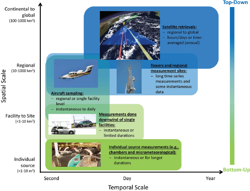
employed. Chamber techniques, vehicle-mounted sensor techniques, and aircraft sampling tend to capture snapshots of emissions over shorter time periods. Some micrometeorological techniques and high-tower monitoring may provide information from days to years. Satellite retrievals that cover regional to global scales may provide instantaneous snapshots or be time averaged to provide longer-term measurements.
This chapter describes global-, continental-, and regional-scale atmospheric methane measurements, along with the models used to estimate emissions from these top-down measurements. Bottom-up approaches are also described, and recent measurement techniques used for specific source categories are reviewed. The strengths and weaknesses of various top-down and bottom-up approaches are summarized in Tables 3.1 and 3.2. These tables do not explicitly address uncertainties; however,
| Technique | Method | Advantages | Disadvantages |
|---|---|---|---|
| Point-source measurements |
|
|
|
| Enclosure (chamber) techniques |
|
|
|
| Technique | Method | Advantages | Disadvantages |
|---|---|---|---|
| Micrometeorological techniques |
|
|
|
| Perimeter facility line measurements |
|
|
|
| Technique | Method | Advantages | Disadvantages |
|---|---|---|---|
| External tracer |
|
|
|
| Inverse dispersion modeling |
|
|
|
| Technique | Method | Advantages | Disadvantages |
|---|---|---|---|
| Facility-scale in situ aircraft measurements |
|
|
|
TABLE 3.2 Top-Down Techniques for Measuring Methane Emissions
| Technique | Method | Advantages | Disadvantages |
|---|---|---|---|
| Remote observatories |
|
|
|
| Towers |
|
|
|
| Aircraft mass balance measurements |
|
|
|
| Aircraft remote sensing measurements |
|
|
|
| Technique | Method | Advantages | Disadvantages |
|---|---|---|---|
| Satellite |
|
|
|
a The sensitivity footprint of an observation at a tower is the region over which emissions can be sensed at that tower. Sensitivity footprints can change with meteorological conditions, and near-field, upwind signals are usually most heavily represented.
NOTE: TROPOMI = TROPOspheric Monitoring Instrument.
uncertainties in top-down and bottom-up methods are addressed in detail later in this chapter and in Chapter 4.
BOTTOM-UP TECHNIQUES FOR MEASURING METHANE EMISSIONS
Bottom-up emission inventories, as discussed in Chapter 2, have historically been developed by multiplying activity data (e.g., numbers of livestock, natural gas operations, landfilled waste) by emission factors (e.g., emissions per head of livestock, emissions per natural gas facility). However, for some anthropogenic sources of methane (e.g., landfills, manure), such simple calculations are generally inappropriate. Emissions from such sources are microbially driven or are subject to significant differences in equipment or operating practices, and as such, they are subjected to large temporal and spatial variability. This requires better temporal and spatial coverage when conducting measurements.
Site-specific research projects have applied multiple field techniques to measure methane emissions. While the nature and sources of activity data vary among sources, many source categories rely on similar methods to measure emissions as the basis for emission factors. In general, the bottom-up techniques described below have application in all source categories discussed in this report. Thus, rather than describe each of these techniques separately for each source, the general methodologies are described first, followed by those more specific to individual source categories.
Overview of Bottom-Up Measurement Methodologies
Methane emissions can be quantified from point sources and area sources using a wide variety of bottom-up techniques, ranging from the direct determination of methane concentration and flow rate at a single leaky valve to aircraft-based mass balance techniques applied to a facility. In between those extremes are
- chamber techniques that use a time series of methane concentrations to determine diffusive soil fluxes at square meter scales or emissions from single or small groups of animals;
- whole-building mass balance approaches to quantify livestock emissions;
- micrometeorological methods to derive emissions from the turbulent transfer of gases over hundreds of square meters at the base of the atmospheric boundary layer; and
- perimeter facility line measurements, inverse dispersion modeling, and external tracer methods to derive atmospheric methane transport rates over square kilometer scales.
Point-Source Measurements
Some emission sources have discrete, well-defined emission points (i.e., valves), and emission rates can be determined directly from the composition and flow rate of the gas at that point. Stack sampling at combustion exhaust points is a common application, but other types of discrete, well-defined emission points also exist. For example, coal mine ventilation systems can release methane through stacks; pneumatic valves and multiple discrete sources in both the petroleum and natural gas supply chains can emit methane as they operate. One approach for measuring point sources is the use of “calibrated bags” where the sample bag, when fully inflated, contains a known volume of gas collected over a known time period. Also, for ruminant animals, enteric methane emissions for individual cows can be measured using an internal tracer technique (Zimmerman, 1993). In other applications for industrial point sources, measurement devices sampling at a known flow rate attempt to capture the entire emission stream—the methane emission rate is calculated by multiplying the sampling rate by the methane concentration minus the background air concentration.
Enclosure (Chamber) Techniques
Emissions of methane from surfaces can be directly determined using small chambers placed on top of the source (e.g., soil surfaces and manure storage surfaces). For static
chambers, diffusive methane emissions are quantified directly from the change in methane concentration over a short time series multiplied by the chamber volume/area ratio (Rolston, 1986). Dynamic chambers (flux gas flowing through a chamber at a known rate) measure emissions based on the difference between the inlet and outlet methane concentration and the flow rate of the flux gas (Eklund, 1992). The chamber approach has been used for quantifying emissions from landfills and above pipelines, water surfaces (using floating chambers) in manure management lagoons, individual or small groups of animals, and multiple other applications. Chambers for surface measurements typically enclose 1 m2 or less and are useful to quantify the variability of emissions; however, they are a labor-intensive technique which can be partly mitigated using automated chamber systems and specialized chambers with volumes >1 m3. Importantly, static chambers can also directly quantify uptake of atmospheric methane by soil methanotrophs with high oxidizing capacities (e.g., negative flux [Bogner et al., 1997] for landfill soils).
Micrometeorological Techniques
If emissions from a source area cannot be enclosed or captured, there are several micrometeorological techniques that can estimate methane emissions using towers with fast-response methane sensors and wind speed/direction sensors, combined with atmospheric transport modeling. Measurements made at a particular site and height represent the conditions of the underlying surface upwind of the sensor. This area of influence is called the “footprint” and is dependent on factors such as measurement height, roughness height, stratification, the standard deviation of the lateral wind component, and wind velocity. Therefore, to accurately assess source emissions, the footprint must cover a large enough area of the source to capture the spatial variability of emissions. The flux gradient technique determines the vertical flux of a gas at a given height as a product of the gas’s turbulent diffusivity and the concentration gradient at that height (Laubach and Kelliher, 2004). The integrated horizontal flux technique depends on a mass budget equation, simplified for two-dimensional flow (Laubach and Kelliher, 2005). A micrometeorological mass balance method can be utilized by measuring all input and output gas emissions within a given volume of air around the source with the emission rate calculated by subtraction of output and input fluxes (Harper et al., 2011; Ryden and McNeill, 1984). The eddy covariance technique calculates fluxes from rapid measurements of the vertical wind speed and gas concentrations (Harper et al., 2011; Prajapati and Santos, 2017). See Harper et al. (2011) for other micrometeorological techniques.
Perimeter Facility Line Measurements
Perimeter facility line measurements are conducted by equipping a site with open-path spectrometers (infrared, tunable diode laser), which measure average methane concentrations per meter distance on the upwind and downwind sides of a site. The emission rate is then estimated by multiplying the difference between upwind and downwind concentrations by the ventilation rate across the site. Some measurement systems use open-path spectrometers with reflectors at multiple elevations to obtain cross sections of the methane plume (e.g., Childers et al., 2001; Goldsmith et al., 2012).
External Tracer
Measurement of methane emissions from area sources (e.g., landfills, livestock housing areas, and natural gas well sites) can also be accomplished by utilizing an external tracer. In this approach a tracer gas not emitted by the facility (often nitrous oxide or acetylene) is released at a known rate at or near the source area of interest. Downwind measurements are made of the tracer and methane, and the methane emission rate is estimated by multiplying the tracer release rate by the concentration ratio of methane to tracer observed downwind (e.g., Dore et al., 2004; Harper et al., 2011; Lamb et al., 1995). The estimated emission rate relies on the assumption that methane and the tracer undergo equivalent atmospheric dispersion between the source and the measurement location. This assumption can break down if some portion of the emissions from a site are buoyant (e.g., partially unburned methane in combustion exhaust) (Vaughn et al., 2017) and the tracers are not similarly buoyant or if the source contains a mixture of buoyant and nonbuoyant tracers. The assumption can also break down if some emissions are released from elevated locations (e.g., from the top of a storage tank) while others are at ground level. To address these issues, some investigators (e.g., Herndon et al., 2013) have used multiple external tracers for a single source measurement, locating one type of tracer release at an elevated release point and other tracer releases near ground level. When colocated, multiple tracers can also be used to provide a quantitative estimate of the extent to which the tracer and the targeted emissions do not undergo equivalent dispersion.
Inverse Dispersion Modeling
Methane emissions from point and area sources can also be determined utilizing inverse dispersion modeling by making downwind measurements of methane alone (without an external tracer), along with measurements of background methane concentration
and wind speed, wind direction, and air turbulence. Those data are then coupled with dispersion modeling to estimate an emission rate. Similar to micrometeorological techniques, in order to accurately assess source emissions, the footprint must cover a large enough area of the source to capture the spatial variability of emissions.
Downwind concentrations can be measured in a variety of ways. One approach is to measure methane concentrations at a consistent height above ground level downwind of the source on a moving platform, often a vehicle. If the vehicle drives along a path that is perpendicular to the wind direction, the horizontal extent of the plume can be determined. Typically, the observed concentrations and their variability across the plume are fitted to a dispersion model to estimate an emission rate (Brantley et al., 2014; Flesch et al., 2005). Because of the high spatial and temporal variability of diffusive emissions from landfill surfaces, generally poor matches are observed between predicted and measured downwind methane concentrations using standard dispersion models. Some investigators have outfitted vehicles with the ability to measure concentrations at multiple heights above ground level, improving the characterization of the plume and the precision of the emission estimate. Other investigators have used techniques that measure an integrated methane concentration in the entire atmospheric column above the vehicle rather than at specified heights (Mellqvist et al., 2016). Downwind concentration measurements can also be made at a stationary point or over a fixed distance using open-path instruments, along with the three-dimensional wind statistics, and fitted to a dispersion model to estimate an emission rate (Flesch et al., 2005; Leytem et al., 2011).
The accuracy of this method depends on the situation in which it is used. For example, several validation studies using a backward Lagrangian stochastic inverse dispersion technique to measure emissions from livestock report errors of less than 20 percent, likely because these emissions are relatively uniform (e.g., Gao et al., 2010; McGinn et al., 2009; Ro et al., 2013). However, for measuring methane emissions from petroleum and natural gas, which tend to be more variable, errors may be much higher. A recent analysis of emission estimates based on dispersion modeling downwind reports error bounds of +117/−46 percent (Robertson et al., 2017).
Facility-Scale In Situ Aircraft Measurements
Aircraft-based measurements can be used to estimate emissions from individual facilities (e.g., an animal feeding operation, a landfill, or a natural gas processing facility). A typical approach is to fly concentric closed flight paths at multiple altitudes around a source while continuously measuring methane concentrations, wind speed, and wind
direction. Emission rates are estimated using a mass balance approach; the concentration differences between the upwind and downwind portions of the flight paths are multiplied by the ventilation rate for the volume enclosed by the flight paths to arrive at the emission estimate (e.g., Conley et al., 2017; Gvakharia et al., 2017). These techniques have been applied to a variety of methane sources in urban areas (e.g., Cambaliza et al., 2015; Mehrotra et al., 2017). This approach is at a relatively early stage compared to other methods (e.g., tracers), and there are several limitations that need to considered. For example, facility aircraft measurements tend to be successful only under restricted conditions, when there are no confounding sources close to the facility and when aircraft can fly nearly to the bottom of the emission plume. In addition, this approach can only detect emissions that are encountered at flight elevations at the flight radial distance. It is uncertain that the extrapolation from the bottom flight level to the ground is robust for a close-to-ground emission (e.g., a leaking blowdown vent).
Bottom-Up Techniques for Measuring Methane Emissions from Major Sources
Agriculture Sector
There are two sources of methane emissions from livestock: enteric fermentation (predominantly in the digestive tract of ruminant animals) and manure management (methane produced by methanogenesis during manure storage). For some ruminant production systems (e.g., beef or dairy cattle on pasture), enteric fermentation is by far the main source of methane emissions. In ruminant production systems in which manure is handled as liquid (e.g., flush dairy barns, where manure is flushed from the barn with water), methane emissions from manure management can be as high as or even higher than emissions from enteric emissions. For nonruminant production systems (e.g., swine, poultry), methane generated from manure storage is the main source of methane emissions. Methane emissions from livestock are microbially driven and therefore can have large spatial and temporal variability, because microbial activity is governed by the substrate available as well as other conditions. Therefore, care must be taken to ensure that temporal, spatial, and animal (enteric) variability in emissions is captured in order to accurately portray emissions from any given source category.
Enteric Methane
The term “enteric methane” refers to methane produced by microbial fermentation-related activities in the gastrointestinal tract of ruminant or nonruminant animals (for more information on these processes, see Hristov et al., 2013). Ruminant animals are
the largest contributor to methane emissions from agriculture. Nonruminant farm animals, however, also emit methane through fermentative activities in their hindgut.
Enteric methane can be emitted by ruminants through eructation, expiration, or flatulence. Earlier (Murray et al., 1976) and more recent (Muñoz et al., 2012) data have unequivocally shown minimal contribution of methane (2-3 percent) emitted through flatulence, compared with methane emitted through expiration (exhaling) or eructation (belching). A significant portion of methane produced in the rumen, the largest organ of the digestive tract of the ruminant animal, is absorbed into the bloodstream (12 percent in a study by Reynolds et al., 2013). Most of this methane, however, is exhaled through the lungs (Ricci et al., 2014).
Methods for measuring enteric methane from livestock include enclosure chambers, tracer techniques, “sniffer” techniques, and handheld laser methane detectors.1 The “gold standard” for measuring enteric methane emissions from farm animals (ruminants and nonruminants) is the respiration chamber. The main principles of dynamic respiration chambers are to measure incoming and exhaust airflows, concentration of gases of interest in that air, and initial and final gas concentrations in the chamber. A detailed discussion on the design and operation of respiration chambers was provided in the Technical Manual on Respiration Chamber Designs, published by the Global Research Alliance (Pinares-Patiño and Waghorn, 2012). Animals are usually placed in chambers for several days (recommendations are for at least 3 days), during which they are fed and milked (if lactating), and manure is removed from the chamber. The animals have to acclimatize to the chamber environment before measurements take place. The main advantage of respiration chambers is that (1) they are accurate when properly calibrated and operated, (2) all methane emissions, including from the anus, are captured, and (3) measurements take place continuously over several days, accounting for diurnal variation in methane emissions. The results of a recent ring test of respiration chambers in the United Kingdom demonstrated the importance of calibration for the accuracy and precision of respiration chambers (Gardiner et al., 2015). The drawbacks of respiration chambers are that (1) animals are placed in an “unnatural” environment, which in many cases results in stress and decreased feed intake and/or milk production; (2) chambers cannot be used to measure emissions from a large number of large animals concurrently (which is important for genetic selection of low-methane emitters); and (3) they are expensive and require extensive training and operational skills.
___________________
1 A comprehensive review of enteric methane measurement techniques was recently published by an international team of scientists (Hammond et al., 2016) as part of the Global Network project (http://animalscience.psu.edu/fnn/current-research/global-network-for-enteric-methane-mitigation). Materials from the Hammond et al. (2016) review were extensively used in the preparation of this section.
While chamber systems can be utilized to measure emissions from ruminants and nonruminants, there are a variety of other techniques available to measure enteric methane emissions from ruminant animals. A widely used technique is the sulfur hexafluoride (SF6) tracer method (Figure 3.2). Originally developed by Zimmerman (1993) and first used by Johnson et al. (1994), the method was recently modified and improved by Deighton et al. (2014). The technique is based on using a tracer gas, SF6, which is continuously released at a known rate from a permeation tube placed in the reticulum (one of the compartments of the complex ruminant stomach) and mixed with rumen gases. Eructated and expired gas is continuously sampled around the nostrils of the animal into an evacuated container and the gas is analyzed for SF6 and methane. The ratio of the two gases and the SF6 release rate are used to calculate the methane emission rate. The technique is less costly compared with the investment to build and operate respiration chambers, and has been widely used by research groups around the globe. Variability with the SF6 technique has been notoriously high (Clark,
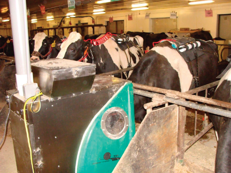
2010; Pinares-Patiño and Clark, 2008; Pinares-Patiño et al., 2010), but the modifications by Deighton et al. (2014) addressed the most important sources of error, and the modified technique produces methane measurements with accuracy similar to measurements using respiration chambers. Unlike chambers, the SF6 technique can be used to measure methane emissions from a large number of animals and in their natural environment. The technique does not account for methane generated in the hindgut and excreted through the rectum. Detailed guidelines for using the technique have been published by Berndt et al. (2014).
Several important conditions have to be met to reduce variability in the methane measurement data when the SF6 technique is used. These include (1) high release rate of SF6 from the permeation tube, (2) at least five consecutive measurement days, and (3) low concentrations of SF6 and methane in background air (i.e., using the technique in enclosed barns is not recommended, unless there is adequate ventilation throughout the measurement period; Hristov et al., 2016). When these conditions are met, the SF6 tracer technique can produce accurate methane emission data from a large group of animals.
More recently, an automated head chamber system, GreenFeed® (GF), was developed for spot sampling of exhaled and eructated gases (Zimmerman and Zimmerman, 2012). Comparisons with respiration chambers or SF6 have established that when properly used, GF is a reliable technique for measuring enteric methane emissions from ruminant animals (Dorich et al., 2015; Hammond et al., 2015; Hristov et al., 2016). Similar to the SF6 technique, the GF system can be used to monitor methane emissions from a group of animals in their natural environment. The technique is based on attracting the animal to the GF head chamber and keeping it there for at least 5 minutes at each sampling event while eructated and exhaled gases are captured and directed to gas sensors.
An important prerequisite for using the GF system is that all animals visit the unit at all times of the day and night. Methane emissions have a clear diurnal pattern, related to feed intake (usually lower at night) and therefore, for accurate daily emission estimates, animal visits have to be spread out over a 24-hour feeding cycle. Best results with the GF system are obtained when the number and timing of animal visits are controlled by the investigator, which is easily achievable in a tie-stall barn situation (Branco et al., 2015; Hristov et al., 2015b), or measurements have to take place over a prolonged period (3-5 weeks, depending on the study objectives; Renand and Maupetit, 2016). Studies conducted in pasture conditions may need longer time to achieve the number of required visits than those conducted in confinement. Recommended GF calibration and background gas collection procedures have to be strictly
adhered to (Hristov et al., 2015a). Similar to the SF6 technique, GF cannot measure methane excreted through the rectum.
Another direct technique with limited application is the ventilated hood chamber or box (Kebreab, 2015), which is a polycarbonate chamber enclosing the head of the animal, allowing continuous collection and analysis of eructated and exhaled gases. A neck sleeve allows the animal to lie down and eat while measurements take place. The chamber is under constant vacuum, and incoming and exhaust air is analyzed for methane concentration. Detailed description of such a chamber can be found in Place et al. (2011). Drawbacks of this technique are that (1) hood chambers require a significant investment, (2) the animals must be extensively trained to minimize stress during the experiment, (3) the animals’ feed intake will likely decrease while fed in the chamber, and (4) the technique is not suitable for measuring methane emissions from a large group of animals.
Indirect approaches have been proposed and used to measure enteric methane emissions from livestock. One approach uses estimated carbon dioxide emissions and measured carbon dioxide/methane ratio in exhaled air to estimate methane emissions (Madsen et al., 2010). This method is based on the fact that most of the carbon dioxide is produced by intermediary metabolism of the animal and can be predicted. If total carbon dioxide production and the carbon dioxide/methane ratio are known, total methane production can be calculated. Hellwing et al. (2013) compared the carbon dioxide method to respiration chambers and found a significant underestimation of emissions by the carbon dioxide method. Changes in digestive and metabolic activities at the same level of feed intake, differences in feed efficiency, and variation in rumen fermentation can influence the amount of carbon dioxide produced by the animal and thus affect the predicted methane emissions (Huhtanen et al., 2015).
Another indirect method proposed by Garnsworthy et al. (2012) relies on estimating methane emissions during an eructation event and the frequency of eructation during a measurement period. Gas samples are collected from the air in the feed manager of an automated milking system when the animal is milked. The attractiveness of this approach (also referred to as the “sniffer” method) is that emissions can be measured in on-farm conditions and on a large number of animals. This method does not account for methane exhaled through the lungs. The authors have reported a good correlation between the “sniffer” and chamber measurements for the same animals (Bell et al., 2014; Garnsworthy et al., 2012). However, even small changes in head position can result in large differences in gas concentration (Huhtanen et al., 2015). In two experiments with lactating cows, Huhtanen et al. (2015) found larger variability with the “sniffer” method and no relationship to emissions measured using the GF system.
Another recent study also concluded that the capability of the “sniffer” method to adequately measure and rank methane emission rates among dairy cows is highly uncertain and requires further investigation into the sources of variation (Wu et al., 2017).
A technique similar to the “sniffer” method utilizes a laser methane detector to measure methane concentration in the air between the laser device and the animal (usually 1-3 m). The method allows methane measurements in on-farm conditions and from a large number of animals; however, comparative studies found a positive but weak relationship between the laser method and chamber measurements (Chagunda et al., 2013; Ricci et al., 2014). Environmental factors such as temperature, wind velocity (particularly important for grazing conditions), and humidity can affect the accuracy of the measurements).
Accurate techniques for measuring enteric methane emissions from livestock are available. Although some of these techniques can measure methane emissions from a significant number of animals (about 20 per piece of equipment) in their natural environment, they are inappropriate for screening of animals at the population level for selection of low-methane emitters.
Manure Management
Manure management systems may include open areas for drying, stacking, or composting manures as well as liquid/slurry storage systems consisting of separation basins, mechanical separators, tanks, pits, and lagoons. Depending on the type of system present at a facility, the measurement techniques for estimating emissions from these sources will vary. For enclosed barns that are mechanically ventilated, emission rates can be determined by mass balance methods. For open housing systems, measurement techniques can include mass balance, external tracer techniques, inverse dispersion modeling, and micrometeorology techniques. Measuring methane emissions from manure storage is typically accomplished using external tracer techniques, inverse dispersion modeling, micrometeorology techniques, or chambers.
Facility-level emissions will include emissions originating from both enteric emissions and manure management, while manure management emissions aim to target those emissions originating from manure in housing as well as manure handling and storage areas. Facility-level emissions can be determined with a variety of larger-scale measurement platforms, such as airplane sensors (see earlier section in this chapter on airplane measurements) or inverse dispersion modeling. Information at this scale can provide overall emission rates for a given facility but are not able to discern the
source of emissions from within a facility. For airplane sensors, because of the expense of flight campaigns and the dependency on favorable weather conditions, data will likely only cover small temporal scales and in many instances only provide information during midday hours when emissions are likely to be greatest from a facility. Therefore, important diurnal and seasonal changes affecting overall annual emissions may not be captured. While inverse dispersion techniques can capture the temporal variability in emissions, individual sources within the facility may not be discernable.
At the component level (e.g., housing, manure handling, and manure storage), a variety of techniques can be utilized to determine emissions. Mass balance techniques can be used to measure emissions from enclosed barns or other areas (manure storage) that are mechanically ventilated. This technique consists of measuring the gas concentration continuously over time at the barn inlet and outlet along with the ventilation flow rate (Amon et al., 2001; Kinsman et al., 1995). The measured emissions will include both enteric (for barns) and manure. This measurement technique works well as long as the monitoring equipment is kept well calibrated for measuring the ventilation rate. Measuring emissions from naturally ventilated livestock buildings presents a greater challenge because it is difficult to determine the ventilation rate. In these instances the ventilation rates can be estimated using a carbon dioxide balance or tracer gas technique. The carbon dioxide balance technique utilizes carbon dioxide formed by animal respiration as a natural tracer gas with the ventilation rate estimated by calculating the mass balance of carbon dioxide flow (Pedersen et al., 1998). Alternatively, a tracer gas (i.e., 85Kr or others) can be distributed inside the building and used to estimate ventilation rate (Marik and Levin, 1996; Samer et al., 2011). Measurement of methane within the barn, along with the estimated ventilation rates, is used to calculate the overall emission rate (Fiedler and Muller, 2011; Snell et al., 2003). These techniques can provide good estimates of emissions from housing areas; however, they will not directly allow estimation of the contribution of enteric versus manure emissions. They can also be employed over longer time periods that capture the temporal variability of emissions, providing better long-term emission estimates.
Additional methods can be employed that do not rely on calculating or estimating ventilation rates and can be applicable to open source areas (dry lots, pasture, manure storage areas, etc.). These include external tracers (Dore et al., 2004; Harper et al., 2011), dispersion models (Flesch et al., 2005; Harper et al., 2011), flux gradient, integrated horizontal flux, micrometeorological mass balance, and eddy covariance (Harper et al., 2011). All of these open-air techniques have the advantage of being able to measure methane emissions from a source area without disturbing animals or altering ambient conditions. Because they measure the emissions from the entire source area (or large portions of it), spatial variability of emissions is also accounted for. Most of these tech-
niques are also easily employed over longer time periods, which provide coverage of temporal variability, enabling more accurate prediction of longer-term emissions.
Techniques available for targeted analysis of specific surfaces include the use of chambers (Amon et al., 2001; Ellis et al., 2001; Misselbrook et al., 2001). Although these techniques can provide emission estimates for a given source area, there are several potential drawbacks to consider. Because of the small size of most chambers, the ability to capture the spatial variability of emissions from the source area may be difficult. During measurement, the chamber itself can alter the environment (e.g., temperature and airflow) of the source area, which may affect emissions. Capturing the temporal variation in emissions can also be difficult because chambers may not be able to be deployed for long periods of time because the disturbance to the ambient atmospheric conditions is too great. However, there have been some automated and floating chambers designed to work over long periods to overcome the challenge of capturing temporal changes in emissions.
Because of the temporal and spatial variability of emissions from livestock housing and manure management, measurements and monitoring need to occur over longer periods of time that cover both the daily and seasonal variations in emissions in order to accurately reflect annual emissions.
Petroleum and Natural Gas Systems
Methane emissions from petroleum and natural gas supply chain sources reported in national inventories include sources from the wellhead to the point of use of the fuel, but they do not include emissions associated with end use (e.g., unburned methane from electricity power generation). The emission sources are varied, as are the activity data and emission measurement approaches. In addition, in the petroleum and gas category, activity and emission factor data collection activities are linked. For example, if measurements of emissions are used to develop average emission factors for an entire population of sources (e.g., all pneumatic controllers used at natural gas wells), then the activity data are simply a count of the number of sources (e.g., the total number of controllers). In contrast, if measurements identify that emissions vary across subpopulations (e.g., pneumatic controllers of different designs, intended to have different emission rates) then emission and activity data would either need to be collected on multiple subpopulations or sampling would need to be done across all subpopulation categories in such a manner that each subpopulation is proportionally represented in the sample. Both approaches can be difficult to implement. Sub-populations may not be sufficiently defined prior to data collection, and randomized
sampling across subpopulations may be impossible due to expense, study extent (e.g., geographic extent of study region), or restricted access.
For each emission category, there are large numbers of sources to account for and considerable spatial and temporal variability in methane emissions both within and across category and component types. In the United States, there are currently over 600 gas processing plants and over one million pneumatic devices in combined petroleum and natural gas systems. Within each of these categories, a variety of subcategories of sources may exist with variability in emissions among the subcategories. For example, gathering and processing facilities can process from <1 to about 1,000 metric tons (or 0.001 Tg) of gas per hour, and emission rates can vary as a result. However, even among plants of equal size, Marchese et al. (2015) and Mitchell et al. (2015) found that normalized emissions (emissions as a percentage of natural gas throughput) ranged from less than 0.1 percent to more than 10 percent. Within specific equipment categories, such as pneumatic devices, there are also multiple potential emission subcategories, based on the method of operation of the device (for pneumatics, low bleed, high bleed, intermittent), as well as the type of service in which they are used (for pneumatics, plunger control, separator level control, emergency shutdown, and many others). Allen et al. (2015a) found that emissions per controller varied by more than an order of magnitude between controllers in different types of service (e.g., separator level control versus controllers on process heaters). Thus, while activity data such as numbers of gas processing plants are generally available for estimating methane emissions from sources in the petroleum and gas supply chains, it is not clear that the level of detail in the activity data of the inventory is sufficient for accurately estimating annual methane emissions.
Measurement Studies to Update Emission Factors and Activity Data
Prior to 2013, many of the emission factors that were used in developing methane emission inventories for petroleum and natural gas systems relied on a comprehensive study by the Gas Research Institute and the U.S. Environmental Protection Agency (EPA), conducted in the 1990s (Harrison et al., 1996). Since 2013, however, a number of studies have reported new emission factor data for petroleum and natural gas. Many of these recent studies were coordinated by the Environmental Defense Fund (EDF) and companies owning and operating assets across the natural gas value chain2 from production segment to distribution. In addition, the U.S. Department of Energy (DOE)
___________________
2 The major sectors or operational components of the petroleum and natural gas industry include exploration and extraction, storing, marketing and transporting, and refining and processing.
has funded multiple methane measurement projects.3 Measurements in these studies were conducted by independent, primarily university-based researchers, generally overseen by independent advisory committees and in some cases with industry co-sponsors. Sources on which data have been collected include well completions, pneumatic controllers, pneumatic pumps, leaks, liquid unloadings, flares, gathering operations, gas processing facilities, transmission facilities, and pipelines. The measurement techniques used in EDF-coordinated and DOE studies and other recent emission studies have employed most of the methods described in Table 3.1.
Because the EPA has incorporated some of this new information into Greenhouse Gas Inventory (GHGI) development and new regulations have been finalized that have reduced emissions from specific types of equipment and operations, large changes in the estimated inventories of methane from petroleum and natural gas systems have occurred. For example, in Marchese et al. (2015), Zimmerle et al. (2015), and Lamb et al. (2015), results were employed to update methane emissions from the gathering and boosting, transmission, and distribution segments, respectively (see Chapter 2). In some cases, the changes in emissions are the result of changes in regulations and operating practices. For example, in the 2011 GHGI (released in 2013), emissions from natural gas well completions, summed over the duration of the completions, were estimated to total 0.65 Tg from a total of 8,077 well completions, resulting in average methane emissions per well completion of 81 metric tons (or 0.000081 Tg). With the promulgation of New Source Performance Standards, requiring reduced emission completions for natural gas wells beginning in 2012, methane emissions were reduced by approximately 99 percent compared to an uncontrolled well completion for a limited number of wells on which completion emissions have been measured (Allen et al., 2013). In the 2017 GHGI, well completion emissions, including well workovers with hydraulic fracturing, were estimated to be about 0.03 Tg (an average of 2 metric tons per well).
Other emission inventory changes have been due largely to changes in activity counts. For example, in the 2011 GHGI for natural gas, an activity count for pneumatic controllers averaging one controller per well was used. A series of field studies, together with data on average controller counts per well collected through the Greenhouse Gas Reporting Program (GHGRP), have led to a revision of the activity data for pneumatic controllers. The 2015 GHGI reports an average of 1.9 controllers per well (EPA, 2017b).
___________________
3 See https://energy.gov/sites/prod/files/2016/08/f33/Methane%20Emissions.pdf and https://www.energy.gov/under-secretary-science-and-energy/articles/doe-announces-13-million-quantify-andmitigate-methane.
These updates, while important in improving the accuracy of emissions documented in the GHGI, can lead to fluctuations in the GHGI from year to year (Figure 2.9).
A common element in many of the recent methane emission studies on natural gas is the presence of high-emitting sources, that is, a small number of sites or equipment that contribute a disproportionately high fraction of the cumulative total emissions recorded (Box 2.2). Some measurements of high emissions may be due to the size of the facility. For example, a natural gas processing plant with a capacity of greater than 1 metric ton (or 0.000001 Tg) per hour might be expected to have greater emissions than a plant with a capacity of less than 1 metric ton per hour; however, even when emissions are normalized by gas throughput or gas produced, a small number of observations with high normalized emissions have been identified. As documented in Table 3.3, these high-emitting sources are found in many studies of various source categories, including many studies with site access and cooperation of industry participants.
A meta-analysis4 by Brandt et al. (2016) of about 15,000 measurements from 18 studies (including many cited in Table 3.3) found that methane emissions from natural gas systems follow an extreme distribution, resulting in a small fraction of observed emissions accounting for a vast majority of the emissions from the population sampled. Schwietzke et al. (2017) attribute observed known high-level emissions to episodic events in manual liquid unloadings. Compliance inspections have observed potential design constraints and operational issues that may result in chronic high emissions.5 Stochastic events arise from malfunctions that could result in high-emission events and are difficult to predict.
For petroleum and natural gas, factors that cause certain subpopulations to become high emitters are not well known. Research is needed to gain a mechanistic understanding of high-emitting sources and establish appropriate estimation methods. Conducting campaigns in coordination with owners and operators of the facilities within the regions would help ensure the availability of contemporaneous information concerning operations.
___________________
4 “Meta-analysis” is a statistical analysis that combines the results of multiple scientific studies.
5 See https://www.epa.gov/enforcement/noble-energy-inc-settlement#violations, https://www.epa.gov/sites/production/files/2015-04/documents/noble-cd.pdf, and https://www.courthousenews.com/wpcontent/uploads/2017/10/pdc-cd.pdf.
TABLE 3.3 A Sample of Bottom-Up Measurement Studies in the Natural Gas Supply Chain
| Geographic Region Sampled | Devices Sampled | Emission Factor | High-Emitting Sources | Reference |
|---|---|---|---|---|
| Natural Gas Production Sites | ||||
| U.S. national sample of natural gas sites | Well completions, unloadings, leaks, pneumatic pumps, and controllers | Emission factors for leaks and pneumatic controllers higher than in EPA GHGI; emission factors for well completions lower than in GHGI. | Observed for unloadings, pneumatic controllers. | Allen et al., 2013 |
| U.S. national sample of primarily natural gas sites | Pneumatic controllers | Emissions per controller 17% higher than average in GHGI (5.5 scfh [0.2 scmh] whole gas, 4.9 scfh [0.1 scmh] methane). | 19% of controllers accounted for 95% of national emissions from pneumatic controllers. | Allen et al., 2015a |
| Oklahoma petroleum and natural gas sites | Pneumatic controllers | Emissions averaged 1.05 scfh (0.03 scmh) whole gas for all devices. | 3.5% of controllers accounted for 73% of controller emissions. | Gibbs, 2015 |
| Utah petroleum and natural gas sites | Pneumatic controllers | Emissions averaged 0.36 scfh (0.01 scmh) whole gas for all devices. | Majority of emissions came from 14 of the 80 controllers; 11 of the 14 high-emitting controllers were malfunctioning. | Thoma et al., 2017 |
| U.S. national sample of natural gas sites | Liquid unloadings | Average emissions equivalent to those reported in EPA GHGI. | 2-3% of wells account for more than half of national unloading emissions. | Allen et al., 2015b |
| Geographic Region Sampled | Devices Sampled | Emission Factor | High-Emitting Sources | Reference |
|---|---|---|---|---|
| Marcellus Shale natural gas site | Flare | Very high combustion efficiencies (>99.5%) for a single well completion flare; bottom-up inventories generally assume 98% efficiency. | A single flare measured had intermittent high emissions. | Allen et al., 2013 |
| Marcellus Shale, Bakken Shale petroleum and natural gas sites | Flares | All flares were >99.80% efficient at the 25% quartile; bottom-up inventories generally assume 98% efficiency. | No high emitters detected | Caulton et al., 2014a |
| Bakken primarily petroleum sites | Flares | 37 production flares in the Bakken had a median destruction efficiency of 97%. | Some flares with destruction efficiency <80%. | Gvakharia et al., 2017 |
| Natural Gas Gathering and Processing Operations | ||||
| U.S. national sample of natural gas sites | Downwind sampling of sites | Emissions averaged 0.20% of throughput for gathering facilities and 0.075% of throughput for processing facilities. | Some gathering facilities had emissions that were in excess of 10% of gas throughput and 30% of gathering facilities contributed 80% of the total emissions; all processing facilities had emissions <1% of throughput. | Marchese et al., 2015; Mitchell et al., 2015 |
| Geographic Region Sampled | Devices Sampled | Emission Factor | High-Emitting Sources | Reference |
|---|---|---|---|---|
| Natural Gas Transmission and Storage | ||||
| U.S. national sample | Downwind sampling of sites, with onsite measurements and emission estimates | Emission factors both higher and lower than inventory factors observed; largest emission factor from open-ended lines (measurement factor of 5 greater than GHGRP emission factor). | Highest-emitting 10% of sites (including two high-emitting sources) contributed 50% of aggregate methane emissions. | Subramanian et al., 2015; Zimmerle et al., 2015 |
| Natural Gas Distribution, Metering, and Regulating (M&R) | ||||
| Thirteen urban distribution systems | Direct sampling of emissions | Emissions of 0.10% to 0.22% of the methane delivered, equivalent to 36% to 70% less than the 2011 EPA GHGI; emission factors reported for multiple types of pipes and for M&R facilities, multiple pressures. | Large reductions in emissions from high-emitting facilities, compared to measurements made in early 1990s (Harrison et al., 1996). | Lamb et al., 2015 |
| Multiple cities | Downwind sampling | Emission rates were empirically correlated with maximum concentrations measured by an instrumented vehicle, using calibration experiments. | Urban areas with corrosion-prone distribution lines leaked ~25-fold more methane than cities with more modern pipeline materials. | von Fischer et al., 2017 |
| Boston | Centralized monitors on tall buildings | 2.7 ± 0.6% of natural gas use, also including urban end-use emissions. | Not applicable. | McKain et al., 2015 |
SOURCE: Adapted and expanded from Allen, 2016.
Landfills
In contrast to other anthropogenic sources of methane, simple (activity data multiplied by emission factor) calculations are generally inappropriate for estimating landfill methane emissions because of the complexity of soil-gas transport and oxidation processes in landfill cover soils (see also Chapter 2). The two major drivers for landfill methane emissions at specific sites are seasonal climate and site engineering/operational practices, including (1) the thickness and physical characteristics of cover materials and (2) the extent of engineered biogas extraction (Gebert et al., 2011; Goldsmith et al., 2012; Scheutz et al., 2009; Spokas et al., 2011, 2015). Major field campaigns and process-based model development have occurred in recent years, providing important new results quantifying methane emissions from landfills and providing improved inventory approaches. Also, landfills must presently comply with minimum cover requirements, standards for biogas management, required biogas recovery at larger sites, quarterly surface scans for elevated methane concentrations, and other operational guidelines under both Subtitle D of the Resource Conservation and Recovery Act and Clean Air Act mandates. These requirements vary somewhat among states to conform with regional differences in landfill practices as well as state requirements that may be stricter than federal minimum standards.
Landfill emissions are challenging to quantify because of high spatial and temporal variability (Scheutz et al., 2009; Spokas et al., 2011, and references cited therein), including drastically different emission signatures from adjacent cover soils (daily, intermediate, final) and temporal variability in soil oxidation. Both gaseous transport and oxidation rates are dependent on dynamic changes in soil temperature and moisture resulting from local weather fluctuations, as well as longer-term climate trends (Spokas et al., 2011). Laboratory study of cover soils conducted over a wide range of temperature and moisture conditions indicates that optimum oxidation rates occur at soil temperatures around 35°C and soil moisture potentials near the water-holding capacity (about 10 kPa; Spokas and Bogner, 2011).
In general, the highest average emission flux (normalized to grams of methane per square meter per day) has been associated with the working face/daily cover areas at sites in humid subtropical climates, while lower emissions are associated with thicker final cover soils (Babillote, 2011; Goldsmith et al., 2012). At many sites, however, it can be demonstrated that the intermediate cover areas emit the largest percentage of total emissions due to their large surface area and thinner cover soils (than final covers) (Spokas et al., 2015). Importantly, the presence or absence of engineered biogas recovery under a particular cover area (either vertical wells or horizontal collectors installed concurrently with filling) determines the “base of cover” soil gas methane
concentration and the driving force for diffusive methane emissions to the atmosphere (Spokas et al., 2011).
Multiple field campaigns during the last two decades have greatly improved understanding of landfill methane emission processes at U.S. sites. Moreover, during the last decade, a process-based model (CALMIM, California Landfill Methane Inventory Model) has been developed and field validated to provide a predictive framework for site-specific climate and cover-specific gaseous transport and oxidation processes over a typical annual cycle (Spokas et al., 2011, 2015). At present, this model has not been incorporated into the U.S. GHGI or GHGRP.
Field Measurements and Modeling
Field measurement techniques for landfills range from square meter to square kilometer scales, including chambers, tracer techniques, micrometeorological approaches, vertical radial plume mapping (VRPM), and aircraft mass balance approaches, as discussed below and previously summarized in Table 3.3.
In general, the parallel use of labor-intensive static chambers deployed at ground level in combination with other techniques discussed below is desirable because chambers (1) can be deployed at any hour of the day or night, (2) constitute a direct measurement technique that does not require atmospheric modeling to infer methane mass flux rates, and (3) can quantify the spatial and temporal variability of emissions across a given cover type. Moreover, static chambers can also quantify “negative” emissions (e.g., uptake of atmospheric methane), which can occur in landfill cover soils with high seasonal oxidation capacities (Bogner et al., 1997, 2011; Scheutz et al., 2009, and references cited therein). In addition, soil gas probes used in parallel with static chambers are useful to characterize in situ molecular and isotopic profiles for improved understanding of methane generation, transport, and oxidation dynamics. Innovative techniques used in landfill settings include double tracer techniques deployed at field scale (Scheutz et al., 2011), soil gas “push-pull” tests to quantify oxidation (Streese-Kleeberg et al., 2011), and refinements of micrometeorological approaches to better capture atmospheric transport dynamics at landfills (Taylor et al., 2016).
Landfill methane recovered directly from the buried (anaerobic) waste has a relatively constant isotopic signature for carbon (δ13C of around −60%0); hence, techniques that quantify the change in δ13C for oxidized landfill methane in chambers, probes, or downwind plumes can directly quantify the extent of oxidation at field scale. Research results indicate that seasonal oxidation is highly variable and underestimated by the current Intergovernmental Panel on Climate Change (IPCC, 2006) default of 10 percent,
with average values in the 30 percent range (Chanton and Liptay, 2000; Chanton et al., 2009, 2011; Liptay et al., 1998; see also Chapter 2). Isotopic fingerprinting using the δ13C of methane and carbon dioxide has also been used to verify seasonal methane production in a landfill cover soil (Bogner et al., 2011). In general, the δ13C of emitted landfill methane can range from −60%0 (negligible oxidation) to −30%0 due to oxidation (Bogner et al., 1997, 2011), generally negating its value for fingerprinting landfill methane in atmospheric studies. It should also be noted that all landfills typically have a combination of operational areas with thin daily cover soils, recently completed areas with thicker intermediate cover that will be subject to future vertical expansion, and areas at final grade with very thick or geomembrane composite permitted final covers. This complexity further exacerbates use of atmospheric carbon isotopes to fingerprint landfill methane.
Using modern sequencing techniques, new insights into methane-oxidizing landfill soil microbial communities are also emerging. For example, Henneberger et al. (2015) assessed spatial and temporal changes in methane-oxidizing communities in a landfill cover soil using field-based measurements of oxidation activity, stable-isotope probing of polar lipid-derived fatty acids, and microarray analysis of pmoA genes and transcripts. Because of variable environmental conditions (temperature, moisture, soil processes), active microbial communities were highly diverse with distinct spatial and seasonal clustering, including the concurrent presence of atmospheric methane oxidizers.
Recent multiple-landfill U.S. field campaigns have relied on diverse bottom-up field techniques to quantify site-level landfill methane emissions and oxidation, thus providing important insights into the strengths and weaknesses of various methods. For example, a comparative study of methane emissions from two adjacent Wisconsin landfills using five methods (Babillote, 2011) included (1) tracer correlation using N2O, (2) an optical remote sensing method (VRPM), (3) static chambers with stable C isotopes to quantify soil oxidation, (4) an eddy covariance micrometeorological method, and (5) differential absorption Lidar (DiAL). Results indicated that the tracer method had minimum error and lowest variability; however, the VRPM, DiAL, and tracer results were all within the same order of magnitude. Moreover, using the DiAL method, working area emissions could be shown to be reduced approximately 50 percent at the end of the working day following the placement of daily cover. Complementary data on methane oxidation using a stable carbon isotopic method (Chanton and Liptay, 2000; Liptay et al., 1998) ranged from 7 to 25 percent for daily covers and from 15 to 45 percent for intermediate covers, with differences attributable both to variable cover thickness and decreased methane loading to the base of the cover due to the biogas extraction system. These results support the continued use of multiple techniques in
parallel to quantify the variability of emissions for individual cover materials at various temporal scales. Goldsmith et al. (2012) subsequently reported on use of a tunable diode laser spectrometer for path-integrated methane within a VRPM based on the EPA OTM-10 method at a large number of U.S. sites. Conclusions emphasized two important challenges with the routine use of VRPM for landfill applications: the topographic irregularities typical of landfill sites and the need for improved quantification of the area contributing to the calculated flux (Abichou et al., 2010; Goldsmith et al., 2012; Thoma et al., 2010).
Recently, joint efforts between the waste industry and the EPA have focused on developing a standardized field methodology for “whole-landfill” emissions with the goal of certification by the EPA as an other test method. This has included the development and application of a tracer correlation method using a C2H2 tracer with the Piccaro cavity ring-down spectrometer (Foster-Wittig et al., 2015). Quantitative acceptance criteria were developed to screen data resulting from insufficiently advected plume transport or poor tracer correlations. The high-emitting sites had total emissions greater than 6,000 g methane min–1. More recently, measured emissions during a 3-year period at a newly opened landfill using the tracer correlation technique discussed above were compared by de la Cruz et al. (2016) to various methane generation and emission models. Their study concluded that IPCC (2006) and similar standard landfill methane generation-based models overestimated emissions by factors ranging from 4 to 31. It is not appropriate, however, to extrapolate these site-specific multipliers to other sites or to the national total due to site-specific differences in operational practices and climate. As previously discussed in Chapter 2, there are fundamental problems with the current inventory methodology, including a lack of systematic field validation for emissions as well as a lack of systematic correspondence with independent field measurements.
During the last decade, a new process-based model (CALMIM) has been developed and field validated for use in quantifying “whole-landfill” methane emissions over an annual cycle. The model provides improved site-specific estimates as the sum of cover-specific methane emissions with and without oxidation for 10-min time steps and 2.5-cm depth increments over a typical annual cycle (using embedded U.S. Department of Agriculture models for average 30-year weather data with 0.5° × 0.5° latitude/longitude reliability). Moreover, CALMIM has utility for other research and engineering applications when used with local annual weather data to examine annual emission trends or assess emissions from proposed alternative cover materials, or when paired with climate projections (e.g., CMIP5) to estimate future emissions (Bogner et al., 2011, 2014; Spokas and Bogner, 2011; Spokas et al., 2011, 2015). This JAVA tool directly models diffusive emissions inclusive of soil oxidation, without any linkage to a theoretical methane generation model
(e.g., IPCC, 2006). To facilitate model use for future inventories, inputs are limited to site latitude/longitude, waste footprint area, cover soil areas, thickness and physical properties of each layered cover soil, and percentage of cover area with underlying biogas recovery.
International field validation for CALMIM included a direct comparison of results to independent field measurements derived from a wide variety of techniques for 40 cover materials at 29 landfill sites on 6 continents (e.g. Bogner et al., 2011, 2014; Goldsmith et al., 2012; Spokas et al., 2011, 2015). Overall, model comparisons to field measurements resulted in a d index of 0.765 using site-specific data (Willmott index of agreement; Willmott, 1981), a Pearson r value > |0.8| for modeled versus measured comparisons at 25 of 29 sites, and an average mean error across all covers of 12 g methane m–2 day–1 (see additional uncertainty discussion in Chapter 4). Regional trends can be distinguished; for example, in comparisons with field data at 10 California sites, sites with hot/dry summers consistently had large seasonal increases in emissions due to reduced oxidation (Spokas et al., 2015).
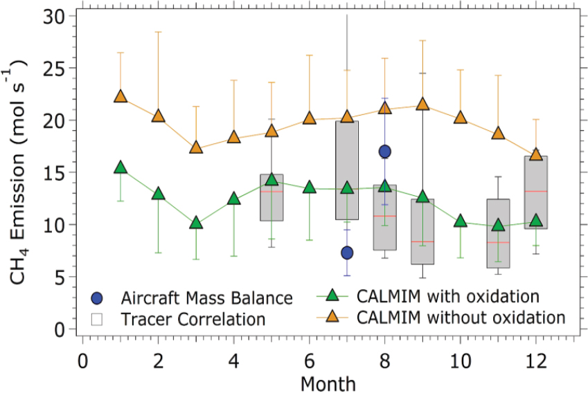
At specific sites, this model can provide a temporal framework for expected emissions with and without oxidation for comparison to field measurements. Figure 3.3 compares whole-landfill methane emissions for an Indiana landfill using an aircraft mass balance technique, tracer correlation, and modeled monthly emissions with and without oxidation (Cambaliza et al., 2017). Here the model provides a temporal framework for expected emissions using 30-year average weather data with and without oxidation for comparison to the field values. Importantly, cover-specific field measurements and modeling concluded that >90 percent of the total site emissions were derived from the daily working area, which constituted <10 percent of the total site area. This is directly attributable to an operational practice that is not universally practiced at U.S. landfills; namely, an underlying intermediate cover was stripped prior to vertical expansion for new cell development. Hence, new waste directly overlaid old methanogenic waste without an intervening cover, resulting in high emissions. At sites where this is standard practice, the total site emissions can be largely dependent on the daily filling area, and boundary conditions within the CALMIM model (e.g., methane at base of cover) can be readily adjusted to accommodate this practice. For many other sites, however, a high percentage of total site emissions can be attributed to intermediate cover areas, which typically cover large areas and have thinner cover soils than final covers (see Spokas et al., 2015, addressing California emissions). In general, estimation of landfill emissions using this model requires limited inputs: cover areas, their physical properties and thickness, and the extent of installed biogas recovery on a percent cover area basis.
CALMIM has also been applied in California to a new 2010 state-level inventory and compared with the existing 2010 state inventory using IPCC (2006) (which assumed 75 percent biogas collection efficiency and 10 percent oxidation; Spokas et al., 2015). The three most common California cover types used for this simulation were taken from an independent dataset developed by the California Department of Resources Recycling and Recovery (Walker et al., 2012). Site-specific emissions between the two inventories varied inconsistently in both directions due to the different drivers for emissions, namely, mass of waste using IPCC (2006) and, more realistically, the combination of soils and seasonal climate using CALMIM (see Figure 4.2).
Use of and further improvements to field-validated, process-based models (e.g., the California Landfill Methane Inventory Model) that rely on site-specific drivers for emissions (e.g., area, thickness, and texture of each cover soil; extent of installed biogas recovery; site climate) can provide more realistic estimates of methane emissions than current GHGI and GHGRP methods. In particular, robustly linking cover-specific oxidation to site-specific climate is warranted.
Coal Mines
Methane in coal can be generated thermogenically, as part of the coalification process,6 or biogenically owing to activity of microbes. Thermogenic methane is produced from coal organic matter by chemical degradation and thermal cracking mainly above a temperature of 100°C. In contrast, biogenic coal-bed methane is generated by the breakdown of coal organic matter by methanogenic consortia of microorganisms at lower temperature, usually below 56°C. Because of these two different mechanisms of generation, typically coals of low coalification levels are targets for biogenic methane, whereas coals of high coalification level may contain thermogenic methane (e.g., Mastalerz, 2014). Coal extracted by underground techniques is expected to have more methane because of its better preservation at greater depth. In addition, deeper coals typically have a higher coalification level because of deeper burial and also because their emissions are supplemented by the methane from affected underlying or overlying sediments. In contrast, shallow coal uncovered in surface mines has less methane primarily because of its easy migration through the shallow cover to the surface over geological time. However, methane content in coal can vary significantly between coal basins, between coal beds within the basins, or even within individual coal beds (e.g., Strąpoć et al., 2008), depending on coal rank, coal type, stability of associated clastic formation, and complexity of local geological and hydrological conditions, making methane emission predictions from coal mines difficult.
Emission Estimates
Active Underground Mines
In underground coal mining, activity data such as numbers of mines and quantities of coal produced are well known and emission estimates rely on stack-based sampling of
___________________
6 Transformation of plant biomass into peat and coal (Diessel, 1992).
underground mine ventilation systems and measurements of degasification volumes. These numbers are regularly reported to the EPA.
Ventilation systems in active underground mines are the largest source of coal-mining methane emissions. Gas emitted from walls and pillars enters the ventilation system of mines when it is not captured by boreholes. Methane emissions from ventilation systems are assessed based on the airflow and the methane concentration in the ventilation air. While ventilation flow measurements do not show large variations (being a function of the size and capacity of the specific ventilation fan), the methane content in the ventilation air can vary significantly in response to changes in coal-seam properties and to changes in daily coal production. The Mine Safety and Health Administration (MSHA) requires that trained MSHA inspectors perform mine safety inspections at least quarterly by testing methane emission rates at each coal mine. Air bottle samples are collected at the mine’s main ventilation fans along with airflow rate measurement. If emission levels are greater than 3.86 metric tons (or 200,000 cubic feet) per day, more frequent inspections take place, every 5-15 days depending on the emission level. MSHA maintains a database of measured methane emissions from all mines with detectable levels of methane in the ventilation air (MSHA, 2015). Independent of MSHA measurements, individual coal mines perform frequent methane emission measurements to ensure safe working conditions. Emissions are measured, typically weekly, with handheld methane detectors and flowmeters at the base of the ventilation air shaft in the mine. Continuous monitoring devices are used primarily to warn miners if methane concentrations exceed 1.0-1.5 percent, and these concentrations are not recorded. Consequently, gassy underground U.S. mines have high-resolution methane emission data collected underground.
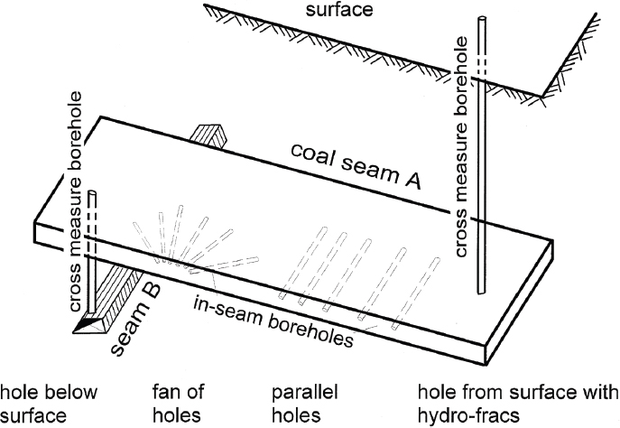
To prevent the occurrence of high methane levels in gassier mines, degasification of coal seams takes place prior to mining. This methane drainage reduces the gas content of the coal and decreases the risk of gas outbursts by decreasing the pressure in the rock formations (Karacan et al., 2011; Noack, 1998). Degasification is accomplished by in-mine horizontal boreholes or surface boreholes, and can be carried out before or after mining (Figure 3.4). In addition, post-mining wells recover methane from the overburden. While horizontal boreholes are often used to capture methane, surface boreholes are used to control seam gas and are typically vented into the atmosphere. The amount emitted is monitored daily or every few days at the wellhead with methane detectors and flowmeters. Some mines use continuous systems that monitor various parameters simultaneously.
In addition to emission assessment based on ventilation and degasification described above and used in the GHGI, various empirical models have been developed for
underground mines by various research groups in the United States and elsewhere (Kirchgessner et al., 1993; Lunarzewski, 1998). Empirical methods typically require only a few input parameters (e.g., coal production, gas content, and methane emission rate), but with the large number of parameters that influence emissions, the accuracy of the results is not always satisfactory (Karacan et al., 2011). To generate more accurate emission predictions from longwall mines, a modular software suite, Methane Control and Prediction,7 was developed using artificial neural networks in combination with statistical and mathematical techniques (Dougherty and Karacan, 2011). This software predicts emissions based on a number of parameters related to coal characteristics, mining conditions, and productivity, and can also conduct sensitivity analysis (Karacan et al., 2011).
Abandoned Underground Mines
Even though current methane emissions from abandoned underground mines account only for 9 percent of the total coal mine emissions, the increasing number of
___________________
7 See https://www.cdc.gov/niosh/mining/works/coversheet1805.html.
underground mine closings in recent years (e.g., decline from 523 in 2014 to 465 active mines in 2015 [EIA, 2016]) warrants efforts to improve emission estimates from this category. Gassy underground mines continue emitting methane after they are closed. The emissions are typically reduced compared to their active phase, but can still be substantial if gas can find conduits to migrate to the surface. The level of emissions varies depending upon many factors including gas content of the coal, mine flooding, the presence of conduits, the quality of mine seals, and the time since the mine closure. As discussed in Chapter 2, the EPA produced a methodology for abandoned underground mines in the United States (EPA, 2004), and annually reports methane emissions. In general, emission estimates from abandoned underground mines are based on the emissions during the active phase of the mine, assuming that emissions experience a hyperbolic decline after abandonment. The main challenge with the estimation of methane emissions from the abandoned underground mines is generation of an accurate decline curve. Methane adsorption isotherms, coal permeability, and pressure at mine abandonment are required to establish a reliable decline curve. Mine-specific data are used to fit the decline curve equations (Karacan et al., 2011).
Estimates from abandoned underground mines carry uncertainties related to a decline-curve generation. With an increasing number of underground mine closings, this is an important category that requires improvement in methane emission predictions.
Surface Mines
Surface coal mines release methane as overburden is removed and the coal is exposed. Methane can be emitted both from coal and associated clastic sediments (overlying or underlying rocks) that are affected by mining activities. Compared to underground mines, the level of emissions from the surface mines is much lower, primarily owing to low gas content of shallow coals that are mined from the surface. Therefore, emission measurements are not required for surface mines, and mine-specific emission data are rarely available. Consequently, the emissions are estimated using production data and coal and gas data. The GHGI uses Tier 2 country-specific emission factors and the volumes of the produced coal (EPA, 2005). As discussed in Chapter 2, the emission factor currently used in the United States is based on 150 percent of the in situ gas content of the coal (EPA, 2017b).
Efforts to develop direct methane measurements or mine-specific assessments in surface coal mines of the United States and elsewhere have also been attempted. For example, open-path Fourier-transform infrared spectroscopy followed by
Gaussian-based plume dispersion modeling showed that methane emission rates can range over an order of magnitude for a single mine (EPA, 2005). Use of a chamber method combined with measurement of surface gas emission flux in Australian surface mines yielded promising results but proved to be impractical to use. That technique required good measurement coverage to obtain a representative methane value for the mine, which, because of safety issues and lack of access to some areas, was practically impossible (Saghafi et al., 2004). Saghafi (2012) proposed a new Tier 3 method to estimate emissions from Australian surface mines based on an emission model that considered coal seams and surrounding horizons as individual gas reservoir units. The main input data required are in situ gas content, gas composition, and thickness of the gas-bearing horizons. The outputs of the model are gas emission factor, expressed in cubic meters of gas released per ton of coal extracted and/or gas emission density expressed in cubic meters of gas released per square meter of ground surface. In this method, two or three core drillings per mine are typically required to characterize a gas-emitting zone and to provide the main input of the model. Because of the limitations of the standard gas content measuring method, different limits of gas content measurability can lead to significant differences in the estimation of methane emissions.
These direct or mine-specific measurement efforts demonstrate that, although it is very desirable to estimate methane emissions for each surface mine, it is a highly challenging task because of variations in gas content and also because of the difficulty of gaining enough access to the sites to guarantee statistically sound measurement coverage.
Estimates of surface mine emissions are based on coal production data, often imprecise gas content, and assumed gas emission factors. Therefore, the estimates carry larger uncertainties than those from underground mines. However, underground mining has a much higher contribution to total methane emissions and therefore is a priority for efforts to improve methane emission estimates from coal mining.
TOP-DOWN TECHNIQUES FOR MEASURING METHANE EMISSIONS
Global Methane Monitoring Observations
Top-down emission estimates for methane, for the United States or any other region, rely on atmospheric measurements of methane and a quantitative understanding of the sources and sinks of methane in the atmosphere. Because U.S. emissions account
for a small portion of the global methane budget, and because the long atmospheric lifetime of methane allows emissions to be distributed globally, it is not possible to quantify U.S. emissions from atmospheric concentrations of methane without considering the contributions of global sources and sinks to methane concentrations. Global methane monitoring networks provide this information.
Monitoring of atmospheric methane was built on carbon dioxide monitoring efforts. It was initiated by the Rowland-Blake Group at the University of California (UC), Irvine, in 1978 and is ongoing, making these observations the longest-running time series of atmospheric methane concentrations. Air samples at approximately 45 sites distributed throughout the Pacific Basin from Alaska to New Zealand are collected four times per year, with many of the sampling sites located on remote islands in the Pacific and along the West Coast of the United States. Analysis of air samples also includes about 100 halocarbons and hydrocarbons, including some that are potentially useful for understanding sources of methane.
The National Oceanic and Atmospheric Administration (NOAA) Cooperative Air Sampling Network methane measurements started in 1983 and continue through today at more than 60 sites where volunteers collect samples that are shipped to the NOAA Earth System Research Laboratory (ESRL) in Boulder, Colorado, for analysis (Dlugokencky et al., 1994). The sampling frequency is about once per week, although at NOAA observatories, continuous observations are possible because air is sampled and analyzed in situ. Air samples have been collected from a variety of platforms including cargo ships, small aircraft, and tall telecommunications towers. NOAA aircraft and tower measurements are mainly at sites in the United States.
The Advanced Global Atmospheric Gases Experiment8 (AGAGE, sponsored by the National Aeronautics and Space Administration’s [NASA’s] Upper Atmosphere Research Program of Earth Science) started high-frequency methane monitoring observations in the mid-1980s at five globally distributed “baseline” sites (Cunnold et al., 2002) and continues today at over a dozen sites globally. The AGAGE network also measures more than 50 other atmospheric compounds, many of which are related to methane.
There is a wide range of signals to be detected in atmospheric methane using spatially distributed observations that are sustained over time. The latitudinal gradient of methane (the annual mean difference between the North and South Poles) is about 150 ppb, compared to the global average dry-air mole fraction (the ratio of moles of methane compared to number of moles of all components) concentration
___________________
8 See https://agage.mit.edu.
of ~1,850 ppb. Much smaller longitudinal gradients occur between the Pacific and Atlantic: 10-20 ppb, based on estimates of U.S. emissions and transit times across the United States. Differences in the Pacific-Atlantic gradient are particularly important for determining U.S. emissions because the Pacific is generally upwind and the Atlantic downwind of the United States. Near strong local sources, gradients can be much larger, hundreds to thousands of parts per billion over relatively small distances. The seasonal cycle of methane is on the order of tens of parts per billion, while decadal trends have ranged from <1 to >10 ppb yr–1.9 The ability to accurately quantify trends and spatial gradients that allow continental or regional emissions to be inferred places strong demands on the precision and accuracy of network observations.
Retrievals of column-average methane dry-air mole fraction (XCH4) from space-based remote sensing data such as the Scanning Imaging Absorption Spectrometer for Atmospheric Chartography (SCIAMACHY) and the Greenhouse Gases Observing Satellite (GOSAT) can provide useful information about the gradient across the United States, especially since these data could have much higher spatial and temporal resolution than is possible with in situ observations. However, precision and accuracy are worse than what can be achieved using the ground-based network, making the quantification of large-scale trends more difficult. Given the impact of stratospheric methane and topography on column-averaged methane abundances—which are measured by the satellite—full atmospheric inversions are required to infer total U.S. emissions. On the other hand, satellite retrievals are useful for detection of localized high emissions at small scales over which variations in topography, stratospheric methane, and tropopause height are not significant. Enhancements near strong localized sources can range from tens of parts per billion to greater than 500 ppb (Chen et al., 2016; Frankenberg et al., 2016; McKain et al., 2015; Thompson et al., 2016). For example, methane enhancements of 40 ppb were observed over the Four Corners region of the southwestern United States (Kort et al., 2014).
Uncertainties in top-down emission estimates are influenced both by uncertainties in atmospheric methane measurements and by uncertainties in the models used to estimate emissions based on atmospheric measurements (Box 3.1; for more detailed discussion of uncertainties, see Chapter 4). The uncertainty of network observations plays an important role in determining the sensitivity of the network to spatial and temporal variability of methane, and this translates into information about source distributions and their variability. The uncertainties of both the NOAA and AGAGE network observations are very small, amounting to only about 0.06 percent of global average methane mole fraction, meaning that the network observations are sensitive across
___________________
9 Ed Dlugokencky, NOAA/ESRL (www.esrl.noaa.gov/gmd/ccgg/trends_ch4/).
a large range of spatial and temporal variability. Using the current understanding of methane sources and sinks of methane, each 1-ppb increase of methane distributed globally requires emissions of 2.8 Tg methane (Fung et al., 1991). The 2016 uncertainty in mean modeled global tropospheric methane abundance (1.1 ppb) is equivalent to 3.1 Tg methane emissions globally, meaning that changes of 0.6 percent in the global methane budget can be detected (assuming a global total budget of 550 Tg methane
yr–1). On the other hand, space-based methane retrievals, which have a precision of 10-50 ppb, are difficult to use for accurately quantifying gradients between the Pacific and Atlantic and defining methane upwind and downwind of the United States. The high-precision methane observation networks currently in place provide a rigorous mechanism for tracking changes in global emissions.
International Methane Monitoring Efforts
In addition to methane network observations collected by NOAA, NASA (through AGAGE), and UC Irvine, monitoring of methane is conducted by many other nations and these measurements are important for understanding factors that influence the flux of atmospheric methane that enters the United States. For example, Environment and Climate Change Canada collects long-term observations at Alert, Nunavut, and other locations throughout Canada. A long-term record of methane for the well-mixed Southern Hemisphere has been collected at the Cape Grim Observatory in Tasmania by the Commonwealth Scientific and Industrial Research Organization, Australia.
The use of monitoring observations from multiple institutions can significantly improve data coverage; however, it is necessary to ensure that the data are of comparable quality and are calibrated to the same scale. To facilitate this, the World Meteorological Organization has set up a framework to ensure that data submitted to the World Data Centre for Greenhouse Gases (WDCGG) meet quality and calibration standards and that relevant metadata are distributed along with the data. The commitment to regularly submit data to the WDCGG varies, with some institutions providing frequent updates and others lagging by years. A map showing current sites for which greenhouse gas observations have been submitted is shown in Figure 3.5.
Monitoring observations have also been made from commercial aircraft by European, Japanese, and Australian investigators (Brenninkmeijer et al., 2007; Machida et al., 2008). These data provide information about the upper troposphere and lower stratosphere. Profiles are made during ascents and descents mostly in polluted urban environments, potentially making them useful for estimating urban emissions.
Monitoring of Related Atmospheric Trace Species
Global monitoring observations are also available for atmospheric trace species that are important for understanding the methane budget. For example, NOAA air samples are measured for 13CH4 by the Institute of Arctic and Alpine Research (INSTAAR) at the University of Colorado. This methane isotope is useful for attributing emissions to biogenic
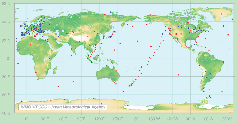
or thermogenic sources (Schaefer et al., 2016; Schwietzke et al., 2016). Methyl chloroform can be used to infer the strength of the chemical sink of atmospheric methane because its emissions are thought to be well known, and its only chemical loss, as for methane, is by reaction with hydroxyl radicals (e.g., Rigby et al., 2017). Measurements of methyl chloroform are made by NOAA/ESRL, UC Irvine, and the AGAGE network.
Observations of some hydrocarbons such as ethane and propane may also help to quantify emissions from petroleum and natural gas production since they are co-emitted with methane from this source. The ratio of the emissions of these higher hydrocarbons relative to methane varies considerably and is not well characterized at present (Allen et al., 2017; Peischl et al., 2015, 2016). However, both ethane and propane are increasing rapidly in the atmosphere, possibly due to increased petroleum and gas production in the United States (Franco et al., 2016; Helmig et al., 2016), although methane emissions from petroleum and gas production are thought to be stable (Bruhwiler et al., 2017; Schwietzke et al., 2016). Monitoring observations of some nonmethane hydrocarbons are currently being made in NOAA/ESRL air samples by both NOAA and INSTAAR, and by UC Irvine, and as in situ measurements at AGAGE stations.
Observations Using Remote Sensing Techniques
Observations of methane column abundance from satellite platforms may significantly increase the spatial and temporal coverage of observational constraints (Jacob et al., 2016) on forward and inverse models used to estimate emissions. Satellite measurements typically use methane absorption features in the shortwave or thermal infrared spectral range to derive methane abundances. Remote sensing in the shortwave infrared is based on absorption spectroscopy using the sun as a light source, which makes it very sensitive to methane in the entire atmospheric column, including near-surface variations (e.g., Buchwitz et al., 2000). However, using the sun as a light source excludes nighttime measurements. Retrievals in the thermal infrared use blackbody radiation from the surface and the atmosphere as the light source and are less sensitive to the surface, with peak sensitivity in the free troposphere (e.g., Wecht et al., 2012; Worden et al., 2013).
One of the primary advantages of remote sensing is that, in principle, it enables global, frequent coverage with a single instrument. However, satellite-based retrievals will never be able to be as accurate or precise as ground-based in situ instruments, as the measurements are always affected by other confounding factors such as aerosols, which can never be fully eliminated with passive remote sensing (see Chapter 4). If proven successful, future active remote sensing using Lidar (Light Detection and Ranging), such as the Methane Remote Sensing Lidar Mission Merlin (Pierangelo et al., 2016), might alleviate these caveats and enable year-round measurements from pole to pole. Active measurements are unlikely to achieve true global coverage, however.
Satellite observations of near-surface methane were spearheaded by the European and Japanese space communities. The first instrument to measure methane globally was SCIAMACHY, a near-infrared solar absorption spectrometer that has sensitivity to the near-surface atmosphere and a horizontal footprint size of 30 × 60 km (Frankenberg et al., 2005). Launched in 2002, data from SCIAMACHY were collected until 2012, when the instrument failed. Figure 3.6 shows an example of a long-term average of SCIAMACHY observations in the United States at 0.33° × 0.33° spatial resolution.
The Thermal and Near Infrared Sensor for Carbon Observation (TANSO-FTS, Hamazaki et al., 2005) is a similar, but higher spatial and spectral resolution (80 km2) instrument that was launched aboard GOSAT in 2009. The TROPOspheric Monitoring Instrument (TROPOMI)10 was launched in 2017 and has a much better spatial coverage at slightly better spatial resolution (7 × 7 km). The first U.S. satellite with high surface sensitivity will be the Geostationary Carbon Cycle (GeoCARB) Observatory (e.g., O’Brien et al.,
___________________
10 See http://www.tropomi.eu.
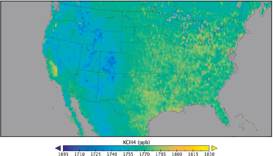
2016), promising higher spatiotemporal resolution. These higher-resolution instruments may allow for mass balance approaches to be used to estimate emissions with higher spatial resolution than is currently possible. Potential future missions might also be able to map localized plumes from space (Thompson et al., 2016; Thorpe et al., 2016), a technique that is currently only achieved using airborne platforms (e.g., Bradley et al., 2011; Buchwitz et al., 2000; Frankenberg et al., 2016; Hulley et al., 2016; Thorpe et al., 2014; Tratt et al., 2014). This strategy of very fine spatial resolution from space (<100 m) is followed by some commercial satellites such as GHGSat.11 Although the strategy is promising, it is unclear yet whether the commercial instruments are meeting the requirements and whether datasets will be publicly available.
___________________
11 See http://www.ghgsat.com/.
Continental-Scale Monitoring Observations
Atmospheric monitoring of greenhouse gases for the United States, including methane, occurs as part of the Global Greenhouse Gas Reference Network (GGRN) operated by NOAA and partners at universities and federally funded research institutions (Figure 3.7). The NOAA Cooperative Air Sampling Network is a subset of the NOAA GGRN. In addition to the GGRN, since 2012, Earth Networks, Inc., has established more than 40 monitoring locations throughout the United States. The company has closely collaborated with numerous government and academic organizations
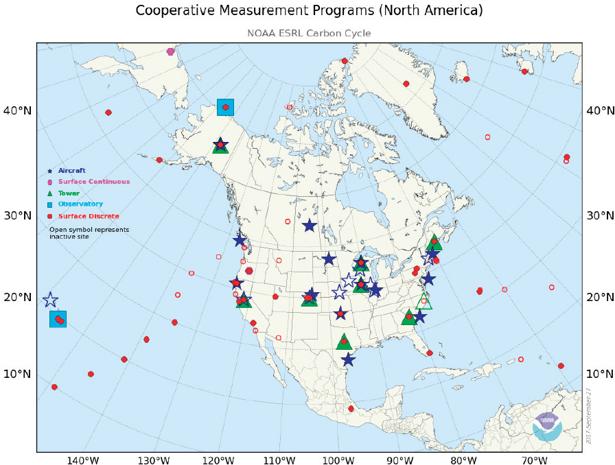
on urban measurement projects primarily in the Los Angeles Basin and Northeast Corridor. Data from the efforts are being made broadly available and several papers leveraging associated measurements have been or are in the process of being published (e.g., Brown, 2016).
Tall towers (~300 m) are a useful way to understand regional greenhouse gas (GHG) variability because as the wind changes direction, it is possible to detect signals from surrounding nearby sources. However, most of the NOAA tower network is not equipped to measure methane continuously, although there are some Earth Networks data available for urban areas, as noted above. Analysis systems deployed at tall-tower monitoring sites are based on commercial nondispersive infrared absorption sensors. Measurements of methane are not possible using these analyzers. However, cavity ring-down spectrometers (Crosson, 2008) or off-axis integrated cavity output spectrometers (O’Keefe et al., 1999), which do measure methane, have been installed at two tower sites in California. An example is Walnut Grove, California, where a cavity ring-down spectrometer was installed in September 2007.
Air samples have also been collected since the late 1990s using light aircraft (Sweeney et al., 2015). Currently, profiles of GHGs including methane are collected every 2 or 3 weeks at 17 locations (Figure 3.7) from the planetary boundary layer (0.5 km above sea level) to the free troposphere (up to 8 km above sea level). This aircraft program has provided information about large-scale horizontal and vertical methane gradients across the United States and their seasonal cycles. A climatology constructed from aircraft profiles clearly shows the accumulation of methane from west to east across the continental United States (Sweeney et al., 2015).
Regional Monitoring Observations
Regional atmospheric methane observations can be made using networks of tower sites similar to those used in continental networks, but at a smaller scale. For example, the California Air Resources Board (CARB) has a network of eight sites that have been continuously collecting methane data since 2010. The goal is to provide top-down (atmospheric) constraints on California methane emissions for comparison with bottom-up inventories (Figure 3.8; Hsu et al., 2010; Jeong et al., 2013, 2017). Regional tower and tall-building-based observations have also been made at the scale of individual cities, including Indianapolis (Lamb et al., 2016) and Boston (McKain et al., 2015).
Short-term, regional observations have also been conducted by aircraft, often in regions dominated by particular types of methane emission sources. Table 3.4 summarizes recent aircraft measurements that have been made primarily in petroleum
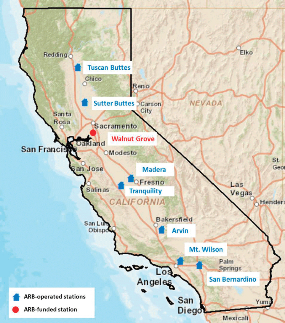
TABLE 3.4 Sample of Regional Methane Emission Studies Conducted Using Aircraft Plus Complementary Data
| Region Studied | Reference | Methods for Measurements |
|---|---|---|
| Fayetteville Shale | Schwietzke et al., 2017 | Aircraft-based measurements upwind and downwind of production region, complemented by ground-based data. |
| Bakken Shale | Gvakharia et al., 2017 | In situ samples near flares. |
| Bakken Shale | Kort et al., 2016 | Aircraft-based measurements of methane, ethane, carbon dioxide, carbon monoxide, and other compounds downwind of production region (but not upwind). |
| Bakken Shale | Peischl et al., 2016 | Airborne in situ measurements of methane, carbon dioxide, carbon monoxide, and ethane downwind of the production region (but not upwind); mass balance inversions. |
| San Juan Basin | Smith et al., 2017 | Airborne in situ samples for mass balance inversions. |
| San Juan Basin | Frankenberg et al., 2016 | Airborne imaging spectroscopy (remote sensing of methane plumes). |
| Barnett Shale | Karion et al., 2015; Smith et al., 2015 | Aircraft-based measurements upwind and downwind of production regions, complemented by extensive component and facility-scale emission studies. |
| Haynesville, Fayetteville, and NE Marcellus Shales | Peischl et al., 2015 | Aircraft-based measurements upwind and downwind of production regions. |
| Haynesville, Fayetteville, and NE Marcellus Shales | Peischl et al., 2015 | Aircraft-based measurements upwind and downwind of production regions. |
| Region Studied | Reference | Methods for Measurements |
|---|---|---|
| Marcellus Shale | Barkley et al., 2017 | Aircraft-based measurements of methane, carbon dioxide, and carbon monoxide, upwind and downwind of production region, complemented by facility-scale emission estimates; data used for aircraft mass balance inversions and atmospheric transport model optimization. |
| Indianapolis | Cambaliza et al., 2015 | Aircraft-based measurements with multiple transects upwind and progressively downwind of Indianapolis; methane and carbon dioxide measured using high-precision, high-time-resolution instruments, spectrometry at precise infrared wavelengths. |
| Denver-Julesburg | Petron et al., 2014 | Aircraft-based measurements upwind and downwind of production regions; methane measured using high-precision, high-time-resolution instruments, spectrometry at precise infrared wavelengths. |
| Southwestern Marcellus | Caulton et al., 2014b | Aircraft-based measurements downwind of production region (but not upwind); methane measured using high-precision, high-time-resolution instruments. Some measurements of single production sites. |
| Uintah Basin | Karion et al., 2013 | Aircraft-based measurements upwind and downwind of production regions; methane measured using high-precision, high-time-resolution instruments, spectrometry at precise infrared wavelengths; light alkanes analyzed from discrete air samples. |
| Los Angeles | Peischl et al., 2013 | Aircraft-based measurements of methane, carbon dioxide, carbon monoxide, and C2–C5 alkanes using high-precision, high-time-resolution instruments. |
| Los Angeles | Wennberg et al., 2012 | Aircraft-based measurements of methane, carbon monoxide, and ethane. |
SOURCE: Adapted and expanded from Allen, 2016.
and natural gas production regions. In general, these studies involve making measurements upwind and downwind of the source region during periods when the atmosphere is assumed to be well mixed. The instrumentation used in aircraft measurements can be varied, but generally relies on instruments with high time resolution and precision. Aircraft measurements are used to estimate regional emissions by multiplying (1) the methane concentration difference between upwind and downwind measurements by (2) the ventilation rate for the region. These types of observations have revealed significant regional variability in the intensity of methane emissions (units of methane emissions per unit methane produced) from petroleum and gas supply chain sources.
Estimating Emissions from Top-Down Observations
The observed spatial distribution and temporal variability of atmospheric methane is a “top-down” constraint on its sources and sinks. A variety of models are used to deduce information about emission and sink processes from spatially distributed time-series measurements of methane. At global, continental, and regional scales, forward and inverse modeling methods are used. At regional scales, some analyses employ mass balance approaches.
Both forward and inverse modeling approaches are powerful analysis tools that can increase understanding of the global and regional budget of methane. Inverse techniques are diagnostic because they allow a look backward in time to understand trends in emissions. They may provide guidance on whether policy aimed at mitigating methane emissions is effective, and they may alert scientists of increased emissions from Arctic wetlands and permafrost. Diagnostic modeling also can lead to improvements in prognostic modeling. By using inverse modeling to evaluate bottom-up models of emissions, improvements can be made to the bottom-up models, and the result may be better confidence in coupled climate–carbon cycle predictions.
Forward Methods for Estimating Emissions from Top-Down Observations
The forward approach involves use of bottom-up estimates of emissions and sinks, along with an atmospheric transport model to simulate atmospheric methane that can be compared with observations. Bottom-up estimates come from inventories of the type described in Chapter 2. Process model data or up-scaled flux observations can be used to prescribe emissions from natural wetlands, as well as methane uptake in dry soils (when soil acts as a sink). Differences between forward simula-
tions and observations provide information about possible gaps in understanding of unaccounted-for methane sources, which require adjustments to modeled source/sink processes to reach better agreement with observations.
The canonical example of this type of approach applied to atmospheric methane is the study by Fung et al. (1991), who comprehensively tested multiple possible methane budgets against observations such as the meridional gradient and seasonal variability of methane. They found a “best” global budget that totaled 500 Tg yr–1 in emissions, with losses due to uptake in soils and chemical sinks totaling 460 Tg yr–1. The imbalance between sources and sinks leads to increasing atmospheric methane, in agreement with the observed methane growth at that time. Fung et al. (1991) concluded that anthropogenic emissions were responsible for about 60 percent of the annual methane budget (recently supported by Saunois et al. [2016] using an ensemble of global inversions and bottom-up data). Interestingly, they also found that several budget scenarios could satisfy observational constraints, a finding that has important implications for the inverse approach.
Inverse Methods for Estimating Emissions from Top-Down Observations
While the forward approach uses models of atmospheric transport to convert emissions to atmospheric abundance, the inverse approach converts atmospheric abundance to emissions. Differences between atmospheric methane simulated using atmospheric transport models, first-guess emissions (i.e., “priors”), and observed atmospheric methane are used to solve for revised emissions. The numerical techniques employed range from simple mass balance approaches to data assimilation methods similar to those used in numerical weather forecasting. A very simple global inverse model approach using the global continuity equation for atmospheric methane was used by Dlugokencky et al. (2003) to propose that global methane was reaching a steady state during the late 1990s and early 2000s. Spatially resolved atmospheric transport models range from one-dimensional diffusion models (Bolin and Keeling, 1963), to zonal average models (e.g., Brown, 1993, 1995; Enting and Mansbridge, 1989; Tans et al., 1989), to detailed global atmospheric models with simple chemistry to calculate chemical loss (e.g., Bergamaschi et al., 2013; Bousquet et al., 2011; Bruhwiler et al., 2014).
Most inverse models are based on Bayesian inference, wherein new information coming from observations is systematically combined with bottom-up information (the priors) (Hein et al., 1997; Kandlikar, 1997). The resulting estimated emissions (posterior estimates) are in optimal agreement with both the priors and the observations, given
input uncertainties. In a Bayesian analysis procedure, the solution is strongly influenced by the relative weighting of information coming from the prior estimates and information coming from observations. This weighting is defined by estimated uncertainties of the prior emissions and observations. The observation uncertainty represents transport model uncertainty as well as measurement uncertainty; however, the latter is typically much smaller than transport model uncertainty for in situ observations. Defining the prior uncertainty estimates is challenging and may not be well constrained by independent information. For example, bottom-up estimates of emissions from inventories often lack associated uncertainty.
In addition, it is especially challenging to quantify model transport error, especially for measurement sites where the distribution of local sources may not be adequately known; therefore, it is difficult to determine whether model-data differences are due to a lack of knowledge of sources or transport errors. Díaz Isaac et al. (2014) found that, because of a lack of detailed knowledge of underlying source distributions, they were unable to definitively show that a high-spatial-resolution transport model was able to simulate observations better than a coarser-resolution global model.
For regional inverse modeling, McKain et al. (2015), among others, discussed the difficulty of disentangling transport errors from errors in specifying the locations of the emission sources. The atmospheric concentration data alone do not constrain both. Simulation methods for atmospheric transport are developmental, and current uncertainties limit the reliability of regional inversions.
Inverse models have proved to be an important tool, yet challenges to their usage remain, notably (1) the inability of the surface network to adequately reflect the full spatial variability of emissions, leading to multiple solutions that may significantly differ in spatial allocation of emissions and allocation of emissions among sources; and (2) the requirement that point measurements be accurately simulated with typically coarse-resolution transport models. Inverse modeling could provide information about variability and trends in atmospheric methane. It could also provide important insights into performance of bottom-up emission models, some of which may be coupled with climate models that are capable of predicting feedbacks between trace gas emissions and climate, leading to improved confidence in climate predictions. For example, by seeing how prior estimates of wetland methane emissions are changed by use of observations, biases in wetland emission process models may be identified and remedied.
Understanding global methane emissions is important for understanding U.S. emissions because knowledge of what is flowing into the United States is needed to
estimate what is being added to the atmosphere by the U.S sources. Houweling et al. (1999) found that compared to the a priori distributions of emissions, a posteriori emissions were reduced at high northern latitudes and increased at tropical and southern latitudes, a result obtained by many global inversions since (Bergamaschi et al., 2013; Bousquet et al., 2011; Bruhwiler et al., 2014; Houweling et al., 2014). Possible reasons for this include overestimated bottom-up emissions at high northern latitudes and underestimated bottom-up emissions at low and southern latitudes, as well as biases in model transport and chemical loss. In addition, it is difficult to rule out biases in atmospheric transport models. For example, a too-stable planetary boundary layer could systematically lead to underestimated emissions.
Adequate observational coverage in space and time is required to fully constrain inverse models at national or regional scales. There are only about 100 surface sites globally that measure atmospheric methane, and many of these sites are sampled only weekly, although a small number of sites collect continuous measurements. Many surface network sites have been selected to represent the background atmosphere remote from strong local sources. Some regions are therefore inadequately resolved by inverse models, for example, the tropics, where long-term monitoring is often logistically challenging and emissions are likely to be significant. Sparse data coverage has important implications for inversions; Hein and Heimann (1994) and Hein et al. (1997) used a full global atmospheric transport model to estimate global methane emissions and concluded that their estimated emissions reproduced large-scale features such as the interhemispheric methane gradient reasonably well, but not grid-scale emission variability.
Improving atmospheric transport models will also lead to more accurate estimates of emissions using inverse models. Patra et al. (2011) evaluated and compared a suite of atmospheric transport models for 1990-2007 using observations of methane, radon, SF6, and methyl chloroform at background sites and satellite retrievals of methane in the upper troposphere and stratosphere. Analysis indicated a considerable range in interhemispheric transport exchange time among models (1.2-1.8 yr), and differences due to vertical mixing, convection, and stratosphere-troposphere exchange were found. By using multiple inverse models, Locatelli et al. (2013) found that inverse modeling estimates of global methane emissions due to atmospheric transport differences could be as large at 27 Tg methane yr–1, comparable to an amount that could account for observed interannual variability. At continental scales, transport model differences led to even larger differences, with differences for North America of up to 36 Tg methane yr–1.
Coupling increased observations of atmospheric methane with improved measurements of important diagnostic quantities for atmospheric modeling (such as planetary boundary-layer depth) will likely help improve the accuracy of emission estimates, increasing observational constraints and providing critical datasets that may be used to improve atmospheric transport models.
Use of Satellite Retrievals in Inverse Models
Observations of column-average methane from satellite platforms may significantly increase the spatial and temporal coverage of observational constraints. Satellite data can be used in atmospheric inversions in the same way as ground-based observations. In fact, both data streams can be used in a single inversion, helping to ensure consistency and to point out potential biases in satellite data, which typically have lower accuracy due to their indirect measurement technique. Current satellite instruments have been shown to have persistent biases in space and time (e.g., Bergamaschi et al., 2013; Houweling et al., 2014) that must be accounted for if satellite data are to be assimilated into atmospheric inverse models. Remotely sensed observations of column methane using ground-based upward-looking Fourier spectrometry (e.g., the Total Carbon Column Observing Network) have been used to detect biases in the satellite data and to develop bias correction schemes (Houweling et al., 2014; Wunch et al., 2011). In terms of monitoring, successive instruments will be needed to monitor over multiple decades, and care will have to be taken to ensure that instruments are comparable.
Multiple studies have successfully used satellite data in atmospheric inversions (e.g., Bergamaschi et al., 2007; Cressot et al., 2014; Fraser et al., 2013; Fung et al., 1991; Houweling et al., 2014; Meirink et al., 2008; Turner et al., 2015) and underline the potential to reduce methane emission uncertainties on regional through global scales. Bergamaschi et al. (2009) noted good agreement between inversions using only surface network observations and inversions using surface observations and the revised retrievals at large scales. They also proposed that use of the satellite retrievals and estimation of emissions at grid scale resulted in information about how emissions vary at subcontinental scales, a result that was later questioned by Bousquet et al. (2011) based on comparisons of SCIAMACHY retrievals with model simulations of column-average methane using multiple inversion emission estimates. The use of their water-vapor-constrained bias correction led Houweling et al. (2014) to the conclusion that variability in tropical emissions is larger if SCIAMACHY retrievals are used in addition to surface observations and that the variability is more robust if bias correction parameters are not estimated along with emissions in the inversion.
Regional Estimates of Methane Emissions Using Top-Down Techniques
Some attempts to increase transport model resolution have been made using global models with increased horizontal resolution over regions of interest, a computationally cheaper alternative to global high resolution. Bergamaschi et al. (2005, 2010) applied a global model with two-way nested grids to estimate emissions from individual European countries using a nested grid of 1° × 1° resolution over Europe and a resolution of 6° × 4° over the global domain. Both studies found significantly higher emissions for parts of Europe compared to the values reported by the United Nations Framework Convention on Climate Change (UNFCCC). In particular, Bergamaschi et al. (2010) found emissions that were considerably higher than those of EDGARv4.0 (21 percent) and the UNFCCC (40 percent). Turner et al. (2015) used a global model with a nested high-resolution grid for North America and found much higher U.S. emissions than EDGAR and EPA estimates (40-43 versus 25-27 Tg yr–1), results consistent with other global time-dependent inversions (Bruhwiler et al., 2017; Saunois et al., 2016).
It is difficult to accurately simulate point measurements with a coarse-resolution model because of variability due to strong local sources, surface topography, and high-frequency atmospheric variability. For this reason, some recent studies have used regional models that simulate atmospheric transport at resolutions of 10 km or less. The most common strategy involves use of a Lagrangian particle dispersion model, such as the HYSPLIT (Hybrid Single Particle Integrated Trajectory Model; Draxler and Hess, 1997) or STILT (Stochastic Time-Inverted Lagrangian Transport; Lin et al., 2003) models, to simulate the backward trajectories of particles from measurement locations, keeping track of cumulative contact with the surface layer where emissions can influence the trace species concentrations in air parcels. A surface sensitivity or response function matrix is constructed, and inverse techniques are used to estimate sources, just as for the global case. Driving meteorology from high-resolution global analyses or regional models such as the WRF (Weather Research and Forecasting; Skamarock and Klemp, 2008) model is used to calculate particle trajectories.
The advantage of using a regional atmospheric model is that transport can be simulated at higher resolution and is likely to be more accurate than with a coarser global model. The disadvantage is that boundary conditions at the edge of the domain must be specified, and there is not good observational coverage to do this accurately. The solution is very dependent on the estimated boundary condition and Gourdji et al. (2012) found that use of different estimates of the boundary conditions could lead to differences in estimated fluxes of CO2 that were as large as the net annual flux over the region of interest, North America.
A Lagrangian approach with the Weather Research and Forecasting–Stochastic Time-Inverted Lagrangian Transport (WRF-STILT) model configuration was used by Kort et al. (2008) to analyze methane data collected by the CO2 Boundary Layer Regional Airborne–North America (COBRA-NA) airborne campaign. They concluded that the bottom-up emissions of EDGARv32FT2000 for North America were in good agreement with their top-down results. A later study using the same WRF-STILT model configuration concluded that for 2007 and 2008, anthropogenic emissions were significantly underestimated for North America (Miller et al., 2013). Emissions from ruminants and manure were found to be as much as a factor of 2 higher than estimated by the EPA and EDGARv4. In addition, Miller et al. (2013) found that emissions from fossil fuel production could be almost five times larger than estimated by EDGAR.
Bergamaschi et al. (2018) used both global inversions with high-resolution nested grids over Europe and Lagrangian inverse models to estimate European methane emissions. They found that the inverse estimates were substantially higher than those from bottom-up inventories and suggested that natural emissions from wetlands could be higher than bottom-up estimates. No systematic differences between global nested-grid and Lagrangian inversions were highlighted; however, the Lagrangian inversions used background methane from the global inversions, thereby eliminating a major source of difference between the two approaches. The study by Bergamaschi et al. (2018) also demonstrated the value of having a relatively dense network of quasi-continuous measurements; they were able to use a network of 18 sites, as well as additional sites with less-frequent discrete sampling.
Inverse modeling has also been used to estimate emissions at urban and petroleum and natural gas basin scales. For example, Lamb et al. (2016) used a WRF-STILT modeling system and measurements from the INFLUX campaign to estimate methane emissions for Indianapolis. They found significant differences between their inverse estimates and both bottom-up and mass balance estimates using measurements taken from aircraft. They found that 48 percent of methane emissions were from biogenic sources, with the remaining portion from fossil fuels, including citywide diffuse leakage. Jeong et al. (2017) employed a Bayesian inversion model to attribute methane and volatile organic compound emissions measured in the San Francisco Bay area. The authors conclude that landfills dominate the total emissions, and methane emissions from natural gas systems are approximately 0.3-0.5 percent of total natural gas consumed. Barkley et al. (2017) used the WRF regional model in Eulerian mode (i.e., without a Lagrangian calculation of sensitivity to surface sources) to estimate emissions from a portion of the Marcellus basin. They found agreement between their estimates and mass balance estimates based on aircraft observations, as well as leakage rates
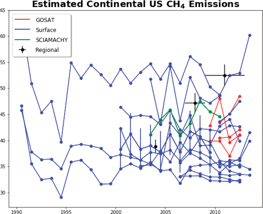
relative to total production for unconventional production and gathering facilities that were low compared to other basins (0.36 ± 0.09 percent).
Top-Down Estimates of U.S. Methane Emissions
Estimated emissions for the contiguous United States show a large spread, about 30-50 Tg methane yr–1 for 2000-2012 (Figure 3.9). These results are described by Saunois et al.
(2016) and represent an ensemble of global inverse model results contributed to the Global Carbon Project by the international global modeling community.12 The inversions use different combinations of observations (in situ and retrievals of column-average methane from SCIAMACHY and GOSAT), different atmospheric transport models, and different inversion setup choices (prior emissions and uncertainties, inverse technique). These differences account for the range in emission estimates. Inversions that sequentially estimate emissions over time (time-dependent inversions) are shown as lines, while inversions representing time averages are shown as points. Total methane emissions are shown because estimates of total emissions are more robust while source attribution is less certain due to sparse observations and inaccurate prior estimates.
Inversions using space-based retrievals of column average do not appear to significantly differ from those using only in situ observations, at least for the continental United States. The inversions by Wecht et al. (2014a) and Turner et al. (2015) give time-averaged estimates of U.S emissions, and both studies used a global modeling framework while solving for U.S emissions at high spatial resolution (100 km and 50 km). These studies were constrained only by column-average methane from SCIAMACHY and GOSAT. The inversion by Miller et al. (2013) is the only inversion that uses a regional modeling approach and their results lie well within the range of the other inversions.
Top-down estimates have also been produced for specific regions of the United States. The studies by Miller et al. (2013), Wecht et al. (2014a), and Katzenstein et al. (2003) found that emissions for the south central United States were higher than bottom-up estimates. Regional top-down estimates showed that emissions from fossil fuel production in the Four Corners region of the southwest are likely to be much higher than the EDGARv4.2 inventory (Kort et al., 2014; Turner et al., 2015). More recently, Smith et al. (2017) found that emissions in the Four Corners region have likely not changed since estimates were made for 2003-2009 using space-based column-average data, and that these estimates were consistent with the EPA 2012 inventory.
The top-down approach has also been used to estimate emissions from the state of California. Wecht et al. (2014b) used a global modeling framework and observations from the CalNex aircraft campaign and found that California methane emissions were about 30 percent higher than both the EDGAR and CARB (California Air Resources Board) inventories. Likewise, the study by Zhao et al. (2009) found that emissions in California were underestimated by 37 percent compared to prior estimates, the largest underestimate likely due to livestock.
___________________
12 See http://www.globalcarbonproject.org/methanebudget/index.htm.
Mass Balance Approaches for Estimating Emissions from Regional Aircraft Measurements
In contrast to forward and reverse inversion methods, the models used to estimate emissions for regional aircraft observations are much simpler. Aircraft transects are flown upwind and downwind of the study region. The total flux of air pollutants into and out of the region can be calculated by multiplying average concentrations of the air pollutant along the transect by wind speed perpendicular to the transect, the length of the transect, and the mixing height. Regional emissions are then estimated by subtracting the flux out of the region from the flux into the region.
There are several assumptions associated with this approach to estimating emissions. Since flights are typically done over multiple hours and upwind and downwind data collection can be done hours apart, the emission estimates assume that wind speeds, wind directions, and mixing heights remain constant over the sampling period. Since most aircraft flights sample at a single elevation or do only limited vertical spirals, the method also assumes that air pollutants (including methane emissions) are uniformly distributed throughout the mixed layer. These and other assumptions, such as limited sinks in the region, typically lead to uncertainty estimates for individual aircraft flights in the 20-40 percent range (see, e.g., Karion et al., 2015). Schwietzke et al. (2017) improved the mass balance methods by explicitly accounting for nonuniform upwind methane mole fractions in the planetary boundary layer in the study area. In addition, uncertainties were reduced by doubling the number of transects and employing a wind profiler.
Multiscale Observing Systems
For the reasons mentioned previously, accurate ground-based and spatially contiguous satellite observations should be seen as complementary to other approaches, with the combined systems overcoming weaknesses in the individual elements. The tradeoffs between frequent global coverage and lower accuracy and precision need to be taken into account when evaluating advantages and disadvantages of the accurate long-term ground-based network versus satellite data records. Accurate hemispheric averages and decadal variations can only be fully captured by long-term in situ sampling networks, which must be the backbone of any global observing strategy. On the other hand, space-based observation offers the unique capability to spatially map local gradients of atmospheric methane across the globe, revealing source processes and, potentially, emission rates.
With improving spatial resolution and temporal coverage, satellite data may also help identify key regions where the largest discrepancies between observed and expected (based on inventories) methane abundances exist. The Four Corners region in the United States is a primary example of how a regional hotspot was detected from space; the ensuing follow-up field investigations used both in situ samples and airborne remote sensing (e.g., Frankenberg et al., 2016; Kort et al., 2014; Smith et al., 2017). Using satellite data to identify key regions might lead to dedicated ground-based and/or airborne campaigns to quantify regional fluxes for individual source categories, ideally complemented with direct flux measurements on the ground. This can in turn improve inventory development on larger scales by identifying the drivers of underlying discrepancies per source category. This multiscale strategy could involve scales ranging from direct flux measurements at the facility level to the global view from space.
High-quality, long-term, multiscale surface and space-based data records are necessary for quantifying and tracking changes in methane emissions on regional scales.
COMPARISON OF BOTTOM-UP AND TOP-DOWN APPROACHES
Top-down and bottom-up approaches yield complementary information about methane emissions. Bottom-up methods provide information about the magnitudes and patterns of emissions from specific sources, and as a result they provide the type of information that is necessary to mitigate emissions. As shown in Chapter 2, however, bottom-up inventories of emissions may not account for all sources, and, as outlined in this chapter, the methods may have uncertain or inaccurate activity data and emission factors. Top-down estimates of emissions include emissions from all sources (even unknown ones) because they are based on atmospheric observations, but they may have difficulty in attributing emissions to specific sources and be subject to errors in atmospheric transport as discussed previously. Top-down approaches may also need to use prior emission estimates to constrain solutions due to sparse data coverage, and these may also have biases and errors that lead to biased top-down emission estimates. Both top-down and bottom-up measurements used to estimate emissions can also be spatially and temporally sparse, leading to biases. For example, when aircraft measurements are used to obtain data, the flights are typically limited to just a few days, and the measurements are generally done in midday when the atmosphere is well mixed. These measurements will therefore lead to information about emission sources that is limited to midday hours, and these emissions may be different than at other times of day, which limits direct comparisons with methane inventories such
TABLE 3.5 Comparison of Top-Down and Bottom-Up Approaches to Estimating Methane Emissions That Introduce Challenges in Estimating Emissions Using Both Approaches
| Approach | Top-Down Data | Bottom-Up Data and Inventories |
|---|---|---|
| Spatial scale | Facility to global | Individual site level to global |
| Temporal scale | Instantaneous to annual or multiyear averages | Generally reported as annual averages for inventory purposes from limited time duration data collected at various temporal scales |
| Source attribution | Involves use of models and assumptions as well as molecular and isotopic tracers | Calculated from source-specific activity data |
| Potential for missing sources | Measurements reflect all sources that contribute to observed atmospheric concentrations | May not account for all sources in a given region |
as the GHGI (Chapter 2). Table 3.5 summarizes issues related to missing or undocumented sources, source attribution, and spatial and temporal scales for top-down and bottom-up approaches.
The complementary information provided by top-down and bottom-up methods offers the opportunity to combine their strengths in coordinated measurement campaigns. Only a limited number of highly coordinated campaigns have been performed that utilize both types of methodological approaches, however, and the most comprehensive of these studies have been performed in regions dominated by petroleum and natural gas supply chain emissions.
In 2013, the Environmental Defense Fund organized a coordinated top-down and bottom-up measurement campaign in the Barnett Shale petroleum and gas production region in north central Texas. Multiple teams of investigators performed aircraft measurements of methane and ethane, leading to top-down emission measurements on multiple days. Several teams of investigators did ground surveys downwind of individual sites, collecting site-specific emission estimates for hundreds of petroleum and natural gas sites, including production sites as well as other, downstream sources. All of this bottom-up and top-down information was synthesized into a portrait of
methane emissions in the region (Zavala-Araiza et al., 2015) wherein estimates from both approaches converged, but this convergence was possible because of (1) a spatially resolved inventory wherein the national activity data for bottom-up estimates were supplemented by local counts of facilities and (2) enhanced sampling strategy and application of a statistical model to account for and characterize high-emitting facilities.
In the Fayetteville Shale natural gas production region in Arkansas, a top-down and bottom-up comparison was performed in 2015 with DOE and industry sponsorship (Bell et al., 2017; Schwietzke et al., 2017; Vaughn et al., 2017; Zimmerle et al., 2016, 2017). The study featured contemporaneous application of top-down and bottom-up techniques with site access and operational data from the major natural gas producers in the region to develop a spatiotemporally resolved bottom-up inventory. This effort found significant day-to-day variability in bottom-up emission estimates, depending on the nature of the planned natural gas production operations occurring on particular days. Because operations at individual sites varied from day to day, there was significant spatial variability in emissions from day to day. Top-down measurements confirmed the daily variability in emissions, and overall, the study confirmed that knowledge of both local facilities and daily operational schedules are important in comparing top-down and bottom-up emission estimates.
Coordinated, contemporaneous top-down and bottom-up measurement campaigns, conducted in a variety of source regions for anthropogenic methane emissions, are crucial for identifying knowledge gaps and prioritizing emission inventory improvements. Careful evaluation of such data for use in national methane inventories is necessary to ensure representativeness of annual average assessments.


