
Appendix G
Invited Paper: Use of Dispersion Modeling Tools in Optimizing Biological Detection Architectures
Disclaimer:
This white paper was prepared for the September 18-19, 2017, workshop on Strategies for Effective Biological Detection Systems hosted by the National Academies of Sciences, Engineering, and Medicine and does not necessarily represent the views of the National Academies, the Department of Homeland Security, or the U.S. government.
Prepared by David F. Brown
Argonne National Laboratory
1 BACKGROUND
In this paper we discuss the dispersion modeling tools and approaches employed to quantify the performance of biodetection architectures such as BioWatch. The overall analysis approach for determining functional requirements for potential biodetector networks was developed over a period of almost two decades and is designed to account for the inherent uncertainty in a future bioterrorism event. The threat of interest is defined as an aerosolized release of biological agent in an urban region and includes outdoor releases as well as releases in critical infrastructure facilities such as subways, airports, intermodal transit venues, convention centers, and arenas. Of course, the target, delivery system, and ambient conditions for a future attack are all unknown parameters. Therefore, the first step of the analysis is to survey these parameters in a Monte Carlo simulation or parametric sweep and generate the design-basis threat (DBT), that is, a library of credible attack scenarios against which the biodetector network is then optimized and/or the potential trade-offs of performance are assessed. By employing a statistical approach to scenario library construction, the detector performance results will be robust across the spectrum of both uncertainties and variations in DBT parameter space. We begin our discussion of the key modeling tools and then present their application to the design and optimization of biodetection networks and conclude with a summary of future directions.
2 KEY MODELING TOOLS
Physical modeling of aerosolized bioagent releases is the cornerstone of the overall biodetection architecture analysis and allows us to quantify impacts in significant detail. In this process, a single scenario is defined as a combination of the following parameters: (1) agent of interest, (2) release size, (3) target and release location at or within the target, (4) particle size, and (5) meteorological or facility or subway operating condition (including heating, ventilation, and air conditioning operations for buildings or subway operation characteristics). For each scenario, dispersion models that calculate bioagent (or chemical agent) spread within the various domains are executed. It is important to note that particle size is a critical parameter for any interior location as that governs the deposition rate, which depletes the plume and allows for assessment of surface sampling. The key modeling tools we use in BioWatch and other related studies are the Quick Urban and Industrial Complex (QUIC) model for outdoor releases (QUIC Home Page; Williams et al., 2002), the Below Ground Model for subway releases, and the CONTAM model for other indoor facilities (Dols and Polidoro, 2015). In the past several years the National Laboratory team has developed the ability to evaluate cross-domain dispersion so that the efficacy of an overall citywide network involving outdoor, subway, and facility detection assets can be assessed (e.g., subway to outdoor, outdoor facility, etc.). An example of a cross-domain model run for a notional subway system and outdoor area is shown in Figure G-1.
An additional consideration that we have recently evaluated in subway analyses is the effect of material that is deposited on patrons and then resuspended as they move throughout the system (Liljegren and Brown, 2015; Liljegren et al., 2016). This so-called fomite transport phenomenon can be very important in many instances and can lead to a significant increase in contamination. However, it also offers additional possibilities for detection in sensitive detection architectures. Additional considerations such as contact transfer (on people) and tracking by shoes are important as well, especially when considering postevent sampling considerations (Sippola et al., 2014).
3 ANALYSIS STRATEGY
The modeling tools described above are executed for thousands (or tens of thousands) of scenarios. This provides a scenario library to inform the design-basis threat discussed in Section 1. This library is the key part of the analysis as it is interrogated in a Monte Carlo analysis to assess both the biodetector performance and the detection architecture optimization. After constructing the scenario library, differing numbers of detectors with specified performance characteristics are modeled in the appropriate domain, and population exposure models are used to calculate the fraction of population “protected” (Fp). This metric has historically been the preferred performance evaluation metric for the BioWatch program and is defined in the next section. However, other metrics related to detection probability for certain casualty events have been used to assess overall performance, and these more easily convey results to the stakeholder community.
A further discussion of the merits and limitations of Fp and the other metrics examined in this analysis are covered in Section 4. Having evaluated the Fp performance of a given detector network layout, the detectors are then moved to new locations within the simulation domain until the Fp as evaluated across the entire scenario library is maximized. For BioWatch, this process is then repeated for differing numbers of detectors so that we can determine the additional benefit of each additional collector. The same overall methodology can be applied to different bioagent and chemical detectors in development to help refine performance specifications. An illustration of the overall analysis process for detector performance is provided in Figure G-2.
4 DEFINING PERFORMANCE METRICS
Before detailing the study parameters and the performance analysis results, it is important to note that all analyses related to detection system design must be conducted utilizing a design metric that is meaningful and relates as closely as possible to the desired mission of the detection architecture. For the BioWatch program, the goal of the program is to detect releases of biological agents in the air that have the potential to cause thousands to tens of thousands of casualties. By detecting these events that have the potential to cause catastrophic losses of life in a timely manner, the program serves to provide warning to the government and public health community of a potential bioterror event. We consider these a detect-to-treat paradigm, meaning that the early warning is meant to marshal required medical countermeasures before persons become symptomatic. Related studies for chemical detection are fundamentally different, as chemical detectors have a much faster response time (minutes), so they follow a detect-to-protect paradigm allowing for potentially affected persons to get out of harm’s way before they are adversely affected by the release.
Since the goal of the BioWatch program focuses on minimizing the impact of significant releases and supporting the response community in consequence assessment or management, the primary optimization metric for detector performance has historically been an impact-based fraction of population protected as defined in Equation (1) below:
Another useful statistic is the probability of detection for a given casualty count, given by
where we typically use Pd10k, Pd1k, and Pd1 (where N = 10,000, N = 1,000, and N = 1, respectively). We note that for facilities and subway work within BioWatch, Pd10k is generally not useful as it is often 100 percent once a few collectors are deployed and therefore that metric cannot assess the benefit of additional collectors.
Other common approaches to the design and optimization of detection system deployments involve designing the system to detect scenarios that involve a particular release mass of biological agent or focus on maximizing the probability of detecting all releases in a given scenario library. The use of these other metrics for system design may be appropriate for designing and evaluating individual detector performance, but they are generally not useful for optimizing op-
erational networks. For example, one may design a system to detect release sizes greater than a certain mass amount with 90 percent probability. This performance metric may be problematic, because the response community is not generally concerned with how much agent may be released. Rather, the key concern lies in how many people have been exposed or become casualties. It is for this reason that there is strong motivation to design detection systems with a metric related to impacts.
5 COMPARISON OF PERFORMANCE METRICS
Having provided a brief explanation of different metrics one might use to evaluate detector performance, it is worthwhile to further explain the advantages and disadvantages of each and how they relate and differ with one another. To illustrate the characteristics of different metrics, we will explore an example comparing the fraction of population protected and probability of detection performance for a notional (unoptimized) network for an outdoor venue. These are illustrated in Figure G-3.
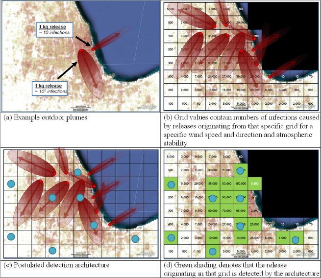
To compare Fp and Pd metrics, Figure G-3(a) shows a representative outdoor computational domain with two plumes featuring the same release size, but differing metrological conditions. As can be observed, the release that remains over land results in approximately 10,000 infections, while the other release location infects approximately 10 people, as agent is quickly carried over water. This example shows that it is the combination of the release size, location, spatial population distribution, and meteorological condition that determines impact. Similarly, in considering facilities and subways, the same general considerations apply as releases can quickly exit the facility or subway, causing minimal impact (but substantially more serious ones in other domains). For the purposes of calculations, the computational domain area of interest is divided into cells where releases can occur and detectors deployed as demonstrated in Figure G-3(b) (not all of the plumes in the grid are visualized in the figure). The number of infections caused by releases originating from each grid for each given meteorological condition are then calculated and compiled into a single scenario library. Detector architectures are then postulated and optimized using standard techniques, and releases that originate in each grid are evaluated based on whether they are detected by the architecture. In Figure G-3(d), green shading denotes that the release originating in that specific grid was detected by the postulated detection architecture. The nonshaded grid locations denote that a release originating from that location was not detected by the postulated architecture.
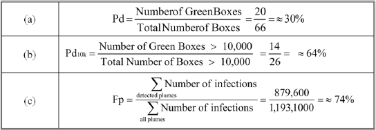
Having determined the impacts for all the scenarios and which ones are detected and not detected by the detector architecture, one can evaluate the performance using a variety of metrics. Below in Figure G4 are the resulting design metric performances as calculated by the fraction of population protected (Fp), probability of detection (Pd), and probability of detection for scenarios that cause greater than 10,000 infections (Pd10k).
When comparing the performance of the various metrics, one can observe that the notional network appears to have poor overall performance when measured by Pd; however, the architecture does a reasonable job of detecting attacks that cause large infections, measured by Fp and Pd10k. It is for this reason that the application/mission space of the detection systems are taken into account to evaluate the true value of the system.
In an effort to further compare and contrast various design metrics, some commonly used detector performance metrics are listed, along with some advantages and disadvantages of each, in Table 1. An additional example of how these metrics are used to assess overall performance is demonstrated in Figure G-5. Shown here are notional examples of how we can assess the performance of detection networks based on bioagent detector sensitivity and the number of detectors deployed in a particular venue. In particular, Figure G-5(a) shows a common characteristic that is the basis for determining the number of detectors necessary in a system of a known sensitivity (such as BioWatch) and how we can determine the proper allocation of assets assessing the marginal benefit of each additional detector.
TABLE G-1 Comparing Options for BioWatch Performance Design Metrics
| Fraction of Population Protected (Fp) | Probability of Detection (Pd) | Fp with Release Size Thresholds | Pd with Impact Thresholds | |
|---|---|---|---|---|
| Advantage |
|
|
|
|
| Disadvantages |
|
|
|
|
6 SUMMARY
The modeling tools and detection performance metrics discussed in this paper have been developed over the past two decades and are in a state of continual improvement through integrating results of experimental studies, both in the laboratory and in complex urban environments (Brown et al., 2009, 2013, 2015). This includes cross-domain dispersion experiments such as the 2016 Underground Transport Restoration experiments in New York City (DHS, 2016). Our experience has shown that every jurisdiction and stakeholder community, as well as our federal partners, has different needs and diverse questions as to detection performance and response strategy development. As new detection technologies become available, application of the ideas discussed here will be continually evaluated, as we advance both the scientific phenomenology of the underlying physical models and the optimization tools employed to assimilate their results.
7 REFERENCES
Brown, D., J. Liljegren, M. Sippola, M. Lunden, and D. Black. 2009. The 2007/2008 Washington, D.C. Subway Tracer Transport and Dispersion Experiments: Measurements and Analysis. Argonne National Laboratory, FOUO Technical Report ANL/DIS-09-03.
Brown, D., J. Liljegren, D. Black, and M. Lunden. 2015. The 2009/2010/2012 Boston Subway Tracer Transport and Dispersion Experiments: Measurements and Analysis. Argonne National Laboratory, FOUO Technical Report ANL/GSS-15/3.
Brown, M., A. Gowardhan, M. Nelson, M. Williams, and E. Pardyjak. 2013. QUIC transport and dispersion modelling of two releases from the Joint Urban 2003 field experiment. International Journal of Environmental Pollution 52:263–287.
DHS NYC (Department of Homeless Services New York City) Subway Tracer Studies, May 9-13, 2016. https://www.dhs.gov/sites/default/files/publications/DHSNYCSubwayTracerStudiesMay9-13%2C2016.pdf (accessed February 21, 2018).
Dols, W., and B. Polidoro. 2015. CONTAM Users Guide and Program Documentation, Version 3.2. NIST Technical Note 1887. doi: 10.6028/NIST.TN.1887.
Liljegren, J., and D. Brown. 2015. The Argonne Below Ground Model: Passenger Dynamics, Exposure, and Fomite Transport. Paper presented at the 83rd Military Operations Research Symposium, June 22, Washington, DC.
Liljegren, J., D. Brown, M. Lunden, and D. Silcott. 2016. Particle deposition onto people in a transit venue. Health Security 14(4):237–249.
QUIC (Quick Urban & Industrial Complex). Home Page. http://www.lanl.gov/projects/ quic (accessed February 21, 2018).
Sippola, M., R. Sextro, and T. Thatcher. 2014. Measurements and modeling of deposited particle transport by foot traffic indoors. Environmental Science & Technology 48:3800–3807.
Williams, M., M. Brown, and E. Pardyjak. 2002. Development of a dispersion model for flow around buildings. 4th AMS Urban Environment Symposium, Norfolk, VA, Paper J1.12.


