
7
Analysis Techniques for Small Population Research
The final technical session of the workshop covered analysis techniques for small population and small sample research. Rick H. Hoyle (Duke University) described design and analysis considerations in research with small populations. Thomas A. Louis (Johns Hopkins Bloomberg School of Public Health) described Bayesian methods for small population analysis. Katherine R. McLaughlin (Oregon State University) spoke about estimating the size of hidden populations. The session was moderated by steering committee member Lance Waller (Emory University).
DESIGN AND ANALYSIS CONSIDERATIONS IN RESEARCH WITH SMALL POPULATIONS
Rick Hoyle covered how to maximize the acquisition of data, design and measurement, and analyses that can be done with small sample data given the constraints. He broke his presentation into the following parts: informative analysis, a definition of small in a data context, an explanation of the finite population correction factor, and design and measurement qualities that optimize research when samples are small. He concluded with a discussion of multivariate possibilities that might be applicable in small sample situations.
Informative Analysis
Data analysis is informative when it addresses the question that motivated the research. Sometimes, however, the researcher may need to reframe
the question in a more modest fashion given the constraints of the data. Importantly, the researcher needs to understand the assumptions of the data analytic method and ensure that the data correspond with and meet those assumptions. To the extent that hypothesis testing is needed, it is important to have some notion that the study is sufficiently powered to detect meaningful effects. As a compromise, the researcher may be able to conduct descriptive analyses that can set the stage for future research.
What Is Small?
Hoyle listed several attributes desired of a study, saying that if the sample size makes any of these problematic, then the sample is “small.” First, researchers want a situation in which the outcome of the data analysis is not highly influenced by one or two cases. Second, researchers want valid estimates of parameters and standard errors. Third, it is important that parameters estimated using iterative methods result in convergence to valid estimates. Finally, the relationship between the final sample size and the “size” of the effect to be determined should be appropriate.
Hoyle noted “small” cannot be an excuse in every case. Sometimes a sample is small because of constraints such as a small population or insufficient resources. There are certainly conditions under which a researcher has small samples but could have done better, perhaps with more resources or more time and effort in recruitment and retention. Because small sample data analyses require compromises, it is difficult to justify those situations when it would be possible to do better.
Finite Population Correction
In a small sample situation, he said, and in particular when sample size is constrained by population size, one potential approach for increasing the power of statistical tests is to use the finite population correction. To introduce this concept, Hoyle first introduced the sampling fraction, f = n/N, where n is the sample size and N is the population size. If f = 1, then there is a census. In that case there is no sampling error, though there could be error from other sources. When the value of f is not 1 but approaches 1, the proportion of the population from which there are data has increased, and the sampling error in estimating the population parameter is less than it would be with fewer observations.
Conversely, f approaching zero reflects the usual situation where the size of the sample is small relative to the size of the population. When f is greater than .05, then the power of statistical tests can be improved through use of the finite population correction factor,
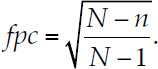
Hoyle provided an example with a population size of 200 and a known standard error of 10. He explored the situation in which the sample size varied from 10 to 175, noting that the standard error associated with each sample is equal to 10 times the finite population correction. In this case, the finite population corrected standard error ranged from 9.77 to 3.54. The standard error of 9.77, associated with n =10, is very close to the population standard error. This is the situation where f = .05. With larger samples, above that point the sample standard deviation starts to be reduced. With a sample of size 175, almost 90 percent of the population is included in the sample, so the sample standard error (representing the uncertainty in the unknown remainder of the population) is substantially smaller than the value of 9.77.
If researchers know they will be operating in a small population context and inferences are desired only on that population, this relationship can be used to estimate the sample size needed to achieve a certain level of power. Researchers can use standard power tables to determine the appropriate sample size for an infinite population. Second, the sample size adjusted for a finite population can be computed,
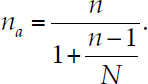
Hoyle observed, for example, that if the usual required sample size is 150 for a very large population, but the population size is 200, the adjusted sample size is 86 to achieve the same level of power. On the other hand, if the usual required sample size is 50, but there is a population size of 200, the adjusted sample size is 41.
Hoyle acknowledged inferential limitations associated with this approach that may or may not matter depending on the goals of the research. He noted that the finite population correction assumes random sampling without replacement and accounts for a reduction in sampling error as f increases toward 1. It allows inference about the state of this population (200 in his example above) at the point in time of the sampling. It does not support inference about another population that may be like this one, nor does it represent this population at any other point in time.
Design and Measurement Qualities That Optimize Research
Hoyle suggested several ways to strategically think about adjustments in the study plan that would help to support inference in a small sample situation. He showed a general t-test—the ratio of a parameter estimate to its standard error. If the goal is to detect a significant effect, there are two options for increasing t: increase the parameter estimate or decrease the standard error.
He gave examples of approaches for increasing the parameter estimate. For people in the treatment group, one approach is to sharpen the focus and increase the dosage of the treatment, whatever it might be. The choice of the control condition is also critical. There should be no hint of the active component of the treatment present in the control condition. The treatment should be directly focused on the causal mechanism.
Hoyle stated that measurement is another important aspect of a small sample study. The outcome measure chosen should be reliable to minimize attenuation due to unreliability and sensitive to maximize the odds of detecting difference or change. Hoyle suggested that researchers frequently do not consider all factors that may be affected by the treatment and the causal mechanism at play to understand where the treatment may create variability that can help or hinder in measuring the outcome.
Given the limitations on statistical power for a given treatment, it might be difficult to demonstrate an effect on the desired long-term outcome. However, there may be more proximal outcomes that relate to behavior change. He suggested that it may be known that these behaviors ultimately translate into differences in the outcome of greatest interest. However, the study may be better powered to detect an effect if the researcher focuses on those proximal outcomes.
Hoyle moved on to discuss the other way to increase the value of a t-statistic: decreasing the standard error of the parameter estimate. The standard error depends on the sample size, decreasing if the sample size is larger. Research is constrained by the number of people who participate in the study; thus, recruitment and retention are critical. Moreover, among the people who participate, some individuals may not provide complete information. Hoyle urged use of all data in an analysis, even if the data from some sampled people are incomplete. He noted that analytic models that allow the researcher to include all the data available in every analysis are preferred, and there are many accessible methods of dealing with missing data that create the possibility for leveraging the data that have been provided. Examples include multiple imputation and model-based methods such as full information maximum likelihood in structural equation modeling. These support the incorporation of a missing data mechanism in the model and allow inclusion of auxiliary variables.
In trying to increase the test statistic, Hoyle discussed the statistical analysis itself, using as an example a general linear model equation with outcome variable y, and the treatment variable x1. One can consider two different models: a simple one, with only x1 and y, and another multiple regression that includes x1 and y as well as other auxiliary variables that help to explain the variation in y. Including these covariates in the model, assuming that they really do account for some of the variation in y, reduces the standard error of the estimate of the coefficient on x1, increasing the power of the test. While these covariates may cost in terms of degrees of freedom, they may substantially reduce the error term in the equation, the denominator of the test statistic. This increases the likelihood of detecting an effect without really changing the estimate itself.
Multivariate Models
Hoyle noted recent research on pushing the assumptions related to sample size with regard to multivariate techniques. He said people want to use these techniques because many research questions being posed are, by their nature, multivariate questions and may require multivariate analyses.
Hoyle said that a scan of the literature1 reveals substantial evidence of people using so-called large sample multivariate techniques with samples that are clearly small. He reminded the audience that a multilevel model in which the second level, the cluster level, has fewer than 30 clusters is considered small. Growth models, exploratory factor analysis studies, and structural equation models with fewer than 100 participants are also considered small. Evidence of use of these techniques despite small samples, he said, leads him to conclude that people are posing questions that require these analyses and are highly motivated to use them to address those questions. He noted that research questions appropriate for multivariate analysis with small samples are likely to require data that are clustered, concern unobserved influences, and focus on patterns of change over repeated assessments.
Hoyle noted that multilevel modeling assumes continuous measures, four to eight predictor variables, no missing data, two or fewer cluster-level random effects, at least five observations per cluster, and an inter-cluster correlation of about 0.2. For multilevel modeling, small might be considered fewer than 40 clusters. With fewer than 20, it is clear that the standard application of the model should not be used. However, he noted that there are ways to handle situations in which the number of clusters creeps down to a low point. Approaches range from restricted maximum likelihood, to
___________________
1 See the bibliography prepared for this workshop: http://sites.nationalacademies.org/dbasse/cnstat/dbasse_181256 [March 2018].
restricted maximum likelihood with the Kenward-Roger correction, to wild cluster bootstrap.2
Hoyle noted that there is good news in multilevel modeling with an ecological momentary assessment (EMA) study that involves repeated sampling of a subject’s current behaviors and experiences in real time. In this situation, having 40 people is reassuring. Forty people with five observations of each person puts the researcher in a territory where multilevel modeling can be used responsibly.
Hoyle noted an interesting, just-published application.3 It uses the finite population correction factor in a multilevel model when the level two variable represents a small cluster population. Interestingly the authors argue that the usual choice by people using multilevel modeling is a fixed effect model versus a random effects model. If a fixed effect model is assumed, then the desired inferences deal only with the instances of the clusters in the data. Ordinarily, he said, that is not what is needed; if so, the finite population correction can be used to increase the power of the test. If a random effect model is assumed, the result is essentially an infinite population assumption.
Hoyle concluded by noting that structural equation modeling with fewer than 200 people is considered small sample territory, even for simple models with moderate loadings (0.5 to 0.7) and for moderately complex models of three or four latent variables. With fewer than 100 observations, the standard assumptions do not apply and structural equation modeling should not be used. He noted that typical assumptions are continuous measures and a near-normal multivariate distribution. Researchers should consider the magnitude of loadings on latent variables, the number of latent variables, and the number of indicators per latent variable. He suggested that researchers consider using sample size–corrected versions of the chi-square estimate, such as Bartlett, Yuan, or Swain corrections. He noted that the Yuan correction performs well with 25 or 50 sample observations. The final alternative noted is to limit model complexity.
Person-level dynamic modeling applies to the situation when there are enough data from a single person to draw inferences about the impact of an intervention or naturally occurring change with regard to that person (case). This technique is useful if there are a relatively small number of people in a study with a particularly long body of measurements for each person made in a common time frame. With this situation, the new sample
___________________
2 McNeish, D. (2017). Challenging conventional wisdom for multivariate statistical models with small samples. Review of Educational Research, 87:1117-1151. doi: 10.3102/0034654317727727.
3 Lai, M.H.C., Kwok, O.M., Hsiao, Y.Y., and Cao, Q. (2018). Finite population correction for two-level hierarchical linear models. Psychological Methods, 23:94-112. doi: 10.1037/met0000137.
size is the number of common observations made on each person. The analysis may be a person-level factor analysis of latent structure. Even though measurements are made over time, time is not considered in the analysis.
Hoyle provided an example of a small study of a heterosexual4 couple who on the day they married were recruited into a study. For 6 months, they each provided positive and negative affect data every day. Researchers ultimately ended up with 182 observations of two people across time. These data were used to examine the effect of one spouse at a point in time on the other spouse’s affect later. This study showed the woman’s affective experience was more likely to be influenced by the man’s than the other way around.
Hoyle pointed to person-level dynamic modeling in a meta-analysis of social skills interventions on autism spectrum disorder children.5 These models incorporate time to allow modeling of intra-individual change over time and use lagged covariance matrices that permit modeling of within-lag covariances between variables, autoregressive covariances (for stability), and cross-lagged covariances (for prospective relationships between variables). Additionally, he said, person-level data can be chained or analysis done using multigroup structural equation modeling. The study found that person-level dynamic modeling can allow for models that match the complexity of research hypotheses and allow researchers to do sophisticated multivariate causal mechanism analyses, despite a small number of participants.
BAYESIAN METHODS FOR SMALL POPULATION ANALYSIS
Tom Louis described Bayesian methods and their potential for use in small population analysis. He noted that for small populations, or at least small samples, inferences can seldom stand on their own. It is not just the sample size, but the sample size coupled with inherent variation. He noted that even with a very large population with a very small event rate, there is a potential for an unstable situation. A researcher cannot necessarily rely on large sample assumptions to make inferences. He suggested that a strategic approach would be to look for some kind of modeling combined with stabilization. He noted that many different approaches can get away from each molar unit standing on its own, such as aggregation. He referred to earlier presentations that touched on the effects of spatial aggregation (see
___________________
4 Ferrer, E., and Nesselroade, J.R. (2003). Modeling affective processes in dyadic relations via dynamic factor analysis. Emotion, 3:344-360. doi: 10.1037/1528-3542.3.4.344.
5 Nelson, T.D., Aylward, B.S., and Rausch, J.R. (2011). Dynamic p-technique for modeling patterns of data: Applications to pediatric psychology research. Journal of Pediatric Psychology, 36:959-968. doi: 10.1093/jpepsy/jsr023.
Chapter 3), remarking the same situation holds for sociologic aggregation. His preference, he said, is to keep things at the molar level and let a model do the work, being careful to ask the right question.
Bayesian Models
Louis said that, as discussed by Hoyle, regression functions and equations are attractive. However, he said that he would focus on Bayesian empirical-based hierarchal models that borrow information across units. Bayesian formalism, the engine of Bayesian analysis, forces thinking that produces effective approaches. He gave an example of trading off bias and variance for a linear model. He assumed a situation with K individuals or units: small areas, social domains, or institutions with an underlying feature of interest. Situations might include poverty in a small area, such as a school district, or a treatment effect. He then assumed a direct survey estimate that is unbiased and has a variance estimate. It may be that the variance estimate may be so high for some units as to not support desired comparisons. In addition, there may be unit-specific attributes, some covariates, such as tax data, that can be used to build a good regression equation. Nothing in the Bayesian approach eliminates the hard work needed to develop a good model, he stressed. The regression model can be used to produce estimates that may be quite stable; however, the unit-level estimates are likely to be biased. Now there are two estimates, the direct estimate that is unbiased but has high variance, and the regression estimate that may be biased but has lower variance. In this context, Bayesian modeling suggests a middle ground—an estimate that is partway between the direct estimate and the regression estimate. The Bayes estimate is a third estimate, a weighted average of the direct estimate and the regression estimate. The weight applied to the direct estimate will be close to 1 if the direct estimate has low variance relative to the regression estimate. However, if the direct estimate has high variance relative to the regression estimate, the weight on the regression estimate will be higher.
Examples of Bayesian Approaches
Louis’s first example was estimating the prevalence of modern contraceptive practices in Uganda and other African countries using a sample survey, where each woman reported about her contraceptive device uses (yes or no) along with her own covariates such as age and household income. Prevalence was estimated using a logistic regression with covariates and a random effect for enumeration area that allowed learning from other areas and previous survey waves. He demonstrated that the Bayesian approach, also called a shrinkage approach, resulted in estimates with reduced vari-
ance relative to the direct estimates, and noted that with careful modeling, reduced mean squared error.
He pointed to another example concerning bone density loss in women.6 It was written so that positive values are bone loss. The positive trend related to the age of the woman suggests a nonlinear bone density loss and perhaps that a quadratic loss might be reasonable. This example used an empirical Bayes approach to calm the variation in the estimates. The idea is each woman provided a few measurements on her bone density loss. Hui and Berger fit a locally linear model to each woman and combined those estimates accounting for the fact that the women were of different ages. The direct estimates were highly variable. Combining these estimates with the model results calmed the variation. Louis noted that other applications using more data have indicated that the combined results are more accurate. He concluded that many applications have shown that this kind of an approach is very effective if carefully done.
A real-life use of the empirical Bayes approach relates to insurance merit rating, where next year’s premium is based both on a person’s experience and on how that person relates to others in her or his risk group. The approach has proven very effective for insurance companies and insureds.
Louis also noted that another, perhaps underappreciated and underused, aspect of empirical Bayesian approaches is to stabilize variance estimates themselves. He noted that this is less controversial than stabilizing the direct estimates but is used relatively infrequently. The approach is similar to what he described earlier, but the distributions involved are not Gaussian.
Louis provided an example related to cancer. In the mid-1980s, researchers summarized the result of carcinogen bioassays by preparing two-by-two tables summarizing 50 rodents per group. Group C had no rodents with tumors, while Group E had 3 rodents with tumors. The pathologists said the tumors were biologically significant, while the statisticians said the tumors were not statistically significant.
Louis’s first point was that researchers from different disciplines need to communicate better. He argued a better approach might be to build history into the statistics, especially if there is historical information for the same species/strain of rodent in the same lab in a recent time period. For example, if there had been previous work with 450 rodents, none of which showed the tumor under condition C, then pooling data from the two studies provides a more convincing argument. In this situation, the three tumors under condition E are both statistically and biologically significant. He
___________________
6 Hui, S.L., and Berger, J.O. (1983). Empirical Bayes estimation of rates in longitudinal studies. Journal of the American Statistical Association, 78:753-759.
commented that though pooling the two data sources helps in this example, in general a more formal Bayesian model should be built.7
Louis pointed to recent work8 on combining evidence across data sources. This study showed how to take a focused, well-done, not necessarily highly precise study and stabilize it with a much larger study that does not have all the detail. This involves matching some marginal estimates and letting stabilization take place. There were some constraints making sure study estimates were consistent with the externally determined controls. In the survey world, this is benchmarking and more generally to matching margins in contingency tables. For an epidemiologic application, it could be considered using external prevalence data as part of a case control study to support calculation of odds ratios and risks. The key question in these applications is whether the stochastic features of the internal and external data are sufficiently similar. This type of decision requires some judgment and discussion. Louis observed that this work resonates with discussions about external validity and representativeness, noting several papers on the issue are included in the workshop bibliography.9
The survey world is dealing with Bayesian approaches. For example, Bell and Franco (2016)10 used the American Community Survey to stabilize estimates of disability from the Survey of Income and Program Participation. The formulas exploit the correlation between those surveys, which in this case was about 0.82. Using basic procedures, the authors achieved about a 19 percent reduction in the mean square error. Incorporating bivariate models produced about a 43 percent reduction in mean square error.
In the mid-1990s, CNSTAT convened a panel study, called the Small Area Income and Poverty Estimates (SAIPE) program, funded by the Department of Education to review and assess an effort to improve small area estimates of income and poverty.11 The program produces estimates of the percentage of school-age children in poverty in most school districts in
___________________
7 For an example of how to do this, see Tarone, R. (1982). The use of historical control information in testing for a trend in proportions. Biometrics, 38:215-220.
8 Chatterjee, N., Chen, Y.H., Maas, P., and Carroll, R.J. (2016). Constrained maximum likelihood estimation for model calibration using summary-level information from external big data sources (with discussion). Journal of the American Statistical Association, 111(513):107-131.
9 See the bibliography prepared for this workshop at http://sites.nationalacademies.org/dbasse/cnstat/dbasse_181256 [March 2018].
10 Bell, W., and Franco, C. (2016). Combining estimates from related surveys via bivariate models. Presentation at 2016 Ross Royall Symposium, Feb. 26, 2016. Presentation slides at https://www.jhsph.edu/departments/biostatistics/_docs/2016-ross-royall-docs/william-bell-slides.pdf [March 2018].
11 National Research Council. (2000). Small-Area Estimates of School-Age Children in Small-Area Estimates of School-Age Children in Poverty: Evaluation of Current Methodology. Panel on Estimates of Poverty for Small Geographic Areas, C.F. Citro and G. Kalton, editors. Committee on National Statistics. Washington DC: National Academy Press.
the United States. SAIPE works in part because highly influential tax data can be used in a regression model, Louis explained. The combination of the survey estimates and regression estimates using a Bayesian procedure produces estimates with lower mean squared error than would be possible using the survey data alone or regression estimates alone. SAIPE is an important example of the use of a Bayesian approach to produce small area estimates.12
The Bayesian approach to stabilizing estimates can be attractive, but Louis cited Normand and colleagues (2016),13 who observed that shrinkage can be controversial. With shrinkage, the direct estimates with the most uncertainty are the ones that are most shrunken toward the regression estimate. This may be troublesome if the model is misspecified (always true) and may be even more worrisome if the sample size is informative, for example, if the larger units tend to perform better. Standard model fitting gives more weight to the stable units; consequently, the units that “care about” the regression model have less influence on it. Recent approaches increase the weights for the relatively unstable units, a practice that increases the variance but improves estimation performance for misspecified models.14
In closing, Louis said statistics has always been about combining information. Careful development and assessment are necessary. Although not a panacea, the Bayesian formalism is a very effective aid to navigate these challenges.
ESTIMATING THE SIZE OF HIDDEN POPULATIONS
Katherine McLaughlin works primarily on social network and sampling methods. Her research in the area of small populations has primarily been in respondent-driven sampling, and she described methods to estimate the size of a small population, especially one that is hidden or difficult to measure.
She began by defining terminology, starting with a “hidden population,” noting that hidden populations may also be called “hard to reach”
___________________
12 For a description of the Census Bureau’s current work on improving SAIPE, see Bell, W., Basel, W., and Maples, J. (2016). Analysis of poverty data by small area estimation. In An Overview of the U.S. Census Bureau’s Small Area Income and Poverty Estimates Program. Hoboken, NJ: John Wiley & Sons.
13 Normand, S.-L., Ash, A.S., Fienberg, S.E., Stukel, T., Utts, J., and Louis, T.A. (2016). League tables for hospital comparisons. Annual Review of Statistics and Its Application, 3:21-50.
14 Chen, S., Jiang, J., and Nguyen, T. (2015). Observed best prediction for small area counts. Journal of Survey Statistics and Methodology, 3:136-161; and Jiang, J., Nguyen, T., and Rao, J.S. (2011). Best predictive small area estimation. Journal of the American Statistical Association, 106:732-745.
or “hard to sample.” As summarized in Chapter 4, a member of a hidden population may engage in behaviors that are illegal or stigmatized. They may tend to avoid disclosure of their membership in this group, even to their friends, family members, and other people in this population. As a result, a sampling frame for this population may not exist. People from a hidden population who participate in a sample may be different from those who do not. These populations may be dynamic in time/space and membership. As a result, each study results in a snapshot at one particular time.
This makes it difficult for researchers to think about how to estimate the size of that population, the N. McLaughlin suggested several methods that may work well in estimating the size of hidden populations and discussed some of the data requirements.
She noted that a researcher may want to estimate the size of a population to assess the existence or magnitude of a health issue experienced by the population, assess how resources should be allocated for program planning and management, aid other estimation methods, or assess population dynamics. A key issue in working with hidden populations is maintaining their confidentiality and privacy. Often, as a way to recruit people, researchers do not collect any personal information about participants that could be identifying.
Many methods to estimate population size rely on two different sources of data and examining the overlap between those two sources. The dynamic nature of the population means that researchers need to be aware of the timing at which those two data sources were collected. If the two sources are too far apart in time, there may be differences in the data due to the dynamic nature of the population. Because of the privacy issues noted above, researchers must come up with innovative ways to identify which individuals might be in both data sources. No gold standard currently exists for population size estimation. The particular approach chosen should depend on the population of interest and resources available. McLaughlin referred to UNAIDS/WHO guidelines on estimating the size of a hidden population at risk for HIV.15
Approaches for gathering data on a hidden population include a general population survey with screening questions. This might not work well for hidden populations who are reluctant to self-identify. Other approaches include venue-based and time-location sampling, online sampling, and respondent-driven sampling (see Chapter 4).
___________________
15 UNAIDS/WHO Working Group on Global HIV/AIDS and STI Surveillance. (2010). Guidelines on Estimating the Size of Populations Most at Risk to HIV. Geneva: World Health Organization. Available at http://apps.who.int/iris/bitstream/10665/44347/1/9789241599580_eng.pdf [March 2018].
Capture-Recapture
The first method McLaughlin described is capture-recapture. The basic procedure involves mapping all sites where the population of interest could be found (similar to venue-based sampling). Researchers go to these sites and “tag” members of the population. They try to make the interaction memorable in some way, perhaps by distributing a small item or token. It is hoped that in the future, if they are asked whether or not they received this item, they would remember it.
At some later date, researchers return to those sites and then “retag” the members of the population. Researchers record three pieces of information: the size of the first sample, the size of the second sample, and the overlap. Researchers count the number of people who received the memorable item during the first sample as the overlap.
The size of the hidden population is estimated as the product of the sizes of the two samples divided by the number of individuals in the overlap. A lot of overlap may indicate that the population size may not be that much larger than the sample sizes. But if the two samples are different from each other, then the population size may be quite a bit larger than the sample size.
McLaughlin pointed to many assumptions associated with capture-recapture. For example, every member of the hidden population has an equal chance of being sampled. She noted in venue-based sampling, this is likely not to be true. Some people are likely to be frequent visitors to the venues, others may never visit them. Another key assumption is that the matching is reliable, and that everyone in the second sample will recall participation in the first sample and will respond honestly. Another assumption, perhaps the most troubling, is that the two samples are independent. If one is returning to the same venues, it is likely the same collection of individuals frequent those venues. This simple method can provide a ballpark estimate for population size.
Multiplier Methods
Multiplier methods also rely on two data sources. The first data source will not be a random sample, but a count of population members who received a service. An object distribution could also be used as the first source of data. Rather than a list of names, only a count of individuals is sought. The second source of data would be a “representative” survey of the population. The sample may not actually be representative, given the nature of the population, but the best representative sample possible. As part of the survey, individuals would be asked whether they received the service or the object. This approach also has a relatively simple form for the
estimator: the number of people who received the service or object divided by the percent of people in the second data source who reported receiving that service or object. This approach also poses challenges, McLaughlin said. One assumption is that the two data sources are independent, but this may not be so.
The second challenge is the “representative” survey. When respondent-driven sampling is used, many assumptions about the population are made, and uncertainty and bias may propagate when the data are used for something else. The timing between the service or object distribution and the survey is important to consider. Finally, she noted, it is assumed that everyone receiving the service or object is a member of the hidden population. A count of the number of people who received an STI test in the first source does not guarantee that all of those people are also, for example, sex workers. Obtaining the initial data source may be a challenge.
Network Scale-up
McLaughlin explained different variations of network scale-up methods and ongoing research into new variations.16 The general procedure involves asking, in a general population survey, how many people each individual knows and how many of those are in the hidden population. It is assumed that the proportion of respondent contacts who are members of the hidden population is equal to the population proportion. For example, if 2 percent of a person’s contacts are members of the hidden population, that 2 percent should apply to the general population. An estimate for the size of the hidden population would be 2 percent of the size of the general population.
This approach requires the assumption that people in the general population are aware of whether or not their friends are members of the hidden population. This can be a problematic assumption, particularly for populations that are especially hidden. This approach also assumes that network connections are formed at random.
McLaughlin described a generalized scale-up estimator that relies on two data sources. It pairs a general population survey with a hidden population survey, such as respondent-driven sampling, and tries to match up the accounts. The people in the general population will say they know a certain number of people in the hidden population. Respondents to the survey of the hidden population are asked how many people in the general population would have reported them as being a member of the hidden
___________________
16 See, for example, Maltiel, R.A., Raftery, A.E., McCormick, T.H., and Bara, A.J. (2015). Estimating population size using the network scale up methods. The Annals of Applied Statistics, 9(3):1247-1277.
population. The second data source is an attempt to improve estimation. However, it still assumes an aggregate awareness about visibility in the hidden population, and this can be problematic.
Successive Sampling-Population Size Estimation
Successive sampling-population size estimation (SS-PSE) is the method with which McLaughlin has worked most closely. She acknowledged Krista Gile as a coauthor on the research.17 The approach is specifically used with data from one respondent-driven sample. As a result, it may be more cost-effective than using an approach that requires two data sources. It can also be done retroactively because no new questions need to be added to the survey instrument. The only information needed is the network size of an individual, which is already routinely collected during respondent-driven sampling.
This method uses a Bayesian framework where prior information about population size can be incorporated. It is a good way to combine data from different sources. For example, if there was a previous estimate from a capture-recapture method, it could serve as a prior estimate for SS-PSE. The Bayesian approach also provides a statistical model for uncertainty.
McLaughlin explained that SS-PSE relies on the visibility of the hidden population within the sample. People who are more visible, meaning they have larger network sizes, may be more likely to visit venues or interact with researchers. They are also more likely to be sampled and to be sampled earlier in respondent-driven sampling.
Referring to Sunghee Lee’s description of recruitment in waves (see Chapter 4), high-visibility people are more likely to be in the earlier waves. If network size decreases over waves, the population is likely being depleted and population size is not likely to be much larger than the sample size. If the frequency of larger network sizes does not decrease, one conclusion is that there are still many people not sampled and the population size is likely to be larger than the sample size.
A number of challenges are associated with SS-PSE. The network sizes in respondent-driven sampling may not contain a lot of information about the population size, and this method relies on the quality of the respondent-driven sampling data. If everyone had exactly the same network size all across the waves, there is no information about how much bigger the population would be. McLaughlin also noted that this method is not good at handling inconsistent prior values. She has seen examples where
___________________
17 Johnston, L.G., McLaughlin, K.R., El Rhilani, H., Lati, A., Tou, K.A., Bennani, A., Alami, K., Elomari, B., and Handcock, M.S. (2015). Estimating the size of hidden populations using respondent-driven sampling data: Case examples from Morocco. Epidemiology, 26:846-852.
the prior population estimates were very different from each other, with no way to reconcile them.
To conclude, McLaughlin discussed directions for research in population size estimation. The choice of a particular method would depend on the population of interest and the resources available. All the methods she described need further sensitivity analysis, validation, and diagnostics, and more work is needed on uncertainty estimation. She suggested developing methods of combining multiple estimates. She also suggested that there may be promising new methods that incorporate new technology and social media.
OPEN DISCUSSION
David Berrigan (NCI) asked about internal versus external validity, noting the issue has been a subtext to the workshop. He asked whether transportability, when inferences from one dataset can apply to another, is a potential metric to help assess internal and external validity.
Louis suggested several studies, particularly those by Keiding and Louis,18 that relate to transportability or exportability. The topic has burgeoned in the past 4 or 5 years, he said, and he suggested a CNSTAT session on it. He also suggested that researchers should be thinking in the design stage about collecting information that will help transport results to another population, even if not needed for internal validity, noting that they would need to be mindful about maximizing information to support transportability.
Marc Elliott (RAND) commented that the finite population correction (fpc) rarely answers the question people want to ask. It is usually the case, he said, that the goal is to make some inference about what will happen to people in the future, not what happened to them in the past.
Graham Kalton referred to the discussion of the application of the fpc in a study of a population of size 200. If the fpc is used, there is no generalization beyond that population. He advocated that the finite population should be viewed as a random sample from an infinite superpopulation and that statistical inferences should be made about the superpopulation. Then there is no fpc. He suggested that scientific generalizability is a key issue in such a study.
__________________
___________________
18 Keiding, N., and Louis, T.A. (2016). Perils and potentials of self-selected entry to epidemiological studies and surveys (with discussion and response). Journal of the Royal Statistical Society, Series A, 179:319-376; and Keiding, N., and Louis, T. (2018). Web-based enrollment and other types of self-selection in surveys and studies: Consequences for generalizability. Annual Review of Statistics and Its Application, 5.


