
APPENDIX D
MINORITY REPORT
Assessment of Uncertainty in Droplet Size Models and Its Impact on Calculated Oil Fate
By Cortis Cooper and Eric Adams
BACKGROUND
Task 6 of the committee’s Statement of Task calls for an assessment of the adequacy of the existing information (tools) to support risk-based decision making. The intent of the discussion below is to assess the uncertainty of the droplet size estimates made by five published models. Published work does not provide the type of assessment needed to satisfy Task 6. To satisfy Task 6, one needs to compare the models with a wide range of observations. Some limited comparisons have been done by most of the model authors but as described below these are frequently limited or flawed. Given these factors and the several hundred high quality laboratory observations made since Deepwater Horizon (DWH), a more detailed comparison by a neutral party is called for.
In our comparisons we use some observations that have not yet been published in peer-reviewed journals though they are thoroughly documented in detailed technical reports made publicly available for several years (Brandvik et al., 2014, 2017). These observations also use the same techniques utilized in the observations that have been widely used by the modelers in their published comparisons (Brandvik et al., 2013, 2018, 2019a,b). A review of the unpublished reports shows numerous replicates with demonstrable repeatability. We use some of these replicates to show that committee concerns about possible fractionation in the Brandvik et al. (2017) dataset are unsubstantiated.
The additional analysis described below has not been published but there is a long history of similar analysis done in National Research Council reports (e.g., estimates of the single-most important source of oil in the sea were developed by the Committee on Oil in the Sea: Inputs, Fates, and Effects [NRC, 2003]). As in that report, we have provided the details and references that would be needed to reproduce our results. Finally, we are not attempting to choose a “winning” droplet model but rather to better quantify the uncertainty of the existing droplet models and then, most importantly, to understand how that uncertainty propagates into the oil fates calculated by an integrated model.
As stated above, previous assessment of droplet model accuracy has been done by the authors of the respective models but it has often been limited in scope or used flawed methods for validation.
For example, Oildroplets (Nissanka and Yapa, 2017b) was compared against only 11 observations and VDROP-J to 9 oil jet experiments (Zhao et al., 2014). ASA’s model (Li et al., 2017) did a similar number of comparisons with oil jets. Paris et al. (2012) used the model of Boxall et al. (2012), who did many experiments but utilized a stirred reactor, not oil jetting into water. SINTEF’s model (Johansen et al., 2013) was originally compared against 8 observations but 1 year later the calibration coefficients were adjusted using 14 more experiments (Brandvik et al., 2018). These coefficients compared well to subsequent experiments (Brandvik et al., 2014, 2017, 2019a) though recently the A coefficient was slightly modified to better fit measurements with live oil (Brandvik et al., 2019b). Further refinements have been made in the calculation of oil properties and in the droplet size distribution to account for large flow rates (Skancke et al., 2016).
With that in mind, we have reviewed the available observations and identified roughly 80 of them that were deemed of high quality and non-redundant. We then proceeded to program the three equilibrium models (SINTEF, ASA, and Paris) and compare them to these observations. We would have liked to do a similar comparison for the two population models, VDROP-J and Oildroplets, but their authors were unwilling to participate. Given the complexity of those models and our time constraints we could not include them. Nevertheless, we have been able to get some insights by examining published values for DeepSpill and DWH.
The next section compares the three equilibrium models to lab experiments and the DeepSpill experiment. It is followed by a look at DWH. The fourth section provides a summary followed by our conclusions. The last section is basically an appendix that briefly describes the laboratory observations used in our comparisons with special attention to the measurements of Brandvik et al. (2017) because these are so useful in testing the models at larger scale.
COMPARISON BETWEEN MODELS AND EXPERIMENTS
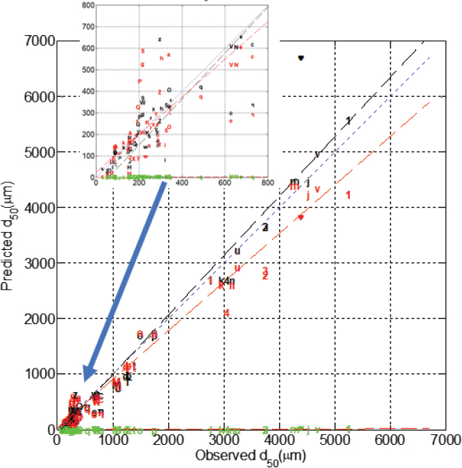
Figure D.1 compares three of the equilibrium models to the 80 experimental observations described in the last section. The figure shows that the Paris et al. (2012) model (green) underestimates droplet sizes by several orders of magnitude—consistent with the findings of Adams et al. (2013). The models of SINTEF and ASA show good predictive ability with a correlation coefficient squared of about 0.98. Both models are biased slightly low (model averages 2%-3% lower than observations). The average absolute percentage difference between model and observation for the SINTEF (Li) model is 24% (35%) with 90% confidence limits of roughly 50% (70%). However, a look at Figure D.1 shows that at times there are sizeable errors, which is reflected in the high coefficient of variation (mean/standard deviation) of ~1 for both models. These statistics become meaningless for the Paris model because predictions are an order of magnitude or more smaller than the observations.
Of particular interest is the DeepSpill field measurement (heart symbol) because it comes closest to DWH-like scales. The SINTEF model overestimates the observations by about 50% while the ASA model makes a perfect forecast. However, this perfection comes as no accident because ASA used the DeepSpill measurement to fit their model coefficients. Paris underpredicts by two orders of magnitude following the trend seen in Figure D.1 for the lab experiments. VDROP-J and Oildroplets have also been compared to DeepSpill in their respective publications and those are shown in row 2 of Table D.1.
The DeepSpill comparison for VDROP-J comes from Zhao et al. (2014) and is marked as questionable. That is because a careful reading of their paper shows that they used an optimized calibration coefficient, Kb, to calculate the 4,500 µm value. In a practical application of the model they would not be able to use an optimized fit but would have to use their Equation 33 to calculate Kb. How much difference would it make if they had used the predicted Kb instead of the best fit?
We do not know for sure without running the model again, but we can get a sense of its importance from their Figure 10 which suggests d50 = 0.5 mm, or nearly an order of magnitude less than their estimate using the best-fit Kb.1 This estimate assumes linear extrapolation which is arguable but is taken here to show that the d50 calculated from VDROP-J is quite sensitive to Kb. If VDROP-J were re-run with the predicted Kb from Equation 33 it would predict a d50 substantially smaller than observed; hence the question mark in Table D.1.
Zhao et al. (2014) used best-fit Kb’s when comparing VDROP-J to all the observations in their paper (see their Figures 6 to 13). This was a necessary first step to calibrate Kb and develop Equation 33. However, they never truly validated the predictive ability of the model by comparing it to a new set of observations using Equation 33. Though a less rigorous validation step, they could have at least compared the model to the calibration dataset using Equation 33 to calculate Kb. Had they done so they would have found the uncertainty bounds to be substantial given the sensitivity of VDROP-J’s d50 estimate to variations in Kb (see DeepSpill example in previous paragraph) coupled with the considerable uncertainty in Equation 33 (see their Figure 14). It is noteworthy that Zhao et al. (2017a) and Nissanka and Yapa (2016) repeated this same process. In summary, the two population models have been calibrated, but not truly validated.
___________________
1 Equation 33 gives Kb = 0.100 using the properties listed in their Table 1. Figure 10 shows curves for three values of Kb. The curve for Kb = 0.028 shows a d50 = 5 mm while the curve for Kb = 0.05 gives a d50 = 3.5. Using these values and assuming linear extrapolation means a Kb = 0.10 gives d50 = 0.5 mm.
TABLE D.1 The d50 in µm Predicted by Models for Both Untreated and Treated Oil During Deepwater Horizon (DWH) and Untreated Oil During DeepSpill
| Case | DOR% | SINTEFa Um | Spauldingb | ASAc | VDROP-Jd | Paris um | Oildroplets |
|---|---|---|---|---|---|---|---|
| DeepSpill | 0 | 6,700 | NA | 4,300 | 4,500? | 32 | ~4,000 |
| DWH | 0 | 5,800 | 2,600 | 10,200 | 4,200 | 190 | NA |
| DWH | 0.4 | 1,800 | 100/2,600 | 3,400 | 1,300 | 70 | NA |
| DWH | 1.0 | 530 | 200/2,600 | 740 | 140 | 10 | NA |
aCalculated using ρo = 763 kg/m3, µ = 0.7 cp, GOR = 0.4,3, σ = 24.5 cp (DOR = 0%), σ = 4.54 mN/m (0.4%), σ = 0.24mN/m (1%). Uses the SINTEF models described in Skancke et al. (2016) except that we have not accounted for temperature effects on oil viscosity.
bThese are approximate peaks taken from Figure 9 of Spaulding et al. (2017). The 0.4% DOR case in the table comes from their “Best Estimate” while the 1% comes from their “high dispersant” case. The dual peaks in the droplet size distribution arise because they have assumed only partial mixing of the dispersant.
cThese are estimates assuming oil characteristics at the surface as per Li et al. (2017). ρo = 862 kg/m3, µ = 0.74 cp, GOR = 0.4, σ = 24.5 mN/m (DOR = 0%), σ = 4.54 mN/m (0.4%), σ = 0.24 mN/m (1%).
dFrom Gros et al., 2017.
COMPARISONS BETWEEN MODELS AND DEEPWATER HORIZON OBSERVATIONS
Table D.1 also compares the models for DWH cases with different dispersant-to-oil ratios (DORs). Unfortunately, there are no direct measures of droplet size but the work of Gros et al. (2017) suggests that a d50 of about 1 mm would satisfy their observed dataset, which corresponds to 0.4% DOR. This dataset is largely based on analyzed hydrocarbon concentration measurements integrated over time and space using the hydrocarbon fractionation methodology recommended in Chapter 5. By integrating over time and normalizing the concentration data by conservative constituents they remove many of the problems one runs into by comparing to raw time series. As shown in further runs by Socolofsky and Gros commissioned by this committee (henceforth referred to as SG and shown in Appendix E), their dataset is remarkably good at discriminating between proposed droplet sizes.
The third row of Table D.1 shows the case of 0.4% DOR and indicates that both VDROP-J and the SINTEF model fall close to the 1 mm value suggested by Gros et al., thus providing some validation for those models. The value from Spaulding et al. (2017) assumes a dual-peaked droplet size distribution for the dispersed cases based on their argument that the dispersant was not thoroughly mixed. The follow-on modeling by SG does not reproduce the Gros et al. dataset well. At 3.4 mm, the ASA model is considerably larger than 1 m but SG did not make a run with 3.4 mm so we cannot say for sure how it would compare to their dataset. However, the CRA-2 study described in Chapter 6 (see Figure 6.9a) does suggest that the difference between 1 and 3.4 mm would not substantially affect degradation, evaporation, or oil in the water column implying that the ASA estimate might not compare too badly to the Gros dataset.
Table D.1 shows that the Paris model predicts a d50 of 70 µm. SG ran a case with a d50 = 115 µm for DWH and found that virtually no oil made it to the surface, and far too much oil was found subsurface. In short, the Paris result is clearly inconsistent with the Gros et al. (2017) dataset and numerous other sources such as Ryerson et al. (2012) showing substantial oil at the surface.
One noteworthy point to make is that the two droplet models (VDROP-J and SINTEF, and arguably2 ASA’s model) replicate the Gros et al. dataset and do so without including some of the complicating processes conjectured in Chapter 2 (large pressure gradients, churn flow, or tip streaming). This suggests that those processes were not substantial for DWH. That is not to say that these processes could not be important in other scenarios.
In summary, both the VDROP-J and SINTEF models indicate a d50 that compares well with what we consider to be the best available estimate of the DWH d50 available to date inferred by Gros et al. (2017). The ASA model is a bit on the high side though it would likely still compare fairly well with the Gros dataset. On the other hand, the Paris d50 is too small by an order of magnitude.
Table D.1 also shows d50 values for a 0% and 1% DOR so it is interesting to compare VDROP-J, ASA, and SINTEF for these other values even though we do not have any observations for these cases from DWH. The ratios among the three models are remarkably constant at 0% and 0.4% DOR (i.e., the SINTEF model is 1.4× of the VDROP-J value while the ASA model is near 2.5). However, that trend stops at 1% DOR where these factors more than double. In other words, VDROP-J reduces the d50 at 1% far more than the other two models. Which model is correct? There are no observations to help us but it is worth noting that VDROP-J was calibrated with only two experiments where dispersant was applied (Zhao et al., 2014, 2017a). In contrast the SINTEF and ASA models have now been compared to 33 experiments in Figure D.1 with SSDI applied.
How much do the differences in predicted droplet size between the three models affect the calculated fate? For the 0% and 0.4% DOR, the answer is probably not much. This is based on the CRA-2 study described in Chapter 6. Figure 6.9a taken from that study shows that at 1,500 m there is little change in the volumes going to evaporation and degradation for droplets greater than 1 mm. However, at 1%, Figure 6.9a shows that there is a sizable difference. For example, the SINTEF (530 µm) and ASA models (740 µm) result in a degradation of 10%-15% of the total spill volume while VDROP-J (140 µm) is 40%-50%. In short, one walks away with a very different picture of SSDI effectiveness at 1% DOR if one uses VDROP-J instead of the others.
SUMMARY
Though the five droplet models mentioned in Chapter 2 have been compared to observations by their authors, all but the SINTEF model have considered a relatively small set of about a dozen oil jet experiments. There are now roughly 200 oil jet experiments available for comparisons, mostly from Brandvik et al. (2013, 2014, 2017, 2018, 2019a,b). These experiments cover a wide range of scales and conditions—discharge diameters of 0.5 to 50 mm and flow rates of 0.2 to 400 l/min, pressure ranges of 2 to 1,500 m of water, multiple DOR values, multiple oil densities, multiple gas-to-oil ratios (GORs), and live oils. Further details are given in the last section.
We selected 80 experiments from this large set of observations and compared three equilibrium models to those. These comparisons show that both the ASA and SINTEF models compare well with a correlation coefficient squared of about 0.98 though there is considerable scatter as indicated by 90% confidence limits of up to 70%. The Paris model underestimates the observations by orders of magnitude for reasons identified in Adams et al. (2013).
Some might argue that the good performance of the ASA and SINTEF model is because they have tuned their calibration coefficients to the observations. A close look at the sequence of publications of these models shows that they based their calibration coefficients on a dozen or so observations that did not include the vast majority of the measurements in our Figure D.1.
The authors of the two population models, VDROP-J and Oildroplets, were unwilling to participate in our comparison. Given the model complexity, we could not program them within our
___________________
2 The ASA d50 for 0.4% DOR is nearly three times larger than VDROP-J, so it could reproduce the Gros et al. (2017) dataset about as well as VDROP-J especially if one used a fairly large width parameter for the droplet size distribution.
time constraints. However, we were able to gather some insights about these models from published results for DeepSpill and DWH and further runs by SG.
Comparisons with the DeepSpill experiment reveal a number of important findings. First, the SINTEF model over-predicts the droplet size by about 50% though this is not too bad in light of the uncertainty in the observations. The Paris model predicts a droplet size two orders of magnitude too low. The ASA prediction is perfect but not insightful because they calibrated to the DeepSpill measurement. Finally, the authors of the two population models claim to closely match the DeepSpill experiment, but a close look at their comparisons reveals that they optimized their calibration coefficient to achieve that fit. If they had done a blind prediction, the error would have been larger. In the case of VDROP-J, we have done an estimate that suggests it would have underestimated the droplet size by a sizable amount.
Comparisons with the DWH dataset also gives some insights in several of the droplet models. Gros et al. (2017) and follow-on modeling by SG suggest the d50 for DWH was about 1 mm. Both the VDROP-J and SINTEF models predict roughly 1.5 mm while the ASA model predicts a value about two times larger. Unfortunately, SG did not run the ASA value but a look at the CRA-2 study suggests it might still compare reasonably well to the Gros dataset. The SG results show the Paris model prediction of 0.07 mm is far too small and that the dual-peaked droplet size distribution of Spaulding et al. (2017) compares less well than the VDROP-J and SINTEF models.
We also compared the models at two other DORs (0% and 1%) for the DWH conditions and found that VDROP-J gives a much smaller droplet size than the other two models at 1% DOR. There are no observations to check which model is correct but it is worrisome that VDROP-J was calibrated with only two observations that used dispersant. Because VDROP-J suggests such a substantial decrease in droplet size from 0% to 1% DOR, it makes SSDI look a lot more appealing than do the other two models.
Finally, we need to comment on the droplet size distribution. As pointed out in Chapter 2, the equilibrium models only predict the d50 and then use a heuristic method to calculate the droplet distribution. In contrast, the population models predict both the d50 and the distribution. Furthermore, the equilibrium models redistribute droplets in bin sizes greater than the largest stable droplet size using an ad hoc approach. The authors of the equilibrium models have spent little effort validating these assumptions so this is a topic that should be investigated more thoroughly. That said, it is reassuring to note that the sensitivity studies by French-McCay and Crowley (2018) show that the ultimate fate of the oil is fairly insensitive to the details of the size distribution. It is also reassuring that the SINTEF d50 compares so well to the experimental observations because in several of those cases the modeled d50 is shifted by as much as two times by their ad hoc method of dealing with droplets exceeding the maximum stable droplet size.
CONCLUSIONS
At last we are in a position to address Task 6 of the committee Work Scope with regard to droplet models. We conclude that both the ASA and SINTEF models probably can estimate droplet sizes with confidence limits of roughly 70% for simple jets. Given their firmer physical basis, VDROP-J and Oildroplets could perform even better but this is conjecture until these models are more thoroughly calibrated and truly validated using predicted calibration coefficients. It is reassuring that the VDROP-J and SINTEF models compare well with each other and the definitive DWH dataset of Gros et al. (2017). That said, it is troubling that VDROP-J suddenly breaks with the SINTEF and ASA models at a DOR of 1% and predicts a much smaller droplet size. This discrepancy is important because fate benefits will look far more positive with VDROP-J than with the other two models.
What are the implications of this uncertainty in the droplet models? Of course, we cannot answer that for a generic site but we can gain some insights for a large blowout by looking at the results of the CRA-2 study described in Chapter 6. Figure 6.9 shows the impact of droplet size on the peak volume of the oil during a blowout in a DWH-like setting. The upper panel applies to a site in 1,400 m of water while the lower panel is set in 500 m of water. For undispersed oil, one would expect a droplet size in the multi-mm range for a large blowout in either water depth. Using our confidence limit estimate of 70% and assuming d50 = 5 mm gives a range of 1.5-8.5 mm. Looking at the upper and lower panels of Figure 6.9, this range of d50 shows that the droplet uncertainty has negligible impact on the calculated fate in either water depth. These relatively big droplets rise so quickly to the surface that it really does not matter if they are 1 mm or 8 mm. On the other hand, for dispersed oil, a reasonable droplet size might be 0.5 mm, giving a range of 0.15-0.85 mm. Referring to Figure 6.9, we now see dramatically different fates at both 500 and 1,400 m depth. For example, in 1,400 m of water, roughly 50% of the oil mass ends up in the water column with d50 = 0.15 mm; it is about half that with d50 = 0.85 mm. While the CRA-2 focused on the Gulf of Mexico, the sensitivity to errors in droplet size will likely apply to many other parts of the world.
Based on this analysis we conclude:
- The two equilibrium models from SINTEF and ASA predict 80 available observations from high-quality lab experiments with a mean error of less than 35% though with a fairly substantial scatter as reflected by the 90% confidence limits of 70%.
- The published comparisons between observations and the two population models, VDROP-J and Oildroplets, are promising but inadequate because of their limited number and their use of calibration coefficients that were optimized to fit the individual experiments. Further comparisons are needed to truly validate the models for a wide range of conditions. Once this is done, the population models are likely to outperform the equilibrium models, in part because they predict both droplet and bubble sizes; the entire size distribution, not just the d50; and the time evolution of the droplet/bubble sizes.
- Comparisons with DWH suggest both the VDROP-J and SINTEF models predict reasonable droplet sizes though the uncertainty of the observed dataset remains a question mark as does the rather low d50 predicted by VDROP-J for the 1% DOR case.
- The uncertainty in predicted d50 estimated in item 1 probably has little impact in calculating the droplet size for untreated oil in many high-volume blowout scenarios but that uncertainty can dramatically affect the modeled fate for treated (dispersed) oil. Hence, there is a demonstrable need for further research to remove uncertainty in droplet models especially for dispersed oil.
SUPPLEMENTAL INFORMATION: DESCRIPTION OF EXPERIMENTAL OBSERVATIONS
Table D.2 summarizes the experiments used in the comparisons and the attached spreadsheet documents the key properties used as model input. The first column of the spreadsheet includes a “symbol” that can be used to trace that particular experiment to Figure D.1. All of the experiments involved jetting of oil into seawater though some also included methane either as free gas or saturated in the oil (live oil). We have not included any data from stirred autoclaves as there is no evidence to suggest that these generate similar turbulence fields or droplets to a jet. Indeed, the fact that the Paris et al. (2012) model, based on autoclave measurements, underestimates observed droplets by orders of magnitude (see green symbols in Figure D.1) supports the contention of Adams et al. (2013) that autoclaves generate a very different turbulence field (and hence droplet
TABLE D.2 Summary of Observations of Droplet Size Formed by a Subsurface Jet
| Name | Facility | Press (m) | Flow (l/min) | Well Φ (mm) | Fluids | References |
|---|---|---|---|---|---|---|
| SINTEF 0 | SINTEF Tower | 5 | 0.2-5 | 0.5-3 | Oil, air, Corexit | Brandvik et al., 2013 |
| SINTEF 1 | SINTEF Tower | 5 | 1.2 | 1.5 | Oil, Corexit | Brandvik et al., 2018 |
| SINTEF 2 | SINTEF Tower | 5 | 1.2 | 1.5 | Oil, dispersant | Brandvik et al., 2014 |
| SINTEF 3 | SwRI, Sintef T. | 5-1,750 | 1.2 | 1.5 | Oil, dispersant | Brandvik et al., 2019a |
| SINTEF 5 | SwRI, Sintef T. | 5-1,750 | 1.2 | 1.5 | Live oil, gas, Corexit | Brandvik et al., 2019b |
| C-IMAGE | Hamburg autoclave | 1,500 | 1-2 | 1.5 | Oil, methane, n-dec. | Malone et al., 2018 |
| SINTEF 6 | OHMSETT | 2 | 50-400 | 25-50 | Oil, methane, Corexit | Brandvik et al., 2017 |
| DeepSpill | Norwegian Sea | 844 | 17 | 120 | Diesel, LNG | Johansen et al., 2001 |
size) than jets. There are a number of other experimental observations of jets (e.g., Belore [2014], Masutani and Adams [2000], and Zhao et al. [2017b]), but these are unsuitable for various reasons.3
The lab experiments in Table D.2 (first six entries) span a wide range of conditions including discharge orifice scales of 1.5 to 50 mm and flow rates from 0.2 to 400 L/min. Most of the experiments come from Brandvik et al. (2014, 2017, 2018, 2019a,b) who have conducted roughly 200 individual experiments since 2011. Though none of the papers by Brandvik et al. provide error estimates on their measurements, they did numerous replicates that demonstrate the consistency of their observations. We did not use all of their experiments because there were so many replicates and we had to do all data entry manually. SINTEF 0 was not included because it has been used extensively by almost all of the models to calibrate them. It is also reassuring that the experiments of Malone et al. (2018) fit the same trend line as the similar experiments from Brandvik et al. (2013, 2014).
SINTEF 0, 1, 3, and 6 have been published in peer-reviewed journals and the remaining SINTEF work is documented in technical reports that have been available to the public for several years. The unpublished reports use similar methods, facilities, and instrumentation to SINTEF 0 and 1. Note that VDROP-J, Oildroplets, and the ASA models have used several of the experiments from SINTEF 0 in their model validation efforts, an implicit acceptance of the general methodologies employed by SINTEF.
SINTEF 0, 1, and 2 consisted of roughly 10-50 individual experiments each involving the release of an oil jet into sea water in the so-called SINTEF Tower Basin, a 6 m high by 3 m diameter cylinder. Droplet sizes were measured with a Laser In Situ Scattering and Transmissiometry (LISST) array located at 2 m above the discharge orifice. Some of the experiments had a second LISST located at 4m.
SINTEF 3 focused on the effects of pressure on the droplet size of dead oil and was the precursor for SINTEF 5, which considered pressure, gas and live oil. Most of the experiments were conducted in the large high-pressure chamber at Southwest Research Institute (SwRI), which consists of a 5.8 m long cylinder with a 2.3 m diameter capable of reaching pressures of 1,750 m of water. The Silhouette Camera (Davis et al., 2017, henceforth referred to as SilCam) was used and represented a major advance over a LISST-type device because (1) it was capable of simultaneously
___________________
3 Masutani and Adams had difficulty measuring the oil droplets because of limitations with their PDPA instrument. Zhao et al. were impacted by major fractionation due to their use of a horizontal jet. Belore studied a multiphase horizontal jet of gas and oil. Fractionation was an issue for them because of the inability of their primary measurement device (Laser In Situ Scattering and Transmissiometry) to differentiate between droplets and bubbles.
measuring both droplets and bubbles of any size above a few µm, and (2) it could measure much higher concentrations than the LISST.
The other small-scale set of observations comes from Malone et al. (2018) who conducted eight experiments in a pressurized column of 99 L. Flow rates and discharge orifice size were similar to SINTEF 0, 1, and 2.
An inherent weakness with these small-scale studies is their small discharge pipe and low flow rate, which were several orders of magnitude smaller than a DWH-like spill. The smaller scale means that models calibrated with this data are extrapolating several orders of magnitude to get to field scales.
To get to larger scales, SINTEF ran two sets of replicate experiments, one in the SINTEF Tower Basin used in the earlier studies and the other in the Ohmsett flow facility using a vertical discharge pipe. They looked at flow rates and discharge orifices that were at least an order of magnitude higher than in earlier studies. While Ohmsett is 200 m long by 20 m wide, it is only 2.4 m deep so it was necessary to apply a horizontal current (0.25-1.07 m/s), simulated by towing the discharge pipe, in order to dilute the oil sufficiently to take droplet measurements. For the Tower Basin, the layout was identical to SINTEF 0-2 except that two SilCams were used instead of the LISST, and the SilCams were placed at 5 m above the discharge to allow for sufficient dilution. The introduction of SilCams into the Tower Basin allowed for much higher flow rates and droplet sizes than explored in SINTEF 0, 1, and 2.
The overriding uncertainty for the Ohmsett experiments comes from the potential for significant droplet fractionation, which is the natural consequence of the fact that the oil plume gets pushed over to the side by the horizontal current. Zhao et al. (2017b) has shown how important fractionation can be with horizontal plumes. To counter the possible effects of fractionation, SINTEF 6 did extensive calculations (Brandvik et al., 2017) to determine where to position the SilCam to ensure that it was in the center of the oil plume.
Ultimately, the importance of fractionation in the Ohmsett experiments was not a concern. There were 12 experiments that were conducted in both the Tower Basin and the Ohmsett tank; the d50s are compared in Figure D.2. The data points are color coded with red indicating questionable results (as determined by Brandvik et al., 2017) generally caused by oil clouding the limited volume of the Tower Basin. Even including these questionable data, the correlation coefficient squared is nearly 0.9. There is a slight bias with the Ohmsett d50 being 20%-30% larger than the Tower d50 at the larger d50s. That said, that bias is coming from the questionable Tower results as denoted by the red symbols. The generally good comparison between the Ohmsett and Tower observations suggests that fractionation is of modest importance in the Ohmsett data at the larger droplet sizes. Hence, SINTEF 6 represents a valuable dataset for model calibration and validation, especially because its scales are more than an order of magnitude larger than the previous measurements.
The other large-scale dataset comes from the DeepStar field experiment, which consisted of four 1-hour field experiments in which gas and gas/oil mixtures were injected through a 12 cm nozzle at a depth of 840 m off the Norwegian Coast (Johansen et al., 2001, 2003). The most relevant of these is the second release involving a mixture of natural gas and marine diesel. Droplet volume distributions were reported on pages 63 and 64 of Johansen et al. (2001) for elevations of 4-5 m, 9-10 m, 14-22 m, and 34-55 m above the discharge (designated as Cases 5-8, respectively). There is considerable scatter in these cases but no obvious correlation to measurement height so we have simply averaged the d50 from all levels.
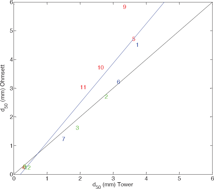
TABLE D.3 Summary of Experiments Used in Figure D.2
| Exp. Name | Pipe Φ mm | Oil Flow L/min | Temp C° | IFT mN/m | GOR m3/m3 | Oil ρ kg/m3 | Visc cp | DOR % | Source |
|---|---|---|---|---|---|---|---|---|---|
| \heartsuit | 120 | 1,000 | 4 | 25.00 | 0.50 | 854 | 3.9 | 0.0 | DeepSpill |
| \vartheta | 1.5 | 1.2 | 13 | 13.40 | 0.00 | 832 | 7.1 | 0.0 | SINTEF 2 |
| \iota | 1.5 | 1.2 | 13 | 2.30 | 0.00 | 832 | 7.1 | 1.0 | SINTEF 2 |
| \kappa | 1.5 | 1.2 | 13 | 0.01 | 0.00 | 832 | 7.1 | 2.0 | SINTEF 2 |
| \lambda | 1.5 | 1.2 | 75 | 13.40 | 0.00 | 832 | 2.8 | 0.0 | SINTEF 2 |
| \mu | 1.5 | 1.2 | 75 | 6.80 | 0.00 | 832 | 2.8 | 1.0 | SINTEF 2 |
| \nu | 1.5 | 1.2 | 75 | 0.10 | 0.00 | 832 | 2.8 | 2.0 | SINTEF 2 |
| \xi | 1.5 | 1.2 | 50 | 12.20 | 0.00 | 832 | 4.1 | 0.0 | SINTEF 2 |
| \pi | 1.5 | 1.2 | 50 | 13.10 | 0.00 | 832 | 4.1 | 1.0 | SINTEF 2 |
| \rho | 1.5 | 1.2 | 50 | 0.02 | 0.00 | 832 | 4.1 | 2.0 | SINTEF 2 |
| \sigma | 1.5 | 1.2 | 23 | 17.50 | 0.00 | 832 | 6.0 | 0.0 | SINTEF 2 |
| \varsigma | 1.5 | 1.2 | 23 | 1.90 | 0.00 | 832 | 6.0 | 1.0 | SINTEF 2 |
| \tau | 1.5 | 1.2 | 23 | 0.01 | 0.00 | 832 | 6.0 | 2.0 | SINTEF 2 |
| \phi | 1.5 | 1.2 | 18 | 10.00 | 0.00 | 900 | 20.0 | 0.0 | SINTEF 2 |
| \psi | 1.5 | 1.2 | 18 | 3.50 | 0.00 | 900 | 20.0 | 1.0 | SINTEF 2 |
| A | 1.5 | 1.2 | 78 | 10.70 | 0.00 | 900 | 20.0 | 0.0 | SINTEF 2 |
| B | 1.5 | 1.2 | 85 | 3.70 | 0.00 | 900 | 20.0 | 1.0 | SINTEF 2 |
| C | 1.5 | 1.2 | 13 | 15.00 | 0.00 | 797 | 4.0 | 0.0 | SINTEF 2 |
| D | 1.5 | 1.2 | 13 | 0.06 | 0.00 | 797 | 4.0 | 2.0 | SINTEF 2 |
| E | 0.5 | 0.2 | 13 | 15.50 | 0.00 | 839 | 10.0 | 0.0 | SINTEF 1 |
| F | 1.5 | 1.0 | 13 | 15.50 | 0.00 | 839 | 10.0 | 0.0 | SINTEF 1 |
| G | 1.5 | 1.5 | 13 | 15.50 | 0.00 | 839 | 10.0 | 0.0 | SINTEF 1 |
| H | 1.5 | 1.5 | 13 | 0.05 | 0.00 | 839 | 10.0 | 2.0 | SINTEF 1 |
| I | 1.5 | 1.5 | 13 | 0.09 | 0.00 | 839 | 10.0 | 4.0 | SINTEF 1 |
| J | 2.0 | 5.0 | 13 | 15.50 | 0.00 | 839 | 10.0 | 0.0 | SINTEF 1 |
| K | 3.0 | 5.0 | 13 | 15.50 | 0.00 | 839 | 10.0 | 0.0 | SINTEF 1 |
| L | 3.0 | 1.5 | 22 | 19.30 | 0.00 | 700 | 0.9 | 0.0 | SINTEF 5 |
| M | 3.0 | 1.5 | 26 | 18.20 | 0.23 | 700 | 0.8 | 0.0 | SINTEF 5 |
| N | 3.0 | 1.5 | 27 | 18.20 | 1.00 | 706 | 0.8 | 0.0 | SINTEF 5 |
| O | 3.0 | 1.5 | 28 | 21.60 | 3.67 | 705 | 0.8 | 0.0 | SINTEF 5 |
| P | 3.0 | 1.5 | 28 | 2.80 | 0.17 | 695 | 0.8 | 1.0 | SINTEF 5 |
| Q | 3.0 | 1.5 | 32 | 3.27 | 0.67 | 695 | 0.7 | 1.0 | SINTEF 5 |
| R | 3.0 | 1.5 | 36 | 3.87 | 2.33 | 690 | 0.7 | 1.0 | SINTEF 5 |
| S | 3.0 | 1.5 | 27 | 3.87 | 0.00 | 700 | 0.8 | 1.0 | SINTEF 5 |
| T | 3.0 | 1.5 | 27 | 18.60 | 0.00 | 776 | 0.8 | 0.0 | SINTEF 5 |
| U | 3.0 | 1.5 | 37 | 21.00 | 0.43 | 774 | 0.7 | 0.0 | SINTEF 5 |
| V | 3.0 | 1.5 | 36 | 21.50 | 1.13 | 773 | 0.7 | 0.0 | SINTEF 5 |
| W | 3.0 | 1.5 | 49 | 19.50 | 4.00 | 773 | 0.6 | 0.0 | SINTEF 5 |
| X | 3.0 | 1.5 | 50 | 1.77 | 3.93 | 772 | 0.5 | 1.0 | SINTEF 5 |
| Y | 3.0 | 1.5 | 45 | 3.37 | 0.87 | 772 | 0.6 | 1.0 | SINTEF 5 |
| Z | 3.0 | 1.5 | 41 | 3.37 | 0.40 | 773 | 0.6 | 1.0 | SINTEF 5 |
| a | 3.0 | 1.5 | 40 | 3.57 | 0.00 | 773 | 0.6 | 1.0 | SINTEF 5 |
| b | 3.0 | 1.5 | 22 | 22.00 | 0.00 | 764 | 0.8 | 0.0 | SINTEF 5 |
| c | 3.0 | 1.5 | 30 | 20.00 | 0.93 | 773 | 0.7 | 0.0 | SINTEF 5 |
| d | 3.0 | 1.5 | 31 | 21.30 | 0.00 | 775 | 0.7 | 0.0 | SINTEF 5 |
| e | 3.0 | 1.5 | 34 | 20.00 | 0.80 | 755 | 0.6 | 0.0 | SINTEF 5 |
| f | 3.0 | 1.5 | 38 | 2.87 | 1.00 | 753 | 0.6 | 1.0 | SINTEF 5 |
| g | 3.0 | 1.5 | 39 | 2.87 | 0.00 | 754 | 0.5 | 1.0 | SINTEF 5 |
| h | 3.0 | 1.5 | 35 | 3.27 | 0.00 | 752 | 0.6 | 1.0 | SINTEF 5 |
| i | 3.0 | 1.5 | 37 | 0.57 | 0.87 | 770 | 0.6 | 1.0 | SINTEF 5 |
| j | 25.0 | 50.0 | 13 | 20.00 | 0.00 | 826 | 4.6 | 0.0 | SINTEF 6 |
| k | 25.0 | 80.0 | 13 | 20.00 | 0.00 | 826 | 4.6 | 0.0 | SINTEF 6 |
| Exp. Name | Pipe Φ mm | Oil Flow L/min | Temp C° | IFT mN/m | GOR m3/m3 | Oil ρ kg/m3 | Visc cp | DOR % | Source |
|---|---|---|---|---|---|---|---|---|---|
| l | 25.0 | 80.0 | 4 | 20.00 | 0.00 | 826 | 5.1 | 0.0 | SINTEF 6 |
| m | 25.0 | 50.0 | 5 | 20.00 | 0.00 | 826 | 5.0 | 0.0 | SINTEF 6 |
| n | 25.0 | 80.0 | 5 | 20.00 | 0.00 | 826 | 5.0 | 0.0 | SINTEF 6 |
| o | 25.0 | 120.0 | 6 | 20.00 | 0.00 | 826 | 5.0 | 0.0 | SINTEF 6 |
| p | 25.0 | 120.0 | 6 | 20.00 | 0.00 | 826 | 4.9 | 0.0 | SINTEF 6 |
| q | 25.0 | 50.0 | 5 | 0.20 | 0.00 | 826 | 5.0 | 1.0 | SINTEF 6 |
| r | 25.0 | 80.0 | 5 | 0.20 | 0.00 | 826 | 5.0 | 1.0 | SINTEF 6 |
| s | 25.0 | 120.0 | 6 | 0.20 | 0.00 | 826 | 5.0 | 1.0 | SINTEF 6 |
| t | 32.0 | 300.0 | 6 | 20.00 | 0.00 | 826 | 4.9 | 0.0 | SINTEF 6 |
| u | 32.0 | 120.0 | 13 | 20.00 | 0.00 | 826 | 4.6 | 0.0 | SINTEF 6 |
| v | 32.0 | 80.0 | 13 | 20.00 | 0.00 | 826 | 4.6 | 0.0 | SINTEF 6 |
| w | 32.0 | 300.0 | 5 | 0.20 | 0.00 | 826 | 5.0 | 1.0 | SINTEF 6 |
| x | 32.0 | 120.0 | 7 | 0.20 | 0.00 | 826 | 4.9 | 1.0 | SINTEF 6 |
| y | 32.0 | 120.0 | 7 | 0.02 | 0.00 | 826 | 4.9 | 2.0 | SINTEF 6 |
| z | 32.0 | 120.0 | 3 | 0.20 | 0.00 | 826 | 20.0 | 1.0 | SINTEF 6 |
| 1 | 50.0 | 200.0 | 13 | 20.00 | 0.00 | 826 | 4.6 | 0.0 | SINTEF 6 |
| 2 | 50.0 | 300.0 | 13 | 20.00 | 0.00 | 826 | 4.6 | 0.0 | SINTEF 6 |
| 3 | 50.0 | 300.0 | 7 | 20.00 | 0.00 | 826 | 4.9 | 0.0 | SINTEF 6 |
| 4 | 50.0 | 400.0 | 7 | 20.00 | 0.00 | 826 | 4.9 | 0.0 | SINTEF 6 |
| 5 | 50.0 | 300.0 | 15 | 0.20 | 0.00 | 826 | 4.2 | 1.0 | SINTEF 6 |
| \alpha | 1.5 | 2.1 | 20 | 22.00 | 0.00 | 864 | 15.7 | 0.0 | Malone 1.1 |
| \beta | 1.5 | 2.1 | 20 | 22.00 | 0.00 | 864 | 15.7 | 0.0 | Malone 1.2 |
| \gamma | 1.5 | 2.0 | 20 | 32.00 | 0.00 | 817 | 1.3 | 0.0 | Malone 2.1 |
| \delta | 1.5 | 2.1 | 20 | 32.00 | 0.00 | 817 | 1.30 | 0.0 | Malone 2.2 |
| \epsilon | 1.5 | 1.1 | 20 | 55.00 | 0.00 | 741 | 1.10 | 0.0 | Malone 3.1 |
| \zeta | 1.5 | 1.2 | 20 | 55.00 | 0.00 | 741 | 1.10 | 0.0 | Malone 3.2 |
| \eta | 1.5 | 1.1 | 20 | 44.00 | 0.00 | 662 | 0.39 | 0.0 | Malone 4.1 |
| \theta | 1.5 | 1.2 | 20 | 44.00 | 0.00 | 662 | 0.39 | 0.0 | Malone 4.2 |
REFERENCES
Adams, E. E., S. A. Socolofsky, and M. Boufadel. 2013. Comment on “Evolution of the Macondo well blowout: Simulating the effects of the circulation and synthetic dispersants on the subsea oil transport.” Environmental Science & Technology 47(20):11905.
Belore, R. 2014. Subsea chemical dispersant research. In Proceedings of the 37th Arctic and Marine Oilspill Program Technical Seminar on Environmental Contamination and Response. Canmore, Alberta, Canada: Environment Canada. Pp. 618-650.
Boxall, J. A., C. A. Koh, E. D. Sloan, A. K. Sum, and D. T. Wu. 2012. Droplet size scaling of water-in-oil emulsions under turbulent flow. Langmuir 28(1):104-110.
Brandvik, P. J., Ø. Johansen, F. Leirvik, U. Farooq, and P. S. Daling. 2013. Droplet breakup in subsurface oil releases—Part 1: Experimental study of droplet breakup and effectiveness of dispersant injection. Marine Pollution Bulletin 73(1):319-326. DOI: 10.1016/j.marpolbul.2013.05.020.
Brandvik, P. J., Ø. Johansen, U. Farooq, E. Davies, D. Krause, and F. Leirvik. 2014. Sub-Surface Oil Releases—Experimental Study of Droplet Distributions. Phase II, SINTEF Report 102001616, unrestricted distribution. Trondheim, Norway: SINTEF.
Brandvik, P. J., E. Davies, Ø. Johansen, F. Leirvik, and R. Belore. 2017. Subsea Dispersant Injection—Large-Scale Experiments to Improve Algorithms for Initial Droplet Formation (Modified Weber Scaling). SINTEF Report OC2017 A-087, unrestricted distribution. Trondheim, Norway: SINTEF.
Brandvik, P. J., Ø. Johansen, F. Leirvik, D. F. Krause, and P. S. Daling. 2018. Subsea dispersants injection (SSDI), effectiveness of different dispersant injection techniques—An experimental approach. Marine Pollution Bulletin 136:385-393. DOI: 10.1016/j.marpolbul.2018.09.021.
Brandvik, P. J., C. Storey, E. J. Davies, and F. Lervik. 2019a. Quantification of oil droplets under high pressure laboratory experiments simulating deep water oil releases and subsea dispersants injection (SSDI). Marine Pollution Bulletin 138:520-525. DOI: 10.1016/j.marpolbul.2018.11.020.
Brandvik, P. J., C. Storey, E. J. Davies, and Ø. Johansen. 2019b. Combined releases of oil and gas under pressure: The influence of live oil and natural gas on initial oil droplet formation. Marine Pollution Bulletin 140:485-492. DOI: 10.1016/j.marpolbul.2019.01.036.
Davis, E. J., D. A. E. Engelbertha Dunnebier, O. Johansen, P. J. Brandvik, S. Masutani, and I. Nagamine. 2017. Shedding from Chemically-Treated Oil Droplets Rising in Sea Water. Unrestricted distribution. Trondheim, Norway: SINTEF.
French-McCay, D., and D. Crowley. 2018. Sensitivity Analysis for Oil Fate and Exposure Modeling of a Subsea Blowout—Data Report. Washington, DC: American Petroleum Institute.
Gros, J., S. A. Socolofsky, A. L. Dissanayake, I. Jun, L. Zhao, M. C. Boufadel, C. M. Reddy, and J. S. Arey. 2017. Petroleum dynamics in the sea and influence of subsea dispersant injection during Deepwater Horizon. Proceedings of the National Academy of Sciences of the United States of America 114(38):10065-10070.
Johansen, Ø., H. Rye, A. G. Melbye, H. V. Jensen, B. Serigstad, and T. Knutsen. 2001. DeepSpill JIP—Experimental Discharges of Gas and Oil at Helland Hansen—June 2000. Technical Report, DeepSpill JIP, Report No. STF66 F01082. Trondheim, Norway: SINTEF.
Johansen, Ø., H. Rye, and C. Cooper. 2003. DeepSpill—Field study of a simulated oil and gas blowout in deep water. Spill Science and Technology Bulletin 8(5-6):433-443. DOI: 10.1016/S1353-2561(02)00123-8.
Johansen, Ø., P. J. Brandvik, and U. Farooq. 2013. Droplet breakup in subsea oil releases—Part 2: Prediction of droplet size distributions with and without injection of chemical dispersants. Marine Pollution Bulletin 73:327-335.
Li, Z., M. Spaulding, D. French-McCay, D. Crowley, and J. R. Payne. 2017. Development of a unified oil droplet size distribution model with application to surface breaking waves and subsea blowout releases considering dispersant effects. Marine Pollution Bulletin 114(1):247-257. DOI: 10.1016/j.marpolbul.2016.09.008.
Malone, K., S. Pesch, M. Schluter, and D. Krause. 2018. Oil droplet size distributions in deep-sea blowouts: Influence of pressure and dissolved gases. Environmental Science & Technology 52(11):6326-6333. DOI: 10.1021/acs.est.8b00587.
Masutani, S. M., and E. E. Adams. 2000. Experimental Study of Multiphase Plumes and Application to Deep Ocean Oil Spills. Final report to the U.S. Department of the Interior, Minerals Management Service, contract No. 1435-01-98-CT-30946. Herndon, VA: U.S. Department of the Interior.
Nissanka, I. D., and P. D. Yapa. 2016. Calculation of oil droplet size distribution in an underwater oil well blowout. Journal of Hydraulic Research 54(3):307-320.
NRC (National Research Council). 2003. Oil in the Sea III: Inputs, Fates, and Effects. Washington, DC: The National Academies Press.
Paris, C. B., M. L. Hénaff, Z. M. Aman, A. Subramaniam, J. Helgers, D. P. Wang, V. H. Kourafalou, and A. Srinivasan. 2012. Evolution of the Macondo well blowout: Simulating the effects of the circulation and synthetic dispersants on the subsea oil transport. Environmental Science and Technology 46(24):13293-13302. DOI: 10.1021/es303197h.
Ryerson, T. B., R. Camilli, J. D. Kessler, E. B. Kujawinski, C. M. Reddy, D. L. Valentine, E. Atlas, D. R. Blake, J. de Gouw, S. Meinardi, D. D. Parrish, J. Peischl, J. S. Seewald, and C. Warneke. 2012. Chemical data quantify Deepwater Horizon hydrocarbon flow rate and environmental distribution. Proceedings of the National Academy of Sciences of the United States of America 109(50):20246-20253. DOI: 10.1073/pnas.1110564109.
Skancke, J., O. Johansen, P. J. Brandvik, and O. G. Brakstad. 2016. Implementing new features in OSCAR; Oil temperature and viscosity during droplet formation and area specific biodegradation. Report A27807, unrestricted access. Trondheim, Norway: SINTEF.
Spaulding, M., Z. Li, D. Mendelsohn, D. Crowley, D. French-McCay, and A. Bird. 2017. Application of an integrated blowout model system, OILMAP DEEP, to the Deepwater Horizon (DWH) Spill. Marine Pollution Bulletin 120(1-2):37-50. DOI: 10.1016/j.marpolbul.2017.04.043.
Zhao, L., M. C. Boufadel, S. A. Socolofsky, E. Adams, T. King, and K. Lee. 2014. Evolution of droplets in subsea oil and gas blowouts: Development and validation of the numerical model VDROP-J. Marine Pollution Bulletin 83(1):58-69. DOI: 10.1016/j.marpolbul.2014.04.020.
Zhao, L., M. C. Boufadel, T. King, B. Robinson, P. Gao, S. A. Socolfosky, and K. Lee. 2017a. Droplet and bubble formation of combined oil and gas releases in subsea blowouts. Marine Pollution Bulletin 120(1-2):203-216. DOI: 10.1016/j. marpolbul.2017.05.010.
Zhao, L., F. Gao, M. C. Boufadel, T. King, B. Robinson, K. Lee, and R. Conmy. 2017b. Oil jet with dispersant: Macro-scale hydrodynamics and tip streaming. AIChE Journal 63(11):5222-5234. DOI: 10.1002/aic.15864.


