


Below is the uncorrected machine-read text of this chapter, intended to provide our own search engines and external engines with highly rich, chapter-representative searchable text of each book. Because it is UNCORRECTED material, please consider the following text as a useful but insufficient proxy for the authoritative book pages.
NCHRP 17-65 Improved Analysis of Two-Lane Highway Capacity and Operational Performance Final Report 106 Appendices Table of Contents A. CURRENT AGENCY PRACTICES AND PREFERENCES ................................................... 115 A.1. SURVEY INSTRUMENT .................................................................................................................. 115 A.2. SURVEY RESPONSES..................................................................................................................... 127 A.3. SURVEY RESULTS......................................................................................................................... 127 A.4. SUMMARY OF FINDINGS ............................................................................................................... 133 B. SERVICE MEASURE EVALUATION ....................................................................................... 135 B.1. INTRODUCTION ............................................................................................................................ 135 B.2. HIGHWAY CAPACITY MANUAL PERFORMANCE MEASURES ....................................................... 135 B.3. ALTERNATIVE PERFORMANCE MEASURES .................................................................................. 136 B.4. PRELIMINARY ASSESSMENT OF PROPOSED PERFORMANCE MEASURES ..................................... 140 B.5. EMPIRICAL ANALYSIS OF FIELD DATA ........................................................................................ 143 B.6. SUMMARY .................................................................................................................................... 165 C. IDENTIFICATION OF VIABLE SIMULATION TOOLS FOR THE ANALYSIS OF TWO- LANE HIGHWAYS ................................................................................................................................ 175 C.1. INTRODUCTION ............................................................................................................................ 175 C.2. IDENTIFICATION OF CANDIDATE SIMULATION TOOLS ................................................................ 175 C.3. EVALUATION OF CANDIDATE SIMULATION TOOLS ..................................................................... 175 C.4. SIMULATION TOOL RECOMMENDATION ...................................................................................... 178 C.5. SWASHSIM DESCRIPTION ............................................................................................................. 178 C.6. TRANSMODELER DESCRIPTION ................................................................................................... 180 D. MODELING SPEEDS OF HEAVY VEHICLES FOR SIMULATION ................................... 183 D.1. SPEEDS ON TANGENTS ................................................................................................................. 183 D.2. SPEED ON CURVES ....................................................................................................................... 185 D.3. ACCELERATION/DECELERATION IN TANGENT-CURVE TRANSITION AREAS ............................... 188 D.4. MODELS IMPLEMENTED INTO SIMULATION TOOL ....................................................................... 189 D.5. SIMULATION EXPERIMENTAL DESIGN ......................................................................................... 207 E. APPROACH FOR ESTIMATING FOLLOWER STATUS ..................................................... 237 E.1. EVALUATION OF CATBAGAN AND NAKAMURA METHOD............................................................ 237 E.2. FOLLOWING STATUS ON TWO-LANE HIGHWAYS ........................................................................ 247 F. ANALYSIS METHODOLOGY MODEL DEVELOPMENT ................................................... 259 F.1. ESTIMATION OF FREE-FLOW SPEED ............................................................................................. 259 F.2. MODELS FOR ESTIMATION OF AVERAGE SPEED .......................................................................... 268 F.3. MODELS FOR ESTIMATION OF PERCENT FOLLOWERS.................................................................. 285 F.4. PASSING LANES ............................................................................................................................ 288 F.5. â2+1â SECTIONS ........................................................................................................................... 316 F.6. LEVEL OF SERVICE ....................................................................................................................... 330
NCHRP 17-65 Improved Analysis of Two-Lane Highway Capacity and Operational Performance Final Report 107 H. FIELD DATA COLLECTION SUPPLEMENTAL MATERIAL ............................................ 334 INTRODUCTION ..................................................................................................................................... 334 FIELD DATA SITES SUMMARY .............................................................................................................. 334 NORTH CAROLINA SITES SUMMARY .................................................................................................... 335 OREGON SITES SUMMARY .................................................................................................................... 345 MONTANA, IDAHO SITES SUMMARY .................................................................................................... 353 CALIFORNIA SITE SUMMARY ................................................................................................................ 357 DATA PROCESSING ............................................................................................................................... 359 DETECTOR DATA FOR NORTH CAROLINA AND OREGON SITES ............................................................ 364 I. SIMULATION TOOLS SUPPLEMENTAL MATERIAL ........................................................ 532 DEVELOPING A TWO-LANE HIGHWAY SIMULATION IN SWASHSIM ..................................................... 532 DEVELOPING A TWO-LANE HIGHWAY SIMULATION IN TRANSMODELER ........................................... 544 SIMULATION CALIBRATION .................................................................................................................. 562 COMPARISON OF DETECTOR FIELD DATA AND CALIBRATED SIMULATION DETECTOR DATA ............ 581 COMPARISONS OF SIMULATION DATA AND DEVELOPED MODELS FOR AVERAGE SPEED AND PERCENT FOLLOWERS ..................................................................................................................................... 652
NCHRP 17-65 Improved Analysis of Two-Lane Highway Capacity and Operational Performance Final Report 108 List of Tables Table A-1. Average Ranking Score for Performance Measures ................................................ 132 Table B-1. Preliminary assessment matrix of performance measures on two-lane highways ... 142 Table B-2. Description of Field Data at Study Sites .................................................................. 147 Table B-3. Correlation analysis results for the combined data (10873 observations) ............... 156 Table B-4. Correlation analysis results for Class I data (7114 observations) ............................ 157 Table B-5. Correlation analysis results for Class II data (1465 observations) .......................... 158 Table B-6. Correlation analysis results for Class III data (2294 observations) ......................... 159 Table B-7. Results from Multivariate Linear Regression Analysis for combined data ............. 160 Table B-8. Results from Multivariate Linear Regression Analysis for class I sites .................. 161 Table B-9. Results from Multivariate Linear Regression Analysis for class II sites ................. 161 Table B-10. Results from Multivariate Linear Regression Analysis for class III sites ............. 162 Table B-11. Performance measures ranking for combined data using R2 ................................. 162 Table B-12. Performance measures rank by class using R2 ....................................................... 163 Table B-13. Performance measures rank by site using R2 ......................................................... 163 Table B-14. Number of times variable found significant using site specific regression runs ... 164 Table B-15. Number of times variable found significant using class regression runs .............. 164 Table D-1. Desired Speed Proportions for Heavy Vehicles ...................................................... 190 Table D-2. Upgrade Speed Model Coefficients for a Single-Unit Truck. ................................. 194 Table D-3. Upgrade Speed Model Coefficients for an Intermediate Semi-Trailer Truck. ........ 194 Table D-4. Upgrade Speed Model Coefficients for an Interstate Semi-Trailer Truck. ............. 195 Table D-5. Additional Segment Lengths for Different Initial Speeds for a Single-Unit Truck. 198 Table D-6. Additional Segment Lengths for Different Initial Speeds for an Intermediate Semi- Trailer Truck. ........................................................................................................................ 198 Table D-7. Additional Segment Lengths for Different Initial Speeds for an Interstate Semi-Trailer Truck. .................................................................................................................................... 199 Table D-8. Crawl Speeds and Corresponding Segment Lengths for a Single-Unit Truck. ....... 199 Table D-9. Crawl Speeds and Corresponding Segment Lengths for an Intermediate Semi-Trailer Truck. .................................................................................................................................... 200 Table D-10. Crawl Speeds and Corresponding Segment Lengths for an Interstate Semi-Trailer Truck. .................................................................................................................................... 200 Table D-11. Heavy Vehicle Curve Speeds with a Tangent FFS of 50 mi/h .............................. 205 Table D-12. Maximum Flow Rates for Passing Lane Segments. .............................................. 217 Table D-13. Range of Variables Used in Experimental Design ................................................ 235 Table D-14. Directional Flow Rate Values for Varying Heavy Vehicle Percentages and Vertical Alignment Classifications (Passing Lane Segments) ........................................................... 236 Table E-1. Description of field data at study site ....................................................................... 243 Table E-2. Results from Multivariate Linear Regression Analysis ........................................... 246 Table E-3. Description of Field Data at Study Sites .................................................................. 249 Table E-4. Percentage of Headways with Relative Speed between the Following and Lead Vehicles of up to ±1 mi/h for ATR 8 .................................................................................... 253 Table E-5. Calculations for Estimating # of Followers in Transition Range at ATR 32 ........... 256 Table E-6. Headway Cut-off Value for Calculating Percent Followers .................................... 257 Table F-1. Coefficients for FFS-HV% Slope Model (Used in Equation (F-2) .......................... 265
NCHRP 17-65 Improved Analysis of Two-Lane Highway Capacity and Operational Performance Final Report 109 Table F-2. Coefficients Used in Speed-Flow Slope Model (Equation (F-4)) for Passing Zone and Passing Constrained Segments ............................................................................................. 273 Table F-3. Coefficients Used in Speed-Flow Slope Model (Equation (F-4)) for Passing Lane Segments ............................................................................................................................... 273 Table F-4. Coefficients Used to Calculate b3 (Equation (F-5)) for Passing Zone and Passing Constrained Segments ........................................................................................................... 274 Table F-5. Coefficients Used to Calculate b3 (Equation (F-5)) for Passing Lane Segments .... 274 Table F-6. Coefficients Used to Calculate b4 (Equation (F-6)) for Passing Zone and Passing Constrained Segments ........................................................................................................... 274 Table F-7. Coefficients Used to Calculate b4 (Equation (F-6)) for Passing Lane Segments .... 275 Table F-8. Coefficients Used in Speed-Flow Slope Model (Equation (F-8)) for Passing Zone and Passing Constrained Segments ............................................................................................. 284 Table F-9. Coefficients Used in Speed-Flow Slope Model (Equation (F-8)) for Passing Lane Segments ............................................................................................................................... 284 Table F-10. Coefficient Values for Equation (F-10) ................................................................. 285 Table F-11. Coefficient Values for Equation (F-11) ................................................................. 286 Table F-12. Coefficient Values for Equation (F-12) ................................................................. 286 Table F-13. Coefficient Values for Equation (F-13) ................................................................. 287 Table F-14. Coefficient Values for Equation (F-14) ................................................................. 287 Table F-15. Coefficient Values for Equation (F-15) ................................................................. 287 Table F-16. Effective Length of Passing Lane .......................................................................... 290 Table F-17. Description of Study Sites ...................................................................................... 291 Table F-18. Traffic Simulation Output and Deviations from Field Measurements (Calibration) ............................................................................................................................................... 295 Table F-19. Traffic Simulation Output and Deviations from Field Measurements (Validation) ............................................................................................................................................... 296 Table F-20. Effective Length of Passing Lane Using Empirical Method (miles) ..................... 299 Table F-21. Regression Results for Effective Length ................................................................ 299 Table F-22. Optimal Length of Passing Lanes .......................................................................... 302 Table F-23. Description of Field Data at Study Sites ................................................................ 304 Table F-24. Traffic Simulation Output and Deviations from Field Measurements (Calibration) ............................................................................................................................................... 307 Table F-25. Traffic Simulation Output and Deviations from Field Measurements (Validation) ............................................................................................................................................... 308 Table F-26. Percent Reduction in PF to Length of Passing Lane (Harwood Approach) ........... 310 Table F-27. Percent Reduction in PF (Proposed Approach) ...................................................... 313 Table F-28. Lengths of Passing Lane Derived Using the Proposed Approach and for Various PF Reductions............................................................................................................................. 313 Table F-29. TxDOT Recommended Passing Lane Length and Distance .................................. 324 Table F-30. Ranges and Levels for Study Variables ................................................................. 327 Table F-31. Experimental Design Test Facility Characteristics ................................................ 327 Table F-32. HCM 2010 Analysis Methodology LOS Threshold Values .................................. 330 Table F-33. HCM 2010 Methodology Experimental Design Results ........................................ 332 Table F-34. NCHRP 17-65 Methodology Experimental Design Results .................................. 332 Table F-35. Follower Density Thresholds ................................................................................. 332
NCHRP 17-65 Improved Analysis of Two-Lane Highway Capacity and Operational Performance Final Report 110 List of Figures Figure A-1. Agency Survey on Performance Measures ......................................................................... 117 Figure A-2. Survey participating agencies in the U.S. and Canada (in gray) ........................................ 127 Figure A-3. Performance measures used in two-lane highway operational analysis ............................ 128 Figure A-4. Traffic data collected by highway agencies for assessing performance ............................ 129 Figure A-5. Average ranking for characteristics of performance measures .......................................... 130 Figure A-6. Average ranking score of traffic flow aspects ..................................................................... 131 Figure B-1. Montana data collection sites ................................................................................................ 148 Figure B-2. Idaho data collection sites ..................................................................................................... 148 Figure B-3. Oregon data collection sites .................................................................................................. 149 Figure B-4. North Carolina data collection sites ...................................................................................... 149 Figure B-5. Scatterplots of performance measures vs combined flow................................................... 152 Figure B-6. Scatterplots of performance measures vs traffic split .......................................................... 153 Figure B-7. Scatterplots of performance measures vs speed variance ................................................... 154 Figure B-8. Scatterplots of performance measures vs percent heavy vehicles ...................................... 155 Figure C-1. SwashSim opening screen .................................................................................................... 179 Figure C-2. SwashSim network data entry screen ................................................................................... 180 Figure C-3. SwashSim animation screen ................................................................................................. 180 Figure C-4. TransModeler opening screen............................................................................................... 181 Figure C-5. TransModeler network coding screen (1) ............................................................................ 182 Figure C-6. TransModeler network coding screen (2) ............................................................................ 182 Figure D-1. Upgrade speed versus distance curves for a single-unit truck ............................................ 192 Figure D-2. Upgrade speed versus distance curves for an intermediate semi-trailer truck ................... 192 Figure D-3. Upgrade speed versus distance curves for an interstate semi-trailer truck ........................ 193 Figure D-4. Upgrade speed versus distance functions for an interstate semi-trailer truck .................... 196 Figure D-5. 85th percentile curve speeds of heavy vehicles entering from a tangent with an 85th percentile speed equal to 70 mi/h ......................................................................................................................... 202 Figure D-6. 85th percentile curve speeds of heavy vehicles entering from a tangent with an 85th percentile speed equal to 60 mi/h ......................................................................................................................... 202 Figure D-7. 85th percentile curve speeds of heavy vehicles entering from a tangent with an 85th percentile speed equal to 50 mi/h ......................................................................................................................... 203 Figure D-8. Performance measures versus warm-up segment length. A-C) Flow rate equals 600 veh/h. D-F) Flow rate equals 1200 veh/h. ...................................................................................................... 208 Figure D-9. Performance measure-flow relationships for 65 mi/h FFS, 3 percent grade, 1.50 mi passing constrained segment. A-C) Base simulation duration andreplications. D-F) Reduced simulation duration and replications. ..................................................................................................................... 210 Figure D-10. Performance measure-flow relationships for 65 mi/h FFS, 3 percent grade, 1.50 mi passing zone segment with 10 percent heavy vehicles in the analysis and opposing directions. A-C) Base simulation duration and replications. D-F) Reduced simulation duration and replications. .......... 211 Figure D-11. Performance measure-flow relationships for 65 mi/h FFS, 3 percent grade, 1.50 mi passing lane segment. A-C) Base simulation duration and replications. D-F) Reduced simulation duration and replications. .................................................................................................................................... 212 Figure D-12. Speed-flow curves for passing zone with 10 percent heavy vehicles in analysis direction. A) 0 percent opposing heavy vehicles. B) 10 percent opposing heavy vehicles. C) 25 percent opposing heavy vehicles. ..................................................................................................................... 214
NCHRP 17-65 Improved Analysis of Two-Lane Highway Capacity and Operational Performance Final Report 111 Figure D-13. Percent follower-flow curves for passing zone with 10 percent heavy vehicles in analysis direction. A) 0 percent opposing heavy vehicles. B) 10 percent opposing heavy vehicles. C) 25 percent opposing heavy vehicles. ........................................................................................................ 214 Figure D-14. Follower density-flow curves for passing zone with 10 percent heavy vehicles in analysis direction. A) 0 percent opposing heavy vehicles. B) 10 percent opposing heavy vehicles. C) 25 percent opposing heavy vehicles. ........................................................................................................ 215 Figure D-15. Speed-flow curves for passing zone with 10 percent heavy vehicles in analysis and opposing directions. A) Passing allowed in analysis direction only (Figure D-12B). B) Passing allowed in both directions. ................................................................................................................... 215 Figure D-16. Percent follower-flow curves for passing zone with 10 percent heavy vehicles in analysis and opposing directions. A) Passing allowed in analysis direction only (Figure D-13B). B) Passing allowed in both directions. ................................................................................................................... 216 Figure D-17. Follower density-flow curves for passing zone with 10 percent heavy vehicles in analysis and opposing directions. A) Passing allowed in analysis direction only (Figure D-14B). B) Passing allowed in both directions. ................................................................................................................... 216 Figure D-18. Performance measure-flow relationships for a vertical class 1, passing constrained segment. A-C) 1 percent, 0.50 mi grade. D-F) â3 percent, 0.50 mi grade. ...................................... 220 Figure D-19. Performance measure-flow relationships for a vertical class 3, passing zone segment with 10 percent heavy vehicles in the analysis and opposing directions. A-C) 4 percent, 0.50 mi grade. D- F) â4 percent, 0.50 mi grade. ............................................................................................................... 221 Figure D-20. Performance measure-flow relationships for a vertical class 5, passing lane segment. A-C) 7 percent, 3.00 mi grade. D-F) â7 percent, 3.00 mi grade. ............................................................... 222 Figure D-21. Performance measure-flow relationships for a vertical class 2, passing constrained segment. A-C) 3 percent, 2.00 mi grade. D-F) â3 percent, 2.00 mi grade. ...................................... 223 Figure D-22. Performance measure-flow relationships for a vertical class 3, passing constrained segment. A-C) 4 percent, 1.00 mi grade. D-F) â4 percent, 1.00 mi grade. ...................................... 224 Figure D-23. Performance measure-flow relationships for a vertical class 4, passing constrained segment. A-C) 5 percent, 1.50 mi grade. D-F) â4 percent,1.50 mi grade. ....................................... 225 Figure D-24. Performance measure-flow relationships for a vertical class 5, passing constrained segment. A-C) 7 percent, 2.00 mi grade. D-F) â7 percent, 2.00 mi grade. ...................................... 226 Figure D-25. Performance measure-flow relationships for a vertical class 1, passing zone segment with 10 percent heavy vehicles in the analysis and opposing directions. A-C) 1 percent, 0.25 mi grade. D- F) â3 percent, 0.25 mi grade. ............................................................................................................... 227 Figure D-26. Performance measure-flow relationships for a vertical class 2, passing zone segment with 10 percent heavy vehicles in the analysis and opposing directions. A-C) 3 percent, 1.00 mi grade. D- F) â3 percent, 1.00 mi grade. ............................................................................................................... 228 Figure D-27. Performance measure-flow relationships for a vertical class 4, passing zone segment with 10 percent heavy vehicles in the analysis and opposing directions. A-C) 5 percent, 1.50 mi grade. D- F) â4 percent, 1.50 mi grade. ............................................................................................................... 229 Figure D-28. Performance measure-flow relationships for a vertical class 5, passing zone segment with 10 percent heavy vehicles in the analysis and opposing directions. A-C) 7 percent, 2.00 mi grade. D- F) â7 percent, 2.00 mi grade. ............................................................................................................... 230 Figure D-29. Performance measure-flow relationships for a vertical class 1, passing lane segment. A-C) 1 percent, 0.50 mi grade. D-F) â3 percent, 0.50 mi grade. ............................................................... 231 Figure D-30. Performance measure-flow relationships for a vertical class 2, passing lane segment. A-C) 3 percent, 2.00 mi grade. D-F) â3 percent, 2.00 mi grade. ............................................................... 232
NCHRP 17-65 Improved Analysis of Two-Lane Highway Capacity and Operational Performance Final Report 112 Figure D-31. Performance measure-flow relationships for a vertical class 3, passing lane segment. A-C) 4 percent, 1.00 mi grade. D-F) â4 percent, 1.00 mi grade. ............................................................... 233 Figure D-32. Performance measure-flow relationships for a vertical class 4, passing lane segment. A-C) 5 percent, 1.50 mi grade. D-F) â4 percent, 1.50 mi grade. ............................................................... 234 Figure E-1. Theoretical representation of following probability based on headway and speed ....... 238 Figure E-2. Follower probability curve ............................................................................................... 239 Figure E-3. Survival function and cumulative distribution function plots ......................................... 240 Figure E-4. Percent followers-flow rate relationship.......................................................................... 241 Figure E-5. Follower density-flow rate relationship ........................................................................... 242 Figure E-6. Scatterplot of performance measures vs traffic variables ............................................... 244 Figure E-7. Correlation results of performance measures vs traffic variables ................................... 245 Figure E-8. Different headway states between successive vehicles................................................... 248 Figure E-9. Headway speed relationship at selected study sites ........................................................ 251 Figure E-10. Average speed for headways equal or greater than h at selected study sites ............... 252 Figure E-11. Weibull distributions of speed vs headway at selected study sites ............................... 253 Figure E-12. Percentage of headways with relative speeds of ±1 mi/h for different headway values . 254 Figure E-13. Speed headway curve at ATR 32 .................................................................................. 255 Figure E-14. Determining % followers headway cut-off value using cumulative frequency diagram for headways in transition range .................................................................................................... 256 Figure F-1. Free-flow speed versus heavy vehicle percentage for a 1.00 mi tangent segment with a base free-flow speed equal to 55 mi/h. A) Passing constrained. B) Passing zone with 0 veh/h opposing flow rate. C) Passing lane. .............................................................................................. 261 Figure F-2. Free-flow speed versus heavy vehicle percentage for a 1.00 mi passing zone segment with a base free-flow speed equal to 55 mi/h. A) 0 veh/h opposing flow rate. B) 200 veh/h opposing flow rate. C) 400 veh/h opposing flow rate. .................................................................................. 261 Figure F-3. Free-flow speed versus heavy vehicle percentage for a passing zone segment with a base free-flow speed equal to 55 mi/h and opposing flow rate equal to 200 veh/h. A) 0.50 mi long. B) 1.00 mi long. C) 2.00 mi long. ....................................................................................................... 262 Figure F-4. Free-flow speed versus heavy vehicle percentage for a passing lane segment with a base free-flow speed equal to 55 mi/h. A) 0.50 mi long. B) 1.00 mi long. C) 2.00 mi long. ............... 262 Figure F-5. FFS-HV% slope coefficient versus BFFS for a 1.00 mile tangent segment. A) 0 veh/h opposing flow rate. B) 800 veh/h opposing flow rate. C) 1500veh/h opposing flow rate. .......... 265 Figure F-6. FFS-HV% slope coefficient versus segment length for a tangent segment with a BFFS equal to 55 mi/h. A) 0 veh/h opposing flow rate. B) 800 veh/h opposing flow rate. C) 1500 veh/h opposing flow rate. ......................................................................................................................... 267 Figure F-7. FFS-HV% slope coefficient versus opposing flow rate for a 1.00 mi tangent segment. A) 50 mi/h BFFS. B) 60 mi/h BFFS. C) 70 mi/h BFFS. .................................................................... 267 Figure F-8. Speed-flow relationships for a vertical class 3, 1.10 mi long segment with a heavy vehicle percentage of 10 percent and FFS of 65 mi/h fit using Equation (2-6). A) Passing lane. B) Passing zone with 200 veh/h opposing flow rate. C) Passing constrained. ............................................... 269 Figure F-9. Speed-flow relationships for a vertical class 3, 1.10 mi long segment with a heavy vehicle percentage of 10 percent and FFS of 65 mi/h fit using Equation (F-3). A) Passing lane. B) Passing zone with 200 veh/h opposing flow rate. C) Passing constrained. ............................................... 269 Figure F-10. Observed versus predicted speed-flow slope coefficient (m) for passing zone/passing constrained segments. A) Vertical class 1. B) Vertical class 2. C) Vertical class 3. D) Vertical class 4. E) Vertical class 5. ...................................................................................................................... 276
NCHRP 17-65 Improved Analysis of Two-Lane Highway Capacity and Operational Performance Final Report 113 Figure F-11. Distribution of residuals from the speed-flow slope coefficient model by vertical alignment classification. A) Passing zone/passing constrained segments. B) Passing lane segments. ............ 277 Figure F-12. Observed versus predicted speed-flow slope coefficient (m) for passing lane segments. A) Vertical class 1. B) Vertical class 2. C) Vertical class 3. D) Vertical class 4. E) Vertical class 5. . 278 Figure F-13. Speed-flow slope coefficient (m) versus FFS for a passing constrained segment with 10 percent heavy vehicles. A) 0.50 mi. B) 1.00 mi. C) 2.00 mi. .......................................... 279 Figure F-14. Speed-flow slope coefficient (m) versus FFS for a passing lane segment with 10 percent heavy vehicles. A) 0.50 mi. B) 1.00 mi. C) 2.00 mi. ............................................... 279 Figure F-15. Speed-flow slope coefficient (m) versus segment length for a passing constrained segment with 10 percent heavy vehicles. A) 45 mi/h FFS. B) 55 mi/h FFS. C) 65 mi/h FFS. 280 Figure F-16. Speed-flow slope coefficient (m) versus segment length for a passing lane segment with 10 percent heavy vehicles. A) 45 mi/h FFS. B) 55 mi/h FFS. C) 65 mi/h FFS. ........... 280 Figure F-17. Speed-flow slope coefficient (m) versus heavy vehicle percentage for a 1.00 mi passing constrained segment. A) 45 mi/h FFS. B) 55 mi/h FFS. C) 65 mi/h FFS. .............. 281 Figure F-18. Speed-flow slope coefficient (m) versus heavy vehicle percentage for a 1.00 mi passing lane segment. A) 45 mi/h FFS. B) 55 mi/h FFS. C) 65 mi/h FFS. .......................... 281 Figure F-19. Speed-flow slope coefficient (m) versus vertical alignment classification for a passing constrained segment with 10 percent heavy vehicles. A) 1.00 mi. B) 2.00 mi. C) 3.00 mi. .... 282 Figure F-20. Speed-flow slope coefficient (m) versus vertical alignment classification for a passing lane segment with 10 percent heavy vehicles. A) 1.00 mi. B) 2.00 mi. C) 3.00 mi. 282 Figure F-21. Operational effect of a passing lane on performance ............................................ 288 Figure F-22. Study site locations OR 2 (top), OR 17 (bottom) ................................................. 292 Figure F-23. Performance measures along study sites............................................................... 293 Figure F-24. Follower density along the highway (%NP = 50) ................................................. 297 Figure F-25. Effective length calculation using empirical method (% NP = 50) ...................... 298 Figure F-26. Data collection setup, OR 2 and OR 17. ............................................................... 305 Figure F-27. Percent reduction in PF to length of passing lane (Harwood approach). .............. 310 Figure F-28. Percent reduction in PF vs length of passing lane. ............................................... 311 Figure F-29. Percent reduction in PF vs length of passing lane with fitted curves. .................. 312 Figure F-30. Length of passing lane as a function of percent reduction in platooning. ............ 314 Figure F-31. Schematic of example 2+1 configuration (passing vehicles use center lane) ....... 317 Figure F-32. Schematic of typical transition area design for European 2+1 configurations ..... 317 Figure F-33. 2+1 Highway in Germany. .................................................................................... 318 Figure F-34. Aerial photo of 2+1 site in Germany (Highway B169 south of Berlin) ............... 319 Figure F-35. 2+1 Highway in Sweden. ...................................................................................... 320 Figure F-36. 2+1 site in Denmark .............................................................................................. 321 Figure F-37. German Speed Flow Curve Comparison. ............................................................. 322 Figure F-38. 2+1 network representation in SwashSim animation ........................................... 328 Figure F-39. Sample network configuration for experimental design ....................................... 328 Figure F-40. Batch Processing Utility for HCM-CALC ............................................................ 331 Figure I-1. SwashSim Start Screen .............................................................................................532 Figure I-2. Figure 2. Project Selection Dialog ...........................................................................533 Figure I-3. Network Specification Screen ..................................................................................533 Figure I-4. Detector Entry Form .................................................................................................536 Figure I-5. Traffic Data Toolbar Button .....................................................................................537 Figure I-6. Traffic Data Entry Form ...........................................................................................537
NCHRP 17-65 Improved Analysis of Two-Lane Highway Capacity and Operational Performance Final Report 114 Figure I-7. Simulation Button on Toolbar ..................................................................................538 Figure I-8. Simulation Control Panel (Single Run) ....................................................................539 Figure I-9. Simulation Control Panel (Multiple Run).................................................................540 Figure I-10. Animation Toolbar Button ......................................................................................541 Figure I-11. Animation Screen (1) ..............................................................................................541 Figure I-12. Animation Screen (2) ..............................................................................................542 Figure I-13. Vehicle Properties Form .........................................................................................543 Figure I-14. TransModeler Sidebar ............................................................................................545 Figure I-15. Completing Edits ....................................................................................................545 Figure I-16. Defining Links ........................................................................................................546 Figure I-17. Lane Change Settings .............................................................................................546 Figure I-18. Edit Road Class .......................................................................................................547 Figure I-19. Desired Speed Distribution .....................................................................................547 Figure I-20. Road Editor .............................................................................................................548 Figure I-21. Centroid Direction ..................................................................................................549 Figure I-22. Lanes .......................................................................................................................550 Figure I-23. Elevation .................................................................................................................550 Figure I-24. Elevation .................................................................................................................551 Figure I-25. Trip Matrix..............................................................................................................551 Figure I-26. Trip Matrix: Origin & Destinations ........................................................................552 Figure I-27. Trip Matrix input (Only plug in numbers for boxes with different (X,Y) values) .552 Figure I-28. Start Simulation ......................................................................................................552 Figure I-29. Project Settings .......................................................................................................553 Figure I-30. Trip Tables ..............................................................................................................553 Figure I-31. Passing ....................................................................................................................554 Figure I-32. Info ..........................................................................................................................556 Figure I-33. Lane Attributes .......................................................................................................556 Figure I-34. Adding Sensors .......................................................................................................557 Figure I-35. Sensor Editor ..........................................................................................................557 Figure I-36. Save Edits ...............................................................................................................558 Figure I-37. Outputs ....................................................................................................................558 Figure I-38. Output Tab on TransModeler Sidebar ....................................................................559 Figure I-39. Output .....................................................................................................................559 Figure I-40. Simulation Settings .................................................................................................560 Figure I-41. Playback ..................................................................................................................560 Figure I-42. Begin Playback .......................................................................................................561
NCHRP 17-65 Improved Analysis of Two-Lane Highway Capacity and Operational Performance Final Report 115 A. Current Agency Practices and Preferences In order to better understand the transportation agenciesâ perception and preferences with regard to performance measures on two-lane highways, an online survey was designed as part of the NCHRP Project 17-65. State transportation agencies were targeted for this survey since it is essential that the analysis methodology be capable of meeting the needs for evaluating two-lane highway operational conditions and potential roadway improvement needs. The survey was sent to all state Departments of Transportation (DOTs) in the United States and to the ministries of transportation in all Canadian provinces. A.1. Survey Instrument The survey included a total of 17 questions, some of which are concerned with agency practice while others are more concerned with participantsâ perceptions and preferences. The survey questionnaire included all performance measures that are currently used by the HCM, as well as those from the literature that have been proposed or reported as being used. In general, performance measures for two-lane highways fall into one of the following categories: A.1.1. Speed-Related Measures Several speed-related measures have been used in practice or proposed in the literature for measuring performance on two-lane highways. The current HCM methodology uses ATS for class I two-lane highways and PFFS for class III two-lane highways. The PFFS is defined as the ratio of average travel speed to free-flow speed multiplied by 100. Other speed-related measures include average travel speed of passenger cars, average travel speed of passenger cars as a percentage of free-flow speed of passenger cars (PFFSPC) (Al-Kaisy and Karjala, 2008; Brilon and Weiser, 2006) and speed variance (Luttinen, 2001). A.1.2. Flow-Related Measures The transportation agenciesâ perception of the quality of service and the level of vehicular interaction (following or passing slower vehicles) is believed to be a function of traffic flow. The use of volume-to-capacity (v/c) ratio on two-lane highways was reported as the primary performance measure in Denmark, China and Japan (Vejdirektoratet, 2010; Rong et al., 2011; Nakamura and Oguchi, 2006a) and as a secondary performance measure in Sweden (Trafikverket , 2014). Follower flow is another flow-related performance measure which was investigated by the South African National Roads Agency (Van As and Niekerk, 2004). Follower flow is defined as the flow rate multiplied by the percentage of vehicles with short headways, that is, headways smaller than a pre-specified threshold value (vehicles assumed to be in following mode). A.1.3. Density-Related Measures Density has been reported as a performance measure used in Germany for two-lane highway analysis (Brilon and Weiser, 2006). In this particular application, density is estimated as the ratio of traffic flow (vehicles per hour) to the average speed of passenger cars. Follower density is
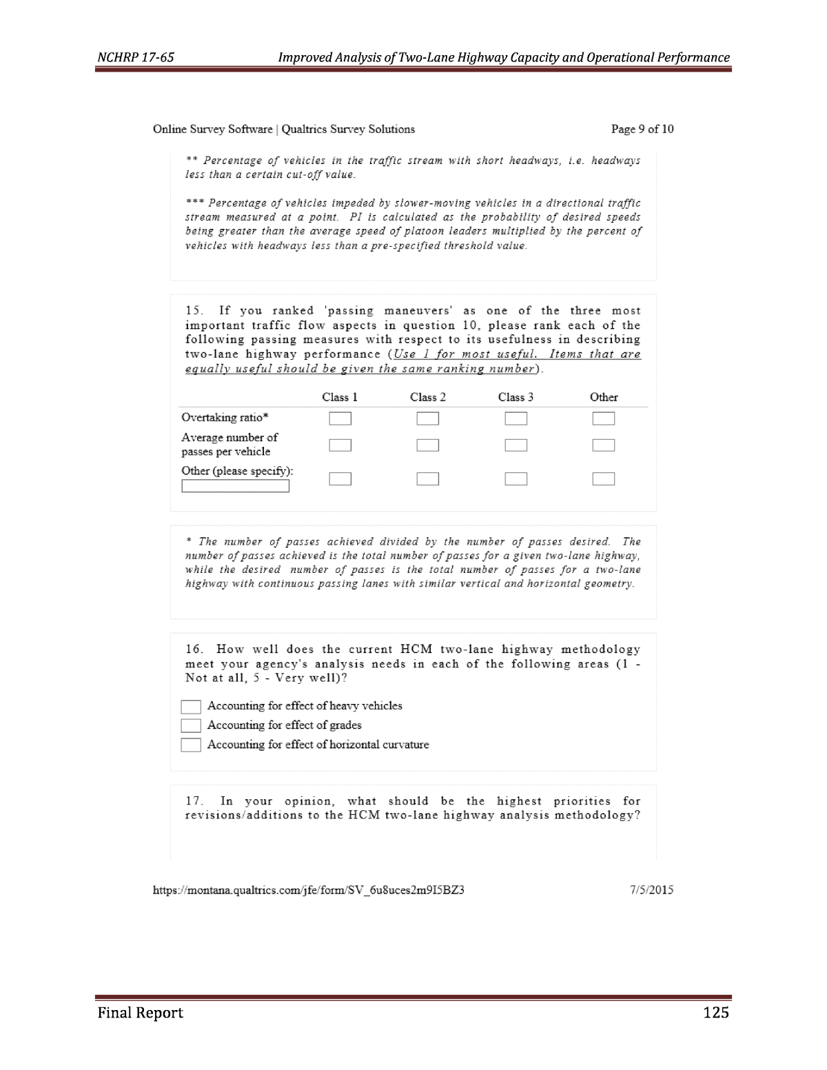
NCHRP 17-65 Improved Analysis of Two-Lane Highway Capacity and Operational Performance Final Report 116 another measure introduced by the South African National Roads Agency and is calculated as the product of percent followers (PF), defined earlier, and traffic density (Van As and Niekerk, 2004). A.1.4. Headway-Related Measures Time headway, which is a microscopic traffic flow characteristic, is another measure used in practical applications as well as in published research. An important measure in this category is PF. Percent impeded (PI) is another measure in this category, which is defined as the product of PF and the probability of desired speeds being greater than the average speed of platoon leaders (Al-Kaisy and Freedman, 2011). A.1.5. Passing-Related Measures Limited passing opportunities are believed to contribute to the formation of platoons and increased delay on two-lane highways. Overtaking ratio and the average number of passes per vehicle are two proposed measures in this category (Luttinen, 2001; Morrall and Werner, 1990; McLean, 1989). The overtaking ratio is estimated by dividing the number of passes achieved by the number of passes desired (Morrall and Werner, 1990). The survey is shown, over the following 10 pages, in Figure A-1.
NCHRP 17-65 Improved Analysis of Two-Lane Highway Capacity and Operational Performance Final Report 117
NCHRP 17-65 Improved Analysis of Two-Lane Highway Capacity and Operational Performance Final Report 118
NCHRP 17-65 Improved Analysis of Two-Lane Highway Capacity and Operational Performance Final Report 119
NCHRP 17-65 Improved Analysis of Two-Lane Highway Capacity and Operational Performance Final Report 120
NCHRP 17-65 Improved Analysis of Two-Lane Highway Capacity and Operational Performance Final Report 121
NCHRP 17-65 Improved Analysis of Two-Lane Highway Capacity and Operational Performance Final Report 122
NCHRP 17-65 Improved Analysis of Two-Lane Highway Capacity and Operational Performance Final Report 123
NCHRP 17-65 Improved Analysis of Two-Lane Highway Capacity and Operational Performance Final Report 124
NCHRP 17-65 Improved Analysis of Two-Lane Highway Capacity and Operational Performance Final Report 125
NCHRP 17-65 Improved Analysis of Two-Lane Highway Capacity and Operational Performance Final Report 126 Figure A-1. Agency Survey on Performance Measures
NCHRP 17-65 Improved Analysis of Two-Lane Highway Capacity and Operational Performance Final Report 127 A.2. Survey Responses A total of 41 responses were received, representing transportation agencies at 25 states and 4 Canadian provinces. The response rate for the U.S. and Canada were 49% and 40%, respectively. There were three states with more than one responseâOregon, California and Texas with 4, 3 and 2 responses, respectively. It should be noted that five state agencies and one Canadian agency submitted the survey without answering any of the questions and therefore, were excluded from the analysis. Figure A-2 identifies the responding U.S. states and Canadian provinces. Figure A-2. Survey participating agencies in the U.S. and Canada (in gray) A.3. Survey Results As previously mentioned, the survey included questions about the agency practice as well as other questions that are more related to respondentsâ perceptions and preferences. A summary of survey results is provided in this section.
NCHRP 17-65 Improved Analysis of Two-Lane Highway Capacity and Operational Performance Final Report 128 A.3.1. Agency Practice Use of Current HCM Methodology When asked about the use of HCM 2010 methodology for two-lane highways, all responding agencies in the U.S. and Canada confirmed the use of the HCM methodology, except one state agency. That agency reported the use of crash analysis and Synchro/Simtraffic software packages for their analysis, and the HCM procedures are used as a supplementary tool if more information is required. However, Synchro/Simtraffic does not have the capability to model two-lane highway operations. Further, the Interactive Highway Safety Design Model (IHSDM) TWOPAS was mentioned as a supplemental analysis tool besides the HCM by another state. Oregon utilizes follower density for analysis of class I and class II highways; however, the HCM is used for analysis of class III highways. Performance measures used for two-lane highway operational analysis Survey participants were asked about the performance measures used by their agency in the operational analysis of two-lane highways. These results are shown in Figure A-3. Figure A-3. Performance measures used in two-lane highway operational analysis ATS and PTSF, followed by PFFS, are used the most for performance analysis on two-lane highways. Only Oregon reported the use of follower density for performance analysis on two-lane highways. Percent followers for vehicles traveling at headways of less than 2 seconds is used by the ministry of Transportation and Infrastructure in British Columbia, Canada. The use of traffic counts, delay, and speed differential for two-lane highway operational analysis was also mentioned by another state agency. Several other performance measures were reported in the survey and they include: annual average daily traffic (AADT), the ratio of AADT to capacity (AADT/c), volume- to-capacity ratio (v/c) and the location and size of available passing areas. Average travel speed (ATS), 83% Percent time spent following (PTSF), 83% Average speed as a percent of free-flow speed (PFFS), 45% Percent followers, 7% Follower density, 3% Other, 21%
NCHRP 17-65 Improved Analysis of Two-Lane Highway Capacity and Operational Performance Final Report 129 Data Collected In Support of Performance Measurement on Two-Lane Highways The survey asked participants about the data collected by their respective agencies that is used in assessing performance on two-lane highways. The results are summarized in Figure A-4. As shown in this figure, almost all highway agencies in the U.S. and Canada use binned vehicle counts as part of their regular data collection programs on two-lane highways. Per vehicle data, which is critical in estimating some performance measures on two-lane highways, is only collected by 17% of the responding agencies. Maine reported the use of speed-delay runs in assessing two-lane highway performance. The Ministry of Transportation and Infrastructure in British Columbia, Canada reported the use of per-vehicle data on two-lane highways on an ad-hoc basis. Figure A-4. Traffic data collected by highway agencies for assessing performance Practitionersâ Perception of Two-Lane Highway Performance Measures Some of the survey questions ask about the participant opinion of the various aspects related to performance measures on two-lane highways. As was mentioned before, there were a total of 35 responses representing 25 states and 4 Canadian provinces. For the analysis of these questions, all responses are considered even if multiple responses came from the same agency, as those responses are more related to individualsâ opinions. A discussion of these questions and their responses is provided below. Characteristics of Good Performance Measures on Two-Lane Highways This survey attempted to gain a better understanding of what constitutes a good performance measure for two-lane highways. Several characteristics of performance measures were identified in this survey and participants were asked to rank these characteristics based on their relative importance for each class of two-lane highways. The characteristic with the highest importance was given a rank of â1â and the rank increases with the decrease in importance. A summary of the participantsâ rankings is presented in Figure A-5 for the three classes of two-lane highways. Speed measurements (binned) , 62.07% Vehicle counts (binned) , 100.00%Heavy vehicle counts (binned) , 86.21% Per-vehicle headway data , 17.24% Per-vehicle speed data , 17.24% Individual vehicle classifications , 41.38% Other , 17.24%
NCHRP 17-65 Improved Analysis of Two-Lane Highway Capacity and Operational Performance Final Report 130 As shown in this figure, the most important characteristic in a two-lane highway performance measure is being sensitive to traffic conditions, as perceived by survey participants. The second characteristic in importance is being sensitive to road conditions. Figure A-5. Average ranking for characteristics of performance measures Road conditions on two-lane highways include such features as horizontal and vertical alignment, lane width and shoulder width. Road user perception of the quality of ride is the third most important characteristic in a performance measure, as ranked by survey participants. The remaining characteristics of performance measures were ranked almost the same with an average ranking of around 3.0. Rankings for different classes of two-lane highways were largely similar, particularly for the three most important characteristics discussed earlier, as clearly shown in Figure A-5. Traffic Flow Aspects and Two-Lane Highway Performance The current survey asked participants to rank several aspects of traffic flow with respect to their usefulness in assessing performance on two-lane highways. Figure A-6 summarizes the responses to this question, with the lowest rank representing the most useful traffic flow aspect, and vice versa. 0.00 0.50 1.00 1.50 2.00 2.50 3.00 3.50 Reflects road user perception Easy to measure in the field Easy to understand / interpret by analysts Sensitive to traffic conditions Sensitive to roadway conditions Compatible with performance measures on other facilities Describes all flow regimes (congested & uncongested) Supports other analyses: including safety, environmental, reliability and economic analyses A ve ra ge R an ki ng Characteristics of a Good Performance Measure Class 1 Class 2 Class 3
NCHRP 17-65 Improved Analysis of Two-Lane Highway Capacity and Operational Performance Final Report 131 Figure A-6. Average ranking score of traffic flow aspects As Figure A-6 depicts, speed was ranked as the most useful aspect of traffic flow in assessing performance on two-lane highways. The rankings for class I and class II highways are almost identical with the most useful traffic flow aspects ranked in the following order: speed, flow, delay, headways, passing maneuvers and density. The corresponding ranking for class III highways resulted in the following order: speed and delay, followed by flow, headways, density and passing maneuvers respectively. The latter ranking is logical given the fact that delay is an important performance measure for interrupted traffic streams and that passing maneuvers may not represent an important aspect of traffic operations in relatively developed areas where major driveways, intersections and auxiliary turning lanes exist. Performance Measures on Two-Lane Highways The survey questionnaire presented the participants with a series of questions asking about the most appropriate two-lane highway performance measures, in relation to those traffic flow aspects discussed in the previous question. Table A-1 presents the average rankings for each performance measure grouped by different traffic flow aspects (a rank of 1.0 represent the best performance measure). 0.00 0.50 1.00 1.50 2.00 2.50 3.00 3.50 Flow Speed Density Platooning / headways Delay Passing maneuvers Av er ag e R an ki ng Traffic Flow Aspect Class 1 Class 2 Class 3
NCHRP 17-65 Improved Analysis of Two-Lane Highway Capacity and Operational Performance Final Report 132 Table A-1. Average Ranking Score for Performance Measures Traffic Flow Aspect Performance Measure Average Ranking Score Class I Class II Class III Flow Volume-to-Capacity (v/c) Ratio 1.56 1.52 1.63 Flow Rate 1.61 1.74 1.77 Follower Flow (FF) 2.14 2.09 2.23 Speed Average Travel Speed (ATS) 1.54 1.52 1.65 Average Travel Speed as a Percent of Free-Flow Speed (PFFS) 2.12 2.20 2.09 Average Travel Speed of Passenger Cars (ATSPC ) 2.44 2.31 2.43 Speed Variance 2.33 2.56 2.58 ATSPC as a Percent of Free-Flow Speed of Passenger Cars (PFFSPC) 2.84 2.92 3.10 Density Traffic Density 1.44 1.56 1.85 Follower Density (FD) 1.38 1.61 1.65 Platooning / Headways Average Platoon Length (# of vehicles) 2.29 2.35 2.53 Percent Time Spent Following (PTSF) 1.44 1.61 1.89 Percent Followers (PF) 2.19 2.31 2.44 Percent Impeded (PI) 2.29 2.41 2.41 Passing Maneuvers Overtaking Ratio 1.15 1.42 1.91 Average Number of Passes per Vehicle 1.83 2.00 2.30 Bold underlined values represent the best average ranking for each class by traffic flow aspect The relative rankings shown in Table A-1 suggest a high level of consistency across the three classes of two-lane highways. Among flow-related performance measures, v/c ratio was ranked first followed by traffic flow and FF, respectively. With regard to speed-related measures, average travel speed was ranked first, followed by average travel speed as a percent of free-flow speed (PFFS), average travel speed of passenger cars (ATSPC), speed variance and ATSPC as a percent of free-flow speed of passenger cars (PFFSPC) respectively. For density-related measures, traffic density is perceived as a better performance measure on class II highways, while follower density (FD) is perceived as a better measure on class I and class III highways. For headway-related performance measures, the HCM measure percent-time-spent-following (PTSF) is perceived the best followed by percent followers (PF), percent impeded and average platoon length respectively. PF is used in the current HCM as a surrogate measure for estimating PTSF using field data. Finally, for measures related to passing maneuvers, overtaking ratio is perceived as a better performance measure compared to the average number of passes per vehicle on a two-lane highway segment.
NCHRP 17-65 Improved Analysis of Two-Lane Highway Capacity and Operational Performance Final Report 133 While Table A-1 is useful in comparing performance measures that belong to the same group/category, it cannot be used to provide objective comparisons across categories. Specifically, the number of measures in each group is different, and therefore, the same average ranking in two different groups could indicate different levels of merit. Limitations of Current HCM Performance Measures Around 73% of the agencies surveyed mentioned they were satisfied with HCM two-lane highway performance measures used by their agencies. Several issues were raised by survey participants, which corresponded to what they perceive as limitations in the current performance measures used on two-lane highways. Some of the comments made in this regard are as follows: ⢠PTSF is difficult to measure in the field. ⢠The level of service based on PTSF is overestimated, especially in summer peak traffic, in that everyone is following someone else. ⢠Even if all vehicles are driving at speeds near speed limit or above, level of service based on PTSF would be F. ⢠The PTSF does not recognize or rate context of a project segment within an entire corridor between control cities. ⢠For class 1 highways with high volume, the PTSF dictates the LOS results; however the HCM suggests using both the ATS and the PTSF for class 1 highways. Proposed Changes to Use of Performance Measures on Two-Lane Highways As was mentioned earlier, there are some limitations related to the current HCM methodology for operational analysis of two-lane highways as reported in several studies in the literature (Al-Kaisy and Freedman, 2011; Al-Kaisy and Freedman, 2010; Al-Kaisy, A., and S. Karjala, 2008; Brilon, W., and F. Weiser, 2006; Luttinen, 2001). Survey participants were asked to state their priorities for revisions/additions to the HCM two-lane highway analysis methodology. The following is a summary of their feedback as related to the use of performance measures on two-lane highways. A few characteristics were mentioned by survey participants as being important for a good performance measure on two-lane highways. One respondent mentioned that the performance measure should be able to describe the whole corridor between control cities/towns. Overall travel time was mentioned as an example of such performance measures. Other respondents suggested the use of other measures not included in the survey such as travel time reliability. One survey respondent mentioned that the travelersâ experience along the whole corridor should be considered by any proposed new measure. Replacing PTSF and ATS with more follower (headway) based measures like follower density was recommended by another survey respondent. Other criteria that were mentioned by survey participants as being important for performance measures are consistency between facilities in different area types (urban, suburban, rural) and the ease with which the measures can be explained to the public. A.4. Summary of Findings In an attempt to better understand the transportation agencyâs perspective with regard to what constitutes a good performance measure for two-lane highways, a questionnaire survey was sent to all state DOTs in the U.S. and the provincial ministries of transport in Canada. The survey also
NCHRP 17-65 Improved Analysis of Two-Lane Highway Capacity and Operational Performance Final Report 134 included a few questions about the agency experience with the use of the HCM and proposed changes and revisions to the current analytical procedures. A total of 35 usable responses were received, representing transportation agencies at 25 states and 4 Canadian provinces. The most important findings of the survey on the use of two-lane highway performance measures are summarized below: ⢠Almost all highway agencies reported the use of the current HCM performance measures on two-lane highways, i.e., average travel speed, percent-time-spent-following, and percent of free flow speed. Among other non-HCM measures used by some agencies were follower density, percent follower for vehicles traveling at headways of less than 2 seconds, traffic flow, delay, v/c ratio and AADT/c ratio. ⢠While almost all highway agencies in the U.S. and Canada use binned vehicle counts as part of their regular data collection programs on two-lane highways, per vehicle data, which is critical in estimating some performance measures on two-lane highways, is only collected by 17% of the responding agencies. This restricts the ability of those agencies in using many performance measures included in this survey, which require the more detailed per vehicle data. ⢠The top three criteria that were ranked as being most important characteristics for two- lane highway performance measures are: sensitivity to traffic conditions, sensitivity to road conditions, and relevance to road user perception, respectively. ⢠Among traffic flow aspects that are most relevant to two-lane highway operations, speed followed by flow were ranked as the most important aspects for all two-lane highway classes. ⢠With regard to the merit of using individual performance measures within each traffic flow aspect category, the best measures were found to be v/c ratio, average travel speed, PTSF, and overtaking ratio for all two-lane highway classes in the flow, speed, headways and passing maneuvers categories respectively. For the density flow aspect, follower density was found superior on class I and class III while density was found superior on class II two-lane highways. Percent followers, used by the current HCM as a surrogate measure for PTSF, was associated with much lower average ranking compared with PTSF for all highway classes. The responses to the practice survey included some of the limitations of the current HCM performance measures from the agenciesâ perspective, as well as some valuable suggestions and feedback on two-lane highway performance measures that were discussed in the paper. The results from the agency survey revealed that a wide range of performance measures are used by agencies. The results suggest that the top three criteria for good performance measures on two-lane highways are: sensitivity to traffic conditions, sensitivity to road conditions, and relevance to road user perception. Further, agencies identified average travel speed as the most relevant traffic flow aspect to two-lane highway operations. Other performance measures that were found meritorious were volume-to-capacity ratio and flow rate, for class I and class II highways, respectively, versus average travel speed, volume-to-capacity ratio, and percent-time- spent-following for class III highways.
NCHRP 17-65 Improved Analysis of Two-Lane Highway Capacity and Operational Performance Final Report 135 B. Service Measure Evaluation B.1. Introduction Performance measures are essential for assessing the quality of service, which describes how well a transportation facility or service operates from a travelerâs perspective (TRB, 2010). From a highway agencyâs perspective, performance measures are essential in determining the need for operational improvements on two lane highways (e.g., passing lanes) or the need to upgrade to a multi-lane highway. Ideally, performance measures used for traffic operations and capacity analysis should (Luttinen et al., 2005): 1. Reflect the perception of road users on the quality of traffic flow. 2. Be easy to measure, estimate, and interpret. 3. Correlate to traffic and roadway conditions in a meaningful way. 4. Be compatible with the performance measures of other facilities. 5. Describe both uncongested and congested conditions. 6. Be useful in analyses concerning traffic safety, reliability, transport economics, and environmental impacts. The six criteria above consider the common operational objectives of most highway agencies, namely: mobility (criterion 1), productivity (criteria 2, 3 and 5), safety (criterion 6), reliability (criterion 6) and low environmental impacts (criterion 6). This chapter discusses current performance measures in the Highway Capacity Manual (HCM), other performance measures proposed in the literature, an empirical evaluation of potential performance measures, and finally the selection of performance/service measures for the new two-lane highway analysis methodology. B.2. Highway Capacity Manual Performance Measures The current HCM (TRB, 2016) classifies two-lane highways into three different classes based on the degree to which they serve mobility and the adjacent land use character (e.g., rural versus developed areas). These classes are: a. Class I two-lane highways: Highways where motorists expect to travel at relatively high speeds and they include major intercity routes, daily commuter routes, and major links in state or national highway network. b. Class II two-lane highways: Highways where motorists do not necessarily expect to travel at high speeds and they include access routes to class I facilities, some scenic and recreational routes, and routes passing through rugged terrain. c. Class III two-lane highways: These primarily include highways serving moderately developed areas. They may be portions of class I and class II highways that pass through small towns or developed recreational areas. Traffic stream characteristics on each of these highway classes are different and as such different performance measures are proposed. A total of three performance measures are used in the current HCM analysis methodology for the assessment of level of service (hereafter referred to as service
NCHRP 17-65 Improved Analysis of Two-Lane Highway Capacity and Operational Performance Final Report 136 measures), namely: percent time spent following (PTSF), average travel speed (ATS), and percent of free flow speed (PFFS). PTSF is defined as the average percent of total travel time that vehicles must travel in platoons behind slower vehicles due to the inability to pass (TRB, 2010). PTSF represents the freedom to maneuver and the comfort and convenience of travel and is used on class I and class II two-lane highways (TRB, 2010). While this performance indicator may relate well to the quality of service on two-lane highways, it is impractical to measure in the field. Therefore, the HCM recommends the use of a surrogate measure, referred to in this study as percent followers (PF), for field estimation of PTSF. PF is defined as the percentage of vehicles in the traffic stream with time headways smaller than 3 seconds. ATS on the other hand reflects mobility and is defined as the highway segment length divided by the average travel time taken by vehicles to traverse it during a designated time interval (TRB, 2010). ATS is considered for estimating performance on class I two-lane highways only. Finally, PFFS represents the ability of vehicles to travel at or near the posted speed limit and is measured as the ratio of ATS to free flow speed (FFS) multiplied by 100 (TRB, 2010). PFFS is used as the service measure only for class III two-lane highways. Limitations in the HCM methodology for measuring performance on two-lane highways have been reported in several studies and some of those limitations are concerned with the appropriateness of the service measures used (Al-Kaisy and Freedman, 2011; Al-Kaisy and Freedman, 2010; Al-Kaisy and Karjala, 2008; Brilon and Weiser, 2006; Luttinen, 2001). Specifically, the PTSF is difficult to measure in the field and does not readily describe the extent of congestion on the facility, which is important for operational analysis and highway improvement decisions. Average travel speed, on the other hand, is easy to measure in the field; however, it is not very sensitive to traffic level on the highway. Since the analysis section of a two- lane highway facility is usually several miles long, there could be many changing conditions, such as posted speed limit and roadway alignment that affect ATS, yet it is not related to varying traffic conditions. This can make ATS somewhat meaningless for determining how the highway is operating (Al-Kaisy and Freedman, 2011). The PFFS is meant to account for the limitations of ATS as it measures the speed reduction due to increased traffic volume and/or platooning, which makes it possible to compare the current conditions to the ideal conditions (Al-Kaisy and Freedman, 2011). One of the limitations of PFFS is that it is largely unaffected by the addition of a passing lane, which indicates that it is not particularly helpful in capturing the delay caused by platooning (Al-Kaisy and Freedman, 2010). B.3. Alternative Performance Measures A number of alternative performance and/or service measures for two-lane highways have been suggested in the literature. Most of the studies that proposed new performance measures were driven by the obvious limitations of the HCM procedures, including those of the performance measures used. As discussed previously, PTSF is difficult to measure in the field, is not compatible with the service measures of other facilities, does not describe the extent of congestion, and is not very useful in other analyses. PTSF is also a poor performance measure for indicating if improvements should be made to a highway that has low volumes with a high percentage of heavy vehicles and few passing opportunities. ATS, on the other hand, is not very informative about the efficiency of the highway. Since the analysis section of a two-lane highway facility is usually
NCHRP 17-65 Improved Analysis of Two-Lane Highway Capacity and Operational Performance Final Report 137 several miles long, there could be many changing conditions, such as posted speed limit and roadway alignment that affect ATS, yet it is not related to varying traffic conditions. In this section, a review of alternative performance measures that have been proposed in the literature or reported as part of current practice is presented. The review does not include the two measures currently used by the HCM procedures, PTSF and ATS, as these two measures were discussed previously. In this document, the use of the term âperformance measureâ is intended to refer to the performance measure, or measures, that would be used to base the classification of LOS upon; that is, the âservice measureâ. In this section, performance measures are classified and presented in the following common categories: 1. Speed-related measures 2. Flow-related measures 3. Density-related measures 4. Measures related to passing maneuvers 5. Combination measures B.3.1. Speed-Related Measures The vast majority of two-lane highways can be thought of as âuninterrupted flow facilitiesâ, thus enjoying relatively higher travel speeds. This is particularly true for class I highways, which represent important arterials and major collectors in rural areas. On these highways, ATS has long been used by the HCM as a performance measure with the premise that average speed is affected by traffic level and, thus, the amount of platooning due to limited passing opportunities. However, two-lane highways involve most of highway classifications, have a wide range of geometric standards, and consequently, a wide range of operating speeds. Therefore, using average speed alone may not provide enough information about the level of traffic performance (in the absence of a reference point) to make performance comparison across sites practical. In their investigation of proposed performance measures, Al-Kaisy and Karjala (2008) examined three speed-related measures: ⢠Average travel speed of passenger cars (ATSPC) ⢠ATS as a percent of free-flow speed (ATS/FFS) ⢠ATSPC as a percent of free-flow speed of passenger cars (ATSPC/FFSPC) The researchers argued that average travel speed of passenger cars may more accurately describe speed reduction due to traffic, since passenger car speeds are more affected by high traffic volumes than heavy vehicle speeds. Further, using ATS as a percentage of free-flow speed was viewed as a good indicator of the amount of speed reduction due to traffic and the amount of vehicular interaction in the traffic stream. However, evaluations using field data showed that the speed measures did not exhibit good correlations with platooning variables as compared to other performance measures investigated in the study. Luttinen (2001a) reported on a study by Kiljunen and Summala in 1996 which proposed the use of ATS/FFS as a performance measure on Finnish two-lane highways.
NCHRP 17-65 Improved Analysis of Two-Lane Highway Capacity and Operational Performance Final Report 138 In their article on the German experience, Brilon and Weiser (2006) reported the use of average speed of passenger cars over a longer stretch of highway, averaged over both directions, as a major performance measure on two-lane highways. Truck speeds are not very sensitive to increases in traffic volume, but traffic volume is the main factor affecting the ATS of passenger cars (Brilon and Weiser, 2006). In his study on PTSF in Finland, Luttinen (2001) reported on an old study by O.K. Normann, who suggested the use of speed differences between successive vehicles on two-lane highways among other proposed performance measures. A study by Washburn et al. (2002) proposed a third class for two-lane highways and the service measure of ATS/FFS for this class. This proposed third class and corresponding service measure is intended to apply to two-lane highways that are considered scenic in nature (e.g., along a coastline) and/or serve well-developed areas. For these situations, it was determined that drivers do not have much expectation for being able to pass other vehicles and that their main desire is to be able travel at a speed close to the free-flow speed. A study by Yu and Washburn (2009) and Li and Washburn (2014) proposed the percent delay service measure for two-lane highway facilities (i.e., a combination of two-lane highway segments and intersections). This service measure is based on the difference between free-flow travel time and actual travel time. The use of a speed-based measure allows the service measure to be applied to both two-lane highway segments and intersections, which individually use delay as the service measure. B.3.2. Flow-Related Measures Several flow-related measures have been used in practice or proposed in the literature for measuring performance on two-lane highways. This is somewhat expected, given that traffic flow level is largely associated with platooning and delay and, consequently, with usersâ perception of the quality of service. The v/c ratio, or degree of capacity utilization, has been used as the main performance measure on two-lane highways in Denmark, China and Japan (Vejdirektoratet, 2010; Rong et al., 2011; Nakamura & Oguchi, 2006). It is important to note that the two-lane expressways in Japan are different from the conventional two-lane highways in the U.S. and most other countries in that they have limited access (no at-grade intersections) and a median barrier present in all sections (Catbagan and Nakamura, 2006). Further, the v/c ratio has been used as an additional performance measure in Sweden (Trafikverket, 2014). Another measure that has been used extensively both in practical applications as well as in published research is time headway, a major traffic flow microscopic characteristic. For various practical reasons, time headway has been used solely for identifying platoons using empirical traffic data and field measurements. One important reason for using time headway is that this measure can readily be extracted from the output of conventional traffic recorders, which have the ability to provide raw data (i.e., timestamp records for individual vehicle arrivals). The second equally important reason is the fact that time headway is a good indicator of the interaction between successive vehicles in the traffic stream and, thus, in determining the status of a vehicle being in a following mode (i.e., being part of a vehicular platoon).
NCHRP 17-65 Improved Analysis of Two-Lane Highway Capacity and Operational Performance Final Report 139 The most commonly used headway-based service measure is percent followers (PF). PF is used by the HCM to estimate PTSF with field data. It is defined as the percentage of vehicles in the traffic stream with headways of less than three seconds (TRB, 2000, 2010). A few recent studies have examined PF along with other proposed performance measures to evaluate their suitability for use on two-lane highways (Al-Kaisy and Karjala, 2008; Catbagan and Nakamura, 2006; Hashim and Abdel-Wahed, 2011; Van As, 2003; ODOT, 2014). Another headway-based measure that was reported in the literature is follower flow, which was investigated by the South African National Roads Agency (Van As, 2003). It is defined as the hourly rate of vehicles in following mode that pass a point along a two-lane highway. This measure can easily be estimated as the product of PF and the flow rate. Follower flow was investigated among several other performance measures in the development of the current South African two-lane highway methodology. While this performance measure was found superior to most other performance measures investigated by this study, it was outperformed by follower density that was eventually adopted for use as a service measure in the current South African two- lane highway methodology. B.3.3. Density-Related Measures In their study, Brilon and Weiser (2006) reported that the then current German Capacity Handbook (HBS, 2001) utilized density as the primary service measure for two-lane highways. Density is calculated as the ratio of traffic volume and the ATS of just passenger cars (i.e., ATSpc). The rationale for using density as a performance measure on two-lane highways in Germany is that efficiency is given preference over user experience (perception) of the quality of service (Brilon and Weiser, 2006). Further, this performance measure is compatible with other facility types, mainly freeways and multi-lane highways, when those highway types are analyzed as part of a larger system. B.3.4. Measures Related to Passing Maneuvers The platooning phenomenon on two-lane highways and the associated delay are directly related to passing opportunities and the ability of platoon vehicles to pass slower vehicles and improve their speeds. As such, a few performance measures were proposed for assessing performance on two- lane highways that are related to passing maneuvers. A study by Morrall and Werner (1990) proposed the use of overtaking ratio as a supplementary indicator of the level of service on two-lane highways. This measure is obtained by dividing the number of passes achieved by the number of passes desired. According to the study, the number of passes achieved is the total number of observed passes for a given two-lane highway, while the number of passes desired is the total number of passes for a two-lane highway with continuous passing lanes with similar vertical and horizontal geometry. Overtaking ratio, along with the average number of passes per vehicle, were also proposed by O.K. Norman, as reported by McLean (1989), and Luttinen (2001).
NCHRP 17-65 Improved Analysis of Two-Lane Highway Capacity and Operational Performance Final Report 140 B.3.5. Combination Measures A couple of measures proposed in the literature are associated with more than one traffic stream parameter, and as such, they are discussed independently from the previous measures. The merit of using compound measures is the fact that those measures usually combine the advantages of more than one indicator of traffic performance on two-lane highways (e.g., amount of platooning and traffic level). One important combination measure is follower density, which was originally adopted by the South African National Roads Agency about ten years ago (Van As, 2003; Van As and Niekerk, 2004) and was later investigated in other studies (Catbagan and Nakamura, 2006; Al-Kaisy and Karjala, 2008; Hashim and Abdel-Wahed, 2011; Moreno et al., 2014). Follower density is defined as the product of PF and traffic density; therefore, this measure is derived using two important flow characteristics: traffic flow and density. Again, PF is estimated using time headway, which is a microscopic flow characteristic. Another combination measure that was proposed in the literature is percent impeded. This measure was originally proposed by Al-Kaisy and Freedman (2011) and was later investigated by Hashim and Abdel-Wahed (2011), Ghosh et al. (2013), and Moreno et al. (2014). PI is defined as the product of PF and the probability of desired speeds being greater than the average speed of platoon leaders. Therefore, this measure is derived using flow and speed characteristics. B.4. Preliminary Assessment of Proposed Performance Measures In this section, an initial qualitative assessment of the proposed alternative performance measures is presented. The HCM performance measures will also be included in this assessment to help in understanding the merits of the proposed alternative measures. As discussed earlier in this report, it is desired for prospective performance measures on two-lane highways to meet the following criteria. 1. Performance measure should reflect the perception of road users on the quality of traffic flow. ⢠It is a common understanding that platooning and lack of passing opportunities (and its associated delay) primarily affect the motoristsâ perception of the quality of service on two-lane highways. 2. Performance measure should be easy to measure and estimate using field data. ⢠Specifically, it is expected that the performance indicator of choice can be measured in the field using conventional data collection methods used by highway agencies and the professional community. 3. Measure should correlate to traffic and roadway conditions in a meaningful way. ⢠On two-lane highways, the prospective performance measure should closely correlate to the platooning phenomenon (and passing opportunities) as well as to traffic level in a logical and meaningful way. 4. It is recommended that the prospective measure be compatible with performance measures used on other facilities.
NCHRP 17-65 Improved Analysis of Two-Lane Highway Capacity and Operational Performance Final Report 141 ⢠This criterion may be hard to satisfy as it is expected that different aspects of traffic operations are perceived as most important by drivers on different highway facilities. For example, while platooning on two-lane highways is a major determinant of the quality of operation, it is not a major factor in determining the quality of operations on other facilities. 5. Performance measure should be able to describe both uncongested and congested conditions. ⢠While this requirement is applicable to all highway facilities per the definition of the LOS scheme, it has been perceived to have less significance on two-lane highways, since these facilities are rarely congested and are usually upgraded to four lanes when they do become congested. 6. Measure should be useful in analyses concerning traffic safety, transport economics, and environmental impacts. ⢠Increasingly, the capacity analysis procedures have been used in supporting the aforementioned analyses. To be of use in safety analyses, the prospective measure should correlate well to traffic exposure. On the other hand, for economic and environmental impact analyses, the prospective measure should be useful in estimating delay and its associated fuel consumption and tailpipe emissions. Table B-1 summarizes all of the performance measures discussed in this report and the degree to which each measure satisfies the six criteria discussed above. In this subjective assessment, each performance measure is evaluated against the six criteria independently (i.e., assessed assuming itâs used solely for measuring performance on two-lane highways). At a glance, it can be clearly seen that no single measure largely satisfied all evaluation criteria and that each measure satisfied some criteria to a higher degree but scored low on other criteria. Therefore, identifying a single performance measure that satisfactorily meets all of the above criteria may not be realistic.
NCHRP 17-65 Improved Analysis of Two-Lane Highway Capacity and Operational Performance Final Report 142 Table B-1. Preliminary assessment matrix of performance measures on two-lane highways Performance Measure Type a (1) Road User Perception (2) Easy to Measure (3) Sensitive to Road Conditions (4) Compatible with Other Facilities (5) Describes All Flow Regimes (6) Support Other Analyses Safety Economic Environmental Reliability HCM â PTSFb FR XXXc X X X Xd X X X X HCM â ATS SR X XXX X XX Xd XX XX XX X HCM â (ATS/FFS) SR XX XXX XX X XXd X XXX XXX X Average travel speed of passenger cars (ATSPC) SR X XXX X XX XXX X XX XX X ATSPC as a percent of free-flow speed of passenger cars (ATSPC/FFSPC) SR XX XXX XX X XXX X XXX XXX X Speed Variance SR X XXX X X X XX X X X Demand-to-capacity (d/c) ratio FR XX XXX X X XXX XX XX XX XX Percent followers (PF) FR XX XX XX X X X X X X Follower flow FR X XX XX X X XX X X X Traffic density DR XX XXX XX XXX XXX XXX X X XX Overtaking ratio PASS X X XX X X X X X X Average number of passes per vehicle PASS X X XX X X XX X X X Follower density (FD) COMB XX XX XX XX X XX X X X Percent impeded (PI) COMB XX XX XXX X X XX X X X a â SR = speed-related, FR = flow-related, DR = density-related, PASS = passing maneuvers, COMB = combination b â PTSF is estimated using flow rates in the analytical methodology and using percent followers (PF) as a surrogate measure for field estimation. c â X = hardly meeting criterion, XX = fairly meeting criterion, XXX = largely meeting criterion d â Level of service F is not defined for any of the three HCM 2010 performance measures
NCHRP 17-65 Improved Analysis of Two-Lane Highway Capacity and Operational Performance Final Report 143 B.5. Empirical Analysis of Field Data This section presents an empirical investigation into several two-lane highway performance measures that have been used in practice or proposed in the literature for operational analysis on two lane highways. Those performance measures included average travel speed, average travel speed to free flow speed, percent followers, follower flow, follower density, percent impeded, impeded flow and impeded density. Field data from 16 study sites, four in Montana, four in Idaho, four in Oregon and four in North Carolina were used in this study. The level of association between performance measures and some of the most important traffic variables were examined in this study. The traffic variables investigated in this study included combined flow in both direction of travel, traffic split, percentage of heavy vehicles and speed variance. B.5.1. Study Design In order to assess the suitability of performance measures, the association between several performance measures and traffic variables were investigated in this research. Traffic variables investigated consisted of combined flow in both directions of travel, heavy vehicle percentage (% HV), traffic split (proportion of traffic in travel direction), speed variance and percent no passing zone. Performance measures used in this investigation include: ⢠Average Travel Speed (ATS): Average speed of all vehicles traveling in the direction of analysis. ⢠Average Travel Speed to Free Flow Speed (ATS/FFS): The ratio between the average travel speed of all vehicles to free-flow speed. In this study, the average speed of vehicles with headway more than 8 seconds was used to establish the free-flow speed. ⢠Percent Followers (PF): Percentage of vehicles with headways less than 3 seconds (used by HCM to estimate PTSF using field data). ⢠Follower Density (FD): The number of vehicles in following mode per mile per lane in one direction of travel. This measure is calculated as the traffic density (in one direction) multiplied by percent followers (PF). ⢠Follower Flow (FF): The hourly rate of vehicles in following mode that passes a point along a two-lane highway in the same direction. This measure is calculated as the flow rate multiplied by percent followers (PF). ⢠Percent Impeded (PI): Percentage of vehicles impeded by slower-moving vehicles in a directional traffic stream measured at a point. PI is calculated as the probability of desired speeds being greater than the average speed of platoon leaders multiplied by the percent of vehicles with headways less than a pre-specified threshold value. A threshold value of 3 seconds was used in this study (same as PF). For finding the distribution of desired speeds, vehicles with headway more than 8 seconds were used. Platoon leaders were used as a representative sample of slow moving vehicles. ⢠Impeded Flow (IF): The hourly rate of vehicles being impeded by slow vehicles, i.e., platoon leaders. It is calculated as the product of PI and the hourly rate of traffic flow. ⢠Impeded Density (ID): Number of vehicles impeded per mile per lane in one direction of travel. It is calculated as the product of PI and traffic density. Traffic variables investigated in this study include:
NCHRP 17-65 Improved Analysis of Two-Lane Highway Capacity and Operational Performance Final Report 144 ⢠Combined flow (veh/h): The hourly flow rate in both directions of travel. ⢠Traffic split: The proportion of hourly flow rate in the direction of analysis to combined flow. ⢠Percent heavy vehicles (%HV): The percentage of heavy vehicles in the direction of analysis. ⢠Speed variance: The square of standard deviation of all vehicle speeds measured at a specific location in direction of analysis. ⢠Percent no passing: It shows the percentage of the road in which passing is not allowed. This percentage was found for 3 miles upstream and downstream of the location of traffic counter. It is important to note that while speed variance was reported as one of the proposed performance measures on two-lane highways, it is treated as one of the traffic variables in this analysis. B.5.2. Study Sites Sixteen study sites in the states of Montana, Idaho, Oregon and North Carolina were used in this study (four sites in each state). Traffic volumes, area setting, terrain and number of access points were among the considerations for selecting the sites. All sites are located in rural areas. A brief description of the sites is provided below. 1. ATR 43, Highway US 191 near Big Sky, Montana. This site is located about 1.5 mi north of junction of MT-64 and US 191. Data from Automatic Traffic Recorder (ATR) number A-043 was used for this site. The annual average daily traffic (AADT) at this site is 4,776 vehicles per day in 2014. This site is located in a mountainous area. This site is a principal arterial which is considered as a class 1 highway for the purpose of this study. 2. WIM 132, Highway MT-200 near Greenough, Montana. This site is located about 6 miles north of Greenough. Data from WIM (Weigh in Motion) station A-132 was used for this site. The annual average daily traffic (AADT) at this site is 2,831 vehicles per day in 2014. This site is a principal arterial which is considered as a class 1 highway for the purpose of this study. 3. ATR 28, Interstate 15 Frontage road near Great Falls, Montana. This site is located about 7 mi west of Great Falls and about 4.2 miles east of Vaughn. Data from ATR (Automatic Traffic Recorder) station A-028 was used for this site. The annual average daily traffic (AADT) at this site is 2,939 vehicles per day in 2014. This site is a major collector which is considered as a class 2 highway for the purpose of this study. 4. ATR 73, Highway MT-35 south of Flathead Lake, Montana. This site is located about 2.8 mi east of the junction of US 93 and MT-35. Data from WIM station A-73 was used for this site. The annual average daily traffic (AADT) at this site is 3,562 vehicles per day in 2014. This site is a minor arterial which is located in a relatively developed recreational area and as such is considered as a class 3 highway for the purpose of this study. 5. ATR 47, Highway U.S. 2 near Priest River, Idaho. This site is located about 2.6 mi east of Idaho-Washington border line, on the highway segment that connects Laclede, Idaho to Priest River, Idaho. Data from ATR station A-047 was used for this site. The annual average daily traffic (AADT) at this site is 6,799 vehicles per day in 2014. This site is a principal arterial and is considered as a class 1 highway for the purpose of this study.
NCHRP 17-65 Improved Analysis of Two-Lane Highway Capacity and Operational Performance Final Report 145 6. ATR 44, Highway U.S. 95 near Weiser, Idaho. This site is located about 3.8 mi south of Main Street of Weiser, on the highway segment that connects Wood, Idaho to Weiser, Idaho. Data from ATR station A-044 was used for this site. The annual average daily traffic (AADT) at this site is 5,206 vehicles per day in 2014. This site is a principal arterial and is considered as a class 1 highway for the purpose of this study. 7. ATR 147, SH 57 road near Priest River, Idaho. This site is located about 8.4 mi north of Priest River, Idaho. Data from ATR station A-147 was used for this site. The annual average daily traffic (AADT) at this site is 1,582 vehicles per day in 2014. This site is a major collector and is considered as a class 2 highway for the purpose of this study. 8. ATR 126, Highway U.S. 95 near Moscow, Idaho. This site is located about 0.4 mi north of the junction of Brent Dr. street and U.S. 95. Data from ATR station A-126 was used for this site. The annual average daily traffic (AADT) at this site is 6,391 vehicles per day in 2014. This site is a principal arterial located in a relatively developed area and is therefore considered as a class 3 highway for the purpose of this study. 9. Site 1-NC, Highway U.S. 17 near Maysville, North Carolina. This site is located about 2.6 mi north of Maysville. The annual average daily traffic (AADT) at this site is 9,600 vehicles per day in 2014. This site is a major collector and is considered as a class 1 highway for the purpose of this study. 10. Site 3-NC, Highway U.S. 64 near Manns Harbor, North Carolina. This site is located about 2.5 mi west of Manns Harbor. The annual average daily traffic (AADT) at this site is 3,300 vehicles per day in 2014. This site is a major collector and is considered as a class 1 highway for the purpose of this study. 11. Site 4-NC, Highway U.S. 43 near New Bern, North Carolina. This site is located about 8.2 mi north of New Bern. The annual average daily traffic (AADT) at this site is 2,700 vehicles per day in 2014. This site is a major collector and is considered as a class 1 highway for the purpose of this study. 12. Site 7-NC, Highway U.S. 43 near Vanceboro, North Carolina. This site is located about 3 mi south of Vanceboro. The annual average daily traffic (AADT) at this site is 7,700 vehicles per day in 2014. This site is a major collector and is considered as a class 3 highway for the purpose of this study. 13. Site 2-OR, Highway U.S. 97 near Chiloquin, Oregon. This site is located about 19.5 mi north of Vanceboro. The annual average daily traffic (AADT) at this site is 3,900 vehicles per day in 2014. This site is a major collector and is considered as a class 3 highway for the purpose of this study. 14. Site 11-OR, Highway U.S. 126 near Cloverdale, Oregon. This site is located about 2.5 mi east of Cloverdale. The annual average daily traffic (AADT) at this site is 5,000 vehicles per day in 2014. This site is a major collector and is considered as a class 3 highway for the purpose of this study. 15. Site 13-OR, Highway U.S. 97 near Grass Valley, Oregon. This site is located about 4.9 mi north of Grass Valley. The annual average daily traffic (AADT) at this site is 2,700 vehicles per day in 2014. This site is a major collector and is considered as a class 3 highway for the purpose of this study.
NCHRP 17-65 Improved Analysis of Two-Lane Highway Capacity and Operational Performance Final Report 146 16. Site 17-OR, Highway U.S. 26 near Warm Springs, Oregon. This site is located about 15.8 mi north of Warm Springs. The annual average daily traffic (AADT) at this site is 4,900 vehicles per day in 2014. This site is a major collector and is considered as a class 3 highway for the purpose of this study. According to the 2010 HCM, study sites 1,2,5,6,9,10,11,13,14 and 16 can be classified as class I, sites 3 and 7 are class II and sites 4,8 and 12 are class III. Data for the sites were provided by Montana Department of Transportation, Idaho Transportation Department, Oregon Department of Transportation and North Carolina Department of Transportation. Per vehicle data including arrival time, spot speed, and vehicle classification was obtained from automatic traffic recorder output. A description of the data collected at the 16 study sites is provided in Table B-2.
NCHRP 17-65 Improved Analysis of Two-Lane Highway Capacity and Operational Performance Final Report 147 Table B-2. Description of Field Data at Study Sites Site name Dates Class Duration of data collection (hours) Total vehicle count (veh) Speed Limit (mi/h) Direction of analysis Percent No- Passing Zones ATR 43- MT July 20, 2014- July 26, 2014 I 168 23,676 60 South-bound 93 ATR 132- MT July 9, 2014- July 24, 2014 I 384 31,653 70, 60 (trucks) West-bound 56 ATR 28 - MT July 16, 2015 - July 30, 2015 II 360 24,311 70, 60 (trucks) North-bound 40 ATR 73 - MT July 16, 2015 - July 30, 2015 III 360 47,052 60 North-bound 66 ATR 47-ID June 16, 2015 - June 30, 2015 I 360 62,643 60 West-bound 33 ATR 44-ID June 15, 2015 - June 30, 2015 I 384 49,737 65 North-bound 13 ATR 147- ID September 12,2015- September 20,2015 II 216 8,727 50 North-bound 86 ATR 126- ID September 12,2015- September 20,2015 III 216 33,300 45 South-bound 30 Site 1-NC June 8, 2015-June 16, 2015 I 185 91,790 55 South-bound 37 Site 3-NC June 15, 2015-June 23, 2015 I 172 50,334 55 East-bound 3 Site 4-NC June 9, 2015-June 17, 2015 I 188 93,700 55 North-bound 68 Site 7-NC June 8, 2015-June 16, 2015 III 171 88,082 55 North-bound 30 Site 2-OR July 9, 2015-July 12 2015 I 48 21,932 55 South-bound 17 Site 11-OR May 28,2015- May 31,2015 I 48 19,657 55 East-bound 50 Site 13-OR June 4, 2015-June 7, 2015 I 48 12,596 55 South-bound 30 Site 17-OR June 11 2015-June 14, 2015 I 48 26,757 55 South-bound 55 Study sites are shown in Figure B-1, Figure B-2, Figure B-3 and Figure B-4.
NCHRP 17-65 Improved Analysis of Two-Lane Highway Capacity and Operational Performance Final Report 148 ATR 28 ATR 43 ATR 73 ATR 132 Figure B-1. Montana data collection sites ATR 47 ATR 147 ATR 44 ATR 126 Figure B-2. Idaho data collection sites
NCHRP 17-65 Improved Analysis of Two-Lane Highway Capacity and Operational Performance Final Report 149 Site 17 Site 13 Site 2 Site 11 Figure B-3. Oregon data collection sites Site 1 Site 7 Site 4 Site 3 Figure B-4. North Carolina data collection sites
NCHRP 17-65 Improved Analysis of Two-Lane Highway Capacity and Operational Performance Final Report 150 B.5.3. Research Underlying Hypotheses In this section, the major hypotheses underlying the relationship between performance measures and traffic variables are discussed. The hypothesized behavior of performance measures in response to changes in traffic variables is discussed below. ⢠Combined flow: This is the combined flow in the two directions of travel expressed as an hourly flow rate. As combined flow increases, ATS and ATS/FFS are expected to decrease. On the other hand, all other performance measures (PF, FD, FF, PI, ID, and IF) are expected to increase. ⢠Traffic split: This is the proportion of traffic flow in the analysis direction. The hypotheses here are similar to those of combined flow. For a given total traffic level, as traffic split increases, ATS and ATS/FFS are expected to decrease while all other performance measures (PF, FD, FF, PI, ID, and IF) are expected to increase. ⢠Percent heavy vehicles: Heavy vehicles are generally associated with lower performance and thus lower speeds compared to passenger cars. As heavy vehicle percentage increases, ATS and ATS/FFS are expected to decrease while all other performance measures are expected to increase. ⢠Speed variance: Similar to percent heavy vehicles, this variable is not generally perceived as being related to traffic level, however, it may well be associated with the level of platooning in the traffic stream. The relationship between speed variance and performance measures may not be as straightforward as with the other three traffic variables. On one hand, high-speed variance could mean faster formation of platoons due to faster vehicles quickly catching up with slower vehicles forming platoons (a.k.a. bunches, groupings, etc.). On the other hand, a traffic stream consisting of a high percentage of platooned vehicles may exhibit more uniformity in speeds due to following vehicles roughly traveling at speeds of platoon leaders (thus smaller speed variance). Therefore the validity of either hypothesis may well be a function of traffic level. B.5.4. Results To investigate the relationship between performance measures and traffic variables, a graphical examination of the relationships between the two was conducted first. This step is expected to reveal some of the patterns and trends that underlie those relationships. Then correlation and regression analyses were conducted to assess the level of association between performance measures and traffic variables. Finally, performance measures were ranked and summaries were created using the correlation and regression analyses. Preliminary Analysis (Graphical Examination) As was mentioned before, data were collected from 8 different sites out of which 4 are class I, two class II and two class III. In this analysis, sites ATR 47, ATR 147 and ATR 73 were chosen to represent class 1, class 2 and class 3 two-lane highways, respectively. Figure B-5 shows the relationship between the eight
NCHRP 17-65 Improved Analysis of Two-Lane Highway Capacity and Operational Performance Final Report 151 performance measures investigated in this study and combined flow (combined flow in the two directions of travel). In general, all relationships are consistent with the research hypotheses discussed earlier, particularly those related to PF, FD, FF, PI, ID, and IF at the three study sites. The trends for the speed-related performance measures (ATS and ATS/FFS) generally show lower sensitivity between those measures and combined flow. It is also important to notice that ATS/FFS exhibited very little sensitivity (if any) on class I and a somewhat higher sensitivity on class II and III respectively. A similar set of graphs showing the relationship between the performance measures and traffic split is shown in Figure B-6. With the exception of ATS at class I and class II study sites, all relationships exhibited trends that are in agreement with the research hypotheses. ATS shows almost no sensitivity whatsoever to traffic split at sites ATR47 and ATR 147. Figure B-7 shows the relationships between performance measures and speed variance. In regards to speed-related measures, all relationships showed decline in the two performance measures as speed variance increases, with the exception of ATS/FFS at class I study site. As for headway-related measures, all relationships at class I and class III sites (ATR 47 and ATR 73) showed decline in performance measures with the increase in speed variance. The relationships at class II study site (ATR 147) showed trends that are inconsistent with those at the other two study sites. Specifically, performance measures showed almost no sensitivity to speed variance for the most part. It is important to remember that traffic level at this study site is notably lower than that at the other study sites as shown in Table B-2. Figure B-8 shows the relationships between performance measures and percentage of heavy vehicles. Overall, the majority of relationships showed very little to no sensitivity of performance measures to the percent of heavy vehicles. The only exception are those relationships at site ATR 73 (class III) where headway-related variables (PF, FD, FF, PI, ID, and IF) showed noticeable decline with the increase in heavy vehicle percentage.
NCHRP 17-65 Improved Analysis of Two-Lane Highway Capacity and Operational Performance Final Report 152 Figure B-5. Scatterplots of performance measures vs combined flow
NCHRP 17-65 Improved Analysis of Two-Lane Highway Capacity and Operational Performance Final Report 153 Figure B-6. Scatterplots of performance measures vs traffic split
NCHRP 17-65 Improved Analysis of Two-Lane Highway Capacity and Operational Performance Final Report 154 Figure B-7. Scatterplots of performance measures vs speed variance
NCHRP 17-65 Improved Analysis of Two-Lane Highway Capacity and Operational Performance Final Report 155 Figure B-8. Scatterplots of performance measures vs percent heavy vehicles
NCHRP 17-65 Improved Analysis of Two-Lane Highway Capacity and Operational Performance Final Report 156 Correlation and Regression Analyses To get a better insight into the suitability of performance measures on different types of two-lane highways, three levels of analysis (data aggregation) were used in this study. The first level utilized combined data from all study sites in the analysis. The second level analysis utilized data aggregated across sites of the same highway class (class I, II or III). The third level involved separate analyses using data from individual study sites. The relationship between performance measures and traffic variables was also examined using correlation and regression analyses. Table B-3 shows the coefficients of correlation between all performance measures and traffic variables for the combined data at all study sites. Values in bold in this table (and the following correlation tables) represent correlations that are inconsistent with the respective research hypothesis. The pearson correlation coefficients along with significance testing results are shown in the table. The most important observations can be summarized below. ⢠Combined flow showed notably high correlations with performance measures followed by traffic split which was associated with much lower correlation coefficients. ⢠Headway-related performance measures generally exhibited high correlations with combined flow, with coefficients higher than 0.8 for FD, FF, ID and IF. Speed variance and percent heavy vehicles generally showed very low correlations with performance measures. Table B-3. Correlation analysis results for the combined data (10873 observations) Performance Measure Combined flow Traffic split Percent HV Speed Variance Average speed (mi/h) Pearson Correlation â.292** â.038** â.004 .117** ATS/FFS Pearson Correlation â.156** â.073** â.156** â.050** PF Pearson Correlation .750** .167** .031** â.111** FF (veh/h) Pearson Correlation .862** .179** â.061** â.144** FD (veh/mi) Pearson Correlation .862** .180** â.058** â.142** PI Pearson Correlation .694** .155** .045** â.079** IF (veh/h) Pearson Correlation .834** .174** â.054** â.128** ID (veh/mi) Pearson Correlation .838** .175** â.051** â.127** **. Correlation is significant at the 0.01 level (2-tailed). *. Correlation is significant at the 0.05 level (2-tailed). Table B-4 shows the coefficients of correlation between all performance measures and traffic variables for class I two-lane highways. The most important observations from examinig this table are as follows: ⢠Combined flow showed notably high correlations with performance measures followed by traffic split and speed variance, which were associated with much lower correlation coefficients.
NCHRP 17-65 Improved Analysis of Two-Lane Highway Capacity and Operational Performance Final Report 157 ⢠Percent heavy vehicles exhibited very low correlation coefficients with all performance measures. ⢠Again, headway-related performance measures generally exhibited high correlations with combined flow with coefficients greater than 0.8 for FD, FF, ID and IF. ⢠For speed-related measures, ATS/FFS showed higher correlation with traffic split and percent heavy vehicles while ATS showed higher correlation with combined flow and speed variance. Table B-4. Correlation analysis results for Class I data (7114 observations) Performance Measure Combined flow Traffic split Percent HV Speed Variance Average speed (mi/h) Pearson Correlation â.339 ** â.050** .010 .111** ATS/FFS Pearson Correlation â.151 ** â.068** â.181** â.041** PF Pearson Correlation .726 ** .149** â.101** â.147** FF (veh/h) Pearson Correlation .856 ** .183** â.168** â.164** FD (veh/mi) Pearson Correlation .857 ** .185** â.167** â.163** PI Pearson Correlation .671** .129** â.067** â.111** IF (veh/h) Pearson Correlation .828** .172** â.155** â.146** ID (veh/mi) Pearson Correlation .834** .175** â.155** â.147** **. Correlation is significant at the 0.01 level (2-tailed). *. Correlation is significant at the 0.05 level (2-tailed). Table B-5 shows the coefficients of correlation between all performance measures and traffic variables for class 2 highways. The most important observations from examinig this table are as follows: ⢠While combined flow again showed higher correlations with performance measures compared to other traffic variables, those correlations are notably lower than their counterparts on class I highways (shown in Table B-3 and Table B-4). ⢠Although traffic split exhibited lower correlation coefficients compared with combined flow, those coefficients are generally greater than their counterparts on class I highways. ⢠While still considered low in value, percent heavy vehicles exhibited relatively higher correlation coefficients compared with their counterparts on class I highways. ⢠Speed variance exhibited the weakest correlations with performance measures.
NCHRP 17-65 Improved Analysis of Two-Lane Highway Capacity and Operational Performance Final Report 158 Table B-5. Correlation analysis results for Class II data (1465 observations) Performance Measure Combined flow Traffic split Percent HV Speed Variance Average speed (mi/h) Pearson Correlation .166 ** â.031 â.480** â.012 ATS/FFS Pearson Correlation â.067 * â.089** â.123** â.057* PF Pearson Correlation .334 ** .269** .159** â.079** FF (veh/h) Pearson Correlation .525 ** .369** .087** â.066* FD (veh/mi) Pearson Correlation .552 ** .376** .054* â.062* PI Pearson Correlation .346 ** .249** .140** â.018 IF(veh/h) Pearson Correlation .520 ** .344** .074** â.025 ID (veh/mi) Pearson Correlation .545 ** .350** .043 â.022 **. Correlation is significant at the 0.01 level (2-tailed). *. Correlation is significant at the 0.05 level (2-tailed). Table B-6 shows the coefficients of correlation between all performance measures and traffic variables for class III highways. The most important observations from examinig this table are as follows: ⢠Combined flow showed highest correlations with performance measures compared to other traffic variables. ⢠Again, while traffic split exhibited lower correlation coefficients compared with combined flow, those coefficients are generally greater than their counterparts on class I highways. ⢠Speed variance and percent heavy vehicles exhibited relatively weak correlations with performance measures except for the correlation between ATS and percent heavy vehicles. ⢠Headway-related performance measures exhibited relatively high correlations with combined flow with coefficients around 0.80 or greater for PF, FD, FF, ID and IF. ⢠For speed-related measures, ATS/FFS showed higher correlation with combined flow, traffic split and speed variance while ATS showed higher correlation with percent heavy vehicles.
NCHRP 17-65 Improved Analysis of Two-Lane Highway Capacity and Operational Performance Final Report 159 Table B-6. Correlation analysis results for Class III data (2294 observations) Performance Measure Combined flow Traffic split Percent HV Speed Variance Average speed (mi/h) Pearson Correlation â.104 ** â.072** â.083** â.012 ATS/FFS Pearson Correlation â.160 ** â.092** .075** â.230** PF Pearson Correlation .837 ** .237** .032 â.248** FF (veh/h) Pearson Correlation .864 ** .264** .068** â.211** FD (veh/mi) Pearson Correlation .870 ** .250** .062** â.229** PI Pearson Correlation .769 ** .236** .026 â.190** IF(veh/h) Pearson Correlation .834 ** .270** .062** â.188** ID (veh/mi) Pearson Correlation .842 ** .256** .058** â.203** **. Correlation is significant at the 0.01 level (2-tailed). *. Correlation is significant at the 0.05 level (2-tailed). In order to explore the relationship between the performance measures and traffic variables, multiple linear regression was also performed using the combined data at all study sites, data for each class type and data at each individual site. The results for site-specific investigations are provided in appendixes A/B/C. Table B-7 summarizes the results of regression analysis for the combined data using a 95% confidence level. In these models, performance measures represented the response (dependent) variable and traffic variables were used as predictor (independent) variables. Values not found significant were removed from the results. A quick examination of Table B-7 reveals the following observations: ⢠All of the 8 regression models are considered statistically significant, with an R2 value between 0.06 and 0.79. ⢠Follower flow and follower density resulted in models with the highest R2 values (0.79).
NCHRP 17-65 Improved Analysis of Two-Lane Highway Capacity and Operational Performance Final Report 160 Table B-7. Results from Multivariate Linear Regression Analysis for combined data Performance Measure Regression Model Coefficients and P-value from t-test R2 SE Intercept Combined Flow Traffic Split Percent HV Speed Variance Percent no passing Regression results for combined data ATS 0.10 5.55 63.41 0.00 â0.007 0.00 â2.25 0.00 â0.03 0.00 0.007 0.00 â0.01 0.00 ATS/FFS 0.06 0.02 1.008 0.00 â0.00002 0.00 â0.01 0.00 â0.0003 0.00 â0.00002 0.00 --- % Follower 0.63 10.44 â4.45 0.00 0.06 0.00 26.9 0.00 0.12 0.00 --- â0.13 0.00 Follower Flow 0.79 33.82 â94.33 0.00 0.27 0.00 127.22 0.00 0.16 0.00 â0.02 0.00 â0.15 0.00 Follower Density 0.79 0.6 â1.69 0.00 0.005 0.00 2.25 0.00 0.003 0.00 â0.0004 0.00 â0.0002 0.00 % Impeded 0.55 7.67 â2.96 0.00 0.03 0.00 16.49 0.00 0.08 0.00 0.004 0.00 â0.08 0.00 Impeded Flow 0.75 23.24 â58.07 0.00 0.17 0.00 77.42 0.00 0.12 0.00 â0.007 0.04 â0.08 0.00 Impeded Density 0.74 0.42 â1.05 0.00 0.003 0.00 1.38 0.00 0.002 0.00 â0.0001 0.01 â0.001 0.00 -Values in bold are inconsistent with the hypothesized logical relationship. Table B-8, Table B-9, and Table B-10 summarize the results of regression analyses for classes I, II and III, respectively. The results for class I study sites in Table B-8 suggest very similar patterns to those in Table B-7 for the combined data, and therefore, the observations discussed for the combined data are largely applicable to class I results in Table B-8. This may partly be due to the fact that class I involves eleven out of sixteen study sites and around 69% of the combined data. The slightly higher R2 values could be attributed to the more uniform data used in this analysis. Regarding the results of class II study sites shown in Table B-9, all models were found statistically significant at a 95% confidence level. However, the models for headway-related performance measures yielded notably lower R2 values while those for speed-related performance measures yielded higher R2 values compared with class I and the combined data. Again, Follower flow and follower density resulted in models with the highest R2 values. Further, speed variance was not found significant in six out of eight regression models (at 95% confidence level). Class III results shown in Table B-10 suggest that all regression models are statistically significant at a 95% confidence level. Models for headway-related measures yielded R2 values that are greater than those for class II study sites but lower than those for class I study sites. In regards to speed-related measures, the model for ATS yielded the lowest R2 compared to other highway classes, while the model for ATS/FFS yielded the highest R2 compared to other classes. Further, speed variance was not found significant in many of the class III models (four out of eight).
NCHRP 17-65 Improved Analysis of Two-Lane Highway Capacity and Operational Performance Final Report 161 Table B-8. Results from Multivariate Linear Regression Analysis for class I sites Performance Measure Regression Model Coefficients and P-value from t-test R2 SE Intercept Combined Flow Traffic Split Percent HV Speed Variance Class 1 ATS 0.13 4.8 64.59 0.00 â0.007 0.00 â3.06 0.00 â0.03 0.00 0.004 0.00 ATS/FFS 0.08 0.02 1.01 0.00 â0.00002 0.00 â0.01 0.00 â0.0004 0.00 â0.00001 0.00 % Follower 0.57 11.49 â7.23 0.00 0.05 0.00 29.39 0.00 0.07 0.00 â0.008 0.00 Follower Flow 0.79 36.08 â118.37 0.00 0.29 0.00 163.67 0.00 --- â0.03 0.00 Follower Density 0.79 0.64 â2.09 0.00 0.005 0.00 2.85 0.00 --- â0.0005 0.00 % Impeded 0.48 8.41 â4.69 0.00 0.03 0.00 17.24 0.00 0.07 0.00 --- Impeded Flow 0.75 25.04 â72.15 0.00 0.18 0.00 98.1 0.00 0.06 0.007 â0.01 0.00 Impeded Density 0.73 0.45 â1.29 0.00 0.003 0.00 1.72 0.00 0.001 0.01 â0.0002 0.00 -Values in bold are inconsistent with the hypothesized logical relationship. Table B-9. Results from Multivariate Linear Regression Analysis for class II sites Performance Measure Regression Model Coefficients and P-value from t-test R2 SE Intercept Combined Flow Traffic Split Percent HV Speed Variance Class 2 ATS 0.25 3.27 62.75 0.00 0.006 0.00 â1.63 0.002 â0.23 0.00 â0.007 0.01 ATS/FFS 0.04 0.02 1.009 0.00 â0.00002 0.00 â0.01 0.00 â0.0003 0.00 â0.00004 0.003 % Follower 0.27 7.65 â9.17 0.00 0.05 0.00 18.36 0.00 0.27 0.00 --- Follower Flow 0.54 8.17 â27.18 0.00 0.11 0.00 33.99 0.00 0.26 0.00 --- Follower Density 0.51 0.14 â0.44 0.00 0.002 0.00 0.56 0.00 0.005 0.00 --- % Impeded 0.25 5.62 â7.61 0.00 0.04 0.00 12.69 0.00 0.18 0.00 --- Impeded Flow 0.50 6.05 â19.24 0.00 0.08 0.00 22.89 0.00 0.17 0.00 --- Impeded Density 0.48 0.10 â0.31 0.00 0.001 0.00 0.38 0.00 0.003 0.00 --- -Values in bold are inconsistent with the hypothesized logical relationship.
NCHRP 17-65 Improved Analysis of Two-Lane Highway Capacity and Operational Performance Final Report 162 Table B-10. Results from Multivariate Linear Regression Analysis for class III sites Performance Measure Regression Model Coefficients and P-value from t-test R2 SE Intercept Combined Flow Traffic Split Percent HV Speed Variance Class 3 ATS 0.03 6.74 60.72 0.00 â0.003 0.00 â5.06 0.00 â0.08 0.00 â0.02 0.03 ATS/FFS 0.11 0.01 1.009 0.00 â0.00001 0.00 â0.01 0.00 0.00007 0.03 0.0002 0.00 % Followers 0.75 7.9 â12.18 0.00 0.05 0.00 29.91 0.00 0.08 0.00 â0.04 0.00 Follower Flow 0.81 30.6 â110.86 0.00 0.25 0.00 144 0.00 0.66 0.00 â0.09 0.008 Follower Density 0.80 0.55 â2.09 0.00 0.004 0.00 2.75 0.00 0.01 0.00 --- % Impeded 0.63 6.15 â8.61 0.00 0.03 0.00 19.52 0.00 0.05 0.001 --- Impeded Flow 0.76 20.76 â68.72 0.00 0.15 0.00 90.38 0.00 0.39 0.00 --- Impeded Density 0.76 0.38 â1.29 0.00 0.003 0.00 1.73 0.00 0.008 0.00 --- -Values in bold are inconsistent with the hypothesized logical relationship. Performance Measure Rankings Using Regression Results Regression results at the 16 study sites were used to rank performance measures in terms of their relationship with traffic variables investigated in this research. Table B-11 presents the ranking of performance measures by R2 value using the combined data regression results. As shown, follower flow and follower density, followed by impeded flow and impeded density were ranked highest, respectively. The ATS/FFS was associated with the lowest rank. Table B-11. Performance measures ranking for combined data using R2 Performance Measure Regression Model R2 Rank ATS 0.10 7 ATS/FFS 0.06 8 % Followers 0.63 5 Follower Flow 0.79 1 Follower Density 0.79 1 % Impeded 0.55 6 Impeded Flow 0.75 3 Impeded Density 0.74 4 Table B-12 shows the rankings of performance measures by R2 value for different classes of two- lane highways. The rankings for classes I, II and III exactly match those of the combined data presented earlier, except the rankings of ATS and ATS/FFS are reversed for Class III.
NCHRP 17-65 Improved Analysis of Two-Lane Highway Capacity and Operational Performance Final Report 163 Table B-12. Performance measures rank by class using R2 Performance Measure Sites Class I Class II Class III Rank Regression model R2 Rank Regression model R2 Rank Regression model R2 ATS 7 0.13 7 0.25 8 0.03 ATS/FFS 8 0.08 8 0.04 7 0.11 % Followers 5 0.57 5 0.27 5 0.75 Follower Flow 1 0.79 1 0.54 1 0.81 Follower Density 1 0.79 2 0.51 2 0.80 % Impeded 6 0.48 6 0.25 6 0.63 Impeded Flow 3 0.75 3 0.50 3 0.76 Impeded Density 4 0.73 4 0.48 4 0.76 Table B-13 shows performance measure rankings by R2 value using site-specific regression results. As the results show, follower flow, follower density, impeded flow, and impeded density are ranked highest, respectively, at all study sites. Moreover, the lowest rank at class 3 study sites went to ATS instead of PFFS (ATS/FFS). Table B-13. Performance measures rank by site using R2 Performance Measure Sites Class I Class II Class III ATR 43 MT ATR 44 ID ATR 47 ID ATR 132 MT Site 1- NC Site 3- NC Site 4- NC Site 2- OR Site 11- OR Site 13- OR Site 17- OR ATR 28 MT ATR 147 ID ATR 73 MT ATR 126 ID Site 7- NC ATS 7 7 7 7 7 8 8 7 7 7 8 7 7 8 8 7 ATS/FFS 8 8 8 8 8 7 7 8 8 8 7 8 8 7 7 8 % Follower 5 5 5 5 5 5 5 5 5 5 5 5 5 5 5 5 Follower Flow 1 1 1 1 1 1 1 1 1 1 1 1 1 1 1 1 Follower Density 2 2 2 2 2 2 2 2 2 2 2 2 2 2 2 2 % Impeded 6 6 6 6 6 6 6 6 6 6 6 6 6 6 6 6 Impeded Flow 3 3 3 3 3 3 3 3 3 3 3 3 3 3 3 3 Impeded Density 4 4 4 4 4 4 4 4 4 4 4 4 4 4 4 4 Table B-14 shows the number of times that traffic variables were found significant for each performance measure. Combined flow and traffic split were found significant more often compared with the other two performance measures; percent heavy vehicles and speed variance. Percent heavy vehicles was found significant less often compared with other traffic variables.
NCHRP 17-65 Improved Analysis of Two-Lane Highway Capacity and Operational Performance Final Report 164 Table B-14. Number of times variable found significant using site specific regression runs Performance Measure Combined Flow Traffic Split % Trucks Speed Variance ATS 15 8 8 14 ATS/FFS 14 7 4 14 % Follower 16 16 8 4 Follower Flow 16 16 5 5 Follower Density 16 16 5 5 % Impeded 16 16 9 10 Impeded Flow 16 16 5 8 Impeded Density 16 16 5 12 Table B-15 shows the number of times traffic variables were found significant for each performance measure using highway class regression runs. Combined flow and traffic split were consistently found significant in almost all regression runs for all highway classes particularly in models of headway-related performance measures. Speed variance was found significant more often in ATS models for all highway classes. Percent heavy vehicles was found significant less often compared to all other traffic variables. Table B-15. Number of times variable found significant using class regression runs Performance Measure Sites Class I (11 sites) Class II (2 sites) Class III (3 sites) Combined Flow Traffic Split % Trucks Speed Variance Combined Flow Traffic Split % Trucks Speed Variance Combined Flow Traffic Split % Trucks Speed Variance ATS 11 6 6 9 2 1 1 2 2 1 1 3 ATS/FFS 9 4 3 9 2 2 1 2 3 1 0 3 % Follower 11 11 6 3 2 2 1 0 3 3 1 1 Follower Flow 11 11 3 5 2 2 1 0 3 3 1 0 Follower Density 11 11 3 5 2 2 1 0 3 3 1 0 % Impeded 11 11 7 8 2 2 1 1 3 3 1 1 Impeded Flow 11 11 3 7 2 2 1 1 3 3 1 0 Impeded Density 11 11 3 8 2 2 1 1 3 3 1 3
NCHRP 17-65 Improved Analysis of Two-Lane Highway Capacity and Operational Performance Final Report 165 B.6. Summary The results from the empirical analysis demonstrated that across all highway classes, follower density and follower flow had the highest correlation among several traffic variables. These measures are compatible with the desirable traits of performance measures identified in the agency survey. Likewise, follower density has gained appeal as a preferred service measure in other countries, such as South Africa, Brazil, and Spain. Follower flow is a function of percent follower and flow rate, whereas follower density is a function of percent followers, flow rate, and speed. Given the above considerations, and that follower density is sensitive to flow rate, speed, and platooning conditions, it is selected as the service measure for segment level of service. The calculation of follower density is as follows: 100 dvPFFD S = Ã (B-1) where: FD = follower density (followers/mi/ln), PF = percent followers (%), vd = flow rate (veh/h), and S = average speed (mi/h). As percent followers is part of the calculation for follower density, a significant issue is how following vehicles are defined. This issue is discussed in Appendix E.
NCHRP 17-65 Improved Analysis of Two-Lane Highway Capacity and Operational Performance Final Report 166 B.6.1. Site Specific Regression Results (Class I) Performance Measure Regression Model Coefficients and P-value from t-test R2 SE Intercept Combined Flow Traffic Split % Trucks Speed Variance ATR 43 MT ATS 0.23 2.4 56.79 0.00 â0.006 0.00 3.26 0.00 â0.05 0.00 â0.03 0.00 ATS/FFS 0.05 0.027 1.009 0.00 â0.00003 0.00 --- --- --- % Follower 0.69 10.46 --- 0.08 0.00 34.33 0.00 --- --- Follower Flow 0.86 24.81 â123.19 0.00 0.32 0.00 189.76 0.00 --- --- Follower Density 0.85 0.49 â2.26 0.00 0.006 0.00 3.33 0.00 0.007 0.02 --- % Impeded 0.51 9.3 â5.53 0.006 0.05 0.00 22.44 0.00 --- --- Impeded Flow 0.72 22.48 â75.39 0.00 0.19 0.00 110.45 0.00 --- --- Impeded Density 0.70 0.44 â1.39 0.00 0.004 0.00 1.95 0.00 0.005 0.04 --- -Values in bold are inconsistent with the hypothesized logical relationship. Performance Measure Regression Model Coefficients and P-value from t-test R2 SE Intercept Combined Flow Traffic Split % Trucks Speed Variance ATR 132 MT ATS 0.11 3.2 67.6 0.00 0.002 0.007 --- â0.04 0.00 â0.006 0.00 ATS/FFS 0.01 0.02 1 0.00 0.00002 0.01 --- --- --- % Follower 0.50 7.79 â9.62 0.00 0.06 0.00 21.41 0.00 0.08 0.008 --- Follower Flow 0.72 12.25 â44.29 0.00 0.16 0.00 60.22 0.00 0.12 0.01 â0.007 0.003 Follower Density 0.72 0.19 â0.66 0.00 0.002 0.00 0.89 0.00 0.002 0.006 â0.00009 0.01 % Impeded 0.36 6.54 â5.34 0.00 0.04 0.00 11.55 0.00 0.05 0.04 --- Impeded Flow 0.59 10.49 â26.5 0.00 0.10 0.00 35.08 0.00 --- â0.007 0.00 Impeded Density 0.57 0.16 â0.4 0.00 0.002 0.00 0.52 0.00 --- â0.00009 0.005 -Values in bold are inconsistent with the hypothesized logical relationship.
NCHRP 17-65 Improved Analysis of Two-Lane Highway Capacity and Operational Performance Final Report 167 Performance Measure Regression Model Coefficients and P-value from t-test R2 SE Intercept Combined Flow Traffic Split % Trucks Speed Variance ATR 44 ID ATS 0.29 1.48 64.43 0.00 â0.002 0.00 1.2 0.003 --- â0.03 0.00 ATS/FFS 0.13 0.01 1.009 0.00 â0.00002 0.00 â0.009 0.007 â0.0001 0.008 â0.00007 0.00 % Follower 0.71 7.14 â10.06 0.00 0.07 0.00 23.05 0.00 --- --- Follower Flow 0.83 15.9 â72.09 0.00 0.22 0.00 100.67 0.00 --- 0.04 0.001 Follower Density 0.82 0.26 â1.16 0.00 0.003 0.00 1.6 0.00 --- 0.0001 0.00 % Impeded 0.64 5.99 â7.65 0.00 0.05 0.00 14.96 0.00 --- 0.02 0.00 Impeded Flow 0.77 12.97 â49.98 0.00 0.15 0.00 67.19 0.00 --- 0.06 0.00 Impeded Density 0.76 0.21 â0.81 0.00 0.002 0.00 1.07 0.00 --- 0.001 0.00 -Values in bold are inconsistent with the hypothesized logical relationship. Performance Measure Regression Model Coefficients and P-value from t-test R2 SE Intercept Combined Flow Traffic Split % Trucks Speed Variance ATR 47 ID ATS 0.42 1.23 57 0.00 â0.004 0.00 --- 0.01 0.03 â0.04 0.00 ATS/FFS 0.02 0.01 1.002 0.00 â0.000007 0.001 --- --- 0.00004 0.03 % Follower 0.69 6 â9.81 0.00 0.04 0.00 33.45 0.00 â0.08 0.007 â0.04 0.00 Follower Flow 0.85 18.14 â127.56 0.00 0.2 0.00 198.34 0.00 --- â0.05 0.04 Follower Density 0.85 0.35 â2.43 0.00 0.004 0.00 3.7 0.00 --- --- % Impeded 0.61 4.8 â7.01 0.00 0.03 0.00 20.9 0.00 â0.05 0.04 â0.02 0.00 Impeded Flow 0.80 13.94 â82.17 0.00 0.13 0.00 124.26 0.00 --- --- Impeded Density 0.79 0.27 â1.56 0.00 0.002 0.00 2.32 0.00 --- --- -Values in bold are inconsistent with the hypothesized logical relationship.
NCHRP 17-65 Improved Analysis of Two-Lane Highway Capacity and Operational Performance Final Report 168 Performance Measure Regression Model Coefficients and P-value from t-test R2 SE Intercept Combined Flow Traffic Split % Trucks Speed Variance Site 2-OR ATS 0.32 2.03 69.44 0.00 â0.006 0.00 â3.88 0.00 â0.06 0.00 â0.02 0.00 ATS/FFS 0.26 0.02 1.009 0.00 â0.00003 0.00 --- --- â0.0001 0.00 % Follower 0.63 9.13 --- 0.08 0.00 19.47 0.00 --- --- Follower Flow 0.87 15.37 â65.04 0.00 0.28 0.00 80.15 0.00 --- --- Follower Density 0.86 0.26 â1.1 0.00 0.004 0.00 1.31 0.00 --- --- % Impeded 0.47 8.06 --- 0.05 0.00 9.02 0.02 --- 0.04 0.00 Impeded Flow 0.76 13.64 â40.07 0.00 0.16 0.00 42.91 0.00 --- 0.05 0.009 Impeded Density 0.75 0.23 â0.68 0.00 0.003 0.00 0.71 0.00 --- 0.0009 0.001 -Values in bold are inconsistent with the hypothesized logical relationship. Performance Measure Regression Model Coefficients and P-value from t-test R2 SE Intercept Combined Flow Traffic Split % Trucks Speed Variance Site 11-OR ATS 0.24 1.76 66.63 0.00 â0.005 0.00 â1.94 0.02 --- â0.02 0.00 ATS/FFS 0.12 0.01 1.006 0.00 --- --- --- â0.0001 0.00 % Follower 0.60 8.05 â12.58 0.00 0.07 0.00 33.85 0.00 --- --- Follower Flow 0.75 14.69 â49.27 0.00 0.19 0.00 69.88 0.00 --- --- Follower Density 0.75 0.23 â0.80 0.00 0.003 0.00 1.11 0.00 --- --- % Impeded 0.47 6.47 â8.64 0.00 0.04 0.00 19.6 0.00 --- 0.04 0.006 Impeded Flow 0.69 10.22 â29.5 0.00 0.11 0.00 39.03 0.00 --- --- Impeded Density 0.68 0.16 â0.48 0.00 0.002 0.00 0.62 0.00 --- 0.0008 0.02 -Values in bold are inconsistent with the hypothesized logical relationship.
NCHRP 17-65 Improved Analysis of Two-Lane Highway Capacity and Operational Performance Final Report 169 Performance Measure Regression Model Coefficients and P-value from t-test R2 SE Intercept Combined Flow Traffic Split % Trucks Speed Variance Site 13-OR ATS 0.44 4.44 63.35 0.00 0.01 0.00 â8.51 0.001 â0.03 0.03 â0.03 0.00 ATS/FFS 0.28 0.06 1.07 0.00 --- --- â0.0007 0.00 â0.0002 0.00 % Follower 0.52 10.49 â18.47 0.00 0.07 0.00 19.92 0.001 0.36 0.00 0.03 0.001 Follower Flow 0.67 11.43 â44.72 0.00 0.17 0.00 44.48 0.00 0.32 0.00 --- Follower Density 0.65 0.23 â0.9 0.00 0.003 0.00 0.9 0.00 0.006 0.00 0.0005 0.008 % Impeded 0.51 7.64 â12.02 0.00 0.05 0.00 11.27 0.007 0.22 0.00 0.03 0.00 Impeded Flow 0.65 8.88 â32.47 0.00 0.12 0.00 30.72 0.00 0.21 0.00 0.02 0.009 Impeded Density 0.65 0.17 â0.65 0.00 0.002 0.00 0.62 0.00 0.004 0.00 0.0005 0.00 -Values in bold are inconsistent with the hypothesized logical relationship. Performance Measure Regression Model Coefficients and P-value from t-test R2 SE Intercept Combined Flow Traffic Split % Trucks Speed Variance Site 17-OR ATS 0.20 2.01 65.48 0.00 0.001 0.03 --- â0.05 0.00 â0.01 0.002 ATS/FFS 0.47 0.01 1.03 0.00 â0.00004 0.00 â0.03 0.00 â0.0001 0.006 â0.0002 0.00 % Follower 0.74 7.58 â19.2 0.00 0.05 0.00 36.62 0.00 0.13 0.00 --- Follower Flow 0.75 33.62 â123.17 0.00 0.24 0.00 165.6 0.00 0.58 0.00 --- Follower Density 0.75 0.53 â1.95 0.00 0.004 0.00 2.6 0.00 0.009 0.00 --- % Impeded 0.67 5.51 â12.86 0.00 0.03 0.00 20.41 0.00 0.08 0.001 0.03 0.004 Impeded Flow 0.67 25.62 â79.23 0.00 0.15 0.00 97.1 0.00 0.41 0.00 --- Impeded Density 0.66 0.41 â1.26 0.00 0.002 0.00 1.52 0.00 0.007 0.00 --- -Values in bold are inconsistent with the hypothesized logical relationship.
NCHRP 17-65 Improved Analysis of Two-Lane Highway Capacity and Operational Performance Final Report 170 Performance Measure Regression Model Coefficients and P-value from t-test R2 SE Intercept Combined Flow Traffic Split % Trucks Speed Variance Site 1-NC ATS 0.16 1.82 61.59 0.00 â0.001 0.00 --- --- â0.04 0.00 ATS/FFS 0.15 0.01 1.01 0.00 â0.00001 0.00 --- --- â0.0003 0.00 % Follower 0.85 7.45 --- 0.05 0.00 19.16 0.00 0.09 0.03 --- Follower Flow 0.92 31.45 â156.23 0.00 0.33 0.00 218 0.00 --- 0.26 0.001 Follower Density 0.92 0.54 â2.72 0.00 0.006 0.00 3.7 0.00 --- 0.006 0.00 % Impeded 0.7 6.75 --- 0.03 0.00 8.2 0.004 0.11 0.002 0.11 0.00 Impeded Flow 0.88 23.93 â94.48 0.00 0.19 0.00 119.9 0.00 --- 0.46 0.00 Impeded Density 0.87 0.42 â1.65 0.00 0.003 0.00 2.04 0.00 --- 0.009 0.00 -Values in bold are inconsistent with the hypothesized logical relationship. Performance Measure Regression Model Coefficients and P-value from t-test R2 SE Intercept Combined Flow Traffic Split % Trucks Speed Variance Site 3-NC ATS 0.14 1.56 61.55 0.00 â0.003 0.00 â1.4 0.01 --- --- ATS/FFS 0.18 0.01 1.006 0.00 â0.00002 0.00 â0.01 0.03 --- â0.0002 0.00 % Follower 0.67 12.49 6.71 0.01 0.07 0.00 26 0.00 â0.27 0.00 â0.13 0.00 Follower Flow 0.87 43.6 â294.25 0.00 0.45 0.00 373.3 0.00 --- --- Follower Density 0.77 0.87 â4.35 0.00 0.008 0.00 6.47 0.00 --- --- % Impeded 0.46 10.92 --- 0.04 0.00 14.6 0.00 â0.17 0.007 --- Impeded Flow 0.76 36 â142 0.00 0.25 0.00 207.8 0.00 --- 0.21 0.04 Impeded Density 0.75 0.65 â2.49 0.00 0.004 0.00 3.62 0.00 --- 0.004 0.02 -Values in bold are inconsistent with the hypothesized logical relationship.
NCHRP 17-65 Improved Analysis of Two-Lane Highway Capacity and Operational Performance Final Report 171 Performance Measure Regression Model Coefficients and P-value from t-test R2 SE Intercept Combined Flow Traffic Split % Trucks Speed Variance Site 4-NC ATS 0.34 1.79 61.36 0.00 â0.004 0.00 â4.99 0.00 --- â0.02 0.00 ATS/FFS 0.44 0.01 1.02 0.00 â0.00003 0.00 â0.02 0.00 --- â0.0004 0.00 % Follower 0.84 7.15 â8.98 0.00 0.05 0.00 25.14 0.00 --- --- Follower Flow 0.87 39.96 â193.06 0.00 0.32 0.00 255.8 0.00 --- 0.27 0.002 Follower Density 0.85 0.78 â3.74 0.00 0.006 0.00 4.87 0.00 --- 0.007 0.00 % Impeded 0.73 6.73 â7.41 0.00 0.04 0.00 15.95 0.00 â0.12 0.001 0.09 0.00 Impeded Flow 0.80 33.56 â133.62 0.00 0.21 0.00 166.3 0.00 â0.35 0.05 0.46 0.00 Impeded Density 0.79 0.65 â2.59 0.00 0.004 0.00 3.18 0.00 --- 0.009 0.00 -Values in bold are inconsistent with the hypothesized logical relationship.
NCHRP 17-65 Improved Analysis of Two-Lane Highway Capacity and Operational Performance Final Report 172 B.6.2. Site Specific Regression Results (Class II) Performance Measure Regression Model Coefficients and P-value from t-test R2 SE Intercept Combined Flow Traffic Split % Trucks Speed Variance ATR 28 MT ATS 0.15 2.4 64.3 0.00 0.004 0.00 --- â0.05 0.002 â0.03 0.00 ATS/FFS 0.03 0.01 1.008 0.00 â0.00002 0.002 â0.01 0.00 --- â0.00005 0.003 % Follower 0.26 6.79 â7.2 0.00 0.05 0.00 14.22 0.00 --- --- Follower Flow 0.59 7.1 â23.06 0.00 0.11 0.00 27.1 0.00 --- --- Follower Density 0.58 0.11 â0.36 0.00 0.002 0.00 0.43 0.00 --- --- % Impeded 0.26 5.04 â6.28 0.00 0.04 0.00 10.08 0.00 --- 0.01 0.005 Impeded Flow 0.54 5.49 â16.5 0.00 0.07 0.00 18.5 0.00 --- 0.01 0.03 Impeded Density 0.53 0.09 â0.26 0.00 0.001 0.00 0.29 0.00 --- 0.0002 0.009 -Values in bold are inconsistent with the hypothesized logical relationship. Performance Measure Regression Model Coefficients and P-value from t-test R2 SE Intercept Combined Flow Traffic Split % Trucks Speed Variance ATR 147 ID ATS 0.21 1.65 58.6 0.00 â0.005 0.007 --- --- â0.03 0.00 ATS/FFS 0.08 0.01 1.01 0.00 â0.00006 0.00 â0.02 0.007 â0.0002 0.002 â0.00009 0.005 % Follower 0.37 8.48 â25.32 0.00 0.12 0.00 34.65 0.00 0.19 0.00 --- Follower Flow 0.60 9.08 â55.27 0.00 0.20 0.00 64.79 0.00 0.26 0.00 --- Follower Density 0.60 0.16 â0.99 0.00 0.004 0.00 1.15 0.00 0.005 0.00 --- % Impeded 0.33 6.35 â18.03 0.00 0.09 0.00 22.24 0.00 0.15 0.00 --- Impeded Flow 0.57 6.53 â37.25 0.00 0.14 0.00 41.81 0.00 0.18 0.00 --- Impeded Density 0.56 0.12 â0.67 0.00 0.002 0.00 0.75 0.00 0.003 0.00 --- -Values in bold are inconsistent with the hypothesized logical relationship.
NCHRP 17-65 Improved Analysis of Two-Lane Highway Capacity and Operational Performance Final Report 173 B.6.3. Site Specific Regression Results (Class III) Performance Measure Regression Model Coefficients and P-value from t-test R2 SE Intercept Combined Flow Traffic Split % Trucks Speed Variance ATR 73 MT ATS 0.11 2.18 62 0.00 â0.002 0.00 --- --- â0.03 0.00 ATS/FFS 0.16 0.01 1 0.00 â0.00003 0.00 --- --- â0.0002 0.00 % Follower 0.62 6.94 â8.4 0.00 0.05 0.00 20.4 0.00 --- --- Follower Flow 0.78 16.45 â64 0.00 0.17 0.00 0.90 0.00 --- --- Follower Density 0.78 0.28 â1.1 0.00 0.003 0.00 1.5 0.00 --- --- % Impeded 0.55 5.25 â6.08 0.00 0.03 0.00 11.44 0.00 --- --- Impeded Flow 0.73 12.19 â41.1 0.00 0.11 0.00 54.82 0.00 --- --- Impeded Density 0.72 0.21 â0.71 0.00 0.002 0.00 0.92 0.00 --- 0.0007 0.03 -Values in bold are inconsistent with the hypothesized logical relationship. Performance Measure Regression Model Coefficients and P-value from t-test R2 SE Intercept Combined Flow Traffic Split % Trucks Speed Variance ATR 126 ID ATS 0.08 1.39 44.75 0.00 --- --- --- â0.03 0.00 ATS/FFS 0.13 0.01 1.02 0.00 â0.00002 0.00 â0.02 0.00 --- â0.0004 0.00 % Follower 0.57 7.42 â12.36 0.00 0.04 0.00 39.41 0.00 â0.19 0.00 --- Follower Flow 0.71 24.34 â109.82 0.00 0.19 0.00 185.36 0.00 â0.67 0.00 --- Follower Density 0.7 0.58 â2.59 0.00 0.004 0.00 4.3 0.00 â0.01 0.00 --- % Impeded 0.44 5.84 â8.33 0.00 0.02 0.00 24.73 0.00 â0.14 0.00 0.05 0.03 Impeded Flow 0.64 17.4 â69.6 0.00 0.11 0.00 116.11 0.00 â0.47 0.00 --- Impeded Density 0.63 0.41 â1.64 0.00 0.003 0.00 2.69 0.00 â0.01 0.00 0.004 0.03 -Values in bold are inconsistent with the hypothesized logical relationship.
NCHRP 17-65 Improved Analysis of Two-Lane Highway Capacity and Operational Performance Final Report 174 Performance Measure Regression Model Coefficients and P-value from t-test R2 SE Intercept Combined Flow Traffic Split % Trucks Speed Variance Site 7 - NC ATS 0.19 2.17 62.2 0.00 â0.002 0.00 â2 0.05 â0.02 0.03 â0.05 0.00 ATS/FFS 0.12 0.01 1.007 0.00 â0.000007 0.00 --- --- â0.0002 0.00 % Follower 0.85 7.45 â6.74 0.00 0.05 0.00 29.92 0.00 --- â0.05 0.002 Follower Flow 0.90 30.56 â128.46 0.00 0.28 0.00 203.8 0.00 --- --- Follower Density 0.89 0.55 â2.3 0.00 0.005 0.00 3.53 0.00 --- --- % Impeded 0.69 6.74 â7.46 0.00 0.03 0.00 23.64 0.00 --- --- Impeded Flow 0.83 23.99 â81.4 0.00 0.16 0.00 129 0.00 --- --- Impeded Density 0.83 0.42 â1.46 0.00 0.003 0.00 2.24 0.00 --- 0.002 0.01 -Values in bold are inconsistent with the hypothesized logical relationship.
NCHRP 17-65 Improved Analysis of Two-Lane Highway Capacity and Operational Performance Final Report 175 C. Identification of Viable Simulation Tools for the Analysis of Two-Lane Highways C.1. Introduction The purpose of this task was to identify candidate simulation tools that are suitable for achieving the objectives of this project and are viable for use in simulation-based two-lane highway analyses for many years to come. The identified candidate simulation tools were evaluated based on considerations such as accessibility to the underlying modeling algorithms, opportunities and effort required for modifications to the algorithms as necessary for the purposes of this project, availability of the tool to the public, future sustainability of the program, etc. C.2. Identification of Candidate Simulation Tools While many simulation tools are commercially available, only a few have the ability to model passing in an oncoming lane of traffic, a key feature of two-lane highway operations. Two simulation tools that do include this ability are TWOPAS and TRARR, which were used extensively in two-lane highway research from the mid-1980s through the late 1990s. These programs, however, were not considered as candidate simulation tools for this project. This is primarily because these programs were designed to run on an outdated operating system (i.e., the Disk Operating System (DOS)) and there is no current developer support for these programs. The research team preliminarily identified several simulation tools as potential candidates for this project. Candidate simulation software programs were identified by the research team based on membersâ personal experience/knowledge of the simulation software tool landscape. Those tools included: ⢠Aimsun, http://www.aimsun.com/wp ⢠CORSIM, University of Florida, McTrans Center ⢠Paramics, http://www.paramics-online.com/ ⢠RuTSim, http://www.ctr.kth.se/research.php?research=rutsim ⢠TransModeler, http://www.caliper.com/transmodeler ⢠SwashSim, University of Florida, Dr. Scott Washburn ⢠Vissim, http://vision-traffic.ptvgroup.com/en-us/products/ptv-vissim C.3. Evaluation of Candidate Simulation Tools The research team had considerable familiarity with some of the candidate simulation tools, but not all. To assist in the evaluation of these identified software tools, the research team sent a survey to all of the developers (except for CORSIM and SwashSim, as the project principal investigator was already intimately familiar with those tools). The intent of the survey was to assist with assessing the extent to which each of the tools satisfied the following criteria:
NCHRP 17-65 Improved Analysis of Two-Lane Highway Capacity and Operational Performance Final Report 176 ⢠Ability to model two-lane highways, including passing in the oncoming lane and passing lanes. For those tools that had this ability, considerations included: o Flexibility in adjusting parameters for the applicable models, particularly for passing in a passing lane or the oncoming lane o Can slower or faster vehicles be specified to move into added lane of a passing lane section ⢠Flexibility in modifying parameters affecting vehicle performance ⢠Ability to include multiple point detectors along each link within the network ⢠Robust performance measure output options ⢠Level of documentation of modeling algorithms ⢠Software tool is, or can be made, publicly available ⢠Modern software architecture so that software tool will be able to run on a modern computer operating system for the foreseeable future ⢠Technical support provided by the software developer C.3.1. Simulation Software Survey A survey was sent out on 11/26/2014 to the vendors/developers of the following simulation software programs in order to obtain further information on the two-lane highway features of these programs. ⢠Aimsun ⢠Paramics ⢠RuTSim ⢠TransModeler ⢠Vissim The survey asked about the softwareâs ability to model passing in the oncoming lane, passing in passing lane sections, and passing in climbing lane sections. It also included questions about the documentation of the two-lane highway modeling algorithms used in the software, two- lane highway specific performance measures output by the software, the software architecture, network setup requirements, and cost of the software. Additional questions on how the software determines vehiclesâ maximum acceleration were sent to those vendors/developers whose software is capable of modeling passing on two-lane highways. The actual survey that was sent (in Email format) is shown as follows. Survey Questionnaire Dear Traffic Simulation Software Developer: I am a research assistant for the recently started NCHRP Project 17-65 (Improved Analysis of Two-Lane Highway Capacity and Operational Performance). One of the tasks of this project is to identify current traffic simulation tools that are capable of modeling two-lane highway operations. For any simulation tool that is capable of modeling two-lane highway operations, we need to evaluate its capability for meeting the two-lane highway simulation analysis needs of the transportation engineering community, now and in the future, considering things such as the
NCHRP 17-65 Improved Analysis of Two-Lane Highway Capacity and Operational Performance Final Report 177 technical merit of the modeling algorithms, level of documentation of the modeling algorithms, software architecture, ease of use, and cost of the tool. We would appreciate it if you would respond to this message and answer the following questions: ⢠Does your software tool have the capability to model any of the following two-lane highway operational features (please check all that apply)? o Passing in the oncoming lane of traffic Passing vehicles initiate a pass when considered to be in a following mode Passing vehicles can initiate a pass even when in a "free" mode (i.e., a "flying" pass) o Passing on passing lanes Passing vehicles are required to change lanes in the passing lane area Slower vehicles are required to change lanes in the passing lane area o Passing lanes on a grade (i.e., climbing lanes) Passing vehicles are required to change lanes in the climbing lane area Heavy vehicles/trucks are required to change lanes in the climbing lane area ⢠If you checked any of the boxes above, please address the following items: o What performance measures specific to two-lane highways, as well as passing maneuver statistics, are output by your simulation tool? o Are these modeling features directly integrated into your simulation tool, or can they only be accomplished through custom user-coding and an API, or another mechanism? o Please identify the technical resources (journal articles, research reports, etc.) that the tool's modeling algorithms are based on. o How are the applicable two-lane operations modeling algorithms in your simulation tool documented? o Please give a brief overview of the software architecture employed and what computer/operating system platforms the software tool is currently capable of running on. Also indicate if you aware of any potential compatibility issues between your software tool and currently forecasted developments in computer and software engineering (e.g., If or when 32-bit CPU's phase out, will your software tool be capable of running on a 64-bit CPU? or Is your software written for Windows, but in an 'unmanaged code' language, which may not be able to run on future Windows operating systems?). o Please give an approximate number of hours required to code and calibrate a two-lane highway, consisting of relatively simple geometry and 20 links.
NCHRP 17-65 Improved Analysis of Two-Lane Highway Capacity and Operational Performance Final Report 178 o What is the cost of your tool (in US$)âincluding the initial purchase price and any recurring license/maintenance fees? o Any other comments you would like to add? Thank you for your assistance, Donald Watson Graduate Research Assistant University of Florida C.4. Simulation Tool Recommendation Survey responses were received on behalf of TransModeler, Aimsun, and RuTSim. For Vissim and Paramics, the research team consulted available documentation for those tools to assess the previously listed criteria as best as possible. Based on the survey responses and other information gathered about the candidate simulation tools, the respective simulation tools were evaluated based on issues such as: ability to model passing in the oncoming lane and different configurations for passing/climbing lanes, ability to output user-defined performance measures, accessibility to the underlying modeling algorithms, adjustability of vehicle performance parameters, opportunities and effort required for modifications to the algorithms as necessary for the purposes of this project, public availability of the tool, cost of the tool, future sustainability of the program, and developer support. Based on the evaluation of the candidate simulation tools, the research team chose to use SwashSim as the primary simulation tool and TransModeler SE (a simpler version of TransModeler for small projects) as a secondary simulation tool. SwashSim and TransModeler met all of the desired criteria. SwashSim was used in all of the simulation tasks for this project. TransModeler was used to âspot checkâ the reasonableness of some of the SwashSim results. This is discussed further in Appendix I. C.5. SwashSim Description SwashSim is a traffic micro-simulation tool that employs state-of-the-art software architecture. This architecture is object-oriented and built on the C# / .NET framework programming model, which allows for a high level of extensibility and modularity. The new architecture also supports a high level of fidelity with respect to temporal and spatial modeling resolution. The development of SwashSim, led by Dr. Washburn, has been ongoing for the past several years. Much of the vehicle-movement logic in SwashSim is the same as that employed in CORSIM 6, with the following exceptions: ⢠SwashSim uses the Modified Pitt car-following model (references provided in Appendix I) as opposed to CORSIM 6âs Pitt car-following model. ⢠SwashSim includes several minor revisions to the mandatory and discretionary lane- changing logic to address existing limitations. ⢠SwashSim utilizes an explicit vehicle dynamics modeling approach that provides much
NCHRP 17-65 Improved Analysis of Two-Lane Highway Capacity and Operational Performance Final Report 179 greater realism for vehicle movement modeling than other simulation tools, particularly for commercial vehicles. Differences between SwashSim and CORSIM 6 include: ⢠A 0.1-second simulation time resolution instead of 1 second for CORSIM 6. ⢠Explicit modeling of vehicle paths from system entry to system exit. CORSIM 6 does not explicitly model vehicle movements through an intersection areaâthe animation component of CORSIM 6, TrafVu, interpolates vehicle positions through the intersection areas based on estimated intersection vehicle entry and exit times from CORSIM 6. SwashSim has an object-oriented architecture so can, for example, model vehicles and drivers as separate objects. By having separate vehicle and driver objects, there is flexibility in the properties that can be assigned to both and how the two objects can be coupled together. More detail is provided in Appendix I. Figure C-1. SwashSim opening screen
NCHRP 17-65 Improved Analysis of Two-Lane Highway Capacity and Operational Performance Final Report 180 Figure C-2. SwashSim network data entry screen Figure C-3. SwashSim animation screen C.6. TransModeler Description TransModeler is a traffic simulation program. It is maintained and distributed through Caliper Corporation, a private company based in the U.S. (http://www.caliper.com/transmodeler). The following is an abbreviated description from the product website: âTransModeler is aâ¦traffic simulation package applicable to a wide array of traffic planning and modeling tasks. TransModeler can simulate all kinds of road networks, from freeways to downtown areas, and can analyze wide area multimodal networks in great detail and with high fidelity. You
NCHRP 17-65 Improved Analysis of Two-Lane Highway Capacity and Operational Performance Final Report 181 can model and visualize the behavior of complex traffic systems in a 2-dimensional or 3- dimensional GIS environment to illustrate and evaluate traffic flow dynamics, traffic signal and ITS operations, and overall network performance. TransModelerâ¦integrates with TransCAD,â¦[a] travel demand forecasting software in the U.S., to provide a complete solution for evaluating the traffic impacts of future planning scenarios. Moreover, the TransModeler [has] mapping, simulation, and animation tools. Based upon the latest research, TransModeler employs advanced methodological techniques and software technology... TransModeler models the dynamic route choices of drivers based upon historical or simulated time dependent travel times, and also models trips based on origin- destination trip tables or turning movement volumes at intersections. It simulates public transportation as well as car and truck traffic, and handles a wide variety of ITS features such as electronic toll collection, route guidance, and traffic detection and surveillance. TransModeler works with travel demand forecasting software to provide an integrated capability to perform operational analysis of transportation projects and plans. Traffic simulation results can also be fed back for use in travel demand forecasting.ââ Two-lane highway modeling capability was implemented in the TransModeler simulation program just prior to the start of this project. More detail is provided in Appendix I. Figure C-4. TransModeler opening screen
NCHRP 17-65 Improved Analysis of Two-Lane Highway Capacity and Operational Performance Final Report 182 Figure C-5. TransModeler network coding screen (1) Figure C-6. TransModeler network coding screen (2)
NCHRP 17-65 Improved Analysis of Two-Lane Highway Capacity and Operational Performance Final Report 183 D. Modeling Speeds of Heavy Vehicles for Simulation Microscopic traffic simulation tools are frequently used to model traffic operations and assess traffic performance. These tools enable traffic analysts to produce large amounts of data at a much smaller cost compared to collecting data in the field. While field data collection should not be eliminated entirely, simulation data can supplement limited field data that results from project and/or environmental constraints. As the transportation profession begins to take advantage of these simulation tools, it is important that engineers assess the accuracy of these tools to reproduce traffic conditions in the field. The accuracy of a simulation tool largely depends on the models and algorithms implemented within the software. One of the critical aspects of modeling traffic operations on two- lane highways is the performance of vehicles on various roadway geometry (e.g., upgrades, downgrades, horizontal curves). Accurately modeling the effect of this geometry on the speeds and accelerations of heavy vehicles is especially crucial when using the simulation tool to estimate the impact of heavy vehicles on traffic operations. The following sub-sections provide an overview of the research on heavy vehicle speeds and accelerations on different two-lane highway geometry. D.1. Speeds on Tangents Tangents can be divided into three terrain categories: level terrain, upgrades, and downgrades. While passenger car speeds are largely unaffected by upgrades and downgrades, speeds of heavy vehicles on these tangents can be restricted due to heavy vehicle performance characteristics (e.g., engine and drivetrain capabilities, vehicle dimensions, and weight). Significant upgrades and downgrades force heavy vehicles to operate at their crawl speed; therefore, it is necessary to accurately represent the impact of these grades on heavy vehicle speeds within microscopic simulation. The majority of research on operating speeds on two-lane highway tangent sections looked exclusively at passenger cars and/or did not consider heavy vehicles (e.g., Polus et al., 2000; Otteson and Krammes, 2000; Fitzpatrick et al., 2000; Jessen et al., 2001; Jacob and Anjaneyulu, 2013). Other research lumped passenger cars and heavy vehicles together and looked at an overall operating speed (e.g., Yagar and Van Aerde, 1983; Yagar, 1984; Figueroa and Tarko, 2005; Figueroa and Tarko, 2007). This section presents those studies that did look at heavy vehicle speeds separate from passenger car speeds. D.1.1. Level Terrain and Upgrades Donnell et al. (2001) used data obtained from the field and the TWOPAS microscopic simulation tool to develop speed equations for heavy vehicles. TWOPAS was calibrated using field data obtained from the study by Fitzpatrick et al. (2000). The tool was first calibrated based on passenger car speeds and subsequently calibrated based on heavy vehicle speeds. The amount of heavy vehicle speed data was limited. Simulation data was generated using TWOPAS for a variety of horizontal and vertical geometry. These data were aggregated with the field data and regression analyses were used to develop the heavy vehicle speed models. Models were developed for different locations on the tangents before and after the horizontal curves. For locations 328 to 656
NCHRP 17-65 Improved Analysis of Two-Lane Highway Capacity and Operational Performance Final Report 184 ft (100 to 200 m) before the curve, the radius of the curve, length of the approach tangent, grade of the approach tangent, and interaction between the length of the approach tangent and radius of the curve were all found to be significant predictors of the 85th percentile heavy vehicle speed. These same variables, except the interaction term, were significant for locations 0 to 164 ft (50 m) before the curve. For locations after the curve, only the roadway grade and length of the departure tangent were significant. The R2 values for these models were between 0.552 and 0.627. Bonneson et al. (2007) developed speed models for passenger cars and heavy vehicles using data collected at 41 sites in Texas. Heavy vehicle speeds were modeled as a function of passenger car speeds. Models for both average tangent speed and 85th percentile tangent speed were developed for passenger cars. They found that the 85th percentile tangent speed was a function the curve radius and posted speed. These findings are supported by Polus et al. (2000). The R2 value for the model was 0.69. The average tangent speed for passenger cars was simply a function of the 85th percentile tangent speed. The model showed that the 85th percentile tangent speed was 11 percent greater than the average tangent speed. The R2 value for the model was 0.93. A linear fit of the average speeds of heavy vehicles to the average speed of passenger cars showed that heavy vehicle speeds were 97 percent of passenger car speeds. The R2 value for the model was 0.88. Bonneson et al. (2007) did not create a model for the 85th percentile tangent speed of heavy vehicles. They did, however, make some comparisons between the speeds of passenger cars and heavy vehicles observed during both daytime and nighttime conditions. They found that the tangent speeds of passenger cars and heavy vehicles were lower at night compared to the day. This reduction in speed was only 2 mi/h for passenger cars and 1 mi/h for heavy vehicles. Therefore, light conditions did not seem to have a significant effect on vehicle speeds. This finding agrees with previous studies by Guzman (1996) and Donnell et al. (2006). D.1.2. Downgrades St. John and Kobett (1978) evaluated speed data of heavy vehicles on downgrades that was collected in a previous study conducted by Webb (1961). They used the data to develop an equation to estimate the crawl speed of heavy vehicles on downgrades. The crawl speed was a function of the slope of the grade. They found that the actual crawl speeds varied as much as 27% from the speeds predicted by their equation. The crawl speed equation was originally incorporated in the TWOPAS microscopic simulation tool, but based on discussion in a report by Allen et al. (2000), was later removed. Users must now input the crawl regions and corresponding crawl speeds for heavy vehicles within the simulation tool. They are no longer implicitly calculated. Polus et al. (1981) and Eck et al. (1982) collected heavy vehicle speed data at downgrades sites in Israel and West Virginia, respectively. Both studies found that the speed of heavy vehicles increased slightly from the top of the grade to the bottom of the grade. This increase was only 3 mi/h (5 km/h) in the study by Eck et al. (1982). Polus et al. (1981) attributed the mild increase in speed to the shorter grade lengths that they studied. According to the study by Webb (1961), heavy vehicle speeds were not significantly affected unless the length of the grade was greater than 1.0 mile and the slope of the grade was at least 4 percent. All of the sites studied by Polus et al. (1981) and Eck et al. (1982) were less than 1.0-mile-long and had slopes ranging from 3.5 to 9 percent.
NCHRP 17-65 Improved Analysis of Two-Lane Highway Capacity and Operational Performance Final Report 185 Eck et al. (1982) also compared their field data to the speeds predicted by St. John and Kobettâs (1978) simulation model. They found that the heavy vehicle speeds matched well with the simulated speeds. While their results showed that the speeds matched well for grades less than 1.0 mile, it is still uncertain if the speeds predicted by St. John and Kobettâs (1978) model compare favorably to observed heavy vehicle speeds on grades longer than 1.0 mile. Archilla and Morrall (1996) observed heavy vehicle speeds on steep, long downgrades in Canada. Two of the three sites that they studied had 100 percent no-passing zones. They found that the speeds of heavy vehicles and passenger cars did not differ significantly on the level section prior to the grade, but did differ significantly on the grade. Heavy vehicle drivers seemed to maintain a constant speed on the downgrade that was based on the total length of the grade and average slope. Unlike passenger car drivers, they did not modify their speeds based on the local grade characteristics. D.2. Speed on Curves Vehicle speeds on curves are often less than speeds on tangents. Curves reduce vehicle speeds for a number of reasons. On horizontal curves, drivers reduce their speeds to minimize the discomfort from lateral acceleration and to prevent their vehicle from tipping over. Reductions in speed on vertical curves are largely due to limited sight distance or the speed reductions on the adjacent upgrade/downgrade segments. This section discusses the findings of research that looked at vehicle speeds on horizontal curves, vertical curves, and combinations of horizontal and vertical curves. Due to the limited amount of research on heavy vehicle speeds on curves, some applicable research on passenger car speeds is included. D.2.1. Horizontal Curves Fitzpatrick et al. (2000) looked at the speeds of passenger cars, trucks, and RVs through horizontal curves on grades ranging from â9 to 9 percent. They found that the 85th percentile curve speeds of passenger cars were a function of the inverse of the curve radius for all grades. A regression model was developed for each of the following ranges of grades: 0 to 4 percent, 4 to 9 percent, and â9 to 0 percent. The R2 values for these models were 0.92, 0.56, and 0.59, respectively. Fitzpatrick et al. (2000) also attempted to develop regression models for the speeds of trucks and RVs, but limited data for these vehicles types prevented them from doing so. Instead, they compared the truck and RV speed data to the speed models for passenger cars. The speed data generally resembled the shapes of the models, with trucks and RVs having slightly lower speeds than passenger cars. The TWOPAS simulation tool used a horizontal curve speed model largely based on research by Glennon and Weaver (1972). This model estimated the distribution of the desired curve speeds as opposed to a percentile curve speed (Allen et al., 2000). The minimum and maximum bounds of this distribution were a function of the degree of curvature, superelevation, and speed range. The mean and standard deviation of the desired curve speed distribution were calculated from these minimum and maximum values. Donnell et al. (2001) looked at truck speeds along horizontal curves. Using both field data and simulated data from TWOPAS, they found that the curve radius, grade of the departure
NCHRP 17-65 Improved Analysis of Two-Lane Highway Capacity and Operational Performance Final Report 186 tangent, and length of the departure tangent were significant predictors of the 85th percentile curve speed at locations between the point of curvature (PC) and point of tangency (PT) of the curve. The R2 values for models at these locations ranged from 0.562 to 0.611. Equations for the 85th percentile and average curve speeds of passenger cars and heavy vehicles were developed by Bonneson et al. (2007). The model formulation was based on previous research by Bonneson (2000). The models were calibrated using data obtained from 41 horizontal curves in Texas. Bonneson et al. (2007) found that curve speed was a function of the travel path radius, preceding tangent speed, and superelevation rate of the curve. A binary heavy vehicle indicator variable was included in the models, so the speeds of passenger cars and heavy vehicles could be calculated separately. The travel path radius was used instead of the curve radius because Bonneson et al. (2007) observed drivers laterally shifting the position of their vehicles inward while traversing a curve. This lateral shift created a travel path radius that was larger than the curve radius. An equation for the travel path radius was developed assuming drivers laterally shifted their vehicle 3 ft inside the curve. The equation was a function of the curve radius and curve central angle. As the central angle decreased, the difference between the travel path radius and curve radius increased. Bonneson et al. (2007) found that using the travel path radius instead of the curve radius produced a better model fit to the data. The R2 values for the 85th percentile and average curve speed models were 0.97 and 0.98, respectively. The models were validated against data from 8 other states. A linear fit of the observed curve speeds to the predicted curve speeds produced an R2 value of 0.86. Bonneson et al. (2007) concluded that the models do an adequate job at predicting curve speeds for passenger cars and heavy vehicles. Other research looked at differences between vehicle speeds on circular horizontal curves and spiral horizontal curves. Passetti and Fambro (1999) and Fitzpatrick et al. (2000) found that speeds on circular and spiral curves do not differ significantly. Therefore, it is not necessary to use different models for these curves in microscopic simulation. D.2.2. Vertical Curves Vertical curves can be divided into 3 categories: crest curves with non-limited sight distance, crest curves with limited sight distance, and sag curves. Fitzpatrick et al. (2000) looked at the speeds of passenger cars on each of these types of vertical curves. Only the models for crest curves with limited sight distance and sag curves were statistically significant. For both these curve types, they found that the 85th percentile passenger car speed was a function of the inverse of the rate of vertical curvature. The models were developed using a limited number of sites (6 for the crest curves and 5 for the sag curves). The R2 values for the crest vertical curve with limited sight distance and sag vertical curve were 0.54 and 0.68, respectively. Due to the limited data for trucks and RVs, Fitzpatrick et al. (2000) were not able to assess the impact of vertical curves on these vehicle types. Fambro et al. (1997) investigated operating speeds on crest curves with limited sight distance. Based on general trends in the speed data, they concluded that speed reductions on the curve were related to the curve design speed. As the design speed decreased, the mean speed reduction on the curve increased. Since lower design speeds are typically associated with smaller
NCHRP 17-65 Improved Analysis of Two-Lane Highway Capacity and Operational Performance Final Report 187 sight distances, they concluded that a decrease in the available sight distance increased the mean speed reduction. They also concluded that the traffic volume had a small effect on the mean speed reduction, but not enough to be meaningful. Fambro et al. (1997) attempted to fit a regression model between the 85th percentile operating speed on the crest curve and the curve design speed. For two-lane highways without a shoulder, they found that the design speed was significant at the 99 percent confidence level. The R2 value of the model was 0.48. They did not find a statistically significant relationship between operating speed and design speed for two-lane highways with a shoulder, but this is likely due to their limited data set for this type of roadway. Jessen et al. (2001) developed speed prediction models for passenger cars using data collected at 70 crest vertical curves in Nebraska. They collected speeds at two different locations on the curve, which they called the control location and limit location. The control location was a point on the approach tangent where vehicles were expected to be traveling at their desired speed. The limit location was the point on the curve where the stopping sight distance was the smallest. For both locations, they found that posted speed and annual daily traffic were significant predictors of the average, 85th percentile, and 95th percentile passenger car speeds. The grade of the approach tangent was also significant for the limit location speed models. The R2 values of the limit location models ranged from 0.54 to 0.57. The R2 values of the control location models ranged from 0.40 to 0.44. Jessen et al. (2001) used 7 of the 70 sites to validate their models. They found that the differences between the observed and predicted speeds at these sites were not statistically significant at the 95 percent confidence level. They also used these sites to assess the accuracy of their models against the models developed by Fambro et al. (1997) and Fitzpatrick et al. (2000). They found that their model most accurately estimated passenger car speeds on curves in Nebraska. It is worth noting that at 3 of the 7 validation sites, the 85th percentile observed speed at the limit location was larger than that at the control location. Therefore, for these sites, the vertical curve did not appear to influence vehiclesâ speeds. The remaining validation sites had an observed 85th percentile speed at the limit location that was on average 2.5 mi/h less than that at the control location. The maximum difference between the two locations was 5 mi/h. D.2.3. Combined Horizontal and Vertical Curves Only two studies looked at how the combination of horizontal and vertical curves influenced vehiclesâ speeds. The first study by Fitzpatrick et al. (2000) found that speeds on horizontal curves combined with sag vertical curves did not differ significantly from speeds on horizontal curves with level or mild grade (0 to 4 percent). They also found that speeds on horizontal curves combined with limited sight distance crest vertical curves were influenced by the inverse of the horizontal curve radius. The R2 value for the 85th percentile curve speed model for passenger cars was 0.78. The second study by Fitzpatrick and Collins (2000) developed a speed-profile model that accounted for the effect of combinations of horizontal and vertical curvature. Other speed-profile models only considered the effect of horizontal and vertical alignment separately (e.g., Fitzpatrick et al., 2000 and Ottesen and Krammes, 2000). In order to account for combined effect, Fitzpatrick
NCHRP 17-65 Improved Analysis of Two-Lane Highway Capacity and Operational Performance Final Report 188 and Collins (2000) used the curve speed equations developed by Fitzpatrick et al. (2000) in combination with vehicle performance-based equations from the TWOPAS simulation tool to determine the vehiclesâ speed at each location along a two-lane highway profile. The speed assigned for each location was the smallest value obtained from the applicable equations. D.3. Acceleration/Deceleration in Tangent-Curve Transition Areas As described in the previous section, vehicle speeds on curves are often less than those on tangents. Therefore, vehicles must decelerate prior to the curve and accelerate after the curve. This section discusses research on the acceleration and deceleration rates of vehicles in these transition areas. Due to the limited amount of research on heavy vehicle acceleration/deceleration, some research on passenger car acceleration/deceleration is included. A study by Lamm et al. (1988) found that the acceleration and deceleration rates of vehicles before and after horizontal curves were approximately constant and equal to 2.8 ft/s2 (0.85 m/s2). These results were supported by guidelines in Switzerland (Schweizer Norm SN 640-080-b, 1991), which said to use 2.6 ft/s2 (0.80 m/s2) for acceleration and deceleration. Fitzpatrick et al. (2000) sought to determine if the conclusions developed by Lamm et al. (1988) were correct. They tested two hypotheses with speed data from 21 sites in Texas and Pennsylvania. These hypotheses were: ⢠âAll acceleration and deceleration occur outside the limits of the horizontal curveâ (Fitzpatrick et al., 2000, p. 118). ⢠âAcceleration and deceleration rates are constant and equal to 0.85 m/s2â (Fitzpatrick et al., 2000, p. 118). Fitzpatrick et al. (2000) found that some of the acceleration and deceleration occurred within the curve, although the magnitude of the rate was small (on average 0.238 ft/s2 or 0.0724 m/s2). They also concluded that the average acceleration and deceleration rates outside of the curve were less than 2.8 ft/s2 (0.85 m/s2), and the difference was statistically significant. The average acceleration rate was 0.375 ft/s2 (0.1143 m/s2), and the average deceleration rate was â0.160 ft/s2 (â0.0448 m/s2). Fitzpatrick et al. (2000) developed new acceleration and deceleration rate models based on the data they collected. The deceleration rate model was a function of the curve radius. For curves with radii less than 574 ft (175 m), they suggested using a constant deceleration of â3.28 ft/s2 (â1.0 m/s2). A value of 0.0 ft/s2 was suggested for curve radii greater than or equal to 1430 ft (436 m). For radii in between these two values, they developed a linear regression model, which was a function of the curve radius. The R2 value of this model was 0.478. The acceleration rate model was a step function based on the curve radius (R). The following acceleration values were recommended. ⢠1.77 ft/s2 (0.54 m/s2) for 574 ft < R ⤠820 ft (175 m < R ⤠250 m) ⢠1.41 ft/s2 (0.43 m/s2) for 820 ft < R ⤠1430 ft (250 m < R ⤠436 m) ⢠0.69 ft/s2 (0.21 m/s2) for 1430 ft < R ⤠2871 ft (436 m < R ⤠875 m) ⢠0.0 ft/s2 for R > 2871 ft (875 m)
NCHRP 17-65 Improved Analysis of Two-Lane Highway Capacity and Operational Performance Final Report 189 An R2 value was not reported for this model. Figueroa and Tarko (2007) developed speed transition models based on speeds, accelerations, and decelerations observed at 28 horizontal curves. These models calculated a vehicleâs speed at any location along the tangent or curve. The speeds are a function of the tangent speed, curve speed, proportion of the acceleration/deceleration that occurs on the tangent, the acceleration/deceleration rate, and the position of the vehicle with respect to the curve. After calibrating the speed transition models based on the field data, Figueroa and Tarko (2007) concluded that the mean acceleration and deceleration rates were 1.6 and â2.4 ft/s2, respectively. The models also showed that approximately 66 percent of the deceleration occurred on the preceding tangent and 72 percent of the acceleration occurred on the proceeding tangent. The acceleration transition speed model had an R2 value of 0.876, and the deceleration transition speed model had an R2 value of 0.840. Hu and Donnell (2010) developed acceleration and deceleration models from a nighttime driving experiment. Speeds were collected at 0.1 second intervals as drivers negotiated a 3-mile- long segment consisting of complex alignment. The segment included 16 horizontal curves. The acceleration and deceleration models considered the influence of upstream and downstream curves on vehiclesâ speeds. They found that driversâ acceleration/deceleration rates were affected by the upstream deceleration/acceleration rate, direction of the central curve, logarithm of the central curve radius, logarithm of the departure/approach tangent length, logarithm of the central curve length, difference in length between the central and downstream/upstream curve, and roadside hazard rating of the central curve. The deceleration rate was also a function of the difference in radius between central and upstream curves. Additional influencing factors on the acceleration rate were the retro-reflectivity of the pavement markings, interaction between the upstream deceleration rate and logarithm of the central curve length, average rate of vertical curvature, and roadside hazard rating of the downstream curve. D.4. Models Implemented into Simulation Tool This section describes the models used to determine the desired speeds of heavy vehicles on various horizontal and vertical alignment. D.4.1. Speeds on Tangents Level Terrain Bonneson et al.âs (2007) study showed that the desired speeds of heavy vehicles on tangents are generally lower than those of passenger cars. This relationship was incorporated into the simulation tool by using a desired speed proportion variable that is a function of the heavy vehicle type. This value is multiplied by the passenger car FFS to get a heavy vehicle FFS. Free-flow speed data collected from two-lane highways in North Carolina, Oregon, and Montana, were used to obtain estimations of these desired speed proportions. Table D-1 presents these values.
NCHRP 17-65 Improved Analysis of Two-Lane Highway Capacity and Operational Performance Final Report 190 Table D-1. Desired Speed Proportions for Heavy Vehicles Heavy Vehicle Type Desired Speed Proportion Single-Unit Truck 0.98 Intermediate Semi-Trailer Truck 0.95 Interstate Semi-Trailer Truck 0.95 Double Semi-Trailer Truck 0.93 Upgrades Heavy vehicle speeds on upgrades were simulated using a full vehicle dynamics modeling approach. This approach considers a vehicleâs physical characteristics (e.g., frontal area, drag coefficient, and weight) and drivetrain characteristics (e.g., engine output and transmission gearing) to determine resistance forces and the tractive effort available to accelerate the vehicle at every time step during the simulation. It was developed by Washburn and Ozkul (2013). The basis of the approach is to calculate the maximum acceleration of the vehicle as it traverses the grade. This acceleration limits the speed that the vehicle can maintain on the grade. Equation (D-1) is used to calculate the maximum acceleration. The tractive effort, resistance forces, and acceleration mass factor are calculated using equations in Mannering and Washburnâs (2012) textbook. = â â âà (D-1) where amax = maximum acceleration (ft/s2) F = available tractive effort (lb) Ra = aerodynamic resistance (lb) Rrl = rolling resistance (lb) Rg = grade resistance (lb) γm = acceleration mass factor (decimal) m = vehicle mass (slugs) The modeling approach is more sophisticated than previous approaches used to simulate heavy vehicle accelerations. Most simulation tools used an approximate maximum acceleration, which was a function of vehicle type, velocity, and grade. This simplified approach did not consider the transmission gear-shifting capabilities of heavy vehicles. Consequently, there was a higher potential for error in modeling the speeds of heavy vehicles on upgrades. The full vehicle dynamics modeling approach does account for the transmission gear-shifting capabilities of heavy vehicles, and thus, provides more accurate estimations of maximum acceleration. Washburn and Ozkul (2013) previously incorporated the full vehicle dynamics model into the SwashSim simulation tool and validated its outputs against the TruckSim simulation program. TruckSim is a vehicle dynamics simulation program developed by researchers from the University of Michigan Transportation Research Institute (UMTRI). The program performs modeling of
NCHRP 17-65 Improved Analysis of Two-Lane Highway Capacity and Operational Performance Final Report 191 multiple major components of the vehicle, including drivetrain components (e.g., engine and transmission) and suspension components, among others. Extensive validation of the mathematical models in TruckSim have been performed by UMTRI and the TruckSim team for over 20 years. Therefore, Washburn and Ozkul (2013) felt that validation against TruckSim should provide a reasonable assessment of their modeling approach. Speed versus distance plots were generated from TruckSim and the simulation tool for various upgrades and heavy vehicle types. They found that the plots matched fairly well. Therefore, no additional work was required to incorporate this modeling approach into the simulation tool. Downgrades Investigation into downgrade speeds. Research on downgrade speeds of heavy vehicles showed that speeds were a function of the slope and length of the grade. The models identified in the literature review either did not account for the length of the grade, or were developed using a limited range of lengths. Therefore, these models were not adequate for inclusion in the simulation tool. An investigation into how drivers of heavy vehicles are taught to select their downgrade speed was conducted. The investigation found that drivers of older trucks should typically select a gear on the downgrade that is the same as what they would use on the corresponding upgrade (Florida Department of Highway Safety and Motor Vehicles, 2014). It is therefore reasonable to assume that the speed of a heavy vehicle on a downgrade would be similar to the vehicleâs final speed at the end of the corresponding upgrade. The other factor to consider is that drivers should decelerate to their safe downgrade speed prior to reaching the top of the grade. This is because shifting to a lower gear is not possible after the vehicleâs speed has increased on the downgrade. Not being able to downshift can lead to a runway truck situation. Development of downgrade speed methodology. Based on the findings from the commercial driverâs license handbook (Florida Department of Highway Safety and Motor Vehicles, 2014), the speeds of heavy vehicles on upgrades were used to estimate the speeds on downgrades. Speed versus distance curves were developed for upgrades between 1 and 10 percent and for three heavy vehicle types in the simulation tool (SUTs, intermediate semi-trailer trucks (IMSTs), and interstate semi-trailer trucks (ISSTs)) using an initial speed of 75 mi/h. These curves are presented in Figure D-1, Figure D-2, and Figure D-3. The double semi-trailer trucks were excluded, since field data showed this heavy vehicle type was not prevalent on two-lane highways.
NCHRP 17-65 Improved Analysis of Two-Lane Highway Capacity and Operational Performance Final Report 192 Figure D-1. Upgrade speed versus distance curves for a single-unit truck Figure D-2. Upgrade speed versus distance curves for an intermediate semi-trailer truck 0 5 10 15 20 25 30 35 40 45 50 55 60 65 70 75 0 1000 2000 3000 4000 5000 6000 7000 8000 9000 10000 11000 12000 Ve hi cl e Sp ee d (m i/h ) Distance Traveled Along Segment (ft) 1% 2% 3% 4% 5% 6% 7% 8% 9% 10% 0 5 10 15 20 25 30 35 40 45 50 55 60 65 70 75 0 1000 2000 3000 4000 5000 6000 7000 8000 9000 10000 Ve hi cl e Sp ee d (m i/h ) Distance Traveled Along Segment (ft) 1% 2% 3% 4% 5% 6% 7% 8% 9% 10%
NCHRP 17-65 Improved Analysis of Two-Lane Highway Capacity and Operational Performance Final Report 193 Figure D-3. Upgrade speed versus distance curves for an interstate semi-trailer truck After the speed versus distance curves were developed, a polynomial function was fit to the curves, excluding the constant crawl speed portion. A second or third degree polynomial function provided the best fit to these curves. The general functional form of the upgrade speed is shown in Equation (D-2). The model coefficients differed for each grade and vehicle type. The coefficient values are presented in Table D-2, Table D-3, and Table D-4. = 75 + Ã + Ã + Ã (D-2) where V = speed of heavy vehicle at the end of the upgrade segment (mi/h) L = length of the upgrade segment (mi) a, b, c = model coefficients (decimal) 0 5 10 15 20 25 30 35 40 45 50 55 60 65 70 75 0 1000 2000 3000 4000 5000 6000 7000 8000 9000 10000 Ve hi cl e Sp ee d (m i/h ) Distance Traveled Along Segment (ft) 1% 2% 3% 4% 5% 6% 7% 8% 9% 10%
NCHRP 17-65 Improved Analysis of Two-Lane Highway Capacity and Operational Performance Final Report 194 Table D-2. Upgrade Speed Model Coefficients for a Single-Unit Truck. Grade Slope (%) Model Coefficient a Model Coefficient b Model Coefficient c 1 â7.99117 3.34943 â0.80873 2 â16.79550 1.90540 1.36780 3 â32.09620 21.98800 â5.51770 4 â39.03610 21.53390 â5.45420 5 â52.54130 37.09590 â17.43770 6 â61.54480 38.29370 â22.79690 7 â80.51610 54.45520 â12.78160 8 â88.40130 47.70330 â5.71440 9 â97.19730 41.85210 0.00000 10 â93.95550 â33.73320 93.20230 Table D-3. Upgrade Speed Model Coefficients for an Intermediate Semi-Trailer Truck. Grade Slope (%) Model Coefficient a Model Coefficient b Model Coefficient c 1 0.00000 0.00000 0.00000 2 â9.11990 6.63672 â2.51232 3 â17.52110 5.44550 0.00000 4 â29.10240 11.41810 0.00000 5 â42.79200 24.99010 â4.85490 6 â52.06060 26.76310 â3.74860 7 â63.70110 30.18420 0.00000 8 â77.24510 40.32630 0.00000 9 â89.75260 48.34020 0.00000 10 â90.21160 1.41830 56.44760
NCHRP 17-65 Improved Analysis of Two-Lane Highway Capacity and Operational Performance Final Report 195 Table D-4. Upgrade Speed Model Coefficients for an Interstate Semi-Trailer Truck. Grade Slope (%) Model Coefficient a Model Coefficient b Model Coefficient c 1 â7.92121 4.78662 â1.63570 2 â16.71740 3.63040 0.37130 3 â29.79650 11.81370 â1.39070 4 â39.51320 13.24520 â0.52500 5 â49.57050 11.49140 4.32190 6 â60.94040 12.96240 7.63790 7 â66.62850 â9.65440 32.62600 8 â75.89060 â24.93370 57.74360 9 â82.36480 â55.27030 101.05490 10 â85.01500 â114.73900 188.34900 To ensure the upgrade speeds were reasonable estimations of downgrade speeds, a couple comparisons were conducted using data presented in Archilla and Morrallâs (1996) study. Archilla and Morrall (1996) found that the average crawl speed for semi-trailer trucks on a â3% and â5% grade was 62.0 mi/h and 44.8 mi/h, respectively. Downgrade crawl speeds for the simulation tool were estimated using the corresponding upgrade crawl speeds. Upgrade crawl speeds for an IMST on a 3% and 5% grade were 60.9 mi/h and 50.4 mi/h, respectively, as shown in Figure D-2. The upgrade crawl speeds for an ISST on a 3% and 5% grade were 51.1 mi/h and 38.9 mi/h, respectively, as shown in Figure D-3. Assuming an equal distribution of IMSTs and ISSTs on the highway, the average upgrade crawl speed for a semi-trailer on a 3% and 5% grade was 56.0 mi/h and 44.7 mi/h, respectively. These results show that the upgrade crawl speed is a good estimation of the downgrade crawl speed for the â5% grade, but underestimates the crawl speed for â3% grade. The difference between the upgrade and downgrade crawl speeds for the â3% grade is 4.9 mi/h. This result supports Webbâs (1961) finding that heavy vehicle speeds were not significantly affected unless slope of the grade was at least 4 percent and greater than 1.0 mi long. Adjustments were made to the calculated upgrade speed in order to minimize potential differences between downgrade speeds in the field and the simulation tool. For grades with a slope of 3 percent or less, the upgrade speed from Equation (D-2) was increased by 5 mi/h. This adjustment produced good agreement with the downgrade crawl speeds observed by Archilla and Morrall (1996) for the â3% grade. Additionally, a 2.5 mi/h increase was applied to the upgrade speed from Equation (D-2) for grade lengths less than 1.0 mile. It was also desirable to account for the effect of a heavy vehicleâs initial speed on the downgrade speed that the driver selects. Heavy vehicle drivers that are approaching a downgrade will ultimately want to minimize how much they reduce their speeds. Therefore, for the same grade, a driver with a higher initial speed may choose a higher speed on the downgrade than a driver with a lower initial speed. The upgrade speed versus distance functions were developed
NCHRP 17-65 Improved Analysis of Two-Lane Highway Capacity and Operational Performance Final Report 196 assuming an initial speed of 75 mi/h. These functions can be modified to produce upgrade speeds for different initial speeds. Rather than creating new functions with different initial speeds, the length of the upgrade segment used in the equation can be extended to account for the difference in the initial speed. The following example is provided to illustrate this concept. A step-by-step overview of the downgrade speed methodology is also provided at the end of this section. Example on adjusting upgrade segment length for different initial speed. Assume that an interstate semi-trailer truck is approaching a 0.5 mile, 6 percent upgrade with an initial speed of 60 mi/h. Based on the speed versus distance function for a 6 percent grade and initial speed of 75 mi/h (shown in Figure D-4), the vehicle does not reach a speed of 60 mi/h until it has traveled a distance of 1426 ft (0.27 mi). In order to account for the 15 mi/h difference in initial speed, this distance can be added to the original segment length of 0.5 mi. Therefore, the adjusted upgrade segment length is 0.77 mi. This segment length is input into the speed versus distance function for a 6 percent grade, which returns a final speed on the upgrade equal to 39 mi/h. Had the segment length not been adjusted, the final speed would have equaled 49 mi/h. Therefore, the 15 mi/h difference in initial speed created a 10 mi/h difference in the final speed on the upgrade. Figure D-4. Upgrade speed versus distance functions for an interstate semi-trailer truck Overview of downgrade speed methodology. The basis of this methodology is to use the speed of a heavy vehicle at the end of an upgrade as a surrogate for its desired speed on the corresponding downgrade. The following steps are performed to obtain the desired downgrade speed. 0 5 10 15 20 25 30 35 40 45 50 55 60 65 70 75 0 1000 2000 3000 4000 5000 6000 7000 8000 9000 10000 Ve hi cl e Sp ee d (m i/h ) Segment Length (ft) 1% 2% 3% 4% 5% 6% 7% 8% 9% 10%
NCHRP 17-65 Improved Analysis of Two-Lane Highway Capacity and Operational Performance Final Report 197 1. Determine which upgrade speed function to use: Round the slope of the downgrade (in percent) to the nearest integer value. Use the model coefficients in Table D-2, Table D-3, or Table D-4 that correspond to this slope and the heavy vehicle type being considered (SUT, IMST, or ISST). 2. Adjust the downgrade segment length for the initial desired speed of the heavy vehicle: If the initial desired speed of the heavy vehicle is less than 75 mi/h, an additional segment length will need to be added to the actual downgrade segment length to account for differences in the initial speed. Find the additional segment length table that corresponds to the heavy vehicle type being considered (Table D-5, Table D-6, or Table D-7). Using the slope value from step 1, enter this table and find the additional segment length that corresponds to the vehicleâs initial desired speed. If the initial desired speed is between the speed values in the table, interpolate between the segment lengths for these speeds. Add this additional segment length to the actual downgrade segment length to obtain the adjusted segment length. If one or both of the speeds adjacent to the initial desired speed in the table have an additional segment length equal to N/A, this means that the heavy vehicle will never reach this speed. In this case, the desired speed on the downgrade should be set equal to the vehicleâs crawl speed. This is the lowest speed that the vehicle will reach on the corresponding upgrade. Crawl speed values for various upgrades and heavy vehicle types are provided in Table D-8, Table D-9, and Table D-10. If the vehicleâs desired downgrade speed is set equal to the crawl speed, skip to step 5. Otherwise, continue with step 3. 3. Check if the heavy vehicle will reach its crawl speed: Depending on the length of the grade, the vehicle may reach its crawl speed. Table D-8, Table D-9, and Table D-10 contain the crawl speeds and segment lengths needed to reach these speeds for various grade slopes. Find the table that corresponds to the heavy vehicle type. Using the slope value from step 1, find the segment length corresponding to the crawl speed. Compare the adjusted segment length from step 2 to this value. If the adjusted segment length is larger than or equal to this value, set the desired downgrade speed equal to the crawl speed, and skip to step 5. Otherwise, continue with step 4. 4. Calculate the desired downgrade speed: Using the upgrade speed function determined in step 1 and the adjusted segment length determined in step 2, calculate the heavy vehicleâs desired speed on the downgrade. 5. Adjust desired downgrade speed for smaller slopes: If the slope value determined from step 1 is less than or equal to 3 percent, add 5 mi/h to the estimated downgrade speed. If the original, non-adjusted segment length is less than 1.0 mi and the slope value is greater than 3 percent, add 2.5 mi/h to the estimated downgrade speed. Otherwise, retain the current desired downgrade speed value.
NCHRP 17-65 Improved Analysis of Two-Lane Highway Capacity and Operational Performance Final Report 198 Table D-5. Additional Segment Lengths for Different Initial Speeds for a Single-Unit Truck. Initial Speed (mi/h) Additional Segment Length (mi) 1% 2% 3% 4% 5% 6% 7% 8% 9% 10% 75 0.00 0.00 0.00 0.00 0.00 0.00 0.00 0.00 0.00 0.00 70 0.89 0.32 0.18 0.14 0.11 0.09 0.07 0.06 0.06 0.06 65 N/A 0.68 0.42 0.31 0.23 0.19 0.14 0.13 0.11 0.11 60 N/A N/A 0.89 0.51 0.37 0.29 0.22 0.19 0.17 0.16 55 N/A N/A N/A 0.79 0.53 0.41 0.31 0.27 0.23 0.21 50 N/A N/A N/A 1.18 0.72 0.53 0.42 0.35 0.30 0.26 45 N/A N/A N/A 1.63 0.91 0.65 0.56 0.44 0.37 0.32 40 N/A N/A N/A N/A N/A N/A 0.75 0.55 0.45 0.38 35 N/A N/A N/A N/A N/A N/A 1.15 0.69 0.54 0.45 30 N/A N/A N/A N/A N/A N/A 1.98 0.90 0.64 0.53 25 N/A N/A N/A N/A N/A N/A N/A N/A N/A N/A Table D-6. Additional Segment Lengths for Different Initial Speeds for an Intermediate Semi-Trailer Truck. Initial Speed (mi/h) Additional Segment Length (mi) 1% 2% 3% 4% 5% 6% 7% 8% 9% 10% 75 0.00 0.00 0.00 0.00 0.00 0.00 0.00 0.00 0.00 0.00 70 N/A 1.01 0.32 0.19 0.13 0.11 0.09 0.07 0.06 0.06 65 N/A N/A 0.75 0.41 0.28 0.22 0.18 0.14 0.12 0.12 60 N/A N/A N/A 0.72 0.47 0.35 0.28 0.22 0.19 0.17 55 N/A N/A N/A N/A 0.75 0.51 0.39 0.31 0.26 0.24 50 N/A N/A N/A N/A N/A 0.72 0.53 0.42 0.35 0.30 45 N/A N/A N/A N/A N/A 1.12 0.71 0.55 0.44 0.37 40 N/A N/A N/A N/A N/A N/A N/A 0.74 0.56 0.45 35 N/A N/A N/A N/A N/A N/A N/A N/A 0.75 0.56 30 N/A N/A N/A N/A N/A N/A N/A N/A N/A N/A 25 N/A N/A N/A N/A N/A N/A N/A N/A N/A N/A
NCHRP 17-65 Improved Analysis of Two-Lane Highway Capacity and Operational Performance Final Report 199 Table D-7. Additional Segment Lengths for Different Initial Speeds for an Interstate Semi- Trailer Truck. Initial Speed (mi/h) Additional Segment Length (mi) 1% 2% 3% 4% 5% 6% 7% 8% 9% 10% 75 0.00 0.00 0.00 0.00 0.00 0.00 0.00 0.00 0.00 0.00 70 1.08 0.33 0.19 0.14 0.11 0.09 0.08 0.07 0.06 0.06 65 N/A 0.72 0.40 0.28 0.22 0.18 0.15 0.13 0.12 0.11 60 N/A 1.35 0.67 0.45 0.34 0.27 0.23 0.20 0.17 0.16 55 N/A N/A 1.07 0.65 0.47 0.37 0.31 0.26 0.23 0.20 50 N/A N/A N/A 0.89 0.62 0.48 0.39 0.33 0.28 0.25 45 N/A N/A N/A 1.29 0.80 0.60 0.47 0.40 0.34 0.30 40 N/A N/A N/A N/A 1.12 0.75 0.57 0.47 0.40 0.35 35 N/A N/A N/A N/A N/A 0.98 0.70 0.56 0.47 0.40 30 N/A N/A N/A N/A N/A N/A N/A 0.69 0.55 0.46 25 N/A N/A N/A N/A N/A N/A N/A N/A 0.70 0.55 20 N/A N/A N/A N/A N/A N/A N/A N/A N/A N/A Table D-8. Crawl Speeds and Corresponding Segment Lengths for a Single-Unit Truck. Grade Slope (%) Segment Length (mi) Crawl Speed (mi/h) 1 2.03 65.82 2 0.76 63.94 3 1.91 55.46 4 1.81 42.55 5 0.99 42.42 6 0.72 42.03 7 2.07 28.30 8 1.02 28.40 9 0.68 28.26 10 0.56 28.17
NCHRP 17-65 Improved Analysis of Two-Lane Highway Capacity and Operational Performance Final Report 200 Table D-9. Crawl Speeds and Corresponding Segment Lengths for an Intermediate Semi- Trailer Truck. Grade Slope (%) Segment Length (mi) Crawl Speed (mi/h) 2 1.17 69.39 3 1.57 60.91 4 1.25 56.46 5 1.58 50.62 6 1.24 44.45 7 1.05 41.39 8 0.95 38.01 9 0.90 33.38 10 0.72 31.85 Table D-10. Crawl Speeds and Corresponding Segment Lengths for an Interstate Semi- Trailer Truck. Grade Slope (%) Segment Length (mi) Crawl Speed (mi/h) 1 1.43 68.68 2 1.77 58.84 3 1.85 51.50 4 1.57 43.58 5 1.25 39.43 6 1.16 33.67 7 0.93 30.93 8 0.82 27.84 9 0.73 24.73 10 0.64 22.97
NCHRP 17-65 Improved Analysis of Two-Lane Highway Capacity and Operational Performance Final Report 201 D.4.2. Speeds on Curves Horizontal Curves Comparison of curve speed models. The horizontal curve speed models identified in the literature were evaluated to determine which one was most suitable for incorporation into the simulation tool. Most of the models output the 85th percentile curve speed, so this speed was chosen for comparison. The TWOPAS model was the only model that did not directly output the 85th percentile speed. It did, however, output an average and standard deviation of the curve speed. These two values were used to estimate the 85th percentile curve speed, assuming the speeds followed a normal distribution. It should be noted that only Bonneson et al. (2007) and Donnell et al.âs (2001) models explicitly estimated the speeds of heavy vehicles on curves. The other models were developed using passenger car speeds. As mentioned in the literature review, Donnell et al. (2001) and Fitzpatrick et al. (2000) developed a family of models, which were for varying locations along the horizontal curve and varying grades, respectively. One model was selected from each study to simplify the comparison. The model selected from Donnell et al.âs (2001) study was the model for speeds at the midpoint of the curve. This model was selected, since the other models in the literature were developed using speeds at this location. The model for grades between 0 and 4 percent was selected from Fitzpatrick et al.âs (2000) study, since this model had the highest R2 value. The comparison was further simplified by assuming certain values for the independent variables that were not present across all models. For Donnell et al.âs (2001) model, the length and grade of the departure tangent were assumed to be 948 ft (289 m) and 0%, respectively. The length of the departure tangent was an average value from the sites used to develop the model. For Fitzpatrick et al. (2000) and Bonneson et al.âs (2007) models, a superelevation of 6% was assumed. Bonneson et al.âs (2007) model also required inputs for the 85th percentile speed of heavy vehicles on the preceding tangent and the central angle of the curve. The preceding tangent speed significantly affected the curve speeds output from Bonneson et al.âs (2007) model. Therefore, three tangent speeds were used in the comparison: 50 mi/h, 60 mi/h, and 70 mi/h. As mentioned in the literature review, the central angle affected the travel path radius. A value of 20 degrees was assumed, since this value created a larger difference between the travel path radius and curve radius (about 200 ft). In order to further assess the impact of the travel path radius on the curve speeds output from Bonneson et al.âs (2007) model, a modified version of the model was created and added to the comparison. This version simply substituted the curve radius for the travel path radius, without altering any of the model coefficients. It was also desirable to compare the curve speed models to the curve design speeds recommended by the American Association of State Highway and Transportation Officials (AASHTO). These design values were obtained from the most recent edition of the Green Book (AASHTO, 2011). The 85th percentile curve speeds and AASHTO design speeds were plotted against various curve radii between 200 ft and 3000 ft. Figure D-5, Figure D-6, and Figure D-7 present the curve speeds for an 85th percentile tangent speed equal to 70 mi/h, 60 mi/h, and 50 mi/h, respectively.
NCHRP 17-65 Improved Analysis of Two-Lane Highway Capacity and Operational Performance Final Report 202 Figure D-5. 85th percentile curve speeds of heavy vehicles entering from a tangent with an 85th percentile speed equal to 70 mi/h Figure D-6. 85th percentile curve speeds of heavy vehicles entering from a tangent with an 85th percentile speed equal to 60 mi/h 0 10 20 30 40 50 60 70 80 200 600 1000 1400 1800 2200 2600 3000 85 th P er ce nt ile C ur ve S pe ed (m i/h ) Curve Radius (ft) AASHTO Green Book (2011) Bonneson et al. (2007) Bonneson et al. (2007) (modified) Donnell et al. (2001) 0 10 20 30 40 50 60 70 80 200 600 1000 1400 1800 2200 2600 3000 85 th P er ce nt ile C ur ve S pe ed (m i/h ) Curve Radius (ft) AASHTO Green Book (2011) Bonneson et al. (2007) Bonneson et al. (2007) (modified) Donnell et al. (2001) Fitzpatrick et al. (2000) TWOPAS
NCHRP 17-65 Improved Analysis of Two-Lane Highway Capacity and Operational Performance Final Report 203 Figure D-7. 85th percentile curve speeds of heavy vehicles entering from a tangent with an 85th percentile speed equal to 50 mi/h As seen in these figures, the shape of the speed-radii curves for all of the models, except Donnell et al.âs (2001), are non-linear. The curves have a sharp drop in speed for curve radii below a certain threshold, and for larger radii, the curve speeds approach a maximum value. The shape of Donnell et al.âs (2001) model is linear and generally produces curve speeds that differ significantly from those produced by the other models. One possible reason for the significant difference is the limited range of curve radii used to develop Donnell et al.âs (2001) model. The other models were developed using speeds from multiple curve radii less than 800 ft, but the smallest curve radius in Donnell et al.âs data was 819 ft. Because the shape of Donnell et al.âs model did not generally agree with the other models, and was based on a more limited range of curve radii, it was determined that this model was not adequate for inclusion in the simulation tool. After excluding Donnell et al.âs (2001) model, the remaining models were further evaluated. The main difference between these models was the radius value at which the curve speeds started to decrease below the tangent speed, the rate at which the curve speeds decreased, and the curve speed corresponding to a 200 ft radius. In general, curve speeds from the Fitzpatrick et al. (2000) and TWOPAS models started to decrease at a smaller radius value and at a higher rate than those from the Bonneson et al. (2007) model. They also produced lower curve speeds for a 200-ft radius than the Bonneson et al. (2007) model. Interestingly, the modified version of Bonneson et al.âs model produced curve speeds for a 200-ft radius that more closely resembled those from Fitzpatrick et al. (2000) and TWOPAS. As expected, all the curve speed models predicted curve speeds higher than the design speeds in the AASHTO Green Book. Research has shown that drivers typically negotiate curves 0 10 20 30 40 50 60 70 80 200 600 1000 1400 1800 2200 2600 3000 85 th P er ce nt ile C ur ve S pe ed (m i/h ) Curve Radius (ft) AASHTO Green Book (2011) Bonneson et al. (2007) Bonneson et al. (2007) (modified) Donnell et al. (2001) Fitzpatrick et al. (2000) TWOPAS
NCHRP 17-65 Improved Analysis of Two-Lane Highway Capacity and Operational Performance Final Report 204 at speeds higher than the curve advisory speed (Bonneson et al., 2007; Chowdhury et al., 1991; Ritchie, 1972). Bonneson et al. (2007) found that the average curve speed was 5 to 10 mi/h larger than the curve advisory speed. Most of the models predicted 85th percentile curve speeds that were within a 10 mi/h deviation from the design speeds. The one exception was Bonneson et al.âs (2007) model for very small radii. The modified version of Bonneson et al.âs model alleviated some of the potential concerns with estimating high curve speeds for small radii. The curve speeds it produced for a 200 ft radius were similar to those from Fitzpatrick et al. (2000) and TWOPAS. In general, the modified Bonneson et al. (2007) model estimated curve speeds that were lower than those from the other models but were still greater than the AASHTO design speeds. This model appeared to be a good compromise between the original curve speed models and the AASHTO design speeds. Therefore, this model was selected for inclusion in the simulation tool. Incorporating curve speed model into simulation tool. The modified version of Bonneson et al.âs (2007) curve speed model was added to the simulation tool. Since the simulation tool models multiple driver types, it was desirable to implement the model such that there were a range of curve speeds selected by drivers. The easiest way to create this range of speeds was to create a distribution from the 85th percentile and average curve speeds predicted by Bonneson et al.âs (2007) model. The original equations from the model are presented below. The modified version simply substituted the curve radius for the travel path radius (Rp). , = 15.0 0.196 â 0.00106 , + 0.000073 , â 0.0150 +1 + 0.00109 . (D-3) , = 15.0 0.112 â 0.00066 , + 0.000091 , â 0.0108 +1 + 0.00136 . (D-4) where Vc,85 = 85th percentile curve speed (mi/h) Vc,a = average curve speed (mi/h) Vt,85 = 85th percentile tangent speed (mi/h) Vt,a = average tangent speed (mi/h) Rp = travel path radius (replaced by curve radius in modified model) (ft) Itk = indicator variable for heavy vehicles (1.0 if model is used to predict heavy vehicle speeds, 0.0 otherwise) e = superelevation rate (decimal) In order to integrate the model into the simulation tool (SwashSim), some assumptions had to be made regarding the average and 85th percentile tangent speeds. The average tangent speed for passenger cars (Vt,a,PC) was assumed to equal the FFS input in the simulation tool. Based on the findings in Bonneson et al.âs (2007) study, the average tangent speed for heavy vehicles (Vt,a,HV) was assumed to be 97 percent of Vt,a,PC. For both passenger cars and heavy vehicles, the 85th
NCHRP 17-65 Improved Analysis of Two-Lane Highway Capacity and Operational Performance Final Report 205 percentile tangent speed was assumed to be 11 percent larger than the average tangent speed. This was also based on findings in Bonneson et al.âs (2007) study. The curve speeds were assumed to follow a normal distribution. The mean was set equal to the average curve speed, and the standard deviation was estimated from the average and 85th percentile curve speeds. The standard deviation was then used to calculate the 15th percentile curve speed. This distribution was applied to the ten driver types in the simulation tool. The 15th percentile curve speed was assigned to driver type 1 (the most conservative driver), and the 85th percentile curve speed was assigned to driver type 10 (the most aggressive driver). The curve speeds for the other driver types were linearly interpolated between these two speeds. If the driverâs desired speed on the curve exceeded its desired speed on the tangent, the desired curve speed was set equal to the desired tangent speed. Once the curve speed model was incorporated into the simulation tool, a test network with various curves was created and simulated in order to verify the curve speed model was working as intended. A FFS of 50 mi/h was used in the simulation tool. Table D-11 presents the results of this verification process. Table D-11. Heavy Vehicle Curve Speeds with a Tangent FFS of 50 mi/h Curve Radius (ft) Super- elevation (%) Modified Bonneson et al. Model (mi/h) SwashSim (mi/h) Difference (%) 200 8 29.27 29.12 0.51 600 6 41.24 40.96 0.69 1000 4 45.33 44.97 0.79 1400 2 46.83 46.46 0.79 1800 0 47.10 46.74 0.75 As shown in Table D-11, the SwashSim curve speeds did not differ from the modified Bonneson et al. curve speeds by more than 0.8 percent. These results confirmed that the model was working as intended in the simulation tool. Vertical Curves The vertical curve speed models described in the literature review chapter were evaluated to determine if any of them should be implemented in the simulation tool. Most of the models developed were for crest vertical curves. Only one statistically significant model was developed for sag vertical curves. Overall, these models showed that the 85th percentile curve speed exceeded the curve design speed or posted speed. The R2 values for all of the crest vertical curve speed models were below 0.60. The R2 value for the sag vertical curve speed model was 0.68, but only 5 sites were used to develop the model. Since the fits of the models were not great and/or the models were based on a limited sample size, it was uncertain how much improvement would result from including the models in the simulation tool. This uncertainty, combined with the increased input burden on the user if the models were added, led to a decision to not explicitly model vehicle
NCHRP 17-65 Improved Analysis of Two-Lane Highway Capacity and Operational Performance Final Report 206 speeds on vertical curves. Instead, modeling driversâ desire to travel above the posted speed and accounting for the impact of grade on heavy vehicle speeds was viewed as adequate for modeling vehicle speeds in the vicinity of a vertical curve. D.4.3. Acceleration/Deceleration in Tangent-Curve Transition Areas After reviewing the acceleration/deceleration models in the literature review, Figueroa and Tarkoâs (2007) model was selected for inclusion in the simulation tool. This model was selected because it produced a good fit to the field data, was not too complicated, and accounted for some amount of acceleration and deceleration within the horizontal curve. Unfortunately, implementation of the model in the simulation tool did not work well. For shorter curves, vehicles were not able to decelerate to their desired curve speed before reaching the midpoint of the curve. The reason for this was that the model did not account for the length of the curve when determining how much acceleration/deceleration should occur on the adjacent tangents. It always assumed that 66 percent of the deceleration occurred on the preceding tangent and 72 percent of the acceleration occurred on the proceeding tangent. For shorter curves, it is likely that a larger percentage of the acceleration/deceleration would need to occur on the adjacent tangents. Since Figueroa and Tarkoâs (2007) model could not be applied to a wide range of horizontal curves, a simpler approach was adopted. A constant deceleration value of â2.4 ft/s2 was used to reduce vehicles speeds as they approached a curve. This was the mean deceleration found in Figueroa and Tarkoâs (2007) study. The deceleration was applied at a point on the preceding tangent that would allow the vehicle to reach its desired curve speed immediately before it entered the curve. While this approach does not account for deceleration within the horizontal curve, the difference in vehicle speeds as a result of this approximation was not thought to be significant. Once vehicles exited the curve, they resumed normal driving behavior, and accelerated at their desired acceleration in order to reach their desired tangent speed.
NCHRP 17-65 Improved Analysis of Two-Lane Highway Capacity and Operational Performance Final Report 207 D.5. Simulation Experimental Design This section describes the range of variables used to develop the proposed methodology. Variables included vertical and horizontal alignment classification, passing designation, segment length, FFS, flow rate, and heavy vehicle percentage. Passing designation was based on the segmentation scheme defined in the âFacility segmentationâ section, and therefore, had three values: passing constrained, passing zone, and passing lane. Appropriate values for the other variables were selected based on typical values observed in the field as well as sensitivity analyses presented in this section. These analyses investigated the effect of opposing heavy vehicle percentage and opposing flow rate on passing zone segments, maximum flow rates on passing lane segments, and differences between upgrade and downgrade segments within each vertical alignment classification. Analyses were also conducted to determine the appropriate network setup and simulation duration/replication parameters. The results from these analyses are presented below along with the final set of variables and range of values for the experimental design. D.5.1. Network Setup Networks were coded in the simulation tool using three links: a âwarm-upâ link, analysis link, and âwarm-downâ link. Vehicles traveling in the analysis direction encountered the links in this order. The purpose of the âwarm-upâ link was to generate the desired platoon distribution entering the analysis link. The âwarm-upâ link had a 0 percent grade with no passing allowed. Vehicles were generated at the beginning of this link using a random arrival distribution. The analysis link properties varied based on the range of variables used in the experimental design. Results obtained at the end of this link were used to develop the speed-flow relationships. The âwarm-downâ segment served a similar purpose as the âwarm-upâ segment. It was used to generate the desired platoon distribution of opposing vehicles entering the analysis link. Additionally, it ensured vehicles traveling in the analysis direction exited the network in a realistic manner. The âwarm- downâ link had a 0 percent grade with no passing allowed. Random arrivals were used at the beginning of this link for the opposing flow rate. This study used entering platoon distributions for âworst-caseâ traffic conditions. Therefore, the âwarm-upâ and âwarm-downâ link lengths needed to be long enough to generate an âequilibriumâ platoon condition, where the performance measures (i.e., ATS, percent followers, follower density) became stable. This âequilibriumâ length was determined by simulating a 6.0- mile network with 0 percent grade and no passing allowed. The performance measures were then plotted as a function of distance to determine when they became stable. Figure D-8A, Figure D-8B, and Figure D-8C show the results of this analysis for a 600 veh/h flow rate. Figure D-8D, Figure D-8E, and Figure D-8F present the same results for a 1200 veh/h flow rate. This figure shows that the ATS and follower density became stable when the link length was between 3.5 and 4.0 mi. The percent followers, on the other hand, never fully stabilized, since platoons of vehicles continually merge with and separate from one another. The measure did, however, become more stable when the âwarm-upâ length was between 3.5 and 4.0 mi. Based on these results, a âwarm-up lengthâ of 3.5 mi was selected for this study. This same length was used for the âwarm-downâ link if the opposing flow rate was greater than 0 veh/h. If the opposing flow was equal to 0 veh/h, a âwarm-downâ length of 1.0 mi was adequate.
NCHRP 17-65 Improved Analysis of Two-Lane Highway Capacity and Operational Performance Final Report 208 (A) (B) (C) (D) (E) (F) Figure D-8. Performance measures versus warm-up segment length. A-C) Flow rate equals 600 veh/h. D-F) Flow rate equals 1200 veh/h. 50 52 54 56 58 60 62 64 66 68 70 0 2 4 6 Av er ag e Tr av el S pe ed (m i/h ) Warm-Up Segment Length (mi) 0% HV 5% HV 10% HV 15% HV 20% HV 25% HV 0 10 20 30 40 50 60 70 80 90 100 0 2 4 6 Pe rc en t F ol lo w er s ( % ) Warm-Up Segment Length (mi) 0% HV 5% HV 10% HV 15% HV 20% HV 25% HV 0 2 4 6 8 10 12 14 16 18 20 0 2 4 6 Fo llo w er D en sit y (v eh /m i/l n) Warm-Up Segment Length (mi) 0% HV 5% HV 10% HV 15% HV 20% HV 25% HV 50 52 54 56 58 60 62 64 66 68 70 0 2 4 6 Av er ag e Tr av el S pe ed (m i/h ) Warm-Up Segment Length (mi) 0% HV 5% HV 10% HV 15% HV 20% HV 25% HV 0 10 20 30 40 50 60 70 80 90 100 0 2 4 6 Pe rc en t F ol lo w er s ( % ) Warm-Up Segment Length (mi) 0% HV 5% HV 10% HV 15% HV 20% HV 25% HV 0 2 4 6 8 10 12 14 16 18 20 0 2 4 6 Fo llo w er D en sit y (v eh /m i/l n) Warm-Up Segment Length (mi) 0% HV 5% HV 10% HV 15% HV 20% HV 25% HV
NCHRP 17-65 Improved Analysis of Two-Lane Highway Capacity and Operational Performance Final Report 209 D.5.2. Simulation Duration and Replications The simulation duration and number of replications can have a significant effect on the simulation results. Small values for these parameters may not accurately capture the relationships between flow rate and performance measures. Conversely, large values may produce unreasonable computational time. A balance must be achieved between accuracy and computational requirements. The objective of this section was to find values that achieve this balance. Simulation results were generated for a 3 percent, 1.5 mi long segment using various combinations of simulation duration and number of replications. All three types of passing designations were simulated. Base values were defined as 6 replications with a 15-minute warm- up time and 60-minute simulation duration (total simulation time equal to 75 minutes). These values captured the inherent variability in traffic and yielded good relationships between the performance measures and flow rate. Results obtained using other values were compared to the base value results. Only the simulation duration and number of replications were changed. The warm-up time always equaled 15 minutes, since this provided sufficient time to populate the network with vehicles. Simulation durations of 30 and 45 minutes were tested using 6 replications. Both simulation duration values increased the variability in the results. This increase was more pronounced for flow rates less than or equal to 900 veh/h. For flow rates larger than 900 veh/h, the increase in variability was minimal. This trend was also observed with the number of replications. Values of 3 and 4 were tested. The variability in the results increased as compared to the base value results, but this increase was minimal for flow rates larger than 900 veh/h. Based on the findings of this analysis, a simulation duration of 60 minutes and 6 replications were used for flow rates less than or equal to 900 veh/h. For flow rates greater than 900 veh/h, a simulation duration of 30 minutes and 4 replications were used. These reduced values produced minimal differences with the base value results, while decreasing the computational requirements. Figure D-9 presents the simulation results for the base and reduced values on the passing constrained segment. The relationships between flow rate and the performance measures were the same for these values. This result also held true for the passing zone and passing lane segments, as shown in Figure D-10 and Figure D-11, respectively. For the passing zone segment, values for simulation duration and number of replications were based on the analysis flow rate. The reduced values determined from this analysis were used in the remaining portions of this study.
NCHRP 17-65 Improved Analysis of Two-Lane Highway Capacity and Operational Performance Final Report 210 (A) (B) (C) (D) (E) (F) Figure D-9. Performance measure-flow relationships for 65 mi/h FFS, 3 percent grade, 1.50 mi passing constrained segment. A-C) Base simulation duration and replications. D-F) Reduced simulation duration and replications.
NCHRP 17-65 Improved Analysis of Two-Lane Highway Capacity and Operational Performance Final Report 211 (A) (B) (C) (D) (E) (F) Figure D-10. Performance measure-flow relationships for 65 mi/h FFS, 3 percent grade, 1.50 mi passing zone segment with 10 percent heavy vehicles in the analysis and opposing directions. A-C) Base simulation duration and replications. D-F) Reduced simulation duration and replications.
NCHRP 17-65 Improved Analysis of Two-Lane Highway Capacity and Operational Performance Final Report 212 (A) (B) (C) (D) (E) (F) Figure D-11. Performance measure-flow relationships for 65 mi/h FFS, 3 percent grade, 1.50 mi passing lane segment. A-C) Base simulation duration and replications. D-F) Reduced simulation duration and replications.
NCHRP 17-65 Improved Analysis of Two-Lane Highway Capacity and Operational Performance Final Report 213 D.5.3. Effect of Opposing Heavy Vehicle Percentage on Passing Zone Segments Opportunities for passing in the opposing lane are largely dictated by the opposing traffic. These passing opportunities influence the performance measures for the analysis direction (i.e., average speed, percent followers, follower density). This section investigates the effect of opposing heavy vehicle percentage and passing zone rule for the opposing direction (i.e., allowed or not allowed) on performance measures in the analysis direction. Preliminary analyses were conducted using results from the simulation tool. These results helped to determine the appropriate range of opposing heavy vehicle percentages for the experimental design. Details on the analysis and results are presented below. Simulation results were generated for a 3 percent, 1.50 mi passing zone segment with varying opposing flows and heavy vehicle percentages. Separate results were generated for each passing zone rule: allowed in analysis direction only and allowed in both directions. Figure D-12 presents the speed-flow curves for passing allowed only in the analysis direction. These curves were generated using 10 percent heavy vehicles in the analysis direction and varying percent heavy vehicles in the opposing direction. The figure shows that there is little to no difference in the speed- flow relationships for different opposing heavy vehicle percentages. This same result held true for the percent follower-flow and follower density-flow relationships, as shown in Figure D-13 and Figure D-14, respectively. Additional tests were performed using heavy vehicle percentages other than 10 for the analysis direction. These results also showed that the opposing heavy vehicle percentage did not significantly influence the performance measures. The same set of scenarios was simulated after changing the passing zone rule to allowed in both directions. Figure D-15 presents the speed-flow curves for the two passing zone rules with 10 percent heavy vehicles in both directions. The figure shows that the passing zone rule has little to no effect on the speed-flow relationship for the analysis direction. This result also holds true for the percent follower- and follower density-flow relationships as shown in Figure D-15, Figure D-16 and, Figure D-17, respectively. Additional tests were performed using heavy vehicle percentages other than 10 for the opposing direction. These results also showed that the combination of the passing zone rule and opposing heavy vehicle percentage did not significantly influence the performance measures. Based on the results from these tests, the opposing heavy vehicle percentage and passing zone rule for the opposing direction did not significantly influence the performance measures in the analysis direction. Therefore, a constant opposing heavy vehicle percentage was used for all opposing flow rates in the experimental design. A value of 10 percent was selected, as this was a typical value observed from the field data. Additionally, the passing zone rule for the opposing direction was always set to not allowed.
NCHRP 17-65 Improved Analysis of Two-Lane Highway Capacity and Operational Performance Final Report 214 (A) (B) (C) Figure D-12. Speed-flow curves for passing zone with 10 percent heavy vehicles in analysis direction. A) 0 percent opposing heavy vehicles. B) 10 percent opposing heavy vehicles. C) 25 percent opposing heavy vehicles. (A) (B) (C) Figure D-13. Percent follower-flow curves for passing zone with 10 percent heavy vehicles in analysis direction. A) 0 percent opposing heavy vehicles. B) 10 percent opposing heavy vehicles. C) 25 percent opposing heavy vehicles.
NCHRP 17-65 Improved Analysis of Two-Lane Highway Capacity and Operational Performance Final Report 215 (A) (B) (C) Figure D-14. Follower density-flow curves for passing zone with 10 percent heavy vehicles in analysis direction. A) 0 percent opposing heavy vehicles. B) 10 percent opposing heavy vehicles. C) 25 percent opposing heavy vehicles. (A) (B) Figure D-15. Speed-flow curves for passing zone with 10 percent heavy vehicles in analysis and opposing directions. A) Passing allowed in analysis direction only (Figure D-12B). B) Passing allowed in both directions.
NCHRP 17-65 Improved Analysis of Two-Lane Highway Capacity and Operational Performance Final Report 216 (A) (B) Figure D-16. Percent follower-flow curves for passing zone with 10 percent heavy vehicles in analysis and opposing directions. A) Passing allowed in analysis direction only (Figure D-13B). B) Passing allowed in both directions. (A) (B) Figure D-17. Follower density-flow curves for passing zone with 10 percent heavy vehicles in analysis and opposing directions. A) Passing allowed in analysis direction only (Figure D-14B). B) Passing allowed in both directions.
NCHRP 17-65 Improved Analysis of Two-Lane Highway Capacity and Operational Performance Final Report 217 D.5.4. Maximum Analysis Flow Rates on Passing Lane Segments Passing lane segments can significantly improve traffic flow, especially on steep and long grades. However, the merging behavior of vehicles at the end of the passing lane can become problematic for high flow rates. Higher flow rates reduce the average gap between vehicles, which forces drivers to merge into smaller gaps. This behavior creates shockwaves, as the following vehicles must decelerate for the merging vehicles. At some point, breakdown is reached, and the performance of the passing lane degrades below that of the passing constrained segment. The goal of this section was to roughly determine the maximum flow rate at which the improvements due to the passing lane became negligible. Flow rates were determined separately for each vertical alignment classification and heavy vehicle percentage. These maximum flow rates would serve as maximum values for passing lane segments in the experimental design. One typical segment was selected for each vertical alignment classification. The lengths of these segments were all set to 3.00 mi. Simulation results were generated for both the passing lane and passing constrained segments with heavy vehicle percentages between 0 and 25 percent and directional flow rates between 100 and 1800 veh/h. The results from the passing lane and passing constrained cases were compared to one another to determine the flow rate at which the performance of the passing lane degraded below that of the passing constrained segment. The following criteria were used as a guide: if the passing lane ATS was more than 5 mi/h below the passing constrained ATS, or if the follower density of the passing lane segment was greater than the follower density of the passing constrained segment, the passing lane segment performed worse than the passing constrained segment. These criteria were checked for each flow rate, starting at 1800 veh/h. The maximum flow rate was found when both of the criteria were not met, meaning the passing lane segment performed better than the passing constrained segment. Table D-12 presents the results of this analysis. The highest flow rate obtained was 1500 veh/h, and the lowest was 1100 veh/h. In general, the maximum flow rate decreased as the heavy vehicle percentage and vertical classification increased. The effect of the vertical classification was negligible for classes 2 and 3. These classes had the same maximum flow rates as class 1. Classes 4 and 5, on the other hand, had lower maximum flow rates than the other classes. Heavy vehicle percentage exhibited a larger effect on the maximum flow rates than vertical classification. This effect was negligible for heavy vehicle percentages less than or equal to 5. Table D-12. Maximum Flow Rates for Passing Lane Segments. Heavy Vehicle Percentage (%) Maximum Flow Rates (in veh/h) by Vertical Classification 1 2 3 4 5 0 1500 1500 1500 1500 1500 5 1500 1500 1500 1500 1400 10 1400 1400 1400 1300 1300 15 1300 1300 1300 1300 1200 20 1300 1300 1300 1200 1100 25 1100 1100 1100 1100 1100
NCHRP 17-65 Improved Analysis of Two-Lane Highway Capacity and Operational Performance Final Report 218 The trends deduced from Table D-12 are largely attributable to the merging of heavy vehicles at the end of the passing lane. As the heavy vehicle percentage increases, a larger number of heavy vehicles must merge. These vehicles require larger gaps, due to their size, which forces passenger car drivers to decelerate more to allow them in. The increase in deceleration disrupts the traffic stream, causing the performance of the passing lane to degrade. Similarly, as the vertical alignment classification increases, the speeds of heavy vehicles at the end of the passing lane decreases. The larger speed difference between the heavy vehicles and passenger cars makes it difficult for the heavy vehicles to merge. When they do merge, the passenger cars behind them must slow down considerably, which sends shockwaves upstream and in some cases, creates queuing. The results of this analysis showed that the addition of a passing lane may not always improve traffic performance when high flow rates exist. For flow rates greater than the values in Table D-12, it may be beneficial to close the passing lane (if one exists) in order to restrict the traffic stream to one lane. This would eliminate disruptions to the traffic stream due to merging vehicles at the end of the passing lane, which could improve the overall performance of the segment. Additionally, for long and steep grades (e.g., vertical classes 4 and 5) it may be beneficial to extend the passing lane beyond the end of the grade section and into the level section. This would allow heavy vehicle drivers to accelerate back to their desired speeds prior to the lane drop, which could improve the merging behavior and reduce disruptions to the traffic stream. D.5.5. Comparisons between Upgrade and Downgrade Vertical Alignment Classifications The main difference between upgrade and downgrade segments is the magnitude of the speed reduction of heavy vehicles. In general, heavy vehicles speeds on downgrades are higher than those on upgrades. This means that the vertical alignment classifications of downgrades are lower than those of the corresponding upgrades. This general trend can be observed in Table 2-14. However, within each vertical alignment classification, the upgrade and downgrade segments should perform similarly. This is because the classifications group segments together based on the speed reduction of an ISST at the end of the segment. These speed reductions are what exert the largest influence on the performance-flow relationships at the end of the segment. The goal of this analysis was to compare upgrade and downgrade segments within each vertical alignment classification and each passing designation. These comparisons helped determine if one set of performance measure-flow relationships could be used for both upgrades and downgrades, rather than developing two separate sets of relationships. Having one set of relationships for both upgrades and downgrades would not only reduce the computational requirements of the experimental design, but also reduce the complexity of the final methodology. This would ensure that future users of the methodology are not overburdened. Upgrade and downgrade segments were selected from each vertical alignment classification for each passing designation. For each comparison, the upgrade and downgrade segment lengths were equal, but the slopes of the grade could differ. Simulation results were generated for each combination of vertical alignment and passing designation. The results for the upgrade and downgrade segment were compared within each combination.
NCHRP 17-65 Improved Analysis of Two-Lane Highway Capacity and Operational Performance Final Report 219 Figure D-18 presents the results for vertical class 1, passing constrained segments with a length of 0.50 mi. This figure shows that there is a slight difference in the ATS for upgrades and downgrades when the heavy vehicle percentage and flow rate are both large. This difference is acceptable and shows that one set of performance measure-flow relationships can be used for upgrade and downgrade segments. Similar observations were made for the vertical class 3, passing zone segments and vertical class 5, passing lane segments. The results for these segments are presented in Figure D-19 and Figure D-20, respectively. The differences in the ATS for the upgrade and downgrade segments were larger for these vertical classes and passing designations as compared to the vertical class 1, passing constrained segments. The difference was still minimal, at most 5 mi/h. For any of the upgrade and downgrade segments, the ATS difference should be less than 7 mi/h, since this is the interval used to categorize the vertical alignment classifications. Results for the remaining combinations of vertical classification and passing designation are presented in Figure D-21 through Figure D-32. Overall, the comparisons between the upgrade and downgrade performance measure-flow relationships showed that the sign of the grade had a minimal effect on these relationships for all vertical classifications and passing designations. One set of relationships could be developed for each combination of vertical class and passing designation and applied to both upgrades and downgrades. This is what was done in this study.
NCHRP 17-65 Improved Analysis of Two-Lane Highway Capacity and Operational Performance Final Report 220 (A) (B) (C) (D) (E) (F) Figure D-18. Performance measure-flow relationships for a vertical class 1, passing constrained segment. A-C) 1 percent, 0.50 mi grade. D-F) â3 percent, 0.50 mi grade.
NCHRP 17-65 Improved Analysis of Two-Lane Highway Capacity and Operational Performance Final Report 221 (A) (B) (C) (D) (E) (F) Figure D-19. Performance measure-flow relationships for a vertical class 3, passing zone segment with 10 percent heavy vehicles in the analysis and opposing directions. A-C) 4 percent, 0.50 mi grade. D-F) â4 percent, 0.50 mi grade.
NCHRP 17-65 Improved Analysis of Two-Lane Highway Capacity and Operational Performance Final Report 222 (A) (B) (C) (D) (E) (F) Figure D-20. Performance measure-flow relationships for a vertical class 5, passing lane segment. A-C) 7 percent, 3.00 mi grade. D-F) â7 percent, 3.00 mi grade.
NCHRP 17-65 Improved Analysis of Two-Lane Highway Capacity and Operational Performance Final Report 223 (A) (B) (C) (D) (E) (F) Figure D-21. Performance measure-flow relationships for a vertical class 2, passing constrained segment. A-C) 3 percent, 2.00 mi grade. D-F) â3 percent, 2.00 mi grade.
NCHRP 17-65 Improved Analysis of Two-Lane Highway Capacity and Operational Performance Final Report 224 (A) (B) (C) (D) (E) (F) Figure D-22. Performance measure-flow relationships for a vertical class 3, passing constrained segment. A-C) 4 percent, 1.00 mi grade. D-F) â4 percent, 1.00 mi grade.
NCHRP 17-65 Improved Analysis of Two-Lane Highway Capacity and Operational Performance Final Report 225 (A) (B) (C) (D) (E) (F) Figure D-23. Performance measure-flow relationships for a vertical class 4, passing constrained segment. A-C) 5 percent, 1.50 mi grade. D-F) â4 percent, 1.50 mi grade.
NCHRP 17-65 Improved Analysis of Two-Lane Highway Capacity and Operational Performance Final Report 226 (A) (B) (C) (D) (E) (F) Figure D-24. Performance measure-flow relationships for a vertical class 5, passing constrained segment. A-C) 7 percent, 2.00 mi grade. D-F) â7 percent, 2.00 mi grade.
NCHRP 17-65 Improved Analysis of Two-Lane Highway Capacity and Operational Performance Final Report 227 (A) (B) (C) (D) (E) (F) Figure D-25. Performance measure-flow relationships for a vertical class 1, passing zone segment with 10 percent heavy vehicles in the analysis and opposing directions. A-C) 1 percent, 0.25 mi grade. D-F) â3 percent, 0.25 mi grade.
NCHRP 17-65 Improved Analysis of Two-Lane Highway Capacity and Operational Performance Final Report 228 (A) (B) (C) (D) (E) (F) Figure D-26. Performance measure-flow relationships for a vertical class 2, passing zone segment with 10 percent heavy vehicles in the analysis and opposing directions. A-C) 3 percent, 1.00 mi grade. D-F) â3 percent, 1.00 mi grade.
NCHRP 17-65 Improved Analysis of Two-Lane Highway Capacity and Operational Performance Final Report 229 (A) (B) (C) (D) (E) (F) Figure D-27. Performance measure-flow relationships for a vertical class 4, passing zone segment with 10 percent heavy vehicles in the analysis and opposing directions. A-C) 5 percent, 1.50 mi grade. D-F) â4 percent, 1.50 mi grade.
NCHRP 17-65 Improved Analysis of Two-Lane Highway Capacity and Operational Performance Final Report 230 (A) (B) (C) (D) (E) (F) Figure D-28. Performance measure-flow relationships for a vertical class 5, passing zone segment with 10 percent heavy vehicles in the analysis and opposing directions. A-C) 7 percent, 2.00 mi grade. D-F) â7 percent, 2.00 mi grade.
NCHRP 17-65 Improved Analysis of Two-Lane Highway Capacity and Operational Performance Final Report 231 (A) (B) (C) (D) (E) (F) Figure D-29. Performance measure-flow relationships for a vertical class 1, passing lane segment. A-C) 1 percent, 0.50 mi grade. D-F) â3 percent, 0.50 mi grade.
NCHRP 17-65 Improved Analysis of Two-Lane Highway Capacity and Operational Performance Final Report 232 (A) (B) (C) (D) (E) (F) Figure D-30. Performance measure-flow relationships for a vertical class 2, passing lane segment. A-C) 3 percent, 2.00 mi grade. D-F) â3 percent, 2.00 mi grade.
NCHRP 17-65 Improved Analysis of Two-Lane Highway Capacity and Operational Performance Final Report 233 (A) (B) (C) (D) (E) (F) Figure D-31. Performance measure-flow relationships for a vertical class 3, passing lane segment. A-C) 4 percent, 1.00 mi grade. D-F) â4 percent, 1.00 mi grade.
NCHRP 17-65 Improved Analysis of Two-Lane Highway Capacity and Operational Performance Final Report 234 (A) (B) (C) (D) (E) (F) Figure D-32. Performance measure-flow relationships for a vertical class 4, passing lane segment. A-C) 5 percent, 1.50 mi grade. D-F) â4 percent, 1.50 mi grade.
NCHRP 17-65 Improved Analysis of Two-Lane Highway Capacity and Operational Performance Final Report 235 D.5.6. Final Set of Parameters for Experimental Design The final set of variables and corresponding ranges of values for the experimental design are presented in Table D-13. These values were based on the results from the preceding sensitivity analyses. Table D-13. Range of Variables Used in Experimental Design Variable Applicable Passing Designation Range of Values Segment Length (mi) Passing Constrained 0.25, 0.50, 1.00, 2.00 & 3.00 Passing Zone 0.25, 0.50, 1.00 & 2.00 Passing Lane 0.50, 1.00, 2.00 & 3.00 Free-Flow Speed (mi/h) All 45, 50, 55, 60, 65 & 70 Directional Flow Rate (veh/h) Passing Constrained & Passing Zone 100, 300, 600, 900, 1200, 1500 & 1800 Passing Lane See Table D-14 Directional Heavy Vehicle Percentage (%) All 0, 5, 10, 15, 20 & 25 Opposing Flow Rate (veh/h) Passing Zone 0, 200, 400 & 1500 Opposing Heavy Vehicle Percentage (%) Passing Zone 10 Vertical Classification All 1, 2, 3, 4 & 5 Horizontal Classification Passing Constrained 1, 2, 3, 4 & 5
NCHRP 17-65 Improved Analysis of Two-Lane Highway Capacity and Operational Performance Final Report 236 Table D-14. Directional Flow Rate Values for Varying Heavy Vehicle Percentages and Vertical Alignment Classifications (Passing Lane Segments) Heavy Vehicle Percentage (%) Directional Flow Rates (in veh/h) by Vertical Classification 1-3 4 5 0 100, 300, 600, 900, 1200 & 1500 100, 300, 600, 900, 1200 & 1500 100, 300, 600, 900, 1200 & 1500 5 100, 300, 600, 900, 1200 & 1500 100, 300, 600, 900, 1200 & 1500 100, 300, 600, 900, 1150 & 1400 10 100, 300, 600, 900, 1150 & 1400 100, 300, 600, 900, 1100 & 1300 100, 300, 600, 900, 1100 & 1300 15 100, 300, 600, 900, 1100 & 1300 100, 300, 600, 900, 1100 & 1300 100, 300, 600, 900 & 1200 20 100, 300, 600, 900, 1100 & 1300 100, 300, 600, 900 & 1200 100, 300, 600, 900 & 1100 25 100, 300, 600, 900 & 1100 100, 300, 600, 900 & 1100 100, 300, 600, 900 & 1100 Typical distributions of vehicle types for both passenger cars and heavy vehicles were obtained from field data and used for all simulation runs in the experimental design. On average, 70 percent of the passenger car mix consisted of sedans and sport-utility vehicles, while 30 percent consisted of pickup trucks and buses. Buses are not currently modeled in the simulation tool, so these vehicles were modeled as pickup trucks. For the heavy vehicle mix, most sites contained at least 50 percent SUTs. The remaining heavy vehicle percentage was split between IMSTs and ISSTs. Some sites had a larger percentage of IMSTs compared to ISSTs, while the opposite was true for other sites. A split of 25 percent IMSTs and 25 percent ISSTs was chosen as a compromise between these sites. Prior to generation of the simulation results, the simulation tool was calibrated to field data to ensure that the two-lane highway passing models were working correctly. The distribution of driver headways was also adjusted to ensure that the current two-lane highway capacity value of 1700 veh/h governed.
NCHRP 17-65 Improved Analysis of Two-Lane Highway Capacity and Operational Performance Final Report 237 E. Approach for Estimating Follower Status E.1. Evaluation of Catbagan and Nakamura Method Catbagan and Nakamura (2010) proposed an approach for identifying the following status of vehicles in platoons on two-lane highways. According to this study, a follower is a vehicle traveling below its desired speed at its preferred tracking headway. The headway based function calculates the ratio of following vehicles to non-following vehicles based on a composite model of headways by Buckley (1968). Sixteen following probability models were used to represent different driving conditions. Equation (E-1) shows the following probability function based on headway. ( ) = ( )( ) = ( ) (E-1) where ( ) = The constrained headway distribution function ( ) = The distribution of observed headways ( ) = The probability that a vehicle is following given its headway alone. Equation (E-2) shows the probability function for identifying followers based on speed only. To estimate the desired speed, the unified free speed distribution method developed by Hoogendoorn (2005) was used. ( | ) = 1 â ( ) = ( ) = ( ) (E-2) where ( ) = Distribution of desired speed ( ) = The probability that a vehicle is following given its speed alone. Equation (E-3) shows the probability function for identifying the following vehicles based on speed and headway. ( | , ) = ( ) . ( ) (E-3) where i = one of 16 pre-defined driving conditions ( | , ) = following probability at condition i ( ) . = Headway based following probability at condition i ( ) = Speed-based following probability at condition i The resulting value from Equation (E-3) is a probability which is used to identify followers in platoons on two-lane highways. In applying the new approach using field data, a threshold value of 0.5 was used for follower identification. All vehicles with following probability, ( | , ), greater than 0.5 were considered followers. Figure E-1 shows the theoretical representation of following probabilities. tcrit shows the maximum headway beyond which followers do not exist, at least in theory.
NCHRP 17-65 Improved Analysis of Two-Lane Highway Capacity and Operational Performance Final Report 238 Figure E-1. Theoretical representation of following probability based on headway and speed Source: Catbagan and Nakamura (2010) E.1.1. Calculation Procedure This sections provides a brief overview of the calculation procedure. The references cited should be consulted for further details. Step 1 Develop a function for the probability of following based on headway, assuming a semi-Poisson headway distribution model (i.e., a composite headway distribution model). The semi-Poisson model assumes an exponential distribution for the âfreeâ vehicles and the âconstrainedâ (i.e., following vehicles) headway distribution is estimated from the observed headway sample using a non-parametric approach. This typically results in a function that follows a second- or third-order polynomial, as illustrated in the following Figure E-2.
NCHRP 17-65 Improved Analysis of Two-Lane Highway Capacity and Operational Performance Final Report 239 Figure E-2. Follower probability curve A second-order polynomial fit to these data yields the following function: (â ) = â0.0028 Ã â â 0.0526 Ã â + 1 (E-4) Where headway is measured in seconds. Step 2 Estimate distribution of desired speeds (i.e., free-flow speed). The desired speed distribution is also estimated from the observed speeds; however, the observed speed distribution is assumed to be right-censored. That is, the desired speed distribution would be shifted to the right of the observed speed distribution. Although common guidance is that the desired speed distribution can be estimated from low flow conditions, Hoogendoorn (2005) points out that such a distribution may not be representative of typical analysis traffic flow periods (e.g., the low-flow periods occur late at night, with little roadway lighting, and with ânon-representativeâ driver populations). A modified version of the Kaplan-Meier approach (for dealing with censored data) is applied to estimate a non-parametric survival function for the desired speed distribution. This approach makes use of the observed speed distribution sample and the following probability equation (as a function of headway) estimated in step 1. An example resulting survival function (in red) and the cumulative distribution function (in blue) are shown in the following figure.
NCHRP 17-65 Improved Analysis of Two-Lane Highway Capacity and Operational Performance Final Report 240 Figure E-3. Survival function and cumulative distribution function plots This survival function can be used directly for estimating following probabilities. Alternatively, it may be more convenient for ensuing application to fit a specific distributional form to the resulting survival function. The best fit is usually provided by an extreme value distribution (e.g., Weibull or Gumbel). Step 3 Determine the overall probability of following for a vehicle as: FollowProbi = FollowProb(hi) à FollowProb(vi) (E-5) where FollowProbi = overall follower probability for vehicle i FollowProb(hi) = follower probability for vehicle i based on headway FollowProb(vi) = follower probability for vehicle i based on velocity Catbagan and Nakamura (2010) suggested that the calculated FollowProbi value be compared to a threshold value in making the final assignment of follower status, for which they recommended a value of 0.5. Thus, Is Vehicle a follower = , > 0.5 , ⤠0.5 (E-6)
NCHRP 17-65 Improved Analysis of Two-Lane Highway Capacity and Operational Performance Final Report 241 Step 4 Develop percent followers versus flow rate (for given roadway, traffic, and control factors) relationship; for example, as shown in the following figure. Figure E-4. Percent followers-flow rate relationship Step 5 Use the percent followers function relationship to establish other performance measure relationships, such as follower density; for example, as shown in the following figure.
NCHRP 17-65 Improved Analysis of Two-Lane Highway Capacity and Operational Performance Final Report 242 Figure E-5. Follower density-flow rate relationship E.1.2. Study Design The performance measure evaluation procedure described in Chapter 5 was reapplied to include percent followers with follower status determined through the Catbagan and Nakamura method, referred to as FollowersNak. As the full study procedure was described in Chapter 5, this section only provides a condensed description of the repeated study with the addition of FollowersNak. The performance measures included are: ⢠Average Travel Speed (ATS): Average speed of all vehicles traveling in the direction of analysis. ⢠Average Travel Speed to Free Flow Speed (ATS/FFS): The ratio between the average travel speed of all vehicles to free-flow speed. In this study, the average speed of vehicles with headway more than 8 seconds was used to establish the free-flow speed. ⢠Percent Followers (PF): Percentage of vehicles with headways less than 3 seconds (used by HCM to estimate PTSF using field data). ⢠Follower Density (FD): The number of vehicles in following mode per mile per lane in one direction of travel. This measure is calculated as the traffic density (in one direction) multiplied by percent followers (PF). ⢠Follower Flow (FF): The hourly rate of vehicles in following mode that passes a point along a two-lane highway in the same direction. This measure is calculated as the flow rate multiplied by percent followers (PF). ⢠Percent Impeded (PI): Percentage of vehicles impeded by slower-moving vehicles in a directional traffic stream measured at a point. PI is calculated as the probability of desired speeds being greater than the average speed of platoon leaders multiplied by the percent of vehicles with headways less than a pre-specified threshold value. A threshold
NCHRP 17-65 Improved Analysis of Two-Lane Highway Capacity and Operational Performance Final Report 243 value of 3 seconds was used in this study (same as PF). For finding the distribution of desired speeds, vehicles with headway more than 8 seconds were used. Platoon leaders were used as a representative sample of slow moving vehicles. ⢠Impeded Flow (IF): The hourly rate of vehicles being impeded by slow vehicles, i.e., platoon leaders. It is calculated as the product of PI and the hourly rate of traffic flow. ⢠Impeded Density (ID): Number of vehicles impeded per mile per lane in one direction of travel. It is calculated as the product of PI and traffic density. ⢠Percent Followers Nakamura (Followers_Nak): Percentage of vehicles in following mode using Nakamura approach. Traffic variables considered in this study include: ⢠Combined flow (veh/h): The hourly flow rate in both directions of travel. ⢠Traffic split: The proportion of hourly flow rate in the direction of analysis to combined flow. ⢠Percent heavy vehicles (%HV): The percentage of heavy vehicles in the direction of analysis. ⢠Speed variance: The square of standard deviation of all vehicle speeds measured at a specific location in direction of analysis. E.1.3. Study Site One study site in the state of Idaho was used in this investigation. A brief description of the study site is provided below. ⢠ATR 47, Highway U.S. 2 near Priest River, Idaho. This site is located about 2.6 mi east of Idaho-Washington border line, on the highway segment that connects Laclede, Idaho to Priest River, Idaho. Data from ATR station A-047 was used for this site. The annual average daily traffic (AADT) at this site is 6,799 vehicles per day in 2014. This site is a principal arterial and is considered as a class 1 highway for the purpose of this study. A description of the data collected at the study site is provided in Table E-1. Table E-1. Description of field data at study site Site name Dates Class Duration of data collection (hours) Total vehicle count (veh) Speed Limit (mi/h) Direction of analysis Percent No-Passing Zones ATR 47- ID 6/16/15 â 6/30/2015 I 60 19,854 60 West- bound 33 E.1.4. Study Results To investigate the relationship between performance measures and traffic variables, a graphical examination of the relationships between the two was conducted first. This step is expected to
NCHRP 17-65 Improved Analysis of Two-Lane Highway Capacity and Operational Performance Final Report 244 reveal some of the patterns and trends that underlie those relationships. Then correlation and regression analyses were conducted to assess the level of association between performance measures and traffic variables. Figure E-6 shows the scatterplots for PF, PI, and Follwers Nak. As the results show, there is an increase in all performance measures with the increase in combined flow and traffic split, slight decrease with the increase in heavy vehicle percentage, and a less clear and consistent pattern with the increase in speed variance. No clear improvement of the proposed new measure (Followers_Nak) can be discerned from the scatterplots. Figure E-6. Scatterplot of performance measures vs traffic variables Figure E-7 shows the correlation results for the performance measures vs traffic variables. Combined flow showed notably high correlations with performance measures followed by traffic split and percent heavy vehicles, which were associated with much lower correlation coefficients. The correlation between Followers-Nak with speed variance is lower in comparison with PI and PF. Other than this, all other correlations with combined flow, traffic split and heavy vehicle percentage are largely similar.
NCHRP 17-65 Improved Analysis of Two-Lane Highway Capacity and Operational Performance Final Report 245 Figure E-7. Correlation results of performance measures vs traffic variables Table E-2 shows the results of regression analysis for the study site using a 95% confidence level. In these models, performance measures represented the response (dependent) variable and traffic variables were used as predictor (independent) variables. Values not found significant were removed from the results. A quick examination of Table E-2 reveals the following observations: ⢠All of the eight regression models are considered statistically significant with R2 values between 0.04 and 0.86. ⢠Follower flow and follower density resulted in models with the highest R2 values (0.86). ⢠Followers-Nak has a higher R2 compared with PF (0.74 versus 0.68).
NCHRP 17-65 Improved Analysis of Two-Lane Highway Capacity and Operational Performance Final Report 246 Table E-2. Results from Multivariate Linear Regression Analysis Performance Measure Regression Model Coefficients and P-value from t-test R2 SE Intercept Combined Flow Traffic Split % Trucks Speed Variance ATR 47 ATS 0.54 1.22 57.07 0.00 -0.004 0.00 ---- 0.04 0.00 -0.03 0.00 ATS/FFS 0.04 0.01 1.01 0.00 ---- -0.03 0.05 ---- ---- % Follower 0.68 6.75 ---- 0.04 0.00 11.46 0.05 ---- -0.07 0.00 % Followers-Nak 0.74 8.9 --- 0.06 0.00 20.37 0.008 ---- ---- Follower Flow 0.86 15.95 -51.07 0.00 0.17 0.00 72.8 0.00 ---- -0.11 0.01 Follower Density 0.86 0.3 -0.98 0.00 0.003 0.00 1.36 0.00 ---- -0.002 0.04 % Impeded 0.56 5.68 ---- 0.03 0.00 ---- ---- -0.04 0.01 Impeded Flow 0.79 13.55 -37.22 0.00 0.12 0.00 51.3 0.00 ---- ---- Impeded Density 0.79 0.26 -0.66 0.00 0.002 0.00 0.96 0.00 ---- ---- - Values in bold are inconsistent with the hypothesized logical relationship. E.1.5. Conclusion As demonstrated by the results for both the PI and Followers-Nak, a method for classifying followers that considers both speed and headway is preferred. However, the computational complexity of the Nakamura procedure for determining follower status is substantial, and is somewhat unrealistic for an HCM-style analytical methodology. After this analysis and discussion amongst the research team, it was decided that for the purposes of the HCM analysis methodology, it is still desirable to use just a headway value as the criterion for identifying vehicles in a follower status. However, the subsequent research was focused on identifying such a headway value that also accounted for the influence of speed on follower status. The subsequent work on this topic is described in the next section.
NCHRP 17-65 Improved Analysis of Two-Lane Highway Capacity and Operational Performance Final Report 247 E.2. Following Status on Two-Lane Highways This study aimed to achieve a better understanding of the car-following interaction between vehicles on two-lane two-way highways. Such an understanding is critical for estimating car- following parameters that have been used in practice for identifying vehicles that are in following mode, an important aspect of operational analyses on two-lane highways. Moreover, the knowledge gained from this research is valuable in modeling two-lane two-way traffic operations using microscopic traffic simulation. E.2.1. Car-Following Process Car-following behavior, i.e., the interaction between successive vehicles sharing the same travel lane, has been the focus of research since the early developments in traffic-flow theories. This vehicular interaction becomes especially important on two-lane two-way highways where only one lane is available for each direction of travel. On these facilities, car-following interactions become a major determinant of the quality of service and an indicator of the amount of platooning, i.e., the time during which drivers are forced to travel at a speed less than their desired speed due to being impeded by other vehicles in same travel lane. Those interactions are expected to increase with the increase in traffic demand, increase in the percentage of slow moving vehicles (e.g., trucks), and as more restrictions exist on passing opportunities. It is believed that when the time gap (or headway) between two successive vehicles in the traffic stream gets smaller, the car-following interaction would start at some point and is usually reflected by the following vehicle adjusting its speed as it gets closer to the lead vehicle. This introduces an important parameter, referred to here as critical headway (hcr), and is defined as the time headway at which the car-following interaction starts. As the following vehicle continues to approach the lead vehicle, the speed of the following vehicle and the headway between the two vehicles will continue to decrease until a point is reached when the speeds of the two vehicles will be approximately the same. At this point, the headway between the two vehicles represents what is perceived as the minimum safe headway (hmin). In this research, time headway and not gap is used to refer to the physical proximity of successive vehicles in the traffic stream on two-lane highways as it can directly be measured in the field. Like many other traffic phenomena, it is rational to assume that both hcr and hmin are stochastic variables that are mainly a function of driver characteristics. An important question this research attempts to answer is how close the following vehicle needs to be from the lead vehicle for this interaction to take effect; or in other words, what is the value of critical headway on two- lane highways? It is expected that this headway is primarily a function of the driver of the following vehicle. Specifically, more aggressive drivers may start to interact with the lead vehicle and adjust their speeds when they are very close to the lead vehicle (i.e., very small critical headway, hagg), while on the other hand, more conservative drivers may start to interact with the lead vehicle and adjust their speeds at a relatively large distance from the lead vehicle (i.e., very large critical headway, hcon). In following other vehicles, the majority of drivers start interacting with the lead vehicle at headways that fall between the critical headways for the former two driver types; i.e., the very aggressive and the very conservative drivers. This concept is shown in Figure E-8. This figure clearly demarks the two boundaries: hagg and hcon. Vehicles that travel at headways
NCHRP 17-65 Improved Analysis of Two-Lane Highway Capacity and Operational Performance Final Report 248 less than hagg can generally be described as being in following state while those with headways greater than hcon can be described as being independent or in free-flow state. Typical values for the critical headway are expected to be in this range; i.e., between the boundary values hagg and hcon. Figure E-8. Different headway states between successive vehicles A similar argument can be assumed for the minimum safe headways (hmin) between successive vehicles in platoons that are in following mode (i.e., not in passing mode) traveling roughly at the same speed as that of the platoon leader. Specifically, the âperceivedâ minimum safe headway is believed to be a stochastic variable generally varying in a range which represents the more aggressive and the more conservative drivers. E.2.2. Study Sites Field data from 15 study sites in Montana, Idaho, and Oregon were used in this study. Traffic volumes, area setting, terrain and number of access points were among the considerations for selecting the sites. All sites are located in rural areas. Data for these sites were provided by the Departments of Transportation in the respective states. Per vehicle data, including arrival time, spot speed, and vehicle classification, were obtained from automatic traffic recorders. A description of the data collected at the 15 study sites is provided in Table E-3. E.2.3. Study Results Investigation of following status on two-lane highways was accomplished using three different analyses. In the first analysis, speeds and headways on two-lane highways were examined graphically in an attempt to identify the range of headways where car-following interactions are expected. This analysis is based on the fact that car-following interactions on two-lane highways often involve adjustment of speed of following vehicles. The second analysis in this investigation involves examination of the minimum safe headway using vehicle speed and headway data. Specifically, it was assumed that at minimum safe headway, the speeds of the lead and following vehicles should be approximately the same. The third analysis in this investigation involves hagg hcon
NCHRP 17-65 Improved Analysis of Two-Lane Highway Capacity and Operational Performance Final Report 249 developing a procedure for determining the headway cut-off value used in estimating percent followers; that is, identifying the percentage of vehicles in car-following mode. The proposed procedure is based on the car-following process described earlier and the assumption that the percent followers are directly proportional to the reduction in average speed from that of free- flowing vehicles. Table E-3. Description of Field Data at Study Sites Site Number Site Name Dates Class 1 Duration of Data Collection (hours) Total Vehicle Count (veh) Annual Average Daily Traffic (veh/day) Speed Limit (mi/h) Direction of Analysis 1 ATR 43-MT July 20, 2014- July 26, 2014 I 168 23,676 4776 60 Southbound 2 ATR 8-MT March 28, 2016-April 11, 2016 I 360 54,449 7,059 70, 60 (trucks) Southbound 3 ATR 107- MT July 16,2014- July 31,2014 I 372 64,056 6,039 50 Southbound 4 ATR- 130 MT July 9,2014- July 24,2014 I 375 38,037 3,372 70, 60 (trucks) Eastbound 5 ATR 28 - MT July 16, 2015 - July 30, 2015 II 360 24,311 2939 70, 60 (trucks) Northbound 6 ATR 73 - MT July 16, 2015 - July 30, 2015 III 360 47,052 3562 60 Northbound 7 ATR 47-ID June 16, 2015 - June 30, 2015 I 360 62,643 6799 60 Westbound 8 ATR 44-ID June 15, 2015 - June 30, 2015 I 384 49,737 5206 65 Northbound 9 ATR 32-ID May 1,2016-May 7,2016 I 168 12,406 3,629 65 Southbound 10 ATR 92- ID May 1,2016-May 7,2016 I 168 20,885 5,260 65 Southbound 11 ATR 147-ID Sept. 12, 2015-Sept. 20, 2015 II 216 8,727 1582 50 Northbound 12 ATR 126-ID Sept. 12, 2015- Sept. 20, 2015 III 216 33,300 6391 45 Southbound 13 Site 2-OR July 9, 2015-July 12, 2015 I 48 21,932 3900 55 Southbound 14 Site 13-OR June 4, 2015-June 7, 2015 I 48 12,596 2700 55 Southbound 15 Site 17-OR June 11 2015-June 14, 2015 I 48 26,757 4900 55 Southbound 1 Per current classification definitions of the HCM
NCHRP 17-65 Improved Analysis of Two-Lane Highway Capacity and Operational Performance Final Report 250 E.2.4. Headway Speed Investigation As car-following interaction between successive vehicles on the same lane is usually reflected in speed adjustments, speed data were used in examining the car-following parameters on two-lane highways, particularly the critical headway range and boundary values. Figure E-9 shows the average speed for vehicles traveling with different headways at six selected study sites for headway values up to 12 seconds. The general trend exhibited at all study sites affirms that average speed tends to be lower at low headway values (mostly below two seconds, with the exception of site ATR 92 where average speed remains low up to 3 seconds), increases steadily afterwards until headways reach some value that generally fall in the range of 5 to 7 seconds, beyond which average speed would level out reflecting the average speed of free- moving vehicles. However, site-specific trends are slightly inconsistent and fluctuate at times, something expected given the stochastic nature of speed observations. To gain a better insight into the relationship between headways and speeds, average speed was calculated for headways equal to or greater than a certain headway (h) and plotted at the same selected sites using the same data for headways up to 12 seconds. The results are shown in Figure E-10. This figure shows more consistent patterns that are largely similar at the six study sites. For the majority of the sites, average speed starts to increase when the headway exceeds 2 seconds, then continues to increase steadily until it starts to flatten out when headway reaches a value around 6 seconds (with a couple of exceptions: ATR 32 at 5 seconds and ATR 92 at 7 seconds). The general shape of the relationship is an S curve, which is an expected pattern for this relationship. To emphasize the S shape of the relationship, the Weibull distribution was fitted to the observed data and results are shown in Figure E-11. This figure shows a high level of consistency between field observations and the theoretical curve that is exhibited at all study sites.
NCHRP 17-65 Improved Analysis of Two-Lane Highway Capacity and Operational Performance Final Report 251 Figure E-9. Headway speed relationship at selected study sites
NCHRP 17-65 Improved Analysis of Two-Lane Highway Capacity and Operational Performance Final Report 252 Figure E-10. Average speed for headways equal or greater than h at selected study sites E.2.5. Minimum Safe Headway Investigation Another important aspect of the speed-headway investigation is to examine the percentage of headways for vehicles traveling at roughly the same speed. This was deemed to be directly related to the percentage of vehicles in following mode that are maintaining perceived minimum safe headways (hmin). To perform this investigation, the percentage of headways with relative speed between the following and lead vehicles of up to ±1 mi/h was determined for headways up to 12 seconds using 1-second intervals. Results of this analysis at site ATR 8 are shown in Table E-4. This table shows a consistent pattern regarding pairs of vehicles traveling at the same speed in the traffic stream. Specifically, the table clearly shows that headways associated with âsame speedâ vehicles increase as relative speed increases and decrease with the increase in headway value.
NCHRP 17-65 Improved Analysis of Two-Lane Highway Capacity and Operational Performance Final Report 253 Figure E-11. Weibull distributions of speed vs headway at selected study sites Table E-4. Percentage of Headways with Relative Speed between the Following and Lead Vehicles of up to ±1 mi/h for ATR 8 Accounting for inaccuracies in detector speed measurements and the minimal differences in speeds of following (platooned) vehicles, speeds of up to ±1 mi/h was considered as âsame ⤠2 >2-3 >3-4 >4-5 >5-6 >6-7 >7-8 >8-9 >9-10 >10-11 >11-12 0 6.3% 3.9% 3.4% 2.8% 2.3% 1.8% 1.7% 2.2% 2.0% 1.9% 1.8% â¤0.2 9.3% 6.0% 4.7% 4.1% 3.1% 2.3% 2.2% 2.8% 2.7% 2.4% 2.5% â¤0.4 20.5% 14.9% 11.3% 10.2% 8.2% 6.4% 6.3% 7.2% 6.0% 7.2% 6.7% â¤0.6 25.6% 18.5% 14.4% 12.2% 9.6% 8.2% 7.5% 8.7% 7.5% 9.1% 8.0% â¤0.8 34.5% 25.0% 19.8% 16.9% 14.1% 11.8% 11.0% 12.3% 10.8% 13.2% 12.1% â¤1.0 40.6% 29.4% 23.1% 20.0% 16.9% 14.0% 14.1% 13.8% 12.5% 15.4% 14.6% Relative Speed (mph) Headway (sec)
NCHRP 17-65 Improved Analysis of Two-Lane Highway Capacity and Operational Performance Final Report 254 speedâ in this analysis. For headways less than two seconds, the percentage of headways with relative speed of ±1 mi/h is more than 40%, which is relatively high given that each headway is associated with two vehicles in the traffic stream and therefore the percentage of âsame speedâ vehicles is expected to be higher than that of âsame speedâ headways (generally a function of platoon size). Other vehicles in this headway range with relative speeds greater than ±1 mi/h might be in the process of performing a passing maneuver, have not yet reached the minimum safe headway, or are simply just outside the cut-off value of ± 1 mi/h. It is important to note that even at headway values where free-flow conditions are believed to exist (e.g., headways greater than 10 seconds), a certain percentage of vehicles still travel at the same speed which is expected given the tendency of speed observations to concentrate around the mean value. Figure E-12 shows the percentage of headways with relative speeds of ±1 mi/h for different headway values at three two-lane highway sites, ATR 8, ATR 32, and ATR 92. This figure shows a consistent trend in the change in percent of âsame speedâ headways with the increase in headway at the three study sites. Figure E-12. Percentage of headways with relative speeds of ±1 mi/h for different headway values E.2.6. Estimating Percent Followers Using Speed Data In this research, the speed data were further analyzed in an attempt to achieve a better estimation of vehicles that are in car-following mode. This estimation is very important as it has been used in practice in determining percent followers, a surrogate measure for percent-time-spent-following, which is a major performance measure for two-lane highways. 0% 10% 20% 30% 40% 50% 0-2 2-3 3-4 4-5 5-6 6-7 7-8 8-9 9-10 10-11 11-12 Pe rc en ta ge Headway (sec) ATR 32 NB ATR 8 SB ATR 92 NB
NCHRP 17-65 Improved Analysis of Two-Lane Highway Capacity and Operational Performance Final Report 255 The approach followed in this research is based on the premise that average speed and car following status are directly related. It was shown in the previous section that almost all vehicles with headways less than hagg are in car following mode and almost all vehicles with headways greater than hcon are in free-flow mode. In the range between hagg and hcon, some vehicles are in car-following mode while others are in free-flow mode. In this range, assuming that the percentage of following (platooned) vehicles is linearly proportional to the difference between average speed of following vehicles and that of the specific headway bin, the proportion of platooned (following vehicles) in each headway bin can be estimated. Knowing the frequency of headways in each bin, the number of followers can be estimated. Using a headway cut-off value for determining percent followers requires the number of following vehicles in the transition range (range between ha and hc) to be equivalent to the number of all vehicles in the range with headways smaller than the cut- off value. The above proposed approach was applied to field data collected at the fifteen two-lane study sites. At each site, the speed-headway relationship is established along with the values of hagg, hcon, average speed of following vehicles, and average speed of free-moving vehicles. Using ATR 32 as an example, these values are 2 seconds, 6 seconds, 61.7 mi/h, and 64.1 mi/h, respectively as shown in Figure E-13. Figure E-13. Speed headway curve at ATR 32 55 56 57 58 59 60 61 62 63 64 65 0-1 1-2 2-3 3-4 4-5 5-6 6-7 7-8 8-9 9-10 10-11 11-12 Av er ag e S pe ed (m ph ) Headway (sec)
NCHRP 17-65 Improved Analysis of Two-Lane Highway Capacity and Operational Performance Final Report 256 Assuming average speed in the transition range is directly proportional to percent followers, the frequencies of followers in this range can be determined, and calculations for ATR 32 are summarized in Table E-5. Table E-5. Calculations for Estimating # of Followers in Transition Range at ATR 32 Establishing the headway cumulative frequency diagram in the transition range and entering the chart with the total number of followers found in the last row of the last column of Table E-5 results in a headway cut-off value for calculating percent followers at this site (see Figure E-14 below). Figure E-14. Determining % followers headway cut-off value using cumulative frequency diagram for headways in transition range Headway Bin Frequency Cumulative Frequency Cumulative Frequency (Transition Range) Following Probability Follower Frequency (Transition Range) 0.0 - 0.5 0 0 - 1.000 - 0.5 - 1.0 28 28 - 1.000 - 1.0 - 1.5 67 95 - 1.000 - 1.5 - 2.0 95 190 - 1.000 - 2.0 - 2.5 70 260 70 0.500 35.000 2.5 - 3.0 58 318 128 0.500 29.000 3.0 - 3.5 38 356 166 0.145 5.510 3.5 - 4.0 25 381 191 0.145 3.625 4.0 - 4.5 22 403 213 0.000 0.000 4.5 - 5.0 16 419 229 0.000 0.000 5.0 - 5.5 14 433 243 0.000 0.000 5.5 - 6.0 13 446 256 0.000 0.000 Total 73.14 0 20 40 60 80 100 120 140 160 180 200 220 240 260 280 2 2.5 3 3.5 4 4.5 5 5.5 6 Cu m ul at iv e F re qu en cy Headway (sec)
NCHRP 17-65 Improved Analysis of Two-Lane Highway Capacity and Operational Performance Final Report 257 The approach described above was applied to all fifteen study sites and the results are summarized in Table E-6. For class I highways, the estimated headway cut-off for percent followers varied between 1.8 and 2.8 seconds with the exception of ATR 92 where the cut-off value is much higher (3.845 seconds). Examining the transition range at this site and the relationships shown Figure E-14 reveals that average speed remained insensitive to headway up to 3 seconds, something unexpected and atypical on rural two-lane highways. For class II and class III sites, the cut-off values were all slightly above 3 seconds. Average operating speeds at those sites are generally lower than those at class I sites, which may be related to car following headway parameters being different from those sites on higher speed class I facilities. Table E-6. Headway Cut-off Value for Calculating Percent Followers Study Site Highway Class Traffic Flow (veh/h) Transition Range (s) Headway Cut-Off (s) ATR 8 - MT Class I 300-400 2 - 6 2.785 ATR 43 - MT Class I 300-400 1 - 5 2.748 ATR 107 - MT Class I 300-400 1 - 7 2.745 ATR 130 - MT Class I 200-300 1 - 7 2.747 ATR 32 - ID Class I 200-300 2 - 6 2.527 ATR 44 - ID Class I 300-400 1 - 6 1.985 ATR 92 - ID Class I 200-300 3 - 7 3.849 ATR 47 - ID Class I 400-500 1 - 7 2.195 2A - OR Class I 200-300 1 - 6 1.829 13A - OR Class I 100-200 1 - 7 2.103 17A - OR Class I 400-500 1 - 7 1.873 ATR 28 - MT Class II 200-300 1 - 7 3.127 ATR 147 - ID Class II 100-200 1 - 7 3.063 ATR 73 - MT Class III 300-400 1 - 6 3.114 ATR 126 - ID Class III 300-400 2 - 6 3.227
NCHRP 17-65 Improved Analysis of Two-Lane Highway Capacity and Operational Performance Final Report 258 E.2.7. Summary of Findings This study presents an empirical investigation into the car-following interaction and the estimation of percent followers on rural two-lane highways. Field data from 15 study sites in Idaho, Montana and Oregon were used in this investigation. The most important findings of this study are summarized as follows: 1. Results from the speed-headway investigation suggest that the critical headway (hcr) varies approximately in the range between a lower limit of 1 to 2 seconds and an upper limit of 6 to 7 seconds, with the majority of sites having a range between 1 and 7 seconds. 2. Vehicles traveling at perceived minimum safe headways increase in number as headways get smaller. While pairs of vehicles in free-flow state may still travel at the same speed, the percentage of these vehicles increases steadily as more vehicles enter into the following state. 3. Results from the analysis for determining percent follower headway cut-off value suggest that for class I highway, this value is likely to fall in the range of 1.8 and 2.8 seconds, lower than the current value used by HCM of 3 seconds. For class II and III sites, results suggest values that are slightly higher than 3 seconds. Further research is needed using data from more study sites, particularly on class II and class III highways, to affirm the findings of this study and gain additional insights into car- following parameters on rural two-lane highways. The research team has identified the critical headway value for identifying a vehicle in a following status as 2.5 seconds.
NCHRP 17-65 Improved Analysis of Two-Lane Highway Capacity and Operational Performance Final Report 259 F. Analysis Methodology Model Development F.1. Estimation of Free-Flow Speed As discussed previously, FFS values for various roadway and traffic conditions were obtained from non-linear regression analysis of the general speed-flow model presented in Equation 2-6. This model assumed that the FFS equaled the ATS corresponding to a directional flow rate of 100 veh/h. Using these FFS values, a general model was developed to estimate the FFS for the various roadway and traffic conditions. FFS models were estimated separately for tangent segments and horizontal curves. This section describes the FFS model forms and dependent variables that provided the best fit to the data. F.1.1. Tangent Segments A preliminary evaluation of the FFS data was conducted prior to development of the tangent FFS model. Observations made during this evaluation guided the development of the FFS models. This section is divided into two parts: one discussing the preliminary evaluation and one discussing the FFS model development. The preliminary evaluation consisted of generating scatterplots of FFS versus all potential dependent variables. These variables included vertical alignment classification, segment length, passing designation, base free-flow speed (BFFS), heavy vehicle percentage, and opposing flow rate. The HCM defines BFFS as âthe speed that would be expected on the basis of the facilityâs horizontal and vertical alignment, if standard lane and shoulder widths were present and there were no roadside access pointsâ (Transportation Research Board, 2010, p. 15-15). This study adopted this definition but also added that the BFFS corresponds to traffic streams with 100 percent passenger cars. The expansion of this definition was prompted by Bonneson et al.âs (2007) study, which found that the desired speeds of heavy vehicles on tangents are generally lower than those of passenger cars. This result could be extrapolated to show that the heavy vehicle percentage influences FFS. An evaluation of the scatterplots showed that the relationship between FFS and heavy vehicle percentage was generally linear. Figure F-1 presents scatterplots of FFS versus heavy vehicle percentage for various vertical alignment classifications and passing designations. The scatterplots show that FFS linearly decreased as the heavy vehicle percentage increased. The magnitude and rate of this decrease largely depended on the vertical alignment classification. A higher classification (i.e., steeper grade) resulted in a larger and sharper decrease in the FFS as compared to a lower classification. This trend was observed for all three types of passing designations. The underlying explanation for the observed relationship between FFS, vertical alignment, and heavy vehicle percentage is that heavy vehicles are limited by their crawl speed on any given grade. As the vertical alignment increases, heavy vehiclesâ crawl speeds decrease, resulting in a lower overall FFS at the end of the segment. This reduction in FFS is further compounded by an increase in the heavy vehicle percentage. As the heavy vehicle percentage increased, a larger number of vehicles were traveling at their crawl speed, which resulted in a lower overall FFS.
NCHRP 17-65 Improved Analysis of Two-Lane Highway Capacity and Operational Performance Final Report 260 The scatterplots also showed that passing designation influenced the FFS-heavy vehicle percentage relationship. Figure F-1 shows that heavy vehicles exerted a stronger influence on FFS for a passing constrained segment (Figure F-1A) as compared to a passing zone (Figure F-1B) or passing lane segment (Figure F-1C). This result is due to the lack of passing opportunities on a passing constrained segment. The inability to pass caused some passenger cars to catch up to the heavy vehicles and travel at a speed below their desired speed. This reduction in the number of passenger cars traveling at their desired speed meant the heavy vehicles exerted a larger influence on the FFS, causing it to decrease. This decrease is much less pronounced for the passing zone and passing lane segments presented in Figure F-1B and Figure F-1C, respectively. These segments provide opportunities for passenger cars to pass the heavy vehicles and maintain their desired speed. For the passing zone segment, these passing opportunities are largely controlled by the segment length and the opposing flow rate. Passing opportunities on a passing lane segment are largely a function of the segment length. Figure F-1B presents the FFS-heavy vehicle percentage relationship for 1.00 mi, passing zone segment with an opposing flow rate of 0 veh/h. This relationship closely resembles that for a 1.00 mi, passing lane segment (Figure F-1C). As the opposing flow rate increases, the FFS-heavy vehicle relationship for the passing zone segment begins to change and eventually converges to that for the passing constrained segment. Figure F-2 presents the FFS-heavy vehicle percentage relationships for a passing zone segment with an opposing flow rate equal to 0 veh/h, 200 veh/h, and 400 veh/h. This figure shows that as the opposing flow rate increases, the heavy vehicle percentage exerts a stronger influence on the FFS.
NCHRP 17-65 Improved Analysis of Two-Lane Highway Capacity and Operational Performance Final Report 261 (A) (B) (C) Figure F-1. Free-flow speed versus heavy vehicle percentage for a 1.00 mi tangent segment with a base free-flow speed equal to 55 mi/h. A) Passing constrained. B) Passing zone with 0 veh/h opposing flow rate. C) Passing lane. (A) (B) (C) Figure F-2. Free-flow speed versus heavy vehicle percentage for a 1.00 mi passing zone segment with a base free-flow speed equal to 55 mi/h. A) 0 veh/h opposing flow rate. B) 200 veh/h opposing flow rate. C) 400 veh/h opposing flow rate. y = 55 - 0.0548x y = 55 - 0.1517x y = 55 - 0.3348x 45 47 49 51 53 55 57 0 5 10 15 20 25 Fr ee -F lo w S pe ed (m i/h ) Heavy Vehicle Percentage (%) Vertical Class 1 Vertical Class 3 Vertical Class 5 y = 55 - 0.016x y = 55 - 0.0846x y = 55 - 0.1852x 45 47 49 51 53 55 57 0 5 10 15 20 25 Fr ee -F lo w S pe ed (m i/h ) Heavy Vehicle Percentage (%) Vertical Class 1 Vertical Class 3 Vertical Class 5 y = 55 - 0.0199x y = 55 - 0.1021x y = 55 - 0.2274x 45 47 49 51 53 55 57 0 5 10 15 20 25 Fr ee -F lo w S pe ed (m i/h ) Heavy Vehicle Percentage (%) Vertical Class 1 Vertical Class 3 Vertical Class 5 y = 55 - 0.016x y = 55 - 0.0846x y = 55 - 0.1852x 45 47 49 51 53 55 57 0 5 10 15 20 25 Fr ee -F lo w S pe ed (m i/h ) Heavy Vehicle Percentage (%) Vertical Class 1 Vertical Class 3 Vertical Class 5 y = 55 - 0.0242x y = 55 - 0.1177x y = 55 - 0.208x 45 47 49 51 53 55 57 0 5 10 15 20 25 Fr ee -F lo w S pe ed (m i/h ) Heavy Vehicle Percentage (%) Vertical Class 1 Vertical Class 3 Vertical Class 5 y = 55 - 0.0259x y = 55 - 0.1221x y = 55 - 0.2285x 45 47 49 51 53 55 57 0 5 10 15 20 25 Fr ee -F lo w S pe ed (m i/h ) Heavy Vehicle Percentage (%) Vertical Class 1 Vertical Class 3 Vertical Class 5
NCHRP 17-65 Improved Analysis of Two-Lane Highway Capacity and Operational Performance Final Report 262 (A) (B) (C) Figure F-3. Free-flow speed versus heavy vehicle percentage for a passing zone segment with a base free-flow speed equal to 55 mi/h and opposing flow rate equal to 200 veh/h. A) 0.50 mi long. B) 1.00 mi long. C) 2.00 mi long. (A) (B) (C) Figure F-4. Free-flow speed versus heavy vehicle percentage for a passing lane segment with a base free-flow speed equal to 55 mi/h. A) 0.50 mi long. B) 1.00 mi long. C) 2.00 mi long. y = 55 - 0.0202x y = 55 - 0.1225x y = 55 - 0.2201x 45 47 49 51 53 55 57 0 5 10 15 20 25 Fr ee -F lo w S pe ed (m i/h ) Heavy Vehicle Percentage (%) Vertical Class 1 Vertical Class 3 Vertical Class 5 y = 55 - 0.0242x y = 55 - 0.1177x y = 55 - 0.208x 45 47 49 51 53 55 57 0 5 10 15 20 25 Fr ee -F lo w S pe ed (m i/h ) Heavy Vehicle Percentage (%) Vertical Class 1 Vertical Class 3 Vertical Class 5 y = 55 - 0.0245x y = 55 - 0.2483x 45 47 49 51 53 55 57 0 5 10 15 20 25 Fr ee -F lo w S pe ed (m i/h ) Heavy Vehicle Percentage (%) Vertical Class 1 Vertical Class 5 y = 55 - 0.0303x y = 55 - 0.1288x y = 55 - 0.1962x 45 47 49 51 53 55 57 0 5 10 15 20 25 Fr ee -F lo w S pe ed (m i/h ) Heavy Vehicle Percentage (%) Vertical Class 1 Vertical Class 3 Vertical Class 5 y = 55 - 0.0199x y = 55 - 0.1021x y = 55 - 0.2274x 45 47 49 51 53 55 57 0 5 10 15 20 25 Fr ee -F lo w S pe ed (m i/h ) Heavy Vehicle Percentage (%) Vertical Class 1 Vertical Class 3 Vertical Class 5 y = 55 - 0.0333x y = 55 - 0.2717x 45 47 49 51 53 55 57 0 5 10 15 20 25 Fr ee -F lo w S pe ed (m i/h ) Heavy Vehicle Percentage (%) Vertical Class 1 Vertical Class 5
NCHRP 17-65 Improved Analysis of Two-Lane Highway Capacity and Operational Performance Final Report 263 F.1.2. Free-Flow Speed Model Development Linear regression was used to fit a FFS model to the simulation data. Various linear and non-linear model forms were tested with the goal of balancing model accuracy and simplicity. Models that incorporated vertical alignment classification as a dependent variable produced lower R2 values as compared to fitting separate models for each vertical alignment classification. Additionally, fitting separate FFS models for each vertical alignment classification yielded more intuitive results. Tangents The final model form is presented in Equations (F-1) and (F-2). This model applies to all segment types (i.e., passing constrained, passing zone, and passing lane). The differences between these segment types were captured through the opposing flow rate (vo) term in Equation (F-2). = â Ã % (F-1) = 0.0333, 0 + 1 Ã + 2 Ã+ (0, 3 + 4 Ã + 5 Ã ) Ã (F-2) where FFS = free-flow speed in the analysis direction (mi/h) BFFS = base free-flow speed in the analysis direction (mi/h) a = slope coefficient for FFS-HV% relationship (decimal) HV% = percentage of heavy vehicles in the analysis direction (%) L = segment length (mi) vo = flow rate in the opposing direction (1000âs of veh/h) (equals 0 for passing lane segment and 1.5 for passing constrained segment) a0, a1, a2, a3, a4, a5 = FFS-HV% slope model coefficients (obtained from Table F-1) Equation (F-1) shows that the FFS equals the BFFS when the heavy vehicle percentage is zero. As the heavy vehicle percentage increases, the FFS linearly decreases at a rate equal to a, the slope coefficient. Equation (F-2) shows that the slope coefficient is a function of the BFFS, segment length, and opposing flow rate. For passing lane and passing constrained segments, an opposing flow rate of 0 veh/h and 1500 veh/h should be used, respectively. An analysis of the FFS on passing lane and passing zone segments showed that passing lane segments had a similar FFS as passing zone segments with no opposing flow rate. Similarly, passing constrained segments had a similar FFS as passing zone segments with a 1500 veh/h opposing flow rate. Equation (F-2) also shows that the slope coefficient is a function the vertical alignment classification. This is because the slope model coefficients (a0, a1, a2, etc.) differ for each vertical alignment class. Table F-1 presents these slope model coefficients as well as the adjusted R2 values for each coefficient model. All coefficients were statistically significant at the 99.9 percent
NCHRP 17-65 Improved Analysis of Two-Lane Highway Capacity and Operational Performance Final Report 264 confidence level, and the adjusted R2 values ranged from 0.988 for vertical class 5 to 0.999 for vertical class 1. The coefficients for vertical class 1 are listed as âN/Aâ because the slope coefficient is constant for this vertical class. Models fit to the vertical class 1 data showed that the BFFS, segment length, and opposing flow rate exerted little to no influence on the slope coefficient. A constant slope coefficient model fit the vertical class 1 data just as well as a variable slope coefficient model (i.e., the non-constant portion of Equation (F-2). The constant value of 0.0333, shown in Equation (F-2), produced the best R2 value for the vertical class 1 data. For vertical classes 2 through 5, a variable slope coefficient model fit the data better than a constant slope coefficient model. Table F-1 shows that an increase in the BFFS, segment length, or opposing flow rate generally increased the slope coefficient. This increase in the slope coefficient translates to an increased impact of heavy vehicles on the FFS. The observed relationships between the slope coefficient, BFFS, segment length, and opposing flow rate are described below in more detail. Table F-1 shows that an increase in the BFFS increased the slope coefficient. The only exception was for vertical class 2 segments. For these segments, the slope coefficient remained constant until the BFFS exceeded a certain value. This threshold value was a function of the segment length and opposing flow rate. Figure F-5 illustrates this relationship for a 1.00 mile segment with varying opposing flow rates. The figure shows that as the opposing flow rate increased, the BFFS threshold value decreased. This same trend was observed between segment length and the BFFS threshold value. An increase in the BFFS generally increased the slope coefficient because the difference between passenger carsâ desired speeds and heavy vehiclesâ crawl speeds increased. As the BFFS increased, the desired speed of passenger cars increased; however, this increase in BFFS did not always increase the heavy vehicle speeds. Heavy vehicle speeds cannot exceed the crawl speed of a given segment. For some segments, an increase in the BFFS increased the desired speeds of passenger cars but did not increase the heavy vehicle speeds. This caused the difference between passenger carsâ desired speeds and heavy vehiclesâ actual speeds to increase, which in turn, increased the impact of heavy vehicles on passenger car speeds. This impact is exhibited by an increase in the FFS-HV% slope coefficient.
NCHRP 17-65 Improved Analysis of Two-Lane Highway Capacity and Operational Performance Final Report 265 Table F-1. Coefficients for FFS-HV% Slope Model (Used in Equation (F-2) Vertical Classification a0 a1 a2 a3 a4 a5 Sample Size Adjusted R2 1 N/A N/A N/A N/A N/A N/A 756 0.999 2 â4.50E-01 8.14E-03 1.54E-02 1.36E-02 0.00E+00 0.00E+00 756 0.998 3 â2.96E-01 7.43E-03 0.00E+00 1.25E-02 0.00E+00 0.00E+00 540 0.998 4 â4.09E-01 9.75E-03 7.67E-03 â1.84E-01 4.23E-03 0.00E+00 612 0.993 5 â3.84E-01 1.07E-02 1.94E-02 â6.98E-01 1.07E-02 1.27E-01 612 0.988 (A) (B) (C) Figure F-5. FFS-HV% slope coefficient versus BFFS for a 1.00 mile tangent segment. A) 0 veh/h opposing flow rate. B) 800 veh/h opposing flow rate. C) 1500 veh/h opposing flow rate. 0.00 0.10 0.20 0.30 0.40 0.50 0.60 0.70 45 50 55 60 65 70 Sl op e Co ef fic ie nt , a BFFS (mi/h) Class 1 Class 2 Class 3 Class 4 Class 5 0.00 0.10 0.20 0.30 0.40 0.50 0.60 0.70 45 50 55 60 65 70 Sl op e Co ef fic ie nt , a BFFS (mi/h) Class 1 Class 2 Class 3 Class 4 Class 5 0.00 0.10 0.20 0.30 0.40 0.50 0.60 0.70 45 50 55 60 65 70 Sl op e Co ef fic ie nt , a BFFS (mi/h) Class 1 Class 2 Class 3 Class 4 Class 5
NCHRP 17-65 Improved Analysis of Two-Lane Highway Capacity and Operational Performance Final Report 266 Table F-1 and Figure (F-5) also show that the BFFS exerted a stronger influence on the slope coefficient for higher vertical alignment classifications and larger opposing rates. The reason for this relationship can also be ascribed to the difference between passenger carsâ desired speeds and heavy vehiclesâ actual speeds. As the vertical alignment increases, the heavy vehiclesâ crawl speeds decrease. This decrease in crawl speed increases the difference between passenger carsâ desired speeds and the heavy vehicle speeds. Therefore, the slope coefficient increases. An increase in the opposing flow rate constrains the passenger cars from being able to pass slower heavy vehicles. This causes the passenger cars speeds to become limited by the heavy vehicle speeds, which increases the impact of the heavy vehicles on the passenger cars speeds. This increase is exhibited by an increase the FFS-HV% slope coefficient. Segment length also influenced the slope coefficient as shown in Table F-1. For vertical alignment classifications 2, 4, and 5, an increase in the segment length increased the slope coefficient. This increase can be attributed to the corresponding decrease in heavy vehicle crawl speeds. For vertical class 3, segment length exerted little to no influence on the slope coefficient. This lack of influence can be attributed to the smaller range of segment lengths included in vertical alignment classification 3. Vertical class 3 segments ranged from 0.25 mi to 1.10 mi, while all other vertical classes included segments up to 3.00 mi. The relationship between segment length and the slope coefficient are depicted in Figure F-6. The coefficients presented in Table F-1 also show that the opposing flow rate influenced the slope coefficient. The magnitude of its influence was a function of the vertical alignment classification, BFFS and segment length. For segments with a vertical alignment classification equal to 2 or 3, an increase of 100 veh/h in the opposing flow rate increased the slope coefficient by 0.00136 or 0.00125, respectively. This increase was small but helped account for 0.5 mi/h FFS differences observed between passing zone segments with no opposing flow rate and passing constrained segments when both segments had 25 percent heavy vehicles. For segments with a vertical alignment classification equal to 4, the effect of the opposing flow rate increased as the BFFS increased. This same relationship was observed for vertical class 5 segments. For these segments, the effect of the opposing flow rate increased with an increase in the BFFS or segment length; however, for some conditions when the BFFS was small or the segment length was short, the opposing flow rate did not influence the slope coefficient. The reason for this is that the differences between the passenger carsâ desired speed and the heavy vehiclesâ crawl speeds are minimal for these cases. Therefore, the effect of the heavy vehicles on passenger car speeds remains relatively constant. Figure F-7 presents an example of this relationship for a 1.00 mi long segment with various BFFS values. When the BFFS equaled 50 mi/h (Figure F-7A), the opposing flow rate did not influence the slope coefficient for a vertical class 5 segment. However, once the BFFS exceeded a certain threshold value (53.4 mi/h in this case), an increase in the opposing flow rate increased the slope coefficient. The magnitude of this effect also increased with an increase in the BFFS as shown by comparing Figure F-7B (BFFS equaled 60 mi/h) to Figure F-7C (BFFS equaled 70 mi/h).
NCHRP 17-65 Improved Analysis of Two-Lane Highway Capacity and Operational Performance Final Report 267 (A) (B) (C) Figure F-6. FFS-HV% slope coefficient versus segment length for a tangent segment with a BFFS equal to 55 mi/h. A) 0 veh/h opposing flow rate. B) 800 veh/h opposing flow rate. C) 1500 veh/h opposing flow rate. (A) (B) (C) Figure F-7. FFS-HV% slope coefficient versus opposing flow rate for a 1.00 mi tangent segment. A) 50 mi/h BFFS. B) 60 mi/h BFFS. C) 70 mi/h BFFS. 0.00 0.20 0.40 0.60 0.80 1.00 0.0 0.5 1.0 1.5 2.0 2.5 3.0 Sl op e Co ef fic ie nt , a Segment Length (mi) Class 1 Class 2 Class 3 Class 4 Class 5 0.00 0.20 0.40 0.60 0.80 1.00 0.0 0.5 1.0 1.5 2.0 2.5 3.0 Sl op e Co ef fic ie nt , a Segment Length (mi) Class 1 Class 2 Class 3 Class 4 Class 5 0.00 0.20 0.40 0.60 0.80 1.00 0.0 0.5 1.0 1.5 2.0 2.5 3.0 Sl op e Co ef fic ie nt , a Segment Length (mi) Class 1 Class 2 Class 3 Class 4 Class 5 0.00 0.20 0.40 0.60 0.80 1.00 0 250 500 750 1000 1250 1500 Sl op e Co ef fic ie nt , a Opposing Flow Rate (veh/h) Class 1 Class 2 Class 3 Class 4 Class 5 0.00 0.20 0.40 0.60 0.80 1.00 0 250 500 750 1000 1250 1500 Sl op e Co ef fic ie nt , a Opposing Flow Rate (veh/h) Class 1 Class 2 Class 3 Class 4 Class 5 0.00 0.20 0.40 0.60 0.80 1.00 0 250 500 750 1000 1250 1500 Sl op e Co ef fic ie nt , a Opposing Flow Rate (veh/h) Class 1 Class 2 Class 3 Class 4 Class 5
NCHRP 17-65 Improved Analysis of Two-Lane Highway Capacity and Operational Performance Final Report 268 F.2. Models for Estimation of Average Speed Speed-flow relationships obtained from the final set of simulation data were evaluated to ensure the model form presented in Equation (2-6) produced good estimations of average travel speed. Figure F-8 presents the results for a vertical class 3, 1.10 mi long passing lane, passing zone, and passing constrained segment. The opposing flow rate for the passing zone segment was 200 veh/h, while the opposing flow rate for the passing constrained and passing lane segments was 0 veh/h. The heavy vehicle percentage and input FFS for all segments were 10 percent and 65 mi/h, respectively. As shown in this figure, the shape of the speed-flow relationship differed slightly among the three segment types. Figure F-8A shows that the shape for the passing lane segment was concave down, decreasing. This shape resembled that for a multi-lane highway, where the speed remained constant for low flow rates and then began to decrease as the flow rate increased. Figure F-8B shows that the shape for the passing zone segment was linear, while Figure F-8C shows the shape for the passing constrained segment was concave up, decreasing. The speed-flow model presented in Equation (2-6) was fit to the data for each of these segments. The opposing flow rate term in Equation (2-6) was excluded, since these data corresponded to only one opposing flow rate value. The adjusted R2 values for the passing lane, passing zone, and passing constrained segments were 0.892, 0.960, and 0.963, respectively. These results, combined with the fitted regression lines in Figure F-8, showed that Equation (2-6) captured the majority of the variability in the datasets, but did not capture the differences in the shapes of the speed-flow relationships. This study addressed this limitation by developing a new, general speed-flow model that captured variations in the shape of the speed-flow relationship. This model is presented in Equation (F-3). = â Ã ( â 0.1) (F-3) where ATSd = average travel speed in the analysis direction (mi/h) FFSd = free-flow speed in the analysis direction (mi/h) vd = flow rate in the analysis direction (1000âs of veh/h) m = speed-flow slope coefficient p = speed-flow power coefficient The model assumes that ATS is equal to FFS when the directional flow rate (vd) is equal to 100 veh/h (i.e., 0.1 thousands of vehicles per hour). This assumption was based on observations from a sample of simulation data, which showed that ATS did not vary significantly for flow rates between 0 and 100 veh/h. For flow rates less than 100 veh/h, ATS should be set equal to FFS. The main advantage of Equation (F-3) is that the power coefficient (p) can vary by segment type, segment length, heavy vehicle percentage, etc. Therefore, different shapes of the speed-flow relationship can be modeled using this coefficient. Figure F-9 provides an example of how the model works. This figure includes the same speed-flow data shown in Figure F-8, except the data were fit using Equation (F-3), rather than Equation (2-6). Values for FFS, m, and p were estimated from the maximum likelihood method using non-linear regression analysis.
NCHRP 17-65 Improved Analysis of Two-Lane Highway Capacity and Operational Performance Final Report 269 (A) (B) (C) Figure F-8. Speed-flow relationships for a vertical class 3, 1.10 mi long segment with a heavy vehicle percentage of 10 percent and FFS of 65 mi/h fit using Equation (2-6). A) Passing lane. B) Passing zone with 200 veh/h opposing flow rate. C) Passing constrained. (A) (B) (C) Figure F-9. Speed-flow relationships for a vertical class 3, 1.10 mi long segment with a heavy vehicle percentage of 10 percent and FFS of 65 mi/h fit using Equation (F-3). A) Passing lane. B) Passing zone with 200 veh/h opposing flow rate. C) Passing constrained. y = 68.20 â 0.3846x0.5 Adjusted R2 = 0.892 y = 68.33 â 0.4372x0.5 Adjusted R2 = 0.960 y = 66.75 â 0.4369x0.5 Adjusted R2 = 0.963 y = 63.27 â 7.949(x â 0.1)1.211 Adjusted R2 = 0.951 y = 63.06 â 8.837(x â 0.1)0.921 Adjusted R2 = 0.981 y = 62.07 â 9.623(x â 0.1)0.767 Adjusted R2 = 0.974
NCHRP 17-65 Improved Analysis of Two-Lane Highway Capacity and Operational Performance Final Report 270 Figure F-9 shows that Equation (F-3) produced a better fit to the data than Equation (2-6), while also capturing the differences in the shape of the speed-flow relationships. The power coefficient for the passing lane segment (Figure F-9A) was estimated to equal 1.211. This value produced a concave down, decreasing shape and accounted for 5.9 percent more variability than Equation 3- 6. The power coefficient for the passing zone segment (Figure F-9B) equaled 0.921, which produced a more linear speed-flow relationship and improved the fit to the data. The fit to the passing constrained speed-flow data (Figure F-9C) also improved slightly. Because the model formulation in Equation (F-3) accounted for a wider range of speed-flow relationships with greater accuracy, Equation (F-3) was used to fit all the speed-flow relationships in the simulation data. F.2.1. Estimation of Slope Coefficient The speed-flow slope coefficient controls how quickly average speed decreases with an increase in flow rate. As mentioned earlier in this chapter, this coefficient differed for each combination of roadway and traffic conditions. This section discusses the models developed to estimate this slope coefficient as well as the underlying relationships in these models. Separate models were developed for tangent segments and horizontal curves. These models are presented in their respective sections. Tangent Segments Regression analysis was used to fit a model to the speed-flow slope coefficient data for tangent segments. Various linear and non-linear model forms were investigated and assessed based on accuracy and simplicity. Similar to the FFS models, slope coefficient models that incorporated vertical alignment classification as an independent variable produced lower R2 values as compared to fitting separate models for each vertical alignment classification. Fitting separate models also reduced the total number of independent variables, since the vertical alignment interacted with the majority of the independent variables. In order to achieve greater model accuracy, separate models were used for each vertical alignment classification. The accuracy of the models also increased when fitting separate models for passing lane segments and passing zone/passing constrained segments. The passing zone and passing constrained segments were grouped together, since the differences between the two could be accounted for through the opposing flow rate term. The general model form selected for each vertical class and segment type is shown below in Equation (F-4), Equation (F-5), and Equation (F-6). = 5, 0 + 1 Ã + 2 Ã + (0, 3) Ã â + (0, 4)Ã â % (F-4) 3 = 0 + 1 Ã â + 2 Ã + 3 Ã Ã â (F-5) 4 = 0 + 1 Ã â % + 2 Ã + 3 Ã Ã â % (F-6)
NCHRP 17-65 Improved Analysis of Two-Lane Highway Capacity and Operational Performance Final Report 271 where m = speed-flow slope coefficient (decimal) FFS = free-flow speed in the analysis direction (mi/h) L = segment length (mi) vo = flow rate in the opposing direction (1000âs of veh/h) (equals 0 for passing lane segment and 1.5 for passing constrained segment) HV% = percentage of heavy vehicles in the analysis direction (%) b0, b1, b2, b5 = coefficients for speed-flow slope model (obtained from Table F-2 or Table F-3) b3 = segment length coefficient for speed-flow slope model b4 = heavy vehicle percentage coefficient for speed-flow slope model c0, c1, c2, c3 = coefficients for b3 model (obtained from Table F-4 or Table F-5) d0, d1, d2, d3 = coefficients for b4 model (obtained from Table F-6 or Table F-7) Equations (F-4), (F-5), and (F-6) show that the speed-flow slope coefficient is a function of the FFS, opposing flow rate, segment length, and heavy vehicle percentage. The slope coefficient is also a function of the vertical alignment classification and segment type, since the coefficients in these equations differ by vertical class and segment type. Table F-2, Table F-4, and Table F-6 present the coefficients for the passing zone/passing constrained segment models. Table F-3, Table F-5, and Table F-7 report the coefficients for the passing lane segment models. All coefficients in these tables were statistically significant at the 95 percent confidence level, except b0 in three of the models. Despite its insignificance, b0 was retained in these models because it was an intercept coefficient. Generally, the coefficients in these tables show that an increase in FFS, opposing flow rate, segment length, heavy vehicle percentage, or vertical alignment classification increased the slope coefficient. These relationships were as expected and are discussed later in more detail. Model Accuracy It is worth noting that the b3 and b4 coefficients are shown as separate models just for simplicity. Equations (F-4)), (F-5), and (F-6) were estimated together as one model. Therefore, Equations (F-5) and (F-6) do not have separate adjusted R2 values. The adjusted R2 values for the general model (Equation (F-3)) are reported in Table F-2 for the passing zone/passing constrained segments and Table F-3 for the passing lane segments. Table F-2 shows that the adjusted R2 values ranged from 0.754 to 0.955 for the passing zone/passing constrained segments. The adjusted R2 values for the passing lane segments ranged from 0.859 to 0.965. The lower adjusted R2 values do not necessarily correspond to a less accurate model. For passing zone/passing constrained segments with a vertical alignment classification equal to 1, the adjusted R2 value equaled 0.754. This value was small because there was less variability in the slope coefficient data for vertical class 1 segments. The overall model actually performed better than the vertical class 5 model, which had an adjusted R2 value equal to 0.951. This is evidenced by Figure F-10 and Figure F-11A. Figure F-10 shows the observed versus predicted slope coefficient values for each vertical alignment classification. The differences between the observed and predicted slope coefficient values were much smaller for the vertical class 1 model (Figure
NCHRP 17-65 Improved Analysis of Two-Lane Highway Capacity and Operational Performance Final Report 272 F-10A) than the vertical class 5 model (Figure F-10E). Figure F-11A further illustrates this observation by comparing the residuals from the slope coefficient models by vertical alignment classification. All of the residuals for the vertical class 1 model fell between â1 and 1, while the residuals for the vertical class 5 model fell between â6 and 5. Similar observations regarding model accuracy and residuals were made for the passing lane segment models. Figure F-11B and Figure F-12 present the residuals and observed versus predicted values for these models.
NCHRP 17-65 Improved Analysis of Two-Lane Highway Capacity and Operational Performance Final Report 273 Table F-2. Coefficients Used in Speed-Flow Slope Model (Equation (F-4)) for Passing Zone and Passing Constrained Segments Vertical Classification b0 b1 b2 b3 b4 b5 Sample Size Adjusted R2 1 0.0558 0.0542 0.3278 0.1029 N/A N/A 612 0.754 2 5.7280 â0.0809 0.7404 Varies Varies 3.1155 612 0.861 3 9.3079 â0.1706 1.1292 Varies Varies 3.1155 432 0.930 4 9.0115 â0.1994 1.8252 Varies Varies 3.2685 468 0.955 5 23.9144 â0.6925 1.9473 Varies Varies 3.5115 468 0.951 Table F-3. Coefficients Used in Speed-Flow Slope Model (Equation (F-4)) for Passing Lane Segments Vertical Classification b0 b1 b2 b3 b4 b5 Sample Size Adjusted R2 1 â1.1379 0.0941 N/A Varies Varies N/A 144 0.908 2 â2.0688 0.1053 N/A Varies Varies N/A 144 0.859 3 â0.5074 0.0935 N/A N/A Varies N/A 108 0.917 4 8.0354 â0.0860 N/A Varies Varies 4.1900 144 0.936 5 7.2991 â0.3535 N/A Varies Varies 4.8700 144 0.965
NCHRP 17-65 Improved Analysis of Two-Lane Highway Capacity and Operational Performance Final Report 274 Table F-4. Coefficients Used to Calculate b3 (Equation (F-5)) for Passing Zone and Passing Constrained Segments Vertical Classification c0 c1 c2 c3 1 0.1029 N/A N/A N/A 2 â13.8036 N/A 0.2446 N/A 3 â11.9703 N/A 0.2542 N/A 4 â12.5113 N/A 0.2656 N/A 5 â14.8961 N/A 0.4370 N/A Table F-5. Coefficients Used to Calculate b3 (Equation (F-5)) for Passing Lane Segments Vertical Classification c0 c1 c2 c3 1 N/A 0.2667 N/A N/A 2 N/A 0.4479 N/A N/A 3 N/A N/A N/A N/A 4 â27.1244 11.5196 0.4681 â0.1873 5 â45.3391 17.3749 1.0587 â0.3729 Table F-6. Coefficients Used to Calculate b4 (Equation (F-6)) for Passing Zone and Passing Constrained Segments Vertical Classification d0 d1 d2 d3 1 N/A N/A N/A N/A 2 â1.7765 N/A 0.0392 N/A 3 â3.5550 N/A 0.0826 N/A 4 â5.7775 N/A 0.1373 N/A 5 â18.2910 2.3875 0.4494 â0.0520
NCHRP 17-65 Improved Analysis of Two-Lane Highway Capacity and Operational Performance Final Report 275 Table F-7. Coefficients Used to Calculate b4 (Equation (F-6)) for Passing Lane Segments Vertical Classification d0 d1 d2 d3 1 N/A 0.1252 N/A N/A 2 N/A 0.1631 N/A N/A 3 N/A â0.2201 N/A 0.0072 4 N/A â0.7506 N/A 0.0193 5 3.8457 â0.9112 N/A 0.0170
NCHRP 17-65 Improved Analysis of Two-Lane Highway Capacity and Operational Performance Final Report 276 (A) (B) (C) (D) (E) Figure F-10. Observed versus predicted speed-flow slope coefficient (m) for passing zone/passing constrained segments. A) Vertical class 1. B) Vertical class 2. C) Vertical class 3. D) Vertical class 4. E) Vertical class 5. 0 5 10 15 20 25 30 0 5 10 15 20 25 30 O bs er ve d Sl op e Co ef fic ie nt , m Predicted Slope Coefficient, m 0 5 10 15 20 25 30 0 5 10 15 20 25 30 O bs er ve d Sl op e Co ef fic ie nt , m Predicted Slope Coefficient, m 0 5 10 15 20 25 30 0 5 10 15 20 25 30 O bs er ve d Sl op e Co ef fic ie nt , m Predicted Slope Coefficient, m 0 5 10 15 20 25 30 0 5 10 15 20 25 30 O bs er ve d Sl op e Co ef fic ie nt , m Predicted Slope Coefficient, m 0 5 10 15 20 25 30 0 5 10 15 20 25 30 O bs er ve d Sl op e Co ef fic ie nt , m Predicted Slope Coefficient, m
NCHRP 17-65 Improved Analysis of Two-Lane Highway Capacity and Operational Performance Final Report 277 (A) (B) Figure F-11. Distribution of residuals from the speed-flow slope coefficient model by vertical alignment classification. A) Passing zone/passing constrained segments. B) Passing lane segments. 302 310 1 13 305 271 21 1 3 23 200 175 29 2 1 1 7 32 196 182 41 7 1 1 2 4 15 68 146 139 69 17 6 1 0% 10% 20% 30% 40% 50% 60% 70% 80% 90% 100% ⤠-6 > -6 ⤠-5 > -5 ⤠-4 > -4 ⤠-3 > -3 ⤠-2 > -2 ⤠-1 > -1 ⤠0 > 0 ⤠1 > 1 ⤠2 > 2 ⤠3 > 3 ⤠4 > 4 ⤠5 > 5 Pe rc en t o f T ot al Residual Class 5 Class 4 Class 3 Class 2 Class 1 Note: Values inside bars denote frequency of residual values 1 68 757 62 71 2 1 1 5 52 47 4 1 3 7 59 62 10 2 4 19 51 50 15 5 0% 10% 20% 30% 40% 50% 60% 70% 80% 90% 100% ⤠-6 > -6 ⤠-5 > -5 ⤠-4 > -4 ⤠-3 > -3 ⤠-2 > -2 ⤠-1 > -1 ⤠0 > 0 ⤠1 > 1 ⤠2 > 2 ⤠3 > 3 ⤠4 > 4 ⤠5 > 5 Pe rc en t o f T ot al Residual Class 5 Class 4 Class 3 Class 2 Class 1 Note: Values inside bars denote frequency of residual values
NCHRP 17-65 Improved Analysis of Two-Lane Highway Capacity and Operational Performance Final Report 278 (A) (B) (C) (D) (E) Figure F-12. Observed versus predicted speed-flow slope coefficient (m) for passing lane segments. A) Vertical class 1. B) Vertical class 2. C) Vertical class 3. D) Vertical class 4. E) Vertical class 5. 0 5 10 15 20 25 30 0 5 10 15 20 25 30 O bs er ve d Sl op e Co ef fic ie nt , m Predicted Slope Coefficient, m 0 5 10 15 20 25 30 0 5 10 15 20 25 30 O bs er ve d Sl op e Co ef fic ie nt , m Predicted Slope Coefficient, m 0 5 10 15 20 25 30 0 5 10 15 20 25 30 O bs er ve d Sl op e Co ef fic ie nt , m Predicted Slope Coefficient, m 0 5 10 15 20 25 30 0 5 10 15 20 25 30 O bs er ve d Sl op e Co ef fic ie nt , m Predicted Slope Coefficient, m 0 5 10 15 20 25 30 0 5 10 15 20 25 30 O bs er ve d Sl op e Co ef fic ie nt , m Predicted Slope Coefficient, m
NCHRP 17-65 Improved Analysis of Two-Lane Highway Capacity and Operational Performance Final Report 279 (A) (B) (C) Figure F-13. Speed-flow slope coefficient (m) versus FFS for a passing constrained segment with 10 percent heavy vehicles. A) 0.50 mi. B) 1.00 mi. C) 2.00 mi. (A) (B) (C) Figure F-14. Speed-flow slope coefficient (m) versus FFS for a passing lane segment with 10 percent heavy vehicles. A) 0.50 mi. B) 1.00 mi. C) 2.00 mi. 0 5 10 15 20 25 30 35 35 40 45 50 55 60 65 70 Sl op e Co ef fic ie nt , m Free-Flow Speed (mi/h) Class 1 Class 2 Class 3 Class 4 Class 5 0 5 10 15 20 25 30 35 35 40 45 50 55 60 65 70 Sl op e Co ef fic ie nt , m Free-Flow Speed (mi/h) Class 1 Class 2 Class 3 Class 4 Class 5 0 5 10 15 20 25 30 35 35 40 45 50 55 60 65 70 Sl op e Co ef fic ie nt , m Free-Flow Speed (mi/h) Class 1 Class 2 Class 3 Class 4 Class 5 0 5 10 15 20 25 30 35 35 40 45 50 55 60 65 70 Sl op e Co ef fic ie nt , m Free-Flow Speed (mi/h) Class 1 Class 2 Class 3 Class 4 Class 5 0 5 10 15 20 25 30 35 35 40 45 50 55 60 65 70 Sl op e Co ef fic ie nt , m Free-Flow Speed (mi/h) Class 1 Class 2 Class 3 Class 4 Class 5 0 5 10 15 20 25 30 35 35 40 45 50 55 60 65 70 Sl op e Co ef fic ie nt , m Free-Flow Speed (mi/h) Class 1 Class 2 Class 3 Class 4 Class 5
NCHRP 17-65 Improved Analysis of Two-Lane Highway Capacity and Operational Performance Final Report 280 (A) (B) (C) Figure F-15. Speed-flow slope coefficient (m) versus segment length for a passing constrained segment with 10 percent heavy vehicles. A) 45 mi/h FFS. B) 55 mi/h FFS. C) 65 mi/h FFS. (A) (B) (C) Figure F-16. Speed-flow slope coefficient (m) versus segment length for a passing lane segment with 10 percent heavy vehicles. A) 45 mi/h FFS. B) 55 mi/h FFS. C) 65 mi/h FFS. 0 5 10 15 20 25 30 35 0.25 0.80 1.35 1.90 2.45 3.00 Sl op e Co ef fic ie nt , m Segment Length (mi) Class 1 Class 2 Class 3 Class 4 Class 5 0 5 10 15 20 25 30 35 0.25 0.80 1.35 1.90 2.45 3.00 Sl op e Co ef fic ie nt , m Segment Length (mi) Class 1 Class 2 Class 3 Class 4 Class 5 0 5 10 15 20 25 30 35 0.25 0.80 1.35 1.90 2.45 3.00 Sl op e Co ef fic ie nt , m Segment Length (mi) Class 1 Class 2 Class 3 Class 4 Class 5 0 5 10 15 20 25 30 35 0.25 0.80 1.35 1.90 2.45 3.00 Sl op e Co ef fic ie nt , m Segment Length (mi) Class 1 Class 2 Class 3 Class 4 Class 5 0 5 10 15 20 25 30 35 0.25 0.80 1.35 1.90 2.45 3.00 Sl op e Co ef fic ie nt , m Segment Length (mi) Class 1 Class 2 Class 3 Class 4 Class 5 0 5 10 15 20 25 30 35 0.25 0.80 1.35 1.90 2.45 3.00 Sl op e Co ef fic ie nt , m Segment Length (mi) Class 1 Class 2 Class 3 Class 4 Class 5
NCHRP 17-65 Improved Analysis of Two-Lane Highway Capacity and Operational Performance Final Report 281 (A) (B) (C) Figure F-17. Speed-flow slope coefficient (m) versus heavy vehicle percentage for a 1.00 mi passing constrained segment. A) 45 mi/h FFS. B) 55 mi/h FFS. C) 65 mi/h FFS. (A) (B) (C) Figure F-18. Speed-flow slope coefficient (m) versus heavy vehicle percentage for a 1.00 mi passing lane segment. A) 45 mi/h FFS. B) 55 mi/h FFS. C) 65 mi/h FFS. 0 5 10 15 20 25 30 35 0 5 10 15 20 25 Sl op e Co ef fic ie nt , m Heavy Vehicle Percentage (%) Class 1 Class 2 Class 3 Class 4 Class 5 0 5 10 15 20 25 30 35 0 5 10 15 20 25 Sl op e Co ef fic ie nt , m Heavy Vehicle Percentage (%) Class 1 Class 2 Class 3 Class 4 Class 5 0 5 10 15 20 25 30 35 0 5 10 15 20 25 Sl op e Co ef fic ie nt , m Heavy Vehicle Percentage (%) Class 1 Class 2 Class 3 Class 4 Class 5 0 5 10 15 20 25 30 35 0 5 10 15 20 25 Sl op e Co ef fic ie nt , m Heavy Vehicle Percentage (%) Class 1 Class 2 Class 3 Class 4 Class 5 0 5 10 15 20 25 30 35 0 5 10 15 20 25 Sl op e Co ef fic ie nt , m Heavy Vehicle Percentage (%) Class 1 Class 2 Class 3 Class 4 Class 5 0 5 10 15 20 25 30 35 0 5 10 15 20 25 Sl op e Co ef fic ie nt , m Heavy Vehicle Percentage (%) Class 1 Class 2 Class 3 Class 4 Class 5
NCHRP 17-65 Improved Analysis of Two-Lane Highway Capacity and Operational Performance Final Report 282 (A) (B) (C) Figure F-19. Speed-flow slope coefficient (m) versus vertical alignment classification for a passing constrained segment with 10 percent heavy vehicles. A) 1.00 mi. B) 2.00 mi. C) 3.00 mi. (A) (B) (C) Figure F-20. Speed-flow slope coefficient (m) versus vertical alignment classification for a passing lane segment with 10 percent heavy vehicles. A) 1.00 mi. B) 2.00 mi. C) 3.00 mi. 0 5 10 15 20 25 30 35 1 2 3 4 5 Sl op e Co ef fic ie nt , m Vertical Alignment Classification FFS = 35 mi/h FFS = 45 mi/h FFS = 55 mi/h FFS = 65 mi/h 0 5 10 15 20 25 30 35 1 2 3 4 5 Sl op e Co ef fic ie nt , m Vertical Alignment Classification FFS = 35 mi/h FFS = 45 mi/h FFS = 55 mi/h FFS = 65 mi/h 0 5 10 15 20 25 30 35 1 2 3 4 5 Sl op e Co ef fic ie nt , m Vertical Alignment Classification FFS = 35 mi/h FFS = 45 mi/h FFS = 55 mi/h FFS = 65 mi/h 0 5 10 15 20 25 30 35 1 2 3 4 5 Sl op e Co ef fic ie nt , m Vertical Alignment Classification FFS = 35 mi/h FFS = 45 mi/h FFS = 55 mi/h FFS = 65 mi/h 0 5 10 15 20 25 30 35 1 2 3 4 5 Sl op e Co ef fic ie nt , m Vertical Alignment Classification FFS = 35 mi/h FFS = 45 mi/h FFS = 55 mi/h FFS = 65 mi/h 0 5 10 15 20 25 30 35 1 2 3 4 5 Sl op e Co ef fic ie nt , m Vertical Alignment Classification FFS = 35 mi/h FFS = 45 mi/h FFS = 55 mi/h FFS = 65 mi/h
NCHRP 17-65 Improved Analysis of Two-Lane Highway Capacity and Operational Performance Final Report 283 Horizontal Curves For horizontal curves, the slope coefficient is estimated with Equation (F-7). 0.277, 25.8993 0.7756 10.6294 Max 2.4766 9.8238 HCi HCi i i FFS FFS HorizClass HorizClas m s à + à +ï© ï¹â â ïª ïº= ïª ïºï« à ï»Ã â (F-7) Where all terms are as defined previously. F.2.2. Estimation of Power Coefficient Like the slope coefficient, the power coefficient differs for each combination of roadway and traffic conditions. This section discusses the models developed to estimate this power coefficient. Tangent Segments Regression analysis was used to fit a model to the speed-flow power coefficient data for tangent segments. Various linear and non-linear model forms were investigated and assessed based on accuracy and simplicity. Similar to the FFS models, power coefficient models that incorporated vertical alignment classification as an independent variable produced lower R2 values as compared to fitting separate models for each vertical alignment classification. Fitting separate models also reduced the total number of independent variables, since the vertical alignment interacted with the majority of the independent variables. In order to achieve greater model accuracy, separate models were used for each vertical alignment classification. The accuracy of the models also increased when fitting separate models for passing lane segments and passing zone/passing constrained segments. The passing zone and passing constrained segments were grouped together, since the differences between the two could be accounted for through the opposing flow rate term. The general model form selected for each vertical class and segment type is shown in Equation (F-8). = Max 8, 0 + 1 à + 2 à + 3 à + 4 à + 5 à %+ 6 à â % + 7 à ( à %) (F-8) where p = speed-flow power coefficient (decimal) f0âf8 = coefficient values (obtained from Table F-6, Table F-8 or Table F-9), and Other terms as defined previously. Equation (F-8) shows that the speed-flow power coefficient is a function of the FFS, segment length, heavy vehicle percentage, and opposing flow rate (except in the case of a passing lane segment, in which case the f3 and f4 coefficient values are zero). The power coefficient is also a
NCHRP 17-65 Improved Analysis of Two-Lane Highway Capacity and Operational Performance Final Report 284 function of the vertical alignment classification and segment type, since the coefficients in these equations differ by vertical class and segment type. Table F-8 and Table F-9 present the coefficients for the passing zone/passing constrained segment models. All coefficients in these tables were statistically significant at the 95 percent confidence level, except b0 in three of the models. Despite its insignificance, b0 was retained in these models because it was an intercept coefficient. Generally, the coefficients in these tables show that an increase in FFS, opposing flow rate, segment length, heavy vehicle percentage, or vertical alignment classification increased the slope coefficient. These relationships were as expected and are discussed later in more detail. Table F-8. Coefficients Used in Speed-Flow Slope Model (Equation (F-8)) for Passing Zone and Passing Constrained Segments Vertical Class f0 f1 f2 f3 f4 f5 f6 f7 f8 1 0.67576 0 0 0.12060 -0.35919 0 0 0 0 2 0.34524 0.00591 0.02031 0.14911 -0.43784 -0.00296 0.02956 0 0.41622 3 0.17291 0.00917 0.05698 0.27734 -0.61893 -0.00918 0.09184 0 0.41622 4 0.67689 0.00534 -0.13037 0.25699 -0.68465 -0.00709 0.07087 0 0.33950 5 1.13262 0 -0.26367 0.18811 -0.64304 -0.00867 0.08675 0 0.30590 Table F-9. Coefficients Used in Speed-Flow Slope Model (Equation (F-8)) for Passing Lane Segments Vertical Class f0 f1 f2 f3 f4 f5 f6 f7 f8 1 0.91793 -0.00557 0.36862 0 0 0.00611 0 -0.00419 0 2 0.65105 0 0.34931 0 0 0.00722 0 -0.00391 0 3 0.40117 0 0.68633 0 0 0.02350 0 -0.02088 0 4 1.13282 -0.00798 0.35425 0 0 0.01521 0 -0.00987 0 5 1.12077 -0.00550 0.25431 0 0 0.01269 0 -0.01053 0 Horizontal Curves For horizontal curves, the âpâ coefficient is set to a constant value of 0.5. For the estimation of the horizontal curve subsegment speed, it is constrained to not exceed the preceding tangent average speed
NCHRP 17-65 Improved Analysis of Two-Lane Highway Capacity and Operational Performance Final Report 285 F.3. Models for Estimation of Percent Followers The model development process for the estimation of percent followers largely followed that for the average speed models. The general functional form that was found to provide a good fit to both the field and simulation data is as follows. = 100 Ã 1 â Ã (F-9) where: PF = percent followers in the analysis direction, vd = the analysis direction flow rate (1000âs of veh/h), m = slope coefficent, and p = power coefficient. The âmâ and âpâ coefficients are calculated according to the following equations. Calculate PF at Capacity Passing Constrained/Passing Zone: = + ( ) + â + ( ) + â S + ( %) + ( Ã ) + (F-10) where: PFcap = percent followers at capacity flow rate, b1âb7 = coefficient values, given in Table F-10, FFS = free-flow speed in the analysis direction (mi/h), HV% = percentage of heavy vehicles. L = segment length (mi), and vo = demand flow rate in opposing direction flow rate in the opposing direction (1000âs of veh/h) (equals 0 for passing lane segment and 1.5 for passing constrained segment). Table F-10. Coefficient Values for Equation (F-10) Vertical Class b0 b1 b2 b3 b4 b5 b6 b7 1 37.68080 3.05089 â7.90866 â0.94321 13.64266 â0.00050 â0.05500 7.1376 2 58.21104 5.73387 â13.66293 â0.66126 9.08575 â0.00950 â0.03602 7.1462 3 113.20439 10.01778 â18.90000 0.46542 â6.75338 â0.03000 â0.05800 10.0324 4 58.29978 â0.53611 7.35076 â0.27046 4.49850 â0.01100 â0.02968 8.8968 5 3.32968 â0.84377 7.08952 â1.32089 19.98477 â0.01250 â0.02960 9.9945 Passing Lane: = + ( ) + â + ( ) + â + ( %) + â % + ( Ã %) (F-11)
NCHRP 17-65 Improved Analysis of Two-Lane Highway Capacity and Operational Performance Final Report 286 where: b1âb7 = coefficient values, given in Table F-11, and Other terms as defined previously. Table F-11. Coefficient Values for Equation (F-11) Vertical Class b0 b1 b2 b3 b4 b5 b6 b7 1 61.73075 6.73922 â23.68853 â0.84126 11.44533 â1.05124 1.50390 0.00491 2 12.30096 9.57465 â30.79427 â1.79448 25.76436 â0.66350 1.26039 â0.00323 3 206.07369 â4.29885 0 1.96483 â30.32556 â0.75812 1.06453 â0.00839 4 263.13428 5.38749 â19.04859 2.73018 â42.76919 â1.31277 â0.32242 0.01412 5 126.95629 5.95754 â19.22229 0.43238 â7.35636 â1.03017 â2.66026 0.01389 Calculate PF at 25% of Capacity Passing Constrained/Passing Zone: = + ( ) + â + ( ) + â + ( %) + ( Ã ) + (F-12) where: PF25cap = percent followers at 25% of capacity flow rate, c0âc7 = coefficient values, given in Table F-12, and Other terms as defined previously. Table F-12. Coefficient Values for Equation (F-12) Vertical Class c0 c1 c2 c3 c4 c5 c6 c7 1 18.01780 10.00000 â21.60000 â0.97853 12.05214 â0.00750 â0.06700 11.6041 2 47.83887 12.80000 â28.20000 â0.61758 5.80000 â0.04550 â0.03344 11.3557 3 125.40000 19.50000 â34.90000 0.90672 â16.10000 â0.11000 â0.06200 14.7114 4 103.13534 14.68459 â23.72704 0.664436 â11.95763 â0.10000 0.00172 14.7007 5 89.00000 19.02642 â34.54240 0.29792 â6.62528 â0.16000 0.00480 17.5661 Passing Lane: = + ( ) + â + ( ) + â + ( %) + â % +( Ã %) (F-13) where: c0âc7 = coefficient values, given in Table F-13, and Other terms as defined previously.
NCHRP 17-65 Improved Analysis of Two-Lane Highway Capacity and Operational Performance Final Report 287 Table F-13. Coefficient Values for Equation (F-13) Vertical Class c0 c1 c2 c3 c4 c5 c6 c7 1 80.37105 14.44997 â46.41831 â0.23367 0.84914 â0.56747 0.89427 0.00119 2 18.37886 14.71856 â47.78892 â1.43373 18.32040 â0.13226 0.77217 â0.00778 3 239.98930 15.90683 â46.87525 2.73582 â42.88130 â0.53746 0.76271 â0.00428 4 223.68435 10.26908 â35.60830 2.31877 â38.30034 â0.60275 â0.67758 0.00117 5 137.37633 11.00106 â38.89043 0.78501 â14.88672 â0.72576 â2.49546 0.00872 Calculate the Slope Coefficient = . + (F-14) where: d1âd2 = coefficient values, given in Table F-14, and Other terms as defined previously. Table F-14. Coefficient Values for Equation (F-14) Segment Type d1 d2 Passing Zone and Constrained -0.29764 -0.71917 Passing Lane -0.15808 -0.83732 Calculate the Power Coefficient = + . + + . + (F-15) where: e0âe4 = coefficient values, given in Table F-15, and Other terms as defined previously. Table F-15. Coefficient Values for Equation (F-15) Segment Type e0 e1 e2 e3 e4 Passing Zone and Constrained 0.81165 0.37920 -0.49524 -2.11289 2.41146 Passing Lane -1.63246 1.64960 -4.45823 -4.89119 10.33057 Calculate Percent Followers for the Segment = 100 Ã 1 â Ã (F-16) where all terms are as previously defined. It should be noted that horizontal curvature is not considered for follower percentage, as it has a much less significant impact on follower percentage than on travel speed.
NCHRP 17-65 Improved Analysis of Two-Lane Highway Capacity and Operational Performance Final Report 288 F.4. Passing Lanes Passing is an important operational phenomenon on two-lane, two-way, highways. On these highways, platoons will form as a result of infrequent passing opportunities. The speeds of vehicles in platoons are restricted by the speed of slow-moving platoon leaders. As the amount of platooning increases, the level of service on these highways deteriorates. Providing a passing lane on a two-lane highway can improve the operational performance and level of service, as it helps in providing passing opportunities and breaking up vehicular platoons. Passing lanes on steep upgrades are also referred to as climbing lanes, which are discussed further in the next section. F.4.1. Effective Length of Passing Lanes The Highway Capacity Manual (HCM) (TRB, 2016) suggests that the operational improvement of a passing lane typically extends for some distance downstream of the passing lane, and is referred to as the âEffective Lengthâ. Specifically, effective length is the distance from the start of passing lane to a point downstream where the performance returns to its original value; that is, the performance immediately upstream of the start of the passing lane. Figure F-21 illustrates conceptually how a passing lane affects operational conditions, in this case with respect to the Percent Time Spent Following (PTSF), the primary performance measure used by the HCM for two-lane highways. The PTSF is defined as the âaverage percentage of total travel time that vehicles must travel in platoons behind slower vehicles due to the inability to passâ (HCM, 2016). Figure F-21. Operational effect of a passing lane on performance Source: Highway Capacity Manual, 6th Edition, TRB 2016 As the current HCM guidance on the effective length of passing lanes is based on a study that was conducted more than three decades ago (Harwood and St. John, 1985), it was deemed important to develop updated information on this important aspect of passing lane planning and design using recent field data and new analytical tools. This task aims to investigate the operational effects of passing lanes on two-lane highway performance. The current state of knowledge regarding the effective length of passing lanes (including the HCM guidance) is limited as it involves only a few older studies that were conducted in the1980âs and 1990âs, with the exception of the limited empirical investigation performed by
NCHRP 17-65 Improved Analysis of Two-Lane Highway Capacity and Operational Performance Final Report 289 Al-Kaisy and Freedman (2010). The knowledge gained from this study is valuable for the planning and design of passing lanes on two-lane highways. Literature Review A few researchers have studied the operational effects of passing lanes on two-lane highways to understand the passing lane requirements such as length, spacing and configuration. A summary of the studies on the effective length of passing lanes is provided in this section. Harwood et al. (1985) investigated the operational and safety benefits of passing lanes on two-lane highways. Data collected from 12 passing lanes were used in this study. Three measures of effectiveness, including traffic speed, percentage of platooned vehicles (vehicles with headways of 4 seconds or less) and passing rate, were used to evaluate the effect of those facilities on operational improvements of two-lane highways. Results showed that the operational benefit, in terms of PTSF, lasts for several miles downstream of the end of the passing lane and the amount of improvement was found to be a function of the level of platooning upstream of the passing lane as well as the length of passing lane. Traffic speed was found to be only slightly affected by the presence of a passing lane (Harwood and St. John, 1985). In another study, Harwood and St. John (1986) evaluated the operational improvement of passing lanes on two-lane highways using the TWOPAS simulation program. Reduction in percent time delay was used to measure the operational improvement of a passing lane. The results showed that passing lane had minimal effect on vehicle speeds, but a dramatic effect on the level of platooning. The effective length of a passing lane was found to be a function of traffic flow rate and passing lane length. The effective length was found to be in the range of 3 to 8 miles depending on passing lane length, traffic flow and composition, and downstream passing opportunities. The study found no consistent trend regarding the effect of traffic composition on effective length. Moreover, the effect of terrain was minimal. It was suggested that other geometric and traffic control features such as steep grades, narrow lanes and no-passing zones may reduce the effectiveness of a passing lane. May (1991) conducted a study on traffic performance and design of passing lanes using field data from five sites in California as well as the TRARR simulation program. Data from three study sites were used to calibrate the software. The length of passing lane for each study site was altered in simulation and the effect on traffic performance was measured. Number of passes, reduction in percent time delay and estimated annual travel time savings were used to assess the effect of passing lane length on traffic performance. Vehicles with headways less than 5 seconds were considered to be delayed. Spacing of 2 to 5 miles between passing lanes was found appropriate depending on downstream roadway and traffic conditions. Moreover, hourly flow rate and percent heavy vehicles were found to affect number of passes, percent time delay and mean travel speed. Potts and Harwood (2004) studied the operational benefits of passing lanes on two-lane highways in Missouri. Field data from 28 passing lanes were used in this study. TWOPAS simulation software was used to model the highways considering sites with and without passing lanes. The results showed that two-lane highways with passing lanes could reduce the PTSF from 10 to 31 percent compared to two-lane highways without passing lanes.
NCHRP 17-65 Improved Analysis of Two-Lane Highway Capacity and Operational Performance Final Report 290 In a study by Al-Kaisy and Freedman (2010), the operational improvements downstream of passing lanes were investigated. Field data were collected from two passing lane sites in Montana using automatic traffic recorders. The improvement downstream of passing lanes was a function of passing lane length and traffic flow. Moreover, it was shown that, at one study site, an approximately 30% operational improvement, in terms of percent followers, was observed at a point 6.6 miles downstream of the end of the passing lane for a traffic volume of 155 veh/h. Based on this observation, it was suggested that the effective length of the passing lane at this site might extend more than 10 mi downstream of the passing lane. Table F-16 shows the effective length of passing lanes in the HCM based on two performance measures: Average Travel Speed (ATS) and PTSF. The effective length of the passing lane for ATS in all cases is limited to 1.7 miles. For the PTSF, the effect is a function of directional demand flow rate. An increase in the flow rate is associated with a decrease in the effective length of a passing lane. As shown in this table, the effective length varies between 3.6 and 13 miles. Table F-16. Effective Length of Passing Lane Directional Demand Flow Rate ( pc/h) Downstream Length of Roadway Affected (mi) PTSF ATS ⥠200 13.0 1.7 300 11.6 1.7 400 8.1 1.7 500 7.3 1.7 600 6.5 1.7 700 5.7 1.7 800 5.0 1.7 900 4.3 1.7 ⥠1000 3.6 1.7 Source: Highway Capacity Manual, 6th Edition, TRB 2016 Research Approach As it was impractical to gather field data from passing lane sites that would cover the desired ranges of traffic and geometric conditions, this study utilized microscopic traffic simulation in developing the passing lane effective length values. However, the current study did utilize field data from two study sites in the state of Oregon as it was deemed vital in calibrating and validating the simulation model. Upon calibrating and validating the simulation model, an experimental design was developed to perform a sensitivity analysis to examine the effect of the two study variables, traffic flow rate and percent no-passing, on the effective length of a passing lane. For each scenario in these experiments, the average performance measure value from 30 simulation runs were used to satisfy the sample size requirements at the 95% confidence level. A constant percent of heavy vehicles (15%) and traffic directional split (55% in analysis direction) were used throughout the analysis. The effective length of a passing lane was found when the platooning level, as defined by follower density, downstream of the passing lane reaches some maximum value beyond which it remains roughly the same. Follower density is defined as the density multiplied by percent followers. Percent followers was found in this research as the percentage of vehicles with headways of 2.5 seconds or less. This headway value was used based on the findings
NCHRP 17-65 Improved Analysis of Two-Lane Highway Capacity and Operational Performance Final Report 291 from a study by Al-Kaisy et al (2017). Recent literature suggest that followers density is more appropriate than most other measures in reflecting the quality of driving conditions on two-lane highways (Al Kaisy et al., 2017; Al-Kaisy and Karjala, 2008; As and Niekerk, 2004; Catbagan and Nakamura, 2006; A. Moreno et al., 2014; Hashim and Abel-Wahed, 2011). In simulation experiments, follower density was measured just upstream of the passing lane as well as at several detector locations downstream of the passing lane placed at periodic intervals. It is important to note that the possible effect of other variables such as grade, vehicle mix, etc. were beyond the scope of the current study. Simulation Calibration and Validation At the time of this study, very few traffic simulation programs were capable of modeling two-lane highways. This study used a recently developed microscopic simulation software program, called SwashSim, that can model traffic operations on two-lane two-way highways (Washburn, 2016). It was developed as part of the NCHRP 17-65 project which aims at developing an improved operational methodology for two-lane two-way highways. SwashSim was calibrated and validated using field data from two study sites in the state of Oregon, as listed in Table F-17. Data were collected at one detector location upstream, as well as several detector locations downstream, of the passing lane using automatic traffic recorders (ATRs). Traffic volume, area setting, terrain type and number of access points were among the considerations for selecting study sites. The data were collected and provided by the Oregon Department of Transportation (ODOT). Table F-17. Description of Study Sites Site Number Site Name Data Collection Dates Latitude/Longitude Length of Passing Lane (mi) Duration of Data Collection (hours) Annual Average Daily Traffic (2014) (veh/day) Speed Limit (mi/h) Direction of Analysis 1 Oregon 2 July 9, 2015-July 12 2015 42.504755 N 121.495850 W 2.2 96 3900 55 South- bound 2 Oregon 17 June 11 2015-June 14, 2015 44.560620 N 121.271219 W 1.6 96 4900 55 South- bound The first study site is located on Highway U.S. 97 near Chiloquin, Oregon. The total length of the study site is 10.7 miles, including the length of the passing lane and a total of 7 detectors. Data were collected at one location immediately upstream of the passing lane, and other detectors located downstream at 100 feet, 0.5 miles, 1.5 miles, 3.5 miles, 6.5 miles and 8.5 miles beyond the end of the passing lane, respectively. This enables assessing the operational benefits of the passing lane. At this site, no major driveways or intersections exist upstream or downstream of the passing lane within the highway segment investigated. The second study site is located on Highway U.S. 26 about 15.8 miles north of Warm Springs, Oregon. Data were collected at one detector location upstream of the passing lane, and six detector locations downstream at 100 feet, 0.5 miles, 1.5
NCHRP 17-65 Improved Analysis of Two-Lane Highway Capacity and Operational Performance Final Report 292 miles, 3 miles, 4.7 miles and 7 miles beyond the end of the passing lane. There is another passing lane 4.9 miles after the taper end of the first passing lane. The length of the 2nd passing lane is 1.5 miles. A schematic of study locations is shown in Figure F-22. Figure F-22. Study site locations OR 2 (top), OR 17 (bottom) Simulation Calibration Process and Results Performance measures were analyzed from the field data for various traffic flow levels (100-150, 150-200, 200-250, and 250-300 veh/h) at different detector locations for each study site. Data were aggregated over a 1-hour period at each detector location and all volumes within each flow range were averaged. Performance measures used in the calibration and validation of SwashSim included: ⢠Percent Followers (PF): Percentage of vehicles with headways ⤠2.5 seconds. ⢠Follower Density (FD): The number of vehicles with headways ⤠2.5 seconds per mile per direction of travel. It is calculated as the product of PF and traffic density. ⢠Average Travel Speed (ATS): Average speed of all vehicles traveling in one direction. Figure F-23 shows the results of field data analysis for the two sites: OR 2 and OR 17. As shown in this figure, percent followers significantly decreases downstream of the passing lane before it starts to increase again with the formation of platoons as traffic progresses further downstream. The last detection station at OR 17 site is located right after a downstream passing lane (see Figure F-22), which explains the reduction in PF at this station. The trends for follower density look very similar to those of PF due to the fact that traffic flow rate observed at successive detector stations does not vary much. ATS generally varies in a very narrow range, and unlike headways, can easily be affected by sight distance or cross section elements, and hence the less consistent patterns shown at the two study sites.
NCHRP 17-65 Improved Analysis of Two-Lane Highway Capacity and Operational Performance Final Report 293 Figure F-23. Performance measures along study sites For the calibration of the simulation tool, several outputs from the SwashSim were compared to the field data counterparts. Those outputs include: ⢠Flow rate ⢠Percent followers ⢠Follower density ⢠Average speed Satellite imagery and GIS data were used to code the roadway network in SwashSim. Flow rates between 200-250, 250-300, and 300-350 veh/h were used in calibrating the simulation model. Specifically, two flow rate levels, 200-250 veh/h and 250-300 veh/h, were used for site OR 2 and three flow rate levels, 200-250 veh/h, 250-300 veh/h, and 300-350 veh/h were used for site OR 17. It was not possible to use higher flow rates as traffic levels at the two study sites were relatively low. In order to perform the calibration, the calibration parameters in SwashSim were repeatedly revised in a systematic way with the objective of minimizing the discrepancy between the simulation output and field observations. Percent followers was the primary performance measure used for this purpose as it closely corresponds to headway distribution and platooning levels. While follower density is highly correlated to percent followers, it is also influenced by traffic flow rate which could be slightly different in simulation compared to field data. Table F-18 shows the simulation outputs for the calibrated model along with percentage difference between simulation and field measurements. As can be seen, while the percent difference in PF at any particular station may exceed 16%, the average discrepancy at all detector stations for various traffic levels at the two study sites are well below 10%. Results for other performance measures are also provided in
NCHRP 17-65 Improved Analysis of Two-Lane Highway Capacity and Operational Performance Final Report 294 this table for comparison purposes. Overall, the average discrepancy for other performance measures is as favorable if not better than that of PF. The calibrated model was validated using other sets of field data to make sure that the model is capable of reasonably replicating field performance at the two study sites. Field data corresponding to flow levels 100-150 veh/h and 150-200 veh/h were used for this purpose. Table F-19 presents validation results which include simulation outputs as well as the percent discrepancy from field measurements. With regard to the primary performance measure, PF, the highest discrepancy at any individual detector station is around 14%, while the average discrepancy for all detector stations at each study site and traffic level reached 11.5% at only one site and traffic level. Overall, the discrepancies of PF and other performance measures from field measurements are very comparable to those exhibited during the calibration process. Simulation Experimental Design In order to assess the impact of varying geometric and traffic conditions on passing lane effective length using simulation, it was necessary to perform a sensitivity analysis which incorporates the variables of interest. Two variables of interest were used in this analysis: traffic flow rate and percent no-passing. Traffic volume is directly related to platooning on two-lane highways and is believed to affect the effective length of passing lane. The rate of platoon formation is also affected by the Percent No-Passing (%NP), which is defined as the percentage of no-passing zones along a given length of highway. The fewer passing opportunities upstream of the passing lane, the higher the level of platooning entering the passing lane. Likewise, the fewer the passing opportunities downstream of the passing lane, the sooner the platooning level will return to its original level just prior to the start of the passing lane. For each variable, appropriate ranges and levels were selected considering typical ranges for directional traffic volumes and %NP in practice. Traffic flow rates of 200 to 800 veh/h with increments of 100 veh/h, and %NP of 0, 20, 40, 50, 60, 80 and 100 were used in this study. A default traffic directional split of 55/45 for the analysis direction and opposing direction, respectively, was used for all scenarios. Moreover, a fixed percentage of heavy vehicles (15%) was used in all scenarios. Due to the stochastic nature of simulations in SwashSim, 30 simulation runs with different random seed values were used for each scenario.
NCHRP 17-65 Improved Analysis of Two-Lane Highway Capacity and Operational Performance Final Report 295 Table F-18. Traffic Simulation Output and Deviations from Field Measurements (Calibration) Site OR 2 Station Flow Rate ATS PF FD % difference Flow Rate % difference ATS % difference PF % difference FD Flow Rate (200-250 veh/h) Upstream 215.73 62.81 36.54 1.26 â0.50% 1.50% â11.30%* â12.70% Downstream 215.33 63.64 21.38 0.73 â0.10% 2.00% â8.30% â9.90% 0.5 212.70 64.10 22.55 0.75 â3.00% 0.00% 0.70% â2.00% 1.5 213.70 63.84 25.64 0.86 â2.30% 2.50% â7.20% â11.20% 3.5 214.93 63.45 30.75 1.04 â1.80% 1.80% 2.90% â0.50% 6.5 215.07 62.84 36.80 1.26 0.30% 1.90% â3.80% â5.30% 8.5 216.00 62.51 40.08 1.39 0.30% 3.90% â3.20% â6.40% âAverageâ 1.17% 1.94% 5.34% 6.88% Flow Rate (250-300 veh/h) Upstream 267.60 62.39 43.57 1.88 â2.90% 0.60% 1.10% â2.70% Downstream 267.37 63.37 25.60 1.08 â9.10% 2.80% 9.10% â3.20% 0.5 262.73 63.97 26.71 1.10 â4.30% 1.50% â1.90% â6.90% 1.5 263.90 63.75 29.91 1.25 â2.70% 3.40% â3.00% â8.30% 3.5 264.90 63.06 36.24 1.53 â0.80% 2.10% 6.50% 4.10% 6.5 264.83 62.41 42.99 1.83 â0.50% 3.20% â0.30% â4.10% 8.5 263.07 62.03 46.47 1.98 5.20% 3.30% 5.60% 7.90% âAverageâ 3.66% 2.42% 3.95% 5.31% Site OR 17 Flow Rate (200-250 veh/h) Upstream 221.50 61.97 50.62 1.81 â1.90% 1.80% 3.20% â0.70% Downstream 220.90 62.40 31.61 1.12 â2.30% â1.20% â6.50% â7.10% 0.5 218.73 63.24 32.30 1.12 â2.40% â0.70% 4.60% 3.60% 1.5 219.13 62.99 34.54 1.21 1.60% â2.10% 1.60% 5.20% 3.0 220.10 62.67 38.40 1.35 0.50% 0.90% 12.40% 11.70% 4.7 220.80 62.03 44.03 1.57 0.20% â3.30% 16.80% 21.20% 7.0 218.90 63.17 29.84 1.04 â0.80% â2.00% 2.00% 3.30% âAverageâ 1.36% 1.72% 6.71% 7.54% Flow Rate (250-300 veh/h) Upstream 269.67 61.62 55.87 2.45 â1.50% 1.50% 11.10% 7.50% Downstream 270.27 61.96 35.54 1.55 â3.60% â0.50% â9.70% â12.80% 0.5 268.43 62.87 36.80 1.57 â3.60% â0.10% 2.90% â0.60% 1.5 268.83 62.62 39.66 1.70 â1.10% â2.80% 8.10% 9.40% 3.0 271.97 62.17 43.79 1.92 â0.10% 0.50% 15.00% 13.60% 4.7 269.60 61.52 48.94 2.15 â3.90% â4.10% 13.00% 12.90% 7.0 269.03 62.86 32.89 1.41 â1.40% â1.70% â0.70% â1.00% âAverageâ 2.17% 1.58% 8.66% 8.29% Flow Rate (300-350 veh/h) Upstream 309.30 61.49 57.63 2.90 0.00% 0.70% 8.50% 7.70% Downstream 308.77 61.62 37.00 1.86 â0.60% â2.20% â15.40% â13.90% 0.5 304.57 62.70 38.10 1.86 â3.70% â2.50% â7.00% â8.00% 1.5 307.47 62.43 40.78 2.02 â1.50% â3.50% â4.60% â2.50% 3.0 310.33 61.94 45.21 2.27 â0.90% 0.50% 1.10% â0.20% 4.7 309.23 61.34 50.26 2.54 â4.60% â5.10% â1.10% â0.40% 7.0 306.67 62.64 34.66 1.70 â1.00% â2.80% â10.10% â8.20% âAverageâ 1.75% 2.47% 6.81% 5.85% * Percentage values higher than 10 are marked in red.
NCHRP 17-65 Improved Analysis of Two-Lane Highway Capacity and Operational Performance Final Report 296 Table F-19. Traffic Simulation Output and Deviations from Field Measurements (Validation) Site OR 2 Station Flow Rate ATS PF FD % difference Flow Rate % difference ATS % difference PF % difference FD Flow Rate (100-150 veh/h) Upstream 124.77 63.94 23.87 0.47 â0.6% 3.3% â10.4% â13.4% Downstream 125.57 64.35 13.54 0.27 0.5% 4.5% â14.1% â17.5% 0.5 125.07 64.59 13.82 0.27 4.0% 1.6% 0.1% 2.1% 1.5 125.53 64.46 16.07 0.31 0.1% 3.8% â1.9% â6.3% 3.5 124.97 64.26 19.05 0.37 4.8% 2.7% 6.6% 8.2% 6.5 123.97 64.03 22.66 0.44 1.7% 1.9% 4.7% 2.6% 8.5 123.43 63.82 25.43 0.49 â3.6% 6.8% â4.7% â14.5% âAverageâ 2.19 % 3.52% 6.07% 9.22% Flow Rate (150-200 veh/h) Upstream 178.1 63.06 31.69 0.90 â2.3% 1.7% â11.9% â15.7% Downstream 177.93 63.80 16.96 0.48 â1.5% 2.3% â10.9% â14.1% 0.5 176.33 64.19 17.88 0.49 â3.8% 0.7% â10.6% â14.6% 1.5 177.53 64.00 20.84 0.58 â3.3% 3.1% â14.3% â19.9% 3.5 177 63.57 25.61 0.72 0.2% 2.2% 1.5% â0.7% 6.5 178.3 63.15 30.80 0.87 â1.6% 1.5% â4.6% â7.6% 8.5 177.33 62.77 34.37 0.98 â1.4% 4.2% â4.3% â8.4% âAverageâ 2.24% 8.30% 11.57% 10.35% Site OR 17 Station Flow Rate ATS PF FD % difference Flow Rate % difference ATS % difference PF % difference FD Flow Rate (100-150 veh/h) Upstream 118.87 63.35 30.95 0.59 â0.6% â0.1% â7.0% â6.8% Downstream 119.1 63.93 18.03 0.34 0.6% â1.3% â8.2% â6.1% 0.5 117.67 64.18 18.13 0.34 2.6% â1.6% 2.9% 7.1% 1.5 118.4 64.05 19.32 0.36 0.3% â3.0% â9.8% â7.4% 3.0 118.7 63.92 21.66 0.41 â1.7% â0.8% â1.2% â1.9% 4.7 117.27 63.39 27.64 0.52 0.0% â2.7% 12.4% 15.1% 7.0 117.4 64.10 18.72 0.35 â3.5% â1.9% â1.5% â3.2% âAverageâ 1.32 % 1.66% 6.15% 6.81% Flow Rate (150-200 veh/h) Upstream 179.1 62.49 45.36 1.30 â0.4% 0.2% 6.2% 4.8% Downstream 179.63 63.11 27.48 0.79 â1.1% â0.9% â2.1% â2.3% 0.5 177.4 63.72 27.89 0.78 â1.0% â0.7% 7.2% 6.0% 1.5 178.7 63.48 30.56 0.86 0.7% â2.8% 5.8% 9.2% 3.0 179.5 63.10 34.43 0.98 0.5% 0.1% 16.7% 17.4% 4.7 180.23 62.60 39.26 1.13 1.2% â2.7% 18.5% 22.7% 7.0 179.07 63.66 26.21 0.74 3.8% â2.3% 9.9% 16.6% âAverageâ 1.23% 1.40% 9.48% 11.29% * Percentage values higher than 10 are marked in red. A straight, level segment of two-lane highway, including a passing lane of 1.5 miles was created in SwashSim. This length was chosen to represent a typical passing lane in practice. A combination of passing and no-passing segments with a length of 0.5 miles per segment were used.
NCHRP 17-65 Improved Analysis of Two-Lane Highway Capacity and Operational Performance Final Report 297 For a %NP of 0, passing is allowed along the entire length of the facility, while for a %NP of 100, passing is not allowed in any part. For a %NP of 20, passing is allowed in 4 out of 5 consecutive segments, and so on. The detectors were located in the middle of the segments. One detector was located upstream of the passing lane and multiple detectors were located downstream of the passing lane at 1-mile increments. For lower traffic flow levels, a longer network is required to reach steady state in the platooning level downstream of the passing lane. Therefore, for low traffic flow levels, detectors were installed for a distance of approximately 32 miles downstream of the passing lane, while for higher traffic flow levels, detectors were installed for a distance of approximately 23 miles downstream of the passing lane. Here, steady state refers to the condition where the performance measure becomes nearly constant. The performance measure selected for determining the effective length is follower density, as it accounts for both the percentage of short headways and traffic level. The outputs from the multiple runs were averaged at each detector location. Passing Lane Effective Length Results Figure F-24 shows follower density as it changes along the passing lane network described earlier for the 50% no-passing scenario. The general trend exhibited in this figure is that follower density decreases significantly just downstream of the start of the passing lane before it starts to increase again as traffic progresses along farther downstream of the start of the passing lane. The latter increase in FD is most significant beyond the third detector station (approximately a mile from the end of the passing lane) and then FD increases slightly the farther traffic moves away from the passing lane until it eventually becomes more or less constant. Per the study approach, the point at which follower density becomes essentially constant designates the end of passing lane effective length. Figure F-24. Follower density along the highway (%NP = 50) To account for the stochastic nature of the simulation outputs and to address changes in values that are too small to have a meaningful effect on performance, the following method was used in this 0 1 2 3 4 5 6 7 8 9 10 0 5 10 15 20 25 30 Fo llo w er D en si ty (fo llo w er s/ m i) Distance from Upstream Station (mi) Flow Level 200 veh/hr Flow Level 300 veh/hr Flow Level 400 veh/hr Flow Level 500 veh/hr Flow Level 600 veh/hr Flow Level 700 veh/hr Flow Level 800 veh/hr
NCHRP 17-65 Improved Analysis of Two-Lane Highway Capacity and Operational Performance Final Report 298 study to determine the start of the flat portion of the curve; that is, the end of the passing lane effective length: ⢠the percentage difference in FD between successive detector locations was found, ⢠a 5-point moving average (average of the point of interest, two points upstream and two points downstream) of the percentage difference was used to dampen the fluctuations due to randomness in the simulation process (see Figure F-25), ⢠the 5-point moving average curve for each flow level was fitted using an exponential function, which was found to best represent the trends shown in Figure F-25, and ⢠a cut-off value was selected for demarking the end of the passing lane effective length. Figure F-25. Effective length calculation using empirical method (% NP = 50) Using the aforementioned method, the effective length for various traffic flow levels, percent no-passing, and three different cut-off values was identified and the results are summarized in Table F-20. To further investigate the effect of various cut-off values on effective length, the relationship between the effective length, traffic flow, and percent no-passing was also investigated using regression analysis. Best-fit quadratic regression models were developed for each cut-off value. All models were found statistically significant at the 95% confidence level, and overall, have high R2 values as shown in Table F-21. 0.0% 0.5% 1.0% 1.5% 2.0% 2.5% 3.0% 3.5% 4.0% 4.5% 5.0% 5.5% 6.0% 0 1 2 3 4 5 6 7 8 9 10 11 12 13 14 15 16 17 18 19 20 21 22 23 24 25 26 27 28 Av er ag e % o f d iff er en ce in fo llo w er d en sit y Effective Length (mi) Flow level 200 veh/hr Flow level 300 veh/hr Flow level 400 veh/hr Flow level 500 veh/hr Flow level 600 veh/hr Flow level 700 veh/hr Flow level 800 veh/hr
NCHRP 17-65 Improved Analysis of Two-Lane Highway Capacity and Operational Performance Final Report 299 Table F-20. Effective Length of Passing Lane Using Empirical Method (miles) Percent No-Passing (%NP) Directional Demand Flow Rate (veh/h) 200 300 400 500 600 700 800 Cut-off value=1% 0 27.50 20.10 16.20 14.80 11.90 11.10 9.70 20 29.8 19.90 15.90 14.30 12.10 10.60 9.5 40 25.10 16.50 14.80 13.60 11.30 10.4 9.60 50 24.10 18.30 14.40 13.70 11.50 10.6 9.70 60 23.20 15.90 13.80 13.10 11.10 10.1 9.40 80 22.20 15.40 13.30 13.00 10.40 9.5 8.60 100 18.40 14.50 11.80 11.30 9.00 8.60 7.60 Cut-off value=1.5% 0 19.80 14.50 12.50 11.20 9.20 8.50 7.80 20 20.1 14.70 12.40 11.00 9.20 8.30 7.9 40 17.60 12.90 11.60 10.30 8.50 8.1 7.70 50 17.70 13.90 11.40 10.50 8.90 8.1 7.60 60 16.40 11.70 10.80 10.10 8.30 7.7 7.00 80 15.30 11.20 10.40 9.60 7.60 7 6.40 100 14.20 11.90 9.50 8.90 7.00 6.60 5.80 Cut-off value=2% 0 14.30 10.50 9.80 8.60 7.30 6.80 6.40 20 13.3 11.00 10.00 8.70 7.20 6.70 6.6 40 12.30 10.30 9.40 8.00 6.50 6.4 6.40 50 13.20 10.80 9.30 8.30 7.10 6.4 6.10 60 11.70 8.70 8.70 7.90 6.30 6 5.20 80 10.40 8.30 8.40 7.20 5.70 5.3 4.70 100 11.20 9.90 8.00 7.20 5.60 5.10 4.50 Table F-21. Regression Results for Effective Length Model Regression Model Coefficients and P-value from t-test R-squared SE Intercept Flow Flow2 % NP Cut-off value=1% 1 0.93 1.44 37.1 0.00 -0.07 0.00 0.00005 0.00 -0.04 0.00 Cut-off value=1.5% 2 0.96 0.02 25.71 0.00 -0.04 0.00 0.000027 0.00 -0.031 0.00 Cut-off value=2% 3 0.95 0.54 17.56 0.00 -0.02 0.00 0.00001 0.00 -0.02 0.00 The model with 1.5% cut-off value was deemed most appropriate as it was associated with the highest coefficient of determination (0.96) and an extremely small standard error of estimate (0.02) compared to those for other cut-off values used in this investigation. This model is presented below. EffectiveLength = 25.7 â 0.04 Ã FlowRate + 0.000027 Ã FlowRate2 â 0.031 Ã %NP (F-17)
NCHRP 17-65 Improved Analysis of Two-Lane Highway Capacity and Operational Performance Final Report 300 Where the effective length of passing lane is measured in miles, flow rate is measured in veh/h in the direction of analysis and %NP represents the percent-no passing on the two-lane highway for several miles upstream of the passing lane segment in the direction of analysis. As shown in Table F-20, using this cut-off value, the effective length would vary between 19.8 miles for flow rate of 200 veh/h and 0% no-passing and 5.8 miles for a flow rate of 800 veh/h and 100% no-passing zones. This initial study was limited in two ways. First, the maximum directional flow rate used was 800 veh/h. The quadratic form of equation F-17 will produce illogical results for flow rates exceeding 800 veh/h. Second, the %no-passing zones variable is not directly used in the analysis methodology. Thus, this study was expanded, using directional flow rates up to 1400 veh/h and translating %no-passing zone values to approximate values of %followers. Subsequent analysis of the revised data set resulted in the following equations to determine the effective length, as well as the expected improvement in performance measures in segments downstream of the passing lane within the effective length. ( )( ) ( ) ( ) % 0, 27 8.75 LN Max 0.1, Max 0.1 Max 0,% 30 3.5 LN 0.3, 0.01 Followers DistanceDownstream %Improve Followers PassLaneLength FlowRate ï¦ ï¶ ï§ ï· â Ãï§ ï· = ï§ ï·+ à âï§ ï· ï§ ï·+ à â Ãï¨ ï¸ (F-18) ( ) 0, 3 0.8 Max 0.1 Max 0,% 30 0.75 0.005 AvgSpeed DistanceDownstream %Improve Followers PassLaneLength FlowRate ï¦ ï¶ ï§ ï·â Ãï§ ï·= ï§ ï·+ à â ï§ ï·ï§ ï·+ à â Ãï¨ ï¸ (F-19) %% 1 100 100 1 100 Followers adj AvgSpeed %ImproveFollowersFollowerDensity FlowRate %Improve S ï¦ ï¶= à âï§ ï· ï¨ ï¸ Ã ï¦ ï¶ Ã +ï§ ï· ï¨ ï¸ (F-20) where: %Improve%Followers = % improvement to the % followers on a segment downstream of a passing lane segment, %ImproveAvgSpeed = % improvement to the average speed on a segment downstream of a passing lane segment, FollowerDensityadj = adjusted follower density on a segment downstream of a passing lane segment (followers/mi),
NCHRP 17-65 Improved Analysis of Two-Lane Highway Capacity and Operational Performance Final Report 301 DownstreamDistance = distance downstream from the start of the passing lane segment (mi), %Followers = For the effective length calculation and downstream segment %Improve%Followers and %ImproveAvgSpeed calculations: % followers entering the passing lane segment (i.e., % followers estimated at the end of the segment just upstream of the passing lane segment; For the calculation of adjusted follower density downstream of the passing lane: % followers for the analysis segment, PassLaneLength = length of passing lane segment (mi), FlowRate = For the effective length calculation: flow rate entering the passing lane segment (veh/h),For the downstream segment %Improve%Followers, %ImproveAvgSpeed, and adjusted follower density calculations: flow rate for the analysis segment (veh/h), and S = average speed in the analysis direction for the analysis segment (mi/h). The effective length of the passing lane is identified as the distance downstream from the start of the passing lane at which: ⢠the percentage improvement to the percent followers becomes zero, or ⢠the follower density is at least 95% of the level entering the passing lane. Whichever of these two distances is shorter is taken as the effective length. Equations F- 18 through F-20 are subsequently applied to determine the improvement in a segmentâs follower density, and are applied to any Passing Constrained or Passing Zone segment whose endpoint lies within the passing laneâs effective length. However, this improvement does not apply to other Passing Lane segments downstream of a passing lane. In other words, the analysis of segments downstream of a passing lane âresetsâ with each new passing lane. Summary of Findings The focus of this task was the determination of the effective length of passing lanes on rural two-lane highways using empirical data and traffic simulation. Field data from two study sites in Oregon were used to calibrate and validate the traffic simulation program used in this study. The calibrated simulation program was then used in evaluating the effective length of a passing lane under various traffic levels and initial platooning conditions. A method was presented for demarking the end of passing lane effective length, a point where platooning level practically reaches a steady (equilibrium) state. Study results showed that both traffic level and initial platooning condition have considerable effect on the effective length of passing lane. Further, results confirmed that the operational benefits of passing lanes generally last for a significant distance downstream of the passing lane. Using the proposed method for demarking the end of effective length, this distance varied approximately between 6 and 20 miles. The effective lengths found in this study are relatively longer than the values suggested by the HCM (TRB, 2016). As expected, lower traffic demand, higher levels of platooning, and longer passing lane lengths result in longer effective lengths. The percentage of heavy vehicles was not found to be a significant factor in effective passing lane length. This is because heavy vehicles have nearly equally offsetting effectsâa higher percentage of heavy vehicles leads to more improvement in
NCHRP 17-65 Improved Analysis of Two-Lane Highway Capacity and Operational Performance Final Report 302 performance measures within the passing lane, but leads to a faster rate of return to platooning downstream of the passing lane. F.4.2. Optimum Length of Passing Lanes This task aims to investigate the operational effects of passing lane length on two-lane highway performance. Optimum length has been used to refer to the length that would bring the most operational benefits given the amount of passing lane investments. The current guidelines in the HCM (TRB, 2016) regarding the optimum length of passing lanes are very limited and based on studies conducted more than three decades ago (Harwood and St. John, 1985 and 1986) and using a now outdated simulation tool. Traffic simulation models as well as vehicle performance have changed significantly since that time. Therefore, this task uses recent field data and up-to-date simulation tools to investigate the optimum length of passing lanes. The findings from this task are valuable for the planning and design of passing lanes on two-lane highways. Literature Review Several researchers have studied the operational effects of passing lanes on two-lane highways to understand the passing lane requirements such as length, spacing and configuration. A summary of studies on the optimum length of passing lanes is provided in this section. A few of these studies are related to âSuper 2â sections, which will be revisited in Section 10.7 on â2+1â sections. Harwood and St. John (1986) evaluated the operational improvement of passing lanes on two-lane highways using TWOPAS simulation program. Reduction in percent time delay was used to measure the operational improvement of a passing lane. The results showed that passing lanes had minimal effect on vehicle speeds, but a dramatic effect on platooning. The optimum length varied in the range between 0.5 and 1 mi and was found to be a function of traffic demand level. The results from this study are currently being used as part of the HCM guidelines on passing lane planning and design as shown in Table F-22 (HCM, 2016). Table F-22. Optimal Length of Passing Lanes Directional Demand Flow Rate (pc/h) Optimal Passing Lane Length (mi) ⤠100 ⤠0.5 > 100 ⤠400 > 0.5 ⤠0.75 > 400 ⤠700 > 0.75 ⤠1.0 ⥠700 > 1.0 ⤠2.0 Source: Highway Capacity Manual, 6th Edition, TRB 2016 May (1991) conducted a study on traffic performance and design of passing lanes using field data from five sites in California as well as TRARR simulation software. Data from three study sites were used to calibrate the software. After calibration, the length of passing lane for each study site was altered in simulation and the effect on traffic performance was measured. Number of passes, reduction in percent time delay and estimated annual travel time savings were used to assess the effect of passing lane length on traffic performance. The analysis of data showed that passing lanes between 0.25 and 0.75 miles are most effective for platoon breakup.
NCHRP 17-65 Improved Analysis of Two-Lane Highway Capacity and Operational Performance Final Report 303 Wooldridge et al. (2001) investigated the optimum length and spacing of passing lanes using TWOPAS simulation software. A hypothetical two-lane highway with varying length and spacing of passing lanes was modeled using the software. Different traffic volumes and vehicle mix were investigated in the analysis. The optimum length of passing lane varied from 0.8 to 2 miles depending on traffic volume. These values were found based on minimizing the cost and percent time delay. Gattis et al. (2006) studied the operational benefits of continuous three-lane sections with alternating passing lanes in Arkansas. Field data from four sites in Arkansas were used in this study. Four operational parameters including platooning, passing rate, speed and safety were used to investigate the effectiveness of these facilities. The results showed that greatest benefits of passing lanes occurred in the first 0.9 miles. For high traffic volumes, the platooning tended to stabilize after 1.9 miles into the passing lane. Moreover, passing maneuvers increased as volume increased. Brewer et al. (2011) investigated the operational characteristics of Super 2 highways in Texas. Data from two super 2 locations in Texas were used in this study. Field data were used to calibrate the Traffic Analysis Module (TAM) within the FHWA Interactive Highway Safety Design Model (IHSDM). Three measures of effectiveness including PTSF, average total delay and number of passes were used to compare different simulation scenarios. The results showed that most passing maneuvers occur within the first mile of passing lane. Terrain and percent trucks did not have much effect on the results. Moreover, passing lanes reduced the delay and PTSF. Al-Kaisy and Freedman (2013) investigated the operational performance within a passing lane using field data from one site in Montana. Per lane analysis of performance measures and lane utilization were used to examine passing maneuvers and lane changes within the passing lane. The results indicated that traffic performance became stable beyond half a mile into the passing lane. Based on this, it was concluded that most passing maneuvers occurred before the half mile station and the optimum length of the passing lane should be around 0.5 miles for this site. Enberg and Pursula (1997) investigated traffic flow characteristics of three-lane rural highways in Finland. Field data from a 14 miles three-lane highway was used for this study. TRARR simulation software was used to evaluate different designs of three-lane highways. Results showed that three-lane highways increase average travel speed and number of passings. Moreover, platooning was decreased on these facilities. Simulation results indicated that optimum length of passing lane is between 0.3 and 1.6 miles depending on traffic volume and measure of effectiveness. Passing lanes between 0.6 and 0.9 miles were found to have most benefits. Research Approach As it was deemed impractical to gather field data from passing lane sites that would cover the full range of geometric and traffic conditions of interest, the use of traffic simulation was critical to this investigation. Field data from a limited number of study sites was used in the calibration and validation of the simulation tool. To examine the effect of traffic level and passing lane length on performance, a sensitivity analysis was developed for simulation experiments. For each scenario in these experiments, the average performance measure from 30 simulation runs was used, which more than satisfied the sample size requirements at the 95% confidence level.
NCHRP 17-65 Improved Analysis of Two-Lane Highway Capacity and Operational Performance Final Report 304 The two major analysis variables are traffic level and passing lane length. Other variables were held constant at their default values. Specifically, a constant percent of heavy vehicles (15%), percent no-passing (50%) and traffic directional split (55% in analysis direction) were used throughout the analysis. The percent followers (percentage of vehicles with headway ⤠2.5 seconds) at a detector location just upstream of the passing lane and at two detector locations downstream of the passing lane were measured. This headway value was used based on the findings from a study by Al-Kaisy et al. (2017). The optimum length of a passing lane was found as a function of percent reduction in level of platooning introduced due to the presence of passing lane and passing lanes total length. The percent followers was selected as the performance measure in this analysis, as it is not affected by small discrepancies in traffic flow between detector locations upstream and downstream of the passing lane. The optimum length is believed to be a function of traffic level as reported in the HCM and other studies (HCM 2016; Harwood and St. John, 1985). It is expected that an increase in flow rate is associated with an increase in the optimum length of the passing lane. Study Sites and Field Data Field data from two sites in Oregon were used in this study. Information on field data and study sites is provided in Table F-23. Data were collected at one detector location upstream as well as two locations downstream of the passing lane. Traffic volume, area setting, terrain type and number of access points were among the considerations for selecting study sites. The data were collected by the Oregon Department of Transportation (ODOT) using Automatic Traffic Recorders (ATR). Per-vehicle data, including time stamp, speed, and vehicle classification were extracted from the detectorsâ output. Table F-23. Description of Field Data at Study Sites Site Number Site Name Data Collection Dates Length of Passing Lane (mi) Duration of Data Collection (hours) Annual Average Daily Traffic (2014) (veh/day) Speed Limit (mi/h) Direction of Analysis 1 Oregon 2 July 9, 2015- July 12 2015 2.2 96 3900 55 South- bound 2 Oregon 17 June 11 2015- June 14, 2015 1.6 96 4900 55 South- bound The first study site is located on Highway U.S. 97 near Chiloquin, Oregon. The total length of the study site is 2.7 miles, including the length of the passing lane and a total of 3 detectors. The second study site is located on Highway U.S. 26 about 15.8 miles north of Warm Springs, Oregon. Data were collected at one location immediately upstream of the passing lanes, and other detectors located downstream at 100 feet, and 0.5 miles, beyond the end of the passing lanes for both study sites. There are no major driveways or intersections upstream of the passing lanes. A schematic of the study locations is shown in Figure F-26.
NCHRP 17-65 Improved Analysis of Two-Lane Highway Capacity and Operational Performance Final Report 305 Station 1: 100' Upstream Station 2: 100' Downstream Station 3: 0.5 mi Downstream Figure F-26. Data collection setup, OR 2 and OR 17. Optimum Length Investigation Two-lane Highway Simulation At the time of this study, very few traffic simulation programs were capable of modeling two-lane highways. This study used a recently developed microscopic simulation software program, called SwashSim, which includes extensive capabilities for modeling traffic operations on two-lane two- way highways (Washburn, 2017). Some of the development was done in parallel with the NCHRP 17-65 project, which aims at developing an improved operational methodology for two-lane highways. Calibration and Validation of Simulation Program The simulation program, SwashSim, was calibrated and validated using field data from the two study sites described earlier. Traffic flow levels between 100-150, 150-200, and 200-250 veh/h were analyzed at different detector locations of each study site. Data were aggregated over a 1- hour period at each detector location. All volumes within those flow ranges were averaged and used in the analysis. Performance measures used in the calibration and validation of simulation model include: ⢠Percent Followers (PF): Percentage of vehicles with headways ⤠2.5 seconds. ⢠Follower Density (FD): The number of vehicles with headways ⤠2.5 seconds per mile per direction of travel. It is calculated as the product of PF and traffic density. ⢠Average Travel Speed (ATS): Average speed of all vehicles traveling in one direction. Calibration of SwashSim For simulation model calibration, the outputs from the software were compared to the field data counterparts. The outputs include: ⢠Traffic flow rates ⢠Percentage of followers ⢠Follower density ⢠Average speed
NCHRP 17-65 Improved Analysis of Two-Lane Highway Capacity and Operational Performance Final Report 306 Satellite imagery data and GIS data were used to code the roadway network in SwashSim. Flow rates between 150-200, and 200-250 veh/h were used in calibrating the software. These field sites generally had low flow rates. In order to perform the calibration, the calibration parameters in SwashSim were repeatedly revised in a systematic way with the objective of minimizing the discrepancy between the simulation output and field observations. Percent followers was the primary performance measure used in calibration as it closely corresponds to headway distribution and platooning levels, and unlike followers density, it is not affected by the small discrepancies in flow rates. Table F-24 shows the simulation outputs for the calibrated model along with the percentage difference between simulation and field measurements. As can be seen, while the percent difference in PF at any particular station may exceed 11%, the average discrepancy at all detector stations for various traffic levels at the two study sites are well below 7%. Results for other performance measures are also provided in this table for comparison purposes. Overall, the average discrepancy for other performance measures is as favorable if not better than that of PF. The lowest discrepancies are observed for flow rate and average travel speed.
NCHRP 17-65 Improved Analysis of Two-Lane Highway Capacity and Operational Performance Final Report 307 Table F-24. Traffic Simulation Output and Deviations from Field Measurements (Calibration) Detector location Field Measurements Simulation Results Deviations from Field Measurements Flow Rate (veh/h) ATS (mi/h) PF FD (veh/mi) Flow Rate (veh/h) ATS (mi/h) PF FD (veh/mi) % difference Flow % difference ATS % difference PF % difference FD Site OR 2, Flow Rate (150-200 veh/h) Upstream 182.29 62.04 35.95 1.07 178.33 63.21 34.90 0.99 2.17% 1.89% 2.91% 7.60% Downstream 180.63 62.34 19.04 0.56 178.53 64.30 19.01 0.53 1.16% 3.14% 0.15% 4.79% 0.50 mi downstream 183.29 63.76 20.00 0.58 177.07 64.43 19.50 0.54 3.40% 1.06% 2.47% 7.45% âAverageâ 1.66% 2.51% 1.53% 6.19% Site OR 2, Flow Rate (200-250 veh/h) Upstream 216.82 61.91 41.17 1.44 215.67 62.69 41.36 1.43 0.53% 1.26% 0.46% 1.14% Downstream 215.50 62.40 23.30 0.81 215.60 64.03 23.42 0.79 0.05% 2.62% 0.50% 1.97% 0.50 mi downstream 219.23 64.13 22.39 0.77 212.93 64.26 23.59 0.78 2.87% 0.19% 5.33% 2.30% âAverageâ 1.15% 1.36% 2.10% 1.80% Site OR 17, Flow Rate (150-200 veh/h) Upstream 179.87 62.35 42.70 1.24 178.70 62.57 46.30 1.33 1.43% 0.34% 8.43% 6.59% Downstream 181.64 63.69 28.07 0.81 176.77 63.43 28.16 0.79 2.68% 0.41% 0.34% 1.97% 0.50 mi downstream 179.13 64.20 26.02 0.74 176.57 63.86 28.94 0.80 1.43% 0.53% 11.22% 9.39% âAverageâ 1.85% 0.43% 6.66% 5.98% Site OR 17, Flow Rate (200-250 veh/h) Upstream 225.82 60.85 49.06 1.83 224.70 61.99 52.77 1.92 1.86% 1.86% 7.55% 5.03% Downstream 226.00 63.13 33.80 1.21 222.40 62.67 33.53 1.19 0.72% 0.72% 0.81% 1.44% 0.50 mi downstream 224.00 63.65 30.86 1.08 221.83 63.43 33.93 1.19 0.35% 0.35% 9.94% 9.75% âAverageâ 1.18% 0.98% 6.10% 5.41% * Percentage values higher than 10 are highlighted. Validation of SwashSim In order to validate the calibrated model, field data from the same study sites using a different flow level (i.e., 100-150 veh/h) was used for this purpose. Table F-25 presents the output results from SwashSim. In regards to the primary performance measure, PF, the highest discrepancy at any individual detector station is around 10%, while the average discrepancy for all detector stations reached 6% at site OR 17 and was only 2.43% at site OR 2. Overall, the discrepancies of PF and other performance measures from field measurements are very comparable to those exhibited during the calibration process.
NCHRP 17-65 Improved Analysis of Two-Lane Highway Capacity and Operational Performance Final Report 308 Table F-25. Traffic Simulation Output and Deviations from Field Measurements (Validation) Detector location Field Measurements Simulation Results Deviations from Field Measurements Flow Rate (veh/h) ATS (mi/h) PF FD (veh/mi) Flow Rate (veh/h) ATS (mi/h) PF FD (veh/mi) % Diff Flow % Diff ATS % Diff PF % Diff FD Site OR 2, Flow Rate ( 100-150 veh/h) Upstream 125.54 61.89 26.64 0.54 123.77 63.92 26.53 0.52 1.41% 3.27% 0.41% 5.00% Downstream 125.00 61.56 15.76 0.32 123.67 64.71 14.61 0.28 2.83% 1.74% 5.82% 7.16% 0.50 mi downstream 120.27 63.61 13.81 0.26 124.30 64.60 16.56 0.32 0.84% 4.05% 1.06% 4.59% âAverageâ 1.69% 3.02% 2.43% 5.58% Site OR 17, Flow Rate ( 100-150 veh/h) Upstream 119.56 63.44 33.29 0.63 117.27 63.61 32.66 0.61 4.25% 0.28% 1.89% 3.74% Downstream 118.36 64.80 19.63 0.36 116.80 64.10 18.45 0.34 1.32% 1.08% 6.05% 6.03% 0.50 mi downstream 114.69 65.21 17.63 0.31 116.73 64.35 19.40 0.36 1.78% 1.32% 10.07% 13.61% âAverageâ 2.45% 0.89% 6.00% 7.79% * Percentage values higher than 10 are highlighted. Simulation Experimental Design In order to assess the impact of varying geometric and traffic conditions on the optimum length of passing lanes using simulation, it was necessary to design and implement a sensitivity analysis which incorporates the variables of interest. Two variables of interest were used in this analysis: traffic volume and passing lane length. Traffic volume is directly related to platooning on two- lane highways and is believed to affect the optimum length of passing lanes. To identify the optimum length of a passing lane, performance improvement was examined while changing the length of passing lane under different traffic levels. For each variable, appropriate ranges and levels were selected considering typical ranges for directional traffic volume and passing lane length in practice. Traffic flow rates from 200 to 800 veh/h with increments of 100 veh/h, and passing lane lengths between 0.5 miles and 3 miles using 0.1-mi increments up to 2.0 miles in length and 0.25-mi increments thereafter, were used in this study. A default traffic directional split of 55/45 for the analysis direction and opposing direction respectively and a fixed percentage of heavy vehicles (15%) were used for all scenarios in this study. Further, 50% no-passing zones was used consistently in all simulation runs, i.e., passing is allowed in 1 out of 2 consecutive segments. Due to the stochastic nature of simulations in SwashSim, 30 simulation runs with different random seed values were performed for each scenario. A straight, level segment of a two-lane highway including a passing lane was created in SwashSim. A combination of passing and no-passing segments with a length of 0.5 miles per segment were used for the two-lane highway section outside of the passing lane. Additionally, one detector was installed just upstream of the passing lane (250 ft upstream of taper) and three
NCHRP 17-65 Improved Analysis of Two-Lane Highway Capacity and Operational Performance Final Report 309 detectors were installed at 0.5, 0.75 and 1.25 miles downstream of the passing lane. The average outputs from these three detectors was used to estimate performance downstream of passing lane. Performance immediately downstream of the passing lane was not used in estimating the âdownstreamâ performance, as short headways are expected to be overrepresented due to the merge activity towards the end of passing lane, irrespective of platooning level. Passing Lane Optimum Length Results In this investigation, two different approaches were attempted with the objective of identifying a passing lane optimum length. The two approaches along with corresponding results are presented in the following sections. Maximum Rate of Improvement over Length Approach This approach was used by Harwood et al. (1986) to find the optimum length of passing lanes. The percent reduction in platooning, using the surrogate measure percent time delay, due to the presence of passing lane was determined. In this study, the percentage of vehicles with headways less than 4 seconds was used to estimate percent time delay. The percentage of short headways in the traffic stream was referred to in later studies (Van As and Niekerk, 2004; Catbagan and Nakamura, 2006; Al-Kaisy and Karjala, 2008) as percent followers (PF). In this investigation, PF was used as an indicator of performance and is defined as the percentage of vehicles with headways less than 2.5 seconds. To apply the aforementioned approach in this study, percent reduction in PF was divided by the length of the passing lane while changing the length of passing lane systematically using 0.1-mi increments. The rate of performance improvement by length is then plotted to identify the length which corresponds to the highest rate of performance improvement. The results of this investigation are shown in Figure F-27. This figure shows that the rate of performance improvement over length increases as the length of passing lane increases until it reaches its peak. Then, it starts to decrease with the increase in passing lane length. To more closely examine these results, the rate of performance improvement over length is also provided in Table F-26, and the maximum rates of improvement for different traffic levels are identified as shown in the shaded cells. Two important observations can be made here. First, the maximum rate of improvement by length varies in a very narrow range (0.8 to 1.1 miles); second, these maximum values do not seem to be adequately sensitive to traffic level, which is unexpected. These results are inconsistent with the expectations of this study as well as the current practice in estimating optimum length (TRB, 2016).
NCHRP 17-65 Improved Analysis of Two-Lane Highway Capacity and Operational Performance Final Report 310 Figure F-27. Percent reduction in PF to length of passing lane (Harwood approach). Table F-26. Percent Reduction in PF to Length of Passing Lane (Harwood Approach) Traffic Flow (veh/hr) Length of passing lane (mi) 200 300 400 500 600 700 800 0.5 11.27 8.73 9.30 7.70 8.73 7.76 7.86 0.6 15.36 12.44 12.46 10.55 10.32 8.72 9.25 0.7 15.48 13.30 13.32 9.99 10.32 8.81 8.80 0.8 16.19 14.70 13.51 10.95 10.33 8.85 8.81 0.9 16.97 13.65 12.71 10.65 9.86 8.55 8.46 1 16.33 14.42 13.29 10.69 10.02 8.86 8.24 1.1 16.28 14.74 12.08 10.53 9.42 8.31 7.59 1.2 14.71 13.06 11.75 9.93 8.89 7.91 7.07 1.3 14.46 12.71 11.66 9.37 8.26 7.39 6.88 1.4 14.26 12.38 11.25 9.10 8.14 6.97 6.49 1.5 14.25 11.73 11.02 9.01 7.76 6.76 6.22 1.6 13.45 11.40 10.96 8.72 7.67 6.71 5.98 1.7 13.06 11.11 10.20 8.44 7.52 6.46 5.67 1.8 13.17 10.92 9.98 8.20 7.28 6.25 5.50 1.9 12.84 10.97 9.69 8.09 6.72 6.24 5.43 2 12.27 10.69 9.65 8.20 6.99 5.96 5.33 2.25 11.94 10.32 8.91 7.50 6.57 5.66 4.96 2.5 12.29 10.04 9.06 7.38 6.19 5.24 4.64 2.75 11.43 9.88 8.60 6.96 6.14 5.02 4.32 3 11.09 9.34 8.25 6.61 5.75 4.83 4.15 4% 6% 8% 10% 12% 14% 16% 18% 0.5 1 1.5 2 2.5 3 % R ed uc tio n in P F to le ng th o f p as sin g la ne Length of Passing Lane (mi) 200 300 400 500 600 700 800 Flow Level (veh/h)
NCHRP 17-65 Improved Analysis of Two-Lane Highway Capacity and Operational Performance Final Report 311 Proposed New Approach Due to the inconsistent results found using the maximum rate approach described in the previous section, a new approach was proposed and attempted in this investigation. In this approach, the optimum length of a passing lane is derived using the rate of change in performance as passing lane length is increased gradually using small fixed increments. It is hypothesized that the rate of performance improvement will be highest as passing lane length increases from some minimum value (0.5 miles in this investigation), and as length increases further, this rate will decrease until it eventually diminishes or reaches some constant value. To verify the hypothesis, the percent change in PF at passing lane lengths between 0.5 miles and 3 mi using 0.1-mi increments up to 2.0 miles length and 0.25-mi increments thereafter was calculated using the calibrated simulation program. The results from this analysis are shown in Figure F-28. The general pattern exhibited in this figure is that increasing passing lane length beyond the 0.5 miles results in a performance improvement that would decrease steadily with the increase in passing lane length. The reduction in PF is greater at shorter passing lane lengths, resulting in an upward convex curvilinear shape (decreasing slope) which gradually becomes linear (constant slope) with the increase in passing lane length. This general pattern is common to all traffic levels. The length at which this change in shape takes place appears to be a function of traffic level; that is, this length is soon reached at lower traffic levels, while it happens at longer lengths for higher traffic levels. Figure F-28. Percent reduction in PF vs length of passing lane.
NCHRP 17-65 Improved Analysis of Two-Lane Highway Capacity and Operational Performance Final Report 312 To identify the point at which the rate of performance improvement becomes constant (start of linear segment), the best fit linear relationship was found while varying the length of the linear portion of the curve and the length with the best fit (highest R2) was selected. Specifically, a linear relationship was fitted to all points in each graph (i.e., from 0.5 to 3 miles) and then points are dropped one by one from the left side of the curve (corresponding to shorter passing lane lengths). The linear relationship was fitted in each step and the goodness of fit using R2 was recorded. The point resulting in the highest R2 was found, which demarks the start of the linear segment of the curve. This process was done for all traffic levels and the results are superimposed on the observations as illustrated in Figure F-29. It is evident that the point at which the rate becomes constant (linear portion of the curve) moves to the right (i.e., longer passing lanes) as traffic level increases. The remaining points on the curve can best be represented using a nonlinear function. Specifically, an upward convex declining slope function was found to fit well the shorter lengths of passing lane. These results are also summarized in Table F-27. Percent Reduction in PF (Proposed Approach), where the linear portion of the curves are shown as shaded cells. The results show that the optimum passing lane lengths, derived using the proposed approach, fall in the range of 0.9 to 2.0 miles for different traffic levels. Figure F-29. Percent reduction in PF vs length of passing lane with fitted curves. A careful examination of Figure F-29 also reveals that the interface between the linear and non-linear segments for the curves shown all correspond to percent reductions in PF that are generally between 22% and 26% depending on traffic level. This is a relatively narrow range, and therefore, it would be interesting to examine passing lane lengths that correspond to a specific rate of performance improvement (i.e., reduction in PF) and see how they compare to the lengths found using the proposed approach. Table F-28 shows the length of passing lane corresponding to percent improvement in performance of 20%, 22.5%, and 25% along with the passing lane length found using the proposed approach. In this table, it is evident that the passing lane lengths derived using
NCHRP 17-65 Improved Analysis of Two-Lane Highway Capacity and Operational Performance Final Report 313 the proposed approach correspond closely to the lengths provided by 22.5% and 25% reductions in PF. This finding is further illustrated in Figure F-30. Table F-27. Percent Reduction in PF (Proposed Approach) Traffic Flow (veh/hr) Length of Passing Lane (mi) 200 300 400 500 600 700 800 0.5 13.03 10.83 9.80 9.65 10.02 10.35 10.50 0.6 17.74 14.70 13.33 12.15 12.08 11.87 11.73 0.7 21.23 17.82 16.27 14.44 13.93 13.28 12.89 0.8 23.51 20.17 18.63 16.51 15.55 14.57 13.98 0.9 26.43 21.77 20.40 18.36 16.97 15.76 14.99 1 27.43 24.75 21.58 20.00 18.16 16.84 15.93 1.1 28.43 25.75 22.17 21.42 19.14 17.81 16.79 1.2 29.43 26.75 24.41 22.12 19.90 18.67 17.58 1.3 30.44 27.74 25.25 22.86 20.44 19.41 18.30 1.4 31.44 28.74 26.09 23.60 20.77 20.05 18.94 1.5 32.44 29.74 26.93 24.34 20.88 20.58 19.51 1.6 33.44 30.74 27.76 25.07 22.72 21.00 20.00 1.7 34.44 31.74 28.60 25.81 23.39 21.31 20.41 1.8 35.45 32.73 29.44 26.55 24.06 21.51 20.76 1.9 36.45 33.73 30.28 27.29 24.73 23.11 21.03 2 37.45 34.73 31.12 28.03 25.40 23.61 22.09 2.25 39.96 37.23 33.22 29.88 27.08 24.86 23.09 2.5 42.46 39.72 35.32 31.73 28.75 26.11 24.09 2.75 44.97 42.22 37.41 33.57 30.43 27.35 25.09 3 47.47 44.71 39.51 35.42 32.10 28.60 26.09 Table F-28. Lengths of Passing Lane Derived Using the Proposed Approach and for Various PF Reductions Directional Demand Flow Rate ( veh/h) 200 300 400 500 600 700 800 PF Reduction=20% 0.65 0.78 0.9 1.02 1.32 1.5 1.7 PF Reduction=22.5% 0.75 0.93 1.13 1.3 1.57 1.8 2.03 PF Reduction=25% 0.85 1.02 1.28 1.55 1.95 2.28 2.65 Proposed Approach 0.85 0.95 1.15 1.15 1.55 1.85 1.95 Results from this analysis (shown in Figure F-30) were used to model performance improvement (i.e., percent reduction in PF) as a function of passing lane length and traffic levels.
NCHRP 17-65 Improved Analysis of Two-Lane Highway Capacity and Operational Performance Final Report 314 A linear regression model for percent reduction in PF was developed using traffic flow and passing lane length as explanatory variables as shown in the following equation: Percent Reduction in PF = 0.21 â 0.000218 Ã FlowRate + 0.09 Ã PassLaneLength (F-21) Where FlowRate equals traffic flow rate in veh/h and PassLaneLength equals the length of the passing lane, in miles. The goodness-of-fit (R2) for this model is 0.92. All variables in this model were found statistically significant at the 95% confidence level and all coefficients are consistent with the underlying hypotheses; that is, the lower the traffic level and the longer the passing lane, the greater the reduction in PF. Figure F-30. Length of passing lane as a function of percent reduction in platooning. It should be noted that this linear form for the model is a significant simplification. A model covering a wide range of passing lane lengths, say 0.25 to 5 miles would be more accurately modeled with a non-linear form, such as logarithmic form, in which the percent improvement would eventually level off. The model presented here provides reasonable results over the typical lengths of passing lanes, 1-3 miles. 0 0.5 1 1.5 2 2.5 3 0 100 200 300 400 500 600 700 800 900 Le ng th o f P as sin g La ne (m i) Flow (veh/hr) Percent reduction in platooning=20 Percent reduction in platooning=22.5 Percent reduction in platooning=25 New Approach
NCHRP 17-65 Improved Analysis of Two-Lane Highway Capacity and Operational Performance Final Report 315 Summary of Findings This task presents an investigation into the optimum length of passing lanes on two-lane-two way highways. The effect of traffic level on the optimum length of passing lanes was examined using a microscopic traffic simulation program called âSwashSimâ. The program was calibrated and validated using field data from two study sites in Oregon. Two approaches were used in identifying the passing lane optimum length: an approach used by an older study which forms the basis for the current HCM guidance, and a new approach proposed by this study. The older approach yielded results that are inconsistent with the current practice (HCM guidance) and the general understanding of passing lane effectiveness on two-lane highways. Using results from the new proposed approach, the following conclusions can be made: ⢠The optimum length of passing lane varied roughly in the range between 0.8 mi and 2.0 mi depending on traffic level. ⢠Higher traffic levels are generally associated with longer passing lane optimum lengths, and vice versa. ⢠Within the range investigated in this study (0.5 mi to 3.0 mi), traffic performance continued to improve with the increase in passing lane length. ⢠The passing lane optimum length derived using the new proposed approach corresponds closely to lengths representing a 22.5% performance improvement (reduction in PF). F.4.3. Climbing Lanes Climbing lane sections are similar to passing lane sections in that they consist of an added lane so that faster vehicles can pass slower vehicles without using the oncoming lane. They both also serve to break up platoons. However, the considerations for when to implement a climbing lane are distinctly different from the considerations for adding a passing lane. As the name implies, climbing lanes are implemented on upgrade sections of roadway. They are intended to allow large trucks to move out of the way of faster vehicles on the upgrade, as the speed differential between passenger vehicles and large trucks can be large when the grade exceeds 3%. AASHTO [2011], in A Policy on Geometric Design of Highways and Streets, provides the following criteria for when a climbing lane should be considered: ⢠Upgrade traffic flow rate in excess of 200 veh/h. ⢠Upgrade truck flow rate in excess of 20 veh/h. ⢠One of the following conditions exists: ⢠A 10 mi/h or greater speed reduction is expected for a typical heavy truck. ⢠Level of service E or F exists on the grade. ⢠A reduction of two or more levels of service is experienced when moving from the approach segment to the grade.
NCHRP 17-65 Improved Analysis of Two-Lane Highway Capacity and Operational Performance Final Report 316 Refer to the truck speed-distance curves in Figure D-1, Figure D-2, and Figure D-3 to determine speed reduction on the grade. Alternatively, Equation (D-2) can be used an approximate this distance. As indicated by AASHTO [2011], a climbing lane should be extended beyond the crest of the curve for a distance that allows a truck to accelerate to a speed that is within 10 mi/h of the passenger vehicle speed, and at an absolute speed of at least 40 mi/h. More detail about the geometric design aspects of climbing lane implementation can be found in AASHTO [2011]. The readers need to refer to the most recent edition of the AASHTO policy for climbing lane design guidelines. F.5. â2+1â Sections The 2+1 configuration is a continuous three-lane cross section, with the middle lane being a passing lane that alternates direction. An example illustration of this configuration is shown in Figure F-31. Modern designs also include a transition area between the reversing of the passing lane direction. An illustration of example transition area is shown in Figure F-32. This design has become quite popular in Europe. While there are some similarities in this design to the typical three-lane cross section with a passing lane in the U.S., there are some significant differences. The 2+1 design typically extends for many miles, with several changes of direction for the passing lane accommodated within this distance. Additionally, passing vehicles always use the center lane. This design is intended to be an intermediate option between a two-lane highway with or without occasional passing lanes and a four-lane highway. Identifying the appropriate lengths for the passing lanes in each direction is the key to achieving significant benefits from this design. The 2+1 configuration is currently quite rare in the U.S., but there are a handful of installations, mostly in the southwest. In the U.S., these highway sections are more commonly referred to as âSuper 2â sections. However, it should be noted that in some instances the âSuper 2â label is also applied to two-lane highways with frequent passing lanes, not necessarily continuously alternative passing lanes. This chapter provides a summary of 2+1 highway implementations in Europe and the U.S. and introduces models that provide an estimate of the expected performance measure improvement relative to two-lane highways without any passing lanes. While European practice has found that 2+1 sections provide significant safety benefits over traditional two-lane highway designs, this discussion focuses on operational issues. The reader is referred to the references listed in this chapter for more information on safety issues, as well as the other issues discussed herein.
NCHRP 17-65 Improved Analysis of Two-Lane Highway Capacity and Operational Performance Final Report 317 Figure F-31. Schematic of example 2+1 configuration (passing vehicles use center lane) Figure F-32. Schematic of typical transition area design for European 2+1 configurations
NCHRP 17-65 Improved Analysis of Two-Lane Highway Capacity and Operational Performance Final Report 318 F.5.1. Literature Review Europe The following information is summarized from a combination of the report âApplication of European 2+1 Roadways Designsâ (Potts and Harwood, 2003) and presentations made at the âRural Roads Workshopâ of the International Symposium on Enhancing Highway Performance (Berlin, Germany, 6/17/2016). The former was based on a scanning tour of two-lane highway facilities in Europe. The first section focuses on design characteristics and the second portion focuses on traffic performance. Design Characteristics ⢠Germany o Guidelines for 2+1 highways were approved in 1992 for ADT ranges of 8,000 veh/day to 22,000 veh/day. o About one-third of 2+1 roadways have been constructed by restriping an existing two- lane roadway with wide shoulders or wide lanes. This explains their prevalence and the variation in cross section width that was found. o Guidelines for the transition lengths (buffer area between opposing passing lanes) are 590 ft (180 m) for transition between passing lane exit points and 100-160 ft (30-50 m) for transition between passing lane entry points. Taper angle is recommended as 45 degrees. A 2+1 transition area is shown in Figure F-33 and Figure F-34. o Typical length of a passing lane is 0.6 â 0.9 mi (1.0â1.4 km) with a separation between opposing directions of travel of 0.5 m (1.6 ft). o The speed limit on 2+1 roadways is 60 mi/h (100 km/h) Figure F-33. 2+1 Highway in Germany. Source: Weiser, 2016
NCHRP 17-65 Improved Analysis of Two-Lane Highway Capacity and Operational Performance Final Report 319 Figure F-34. Aerial photo of 2+1 site in Germany (Highway B169 south of Berlin) Source: Google Earth GPS Coordinates for two locations within section: (51.541508, 14.036820), (51.676760, 14.252542)
NCHRP 17-65 Improved Analysis of Two-Lane Highway Capacity and Operational Performance Final Report 320 ⢠Finland o First 2+1 highway opened in 1991. o Guidelines for the transition lengths (buffer area between opposing passing lanes) are 1600 ft (500 m) for transition between passing lane exit points and 160 ft (50 m) for transition between passing lane entry points. o From the five facilities observed for the scanning tour, the typical length of a passing lane is 0.93 mi (1.5 km). o The speed limit on 2+1 roadways is 60 mi/h (100 km/h) for passenger cars and 50 mi/h (80 km/h) for trucks. ⢠Sweden o Sweden implemented 2+1 highways similar to Germany with one major differenceâ the inclusion of a barrier as a divider between oncoming passing lanes (see Figure F-35). Permanent openings in the barrier are established every 1.86â3.10 mi (3â5 km) to allow emergency vehicles to make U-turns. o Guidelines for the transition lengths (buffer area between opposing passing lanes) are 1000 ft (300 m) for transition between passing lane exit points and 330 ft (100 m) for transition between passing lane entry points. o Passing lanes are provided at intervals of 0.62â1.24 mi (1.0â2.0 km). The length depends on alignment, locations of intersections, etc. o Guidelines recommend speed limits of 70 mi/h (110 km/h) for new 2+1 roads on semi-motorways and speed limits of either 55 mi/h or 70 mi/h (90 km/h or 110 km/h) for new conventional 2+1 roads. The speed limit for trucks on 2+1 roads is 50 mi/h (80 km/h). Figure F-35. 2+1 Highway in Sweden. Source: Bergh and Strömgren, 2016 ⢠Denmark o Since 1993, 68.4 mi (110 km) of 2+1 highways have been implemented. o passing lane lengths range from 0.9 km to 1.4 km (0.6â0.9 mi).
NCHRP 17-65 Improved Analysis of Two-Lane Highway Capacity and Operational Performance Final Report 321 o 55 mi/h (90 km/h) typical posted speed limit. o 2+1 section shown in Figure F-36. Figure F-36. 2+1 site in Denmark Source: Greibe, 2016
NCHRP 17-65 Improved Analysis of Two-Lane Highway Capacity and Operational Performance Final Report 322 Performance Measures ⢠Germany o Traffic volumes range from 15,000 veh/day to 25,000 veh/day; the maximum traffic volume level observed was 30,000 veh/day. o Capacity: 1350 veh/h/ln (2-lane w/o passing lanes); 1550 (2+1); Assumes 0% heavy vehicles, no significant vertical or horizontal curvature. o A comparison of speed-flow curves between two-lane and 2+1 highways are shown in Figure F-37, illustrating the advantage of 2+1 highways according to German research. o Average speed difference at capacity of 6 mi/h (10 km/h). o The overall section length of 2+1 roadway that is needed to be effective is in the range of 2.5â3.7 mi (4â6 km); however, 2+1 roadway sections have been effective at lengths of up to 9.3 mi (15 km). Figure F-37. German Speed Flow Curve Comparison. Source: Weiser, 2016 ⢠Finland o The two 2+1 highways have accommodated AADTs up to 14,000 veh/day. o The capacity for one direction of travel is estimated at 1,500â1,600 veh/h for both 2+1 highways and regular two-lane highways. o When traffic volumes are near capacity, some operational problems arise. For example, at flow rates of 1,200â1,400 veh/h, queuing begins at the lane-drop transition, with drivers leaving the queue in the rightmost lane to improve their position in the queue.
NCHRP 17-65 Improved Analysis of Two-Lane Highway Capacity and Operational Performance Final Report 323 o Travel speeds at low flow rates were 0.6â1.2 mi/h (1â2 km/h) higher for the 2+1 roadway than for the two-lane cross section it replaced. At higher flow rates, the increase in travel speeds was 2.5â3.1 mi/h (4â5 km/h); however, the traffic flow occasionally reached a âbreak downâ level for short periods of time, which reduced travel speeds. There was a more gradual decrease in travel speed with increasing traffic on the 2+1 roadway sections than on the previous two-lane sections. o The optimum length for a passing lane for a 2+1 roadway section is estimated to be between 0.6â0.9 mi (1.0-1.5 km). o The benefit from the decrease in percent time spent following (PTSF) in the passing lane ends about 2.1 mi (3.3 km) downstream of the end of the passing lane. The benefit from increased speeds in the passing lane ends about 1.7 mi (2.7 km) downstream of the end of the passing lane. ⢠Sweden o AADTs for which 2+1 roadways have been used vary from 4,000 veh/day to 20,000 veh/day o The average speed has increased by 1.2 mi/h (2 km/h), for 55 mi/h (90 km/h) posted speed limit. Overall, the speed performance on 2+1 roadways is the same as or even better than normal 43-ft (13-m) roads at one-directional flow rates up to 1,400 veh/h. o Capacity (2-lane w/o passing lanes): 1750 pc/h/ln (80 km/h posted speed limit); 1800 pc/h/ln (90 km/h posted speed limit) o Capacity (2+1): 1550 pc/h/ln o Police typically order the passing lanes closed during holiday peak periods because merging before the transition area causes operational problems. ⢠Denmark o The capacity of a 2+1 highway is defined as 1900 pc/h/ln, based on the Danish Capacity Manual. It has been shown that 2+1 highways will perform well up to 1600 pc/h/ln, reaching 1850 pc/h/ln before flow breakdown and 1700 pc/h/direction after flow breakdown. o The most effective length for passing sections has been found to be 0.6 mi (1 km). On shorter passing sections of 1,300â2,000 ft (400â600 m) in length, relatively few vehicles (i.e., not more than 10 percent) make passing maneuvers. On longer passing sections, the number of vehicles making passing maneuvers decreases in the latter part of the passing section. United States A âSuper 2â as defined by Wooldridge et al. (2001) is a two-lane highway with periodic short- term passing lanes that may be alternating or side-by-side but appear at regular intervals. The major focus of Wooldridge et al.âs research was to develop design criteria for improved two-lane sections for Texas Department of Transportation that would include âSuper 2â highways. The focus was on three critical elements: passing lane length and spacing; lane and shoulder width requirements; and signing and marking strategies.
NCHRP 17-65 Improved Analysis of Two-Lane Highway Capacity and Operational Performance Final Report 324 Sites in Kansas and Minnesota were used as case studies for collecting vehicle passing and geometry data over a 6-hour study period. The data were collected using cameras and counters and consisted of 15-minute vehicle counts and the following information on each vehicle: speed, headway, number of axles, direction, and time stamp. The data collected was used to verify the accuracy of the TWOPAS microsimulation software used later to test a variety of passing lane characteristics. A driver survey was also part of the studyâ134 people responded to a series of 18 questions to determine passing behavior that could influence signage and pavement marking choices. Some information found through the survey included that drivers were willing to wait up to 3 miles for a passing lane after which they would become dissatisfied and 49% of drivers would be comfortable stopping on a 6-ft shoulder for emergency purposes. Using the TWOPAS simulation program, multiple runs were made with a variety of passing lane configurations (spacing of 1 to 8 miles and length of 0.25 to 2 miles) and flow configurations (400 to 1000 veh/h with truck percentage between 0 and 40 percent). The primary measure of effectiveness analyzed was percent time delay (PTD), further classified as a level of service following HCM 1985 procedure for two-lane highways. It was observed that if the passing lane is too short, platoons are not effectively dispersed and if the lane is too long, efficiency is lost. Table F-28 shows the values recommended for the final TxDOT Roadway Design Manual, which were based on finding the greatest improvement in PTD for the cost to implement. Table F-29. TxDOT Recommended Passing Lane Length and Distance Average Daily Traffic (ADT) (veh/day) Recommended Passing Lane Length (mi) Recommended Distance Between Passing Lanes (mi) Level Terrain Rolling Terrain ⤠1950 ⤠1650 0.8 â 1.1 9.0 â 11.0 2800 2350 0.8 â 1.1 4.0 â 5.0 3150 2650 1.2 â 1.5 3.8 â 4.5 3550 3000 1.5 â 2.0 3.5 â 4.0 Source: Wooldrige et al. (2001) They found a reduction in PTD ranging from 15-35% over a range of AADT from 2500- 6500 veh/day. However, it should be noted that their simulated network had spacing between the passing lanes that varied from 1.0-8.0 miles (passing lane length varied from 0.25-2.0 mi); thus, this is considerably different from the European 2+1 design. Brewer et al. (2011, 2012) examined Super 2 highway sites in Texas. The focus of the studies was on the effects of passing lane length on platooning, passing, speed, and passing lane crash rates. Data were collected at two Texas sites in the Paris District and Yoakum District using video recording and vehicle counts, focused on the beginning and end of the passing lane. One of the main goals was to look at entry and exit behavior of passing lane sections. The field results were replicated using the TAM of the FHWA IHSDM (i.e., TWOPAS) package micro simulation software and then roadway characteristics were varied to observe the changes. The measures of effectiveness analyzed from the simulation included percent time spent following (PTSF), average speed, total delay and number of passes.
NCHRP 17-65 Improved Analysis of Two-Lane Highway Capacity and Operational Performance Final Report 325 Some of the conclusions reached either through field observation or simulation results include that a large numbers of vehicles began passing maneuvers at the beginning of the section but not all vehicles in the left lane actually used the left lane for passing. For example SH-121 showed 91.9% northbound and 65.9% southbound vehicles in the left lane passing and US-183 showed 24.9% northbound and 80.3% southbound vehicles in the left lane passing. Also many vehicles complete their passing maneuvers early in the passing lane section and do not change lanes before leaving, which is shown by a difference in passing percentage from beginning to end ranging from 41% to 66%. The effects from changes in terrain and proportion of heavy vehicles are not as pronounced as the effects from changes in average daily traffic (ADT), passing lane length, or number of passing lanes. The improvements achieved by increasing the number of passing lanes usually are greater than the improvements achieved by increasing the length of the passing lanes. The difference between MOEs for the 1-mi (1.6-km) and 2-mi (3.2-km) length scenarios was greater than the difference between MOEs for the 2-mi (3.2-km) and 3-mi (4.8-km) length scenarios. This finding suggests a trend of diminishing returns for added passing lane length. About a 10% reduction in PTSF across the range of average daily traffic, from 3000-15000 veh/day, was found for Super 2 sites versus two-lane highways without passing lanes. Gattis et al. (2006) examined continuous three-lane cross sections with alternating passing lanes in Arkansas. Although not clear from the paper, it appears that none of the four selected sites fit very closely with the European definition of a 2+1 design. With respect to the quantitative measures examined, the focus was primarily on common passing lane measures, such as number of passing maneuvers and platoon lengths. No â2+1â specific performance measure differences relative to other two-lane highway designs were provided. The authors did indicate that passing lane lengths in excess of 1.9 mi are likely not warranted except for very high demand volume conditions. Potts and Harwood (2003) conducted a scanning tour of 2+1 highway sites in Europe, which was summarized in the previous section. As part of this project, they also performed some simulation runs with the TWOPAS program to arrive at some expected performance measure results for 2+1 highway applications. They concluded from these results that a 2+1 highway will generally operate at least two levels of service higher than a conventional two-lane highway serving the same traffic volume. Other conclusions they draw, largely based on the European results are as follows. ⢠2+1 highways are most appropriate for use in level or rolling terrain. In mountainous terrain and on isolated steep grades, it is normally more appropriate to have truck climbing lanes on upgrades and, where needed, passing lanes on downgrades than to have 2+1 highways. ⢠2+1 highways are a good alternative for flow rates up to 1200 veh/h/ln. For flow rates approaching capacity, merging operations at the lane drop locations can become problematic. ⢠Desirable passing lane length (without tapers) is consistent with that for isolated passing lanes, typically 0.5 to 1.0 miles.
NCHRP 17-65 Improved Analysis of Two-Lane Highway Capacity and Operational Performance Final Report 326 F.5.2. Simulation Tool Enhancements The SwashSim simulation tool was modified, such that for passing lane segments, either lane can be designated for use by passing vehicles. Previously, SwashSim required slower vehicles to move into the added lane (which is the most configuration in the U.S.). The accompanying logic additions/revisions were made to the code base. With respect to the physical representation of the facility, SwashSim still places add lanes to the right side of existing lanes. Representing the typical 2+1 European configuration with the passing lane in the middle would have required modifications to the animation component of the SwashSim, which could not be accommodated within the time and budget of this task. With the revisions to accommodate passing vehicles moving to/from the added lane, the functional behavior of a 2+1 highway could be faithfully replicated. The TransModeler simulation tool is also able replicate the functionality of a 2+1 highway configuration. F.5.3. Performance Measure Estimation A simulation analysis was conducted to develop models to identify the expected improvement in performance measures for a 2+1 configuration relative to a two-lane highway with no passing lanes. To examine the effect of varying geometric and traffic conditions on performance using simulation, it was necessary to design and implement a sensitivity analysis which incorporates the variables of interest. Four variables were used in this analysis: traffic volume, free flow speed, passing lane length, and percentage of heavy vehicles. For each variable, appropriate ranges and levels were selected considering typical ranges observed in the field. Geometric characteristics of the test network were also guided by the information obtained from the literature review. The experimental design variables and their levels are shown in Table F-30. A default traffic directional split of 55%/45% for the analysis direction and opposing direction respectively were used for all scenarios in this study. This experimental design yielded 240 (4Ã3Ã5Ã4) unique variable value combinations. Each combination was replicated six times with different seed numbers and performance results were averaged. The passing lane length of zero miles was the baseline condition for comparing the performance improvement of 2+1 highway sections. As indicated in the literature review findings, 2+1 configurations are most appropriate for level terrain. Therefore, the analysis presented here is mainly concerned with two-lane highways in level terrain. The evaluation segment of the test network consisted of a straight two-lane highway with a total length of 16 to 18 miles. A âwarm-upâ segment, with a length of 12 or 18 miles depending on the traffic volume (18 miles for traffic volumes of 300 and 600 veh/h and 12 miles for 900 and 1200 veh/h), was added at each end of the evaluation segment. These segments were used to ensure stable traffic performance was achieved upon reaching the evaluation segment. These âwarm-upâ segments were set up with 50% no-passing zones. Specifically, the warm up segments consisted of successive 1-mile sections with no passing restriction imposed on every other section. For the baseline network (i.e., no passing lane sections), the evaluation segment length was 18 miles and consisted of successive 1-mile sections with 50% no passing, very similar in configuration to the warm-up segments described above. For the 2+1 network, the evaluation segments consisted of a series of passing lane sections alternated between the two directions of travel. Figure F-39 shows a schematic of a sample network configuration for the simulation
NCHRP 17-65 Improved Analysis of Two-Lane Highway Capacity and Operational Performance Final Report 327 experimental design. A total of 3 to 7 passing lanes were used in each direction of the evaluation segment depending on the length of passing lane segment. A short transition section of 1000 ft was periodically used between the sections with and without passing lanes in both directions of travel. Table F-31 provides additional information on the test facility configuration. Detectors were installed within the passing lane sections at distances of 25%, 50%, and 75%, as shown in Figure F-39. The weighted average of performance measures using all detectors within the evaluation section in both directions of travel were used in conducting comparisons with the baseline scenario. . Three performance measures were estimated in this analysis: average speed, percent followers, and follower density. Passing lane parameters were left at previous values calibrated for the Oregon field data. However, it should be noted that for the Oregon sites, slow vehicles were required to move over to the added lane as opposed to the faster vehicles, which is the case for the 2+1 configuration. We did not have any field data for the latter case. Table F-30. Ranges and Levels for Study Variables Variables Analysis Direction Flow Rate (veh/h) Opposing Direction Flow Rate (veh/h) Free Flow Speed (mi/h) Length of Passing Lanes (mi) Number of Passing lanes in each direction Percent Heavy Vehicles Levels 300 246 40, 50, 60 0 (base condition) 0.75, 1,1.25, 1.5, 1.75, 2 4, 5, 6, 7, 9 0, 10, 20, 30 600 491 900 737 1200 982 Ranges 300-1200 246-982 40-60 0.75-2 4-9 0-30 Table F-31. Experimental Design Test Facility Characteristics Passing lane length (mi) Number of passing lanes in each direction Number of segments Length of network (mi) Traffic volumes (300, 600 veh/h) Traffic volumes (900, 1200 veh/h) Traffic volumes (300, 600 veh/h) Traffic volumes (900, 1200 veh/h) 0.75 9 72 60 52.9 40.9 1 7 64 52 52.65 40.65 1.25 6 60 48 53.27 41.27 1.5 5 56 44 52.89 40.89 1.75 4 52 40 51.51 39.5 2 4 52 40 53.5 41.5
NCHRP 17-65 Improved Analysis of Two-Lane Highway Capacity and Operational Performance Final Report 328 Figure F-38. 2+1 network representation in SwashSim animation Station 1: 25 % of section length Station 2: 50 % of section length Station 3: 75 % of section length Station 4: 25 % of section length Station 5: 50 % of section length Station 6: 75 % of section length Transition segment (1000 ft) Passing Lane Length (0.5 to 2 mi) Station 7 : 25 % of section length Station 8: 50 % of section length Station 9: 75 % of section length Station 10: 25 % of section length Station 11: 50 % of section length Station 12: 75 % of section length Transition segment (1000 ft) Passing Lane Length (0.5 to 2 mi) Evaluation segment (16 to 18 mi)Warm-up segment (12 to 18 mi) Warm-up segment (12 to 18 mi) Analysis Direction Figure F-39. Sample network configuration for experimental design
NCHRP 17-65 Improved Analysis of Two-Lane Highway Capacity and Operational Performance Final Report 329 Based on the simulation data obtained from the experimental design, the following models were obtained to estimate the change in performance between a 2+1 configuration and a comparable two-lane highway with no passing lanes, approximately 50% passing zones, and 16-18 miles in length. ( ) ( ) % ,2 1 147.5 15.8 LN 0.05 0.11 % 3.1 LN 0.3, Followers%Improve FlowRate FFS HV PassLaneLength + = â à + à + à â à (F-22) ( ) ( ) ( ) ( ) ,2 1 0, Max 21.8 1.86 LN 0.1 Max 0,Min ,70 30 0.05 Max 0,30 % 1.1 LN Max 0.3, AvgSpeed%Improve FlowRate FFS HV PassLaneLength + ï© ï¹ ïª ïº ïª ïºï© ï¹= â à â à âï« ï»ïª ïº ïª ï© ï¹ïºâ à â + Ã ï« ï»ï« ï» (F-23) % ,2 1 ,2 1 ,2 1 % 1 100 100 1 100 Followers adj AvgSpeed %ImproveFollowersFollowerDensity FlowRate %Improve S + + + ï¦ ï¶ = à âï§ ï· ï¨ ï¸ Ã ï¦ ï¶ Ã +ï§ ï· ï¨ ï¸ (F-24) where: %Improve%Followers,2+1 = % improvement to percent followers, %ImproveAvgSpeed,2+1 = % improvement to the average speed, FollowerDensityadj,2+1 = adjusted follower density, FlowRate = flow rate entering the 2+1 configuration (veh/h), FFS = free-flow speed (mi/h), %HV = percent heavy vehicles (%), PassLaneLength = Passing lane length (mi), %Followers = percent followers entering the 2+1 configuration (i.e., percent followers estimated at the end of the segment just upstream of the first passing lane), and S = average speed in the analysis direction (mi/h). It should be noted that these models are intended to apply to a range of passing lane lengths of 0.75-2.0 miles. The improvement of percent followers is inversely related to the passing lane length. This result is a consequence of the unique configuration of â2+1â sectionsâincreasing the length of the passing lanes also increases the length of the in-between non-passing lane segments due to the symmetry of the opposing direction.
NCHRP 17-65 Improved Analysis of Two-Lane Highway Capacity and Operational Performance Final Report 330 F.6. Level of Service The service measures, and corresponding level of service (LOS) threshold values for the HCM 2010 two-lane highway analysis methodology are shown in Table F-32. Table F-32. HCM 2010 Analysis Methodology LOS Threshold Values LOS Class I Class II Class III Percent time spent following (PTSF) Average travel speed (ATS) mi/h Percent time spent following (PTSF) Percent free-flow speed (PFFS) A ⤠35 > 55 ⤠40 > 91.7 B ⤠50 > 50 ⤠55 > 83.3â91.7 C ⤠65 > 45 ⤠70 > 75.0â83.3 D ⤠80 > 40 ⤠85 > 66.7â75.0 E > 80 ⤠40 > 85 ⤠66.7 Note: LOS F applies whenever the flow rate exceeds the segment capacity. Source, Highway Capacity Manual, 6th Edition, Copyright, National Academy of Sciences, Washington, D.C. 2016. Exhibit 15-3, p. 15-8. The service measure proposed for the new methodology is follower density. As with any service measure, appropriate LOS threshold values must be defined. The challenge, of course, is determining what is âappropriateâ. Generally, it is preferable to set the threshold values such that the resulting levels of service are not consistently significantly different from those produced by the previous methodology. However, with a new analysis methodology and new service measure, it may be very difficult to avoid different LOS values relative to the previous methodology for certain combinations of input conditions. Nonetheless, it is desirable to be sensitive to this issue when defining the threshold values. Wholesale changes in LOS results between the two methodologies, especially if the LOS results from the new methodology are consistently worse, can be problematic for transportation agencies. A large number of highway facilities that previously were shown to be operating at acceptable levels of service now showing unacceptable levels of service, for the same input conditions, can cause unintended consequences for transportation agency project programming priorities. With this issue in mind, follower density LOS threshold values were identified that would generally, but not necessarily always, yield the same LOS as from the HCM 2010 methodology (Table F-32). This was accomplished through the following process: ⢠Develop an experimental design for applicable input values. Variables considered were directional and opposing flow rates, % heavy vehicles, terrain, passing conditions, and so on. ⢠Segment length is a factor for the new methodology, but only for passing lane segments in the previous methodology ⢠% no-passing zones values were set to either 0 or 100, as the new methodology does not use that inputâpassing zones are treated as a separate segment type
NCHRP 17-65 Improved Analysis of Two-Lane Highway Capacity and Operational Performance Final Report 331 ⢠Run the experimental design with the batch processing utility in HCM-CALC (Figure F-40) for the HCM 2010 methodology. ⢠The batch processing utility created an output file that contained a row with each combination of input values and the corresponding results (service measure and LOS values). For the HCM 2010 methodology, separate experimental designs were run for each of the three highway classifications. Additionally, separate experimental designs were run for each target LOS. ⢠The resulting output file with hundreds of output values were filtered to identify the input scenarios (each scenario is a unique combination of inputs) that yielded service measure values within close range of the threshold value (e.g., 34-36% for Class I PTSF LOS A). Typically, anywhere from several dozen to a couple hundred input scenarios yielded service measure results within the specified range. ⢠The input scenarios identified from the previous step were run through the new analysis methodology. This resulted in a range of follower density values, for which the minimum, maximum, and average were identified. ⢠For a rough comparison, follower density values were also identified for the HCM 2010 results at each LOS threshold level, using PTSF as a surrogate for percent follower (i.e., follower density = (PTSF/100)Ã(directional flow/average speed)). Figure F-40. Batch Processing Utility for HCM-CALC A summary of the experimental design results are shown in Table F-33 and Table F-34. Not surprisingly, the range of follower density values for each LOS value was not very narrow. Thus, a significant amount of judgement was needed to arrive at appropriate values. Additionally, it was decided to create two sets of threshold valuesâone for higher speed highways (⥠50 mi/h) and one for lower speed highways (< 50 mi/h). The issue with lower-speed highways is that there is not a proportional decrease in percent followers with the decrease in speed. Thus, it is necessary to have higher LOS thresholds for lower-speed highways to offset the disproportionate increase in
NCHRP 17-65 Improved Analysis of Two-Lane Highway Capacity and Operational Performance Final Report 332 follower density due to the lower speed. The LOS threshold values derived from this process are shown in Table F-35. Table F-33. HCM 2010 Methodology Experimental Design Results Table F-34. NCHRP 17-65 Methodology Experimental Design Results Table F-35. Follower Density Thresholds LOS Follower Density (followers/mi/ln) High-Speed Highways Low-Speed Highways Posted Speed Limit ⥠50 mi/h Posted Speed Limit < 50 mi/h A ⤠2.0 ⤠2.5 B > 2.0 â 4.0 > 2.5â 5.0 C > 4.0 â 8.0 > 5.0â 10.0 D > 8.0 â 12.0 > 10.0 â 15.0 E > 12.0 > 15.0
NCHRP 17-65 Improved Analysis of Two-Lane Highway Capacity and Operational Performance Final Report 333 Follower density, for use with Table F-35 is calculated as follows. = Ã (F-25) where: FD = follower density in the analysis direction (followers/mi), PF = percent follower in the analysis direction, vd = flow rate in the analysis direction (veh/h), and S = average speed in the analysis direction (mi/h). While this methodology provides estimation equations for all of the key performance measures, it is also possible to assess level of service through direct field measurement of speed, flow rate, and percent followers at a specific point. In that case, the analyst can just use Equation (F-22) with the directly-measured values and then use the calculated FD value to obtain LOS from Table F-35.
Final Report 334 H. Field Data Collection Supplemental Material Introduction Two-lane highway field data were an important aspect of the research approach. Field data were used to: ⢠identify performance measure relationships (e.g., speed vs. flow), ⢠calibrate and validate traffic simulation models, ⢠validate heavy vehicle effects on specific grades (however, sites with a significant grade were very limited), and ⢠verify passing lane behavior As the budget for field data collection in this project was limited, the research team sought the assistance of transportation agencies for providing field data. The following individuals from the departments of transportation of Oregon, North Carolina, Idaho, and Montana assisted the research team with collecting and providing field data: ⢠Brian Dunn, Oregon Department of Transportation ⢠Doug Norval, Oregon Department of Transportation ⢠David Keilson, North Carolina Department of Transportation ⢠Kent Taylor, North Carolina Department of Transportation ⢠Becky Duke, Montana Department of Transportation ⢠Glenda Fuller, Idaho Transportation Department The research team would like to sincerely thank these individuals for the generous support in this project. The field data were collected with ATR-type detectors. The provided data was vehicle event-level data and each vehicle record generally consisted of following data items: ⢠Direction/lane of travel ⢠Time of detector passage ⢠Headway ⢠Spacing ⢠Speed ⢠Vehicle classification Field Data Sites Summary
NCHRP 17-65 Improved Analysis of Two-Lane Highway Capacity and Operational Performance Final Report 335 North Carolina Sites Summary Location of Data Sites
NCHRP 17-65 Improved Analysis of Two-Lane Highway Capacity and Operational Performance Final Report 336 Summary of North Carolina Field Data Collection Site ID Site Location Latitude Longitude Date Range Total Hours Number of Detectors Average Total Number of Vehicles (veh/detector) 1 US-43 34°56'28.16" -77°14'18.71" 06/08/2015- 06/16/2015 186 6 84748 2 US-64 35°58'43.55" -78°35'12.95" 04/20/2015- 04/28/2015 186 4 121753 3 US-17 35°52'10.55" -75°48'3.38" 06/15/2015- 06/23/2015 187 5 39226 4 US-17 35°11'26.51" -77° 7'54.79" 06/09/2015- 06/17/2015 187 5 96420 5 US-54 35°55'18.37" -79° 6'27.76" 05/18/2015- 05/27/2015 187 5 120186 6 US-98 35°58'54.20" -78°44'31.88" 04/20/2015- 04/28/2015 187 4 85417 7 US-17 35°16'46.86" -77° 7'18.13" 06/08/2015- 06/16/2015 187 5 99644 Configuration of data collection equipment
NCHRP 17-65 Improved Analysis of Two-Lane Highway Capacity and Operational Performance Final Report 337 Site 1: US 17/ NC 58, NC 58 to NC 58 Highway/Segment US 17/ NC 58, NC 58 to NC 58 County Jones Approximate AADT 12000 Truck Percentage SU 4.5%-MU 3.2% Passing Distance Long Passing Direction Both directions
NCHRP 17-65 Improved Analysis of Two-Lane Highway Capacity and Operational Performance Final Report 338 Site 2: NC 98, Thompson Mill to Stony Hill Highway/Segment NC 98, Thompson Mill to Stony Hill County Wake Approximate AADT 15000 Truck Percentage SU 3.3%-MU 1.3% Passing Distance Short Passing Direction Both directions
NCHRP 17-65 Improved Analysis of Two-Lane Highway Capacity and Operational Performance Final Report 339 Site 3: US 64, Columbia to US 264 Highway/Segment US 64, Columbia to US 264 County Tyrell, Dare Approximate AADT 3000-4000 High Seasonal Variation Highest daily volume (in summer) is around 10000 Truck Percentage SU 5.3%-MU 4.3% Passing Distance Long Passing Direction Both directions
NCHRP 17-65 Improved Analysis of Two-Lane Highway Capacity and Operational Performance Final Report 340 Site 4: NC 43, NC 55 to Spring Garden Highway/Segment NC 43, NC 55 to Spring Garden County Craven Approximate AADT 17000 Truck Percentage SU 3.1%-MU 3.5% Passing Distance Short Passing Direction Some both ways
NCHRP 17-65 Improved Analysis of Two-Lane Highway Capacity and Operational Performance Final Report 341 Site 5: NC 54, Old Fayetteville to Salem Church Highway/Segment NC 54, Old Fayetteville to Salem Church County Orange Approximate AADT 13000 Truck Percentage SU 2.6%-MU 2.2% Passing Distance Short Passing Direction Both directions
NCHRP 17-65 Improved Analysis of Two-Lane Highway Capacity and Operational Performance Final Report 342 Site 6: NC 98, Old Creedmor to Patterson Highway/Segment NC 98, Old Creedmor to Patterson County Durham, Wake Approximate AADT 12000 Truck Percentage SU 1.9%-MU 1.5% Passing Distance Short Passing Direction Alternating directions
NCHRP 17-65 Improved Analysis of Two-Lane Highway Capacity and Operational Performance Final Report 343 Site 7: NC 17/NC 43, Macedonia Church to US 17 Business Highway/Segment NC 17/NC 43, Macedonia Church to US 17 Business County Durham, Craven Approximate AADT 10000 High Seasonal Variation Volume on Friday in summer can be up to 35%-40% higher than AADT Truck Percentage SU 4.7%-MU 4.5% Passing Distance Medium Passing Direction Both directions
NCHRP 17-65 Improved Analysis of Two-Lane Highway Capacity and Operational Performance Final Report 344 Site 8: NC 73, Club to McGuire Highway/Segment NC 73, Club to McGuire County Lincoln, Mecklenburg Approximate AADT 19000 Truck Percentage SU 3%-MU 1.3% Passing Distance Short Passing Direction Both directions
NCHRP 17-65 Improved Analysis of Two-Lane Highway Capacity and Operational Performance Final Report 345 Oregon Sites Summary The main feature for locations chosen in Oregon is that all sites have passing lanes while there are not many driveways. Data were collected from two passing lane sites and two climbing lane sites (a passing lane on an upgrade section of roadway). Location of Data Sites Oregon Sites
NCHRP 17-65 Improved Analysis of Two-Lane Highway Capacity and Operational Performance Final Report 346 Site 2 Site 13 Site 11
NCHRP 17-65 Improved Analysis of Two-Lane Highway Capacity and Operational Performance Final Report 347 Site 17
NCHRP 17-65 Improved Analysis of Two-Lane Highway Capacity and Operational Performance Final Report 348 Detector locations Summary of Oregon Field Data Collection Site ID Site Location Latitude Longitude Date Range Total Hours Number of Detectors Average Total Number of Vehicles (veh/detector) 2 US-97 42°50'47.55" -121°49'58.50" 07/09/2015- 07/12/2015 48 11 22289 11 US-126 44°17'37.84" -121°24'18.91" 05/28/2015- 05/31/2015 48 6 19429 13 US-97 44°56'6.20" -121°27'12.19" 06/04/2015- 06/07/2015 48 6 12145 17 US-26 44°56'6.20" -121°27'12.19" 06/11/2015- 06/14/2015 48 12 27252
NCHRP 17-65 Improved Analysis of Two-Lane Highway Capacity and Operational Performance Final Report 349 Sites with an upgrade section of passing lane (i.e., climbing lane) Count location 13: Sherman Hwy Highway/Segment Sherman Hwy Approximate AADT 2800 Truck AADT 1283 Truck Percentage SU 38.2% Passing Direction Both directions Number of lanes 3
NCHRP 17-65 Improved Analysis of Two-Lane Highway Capacity and Operational Performance Final Report 350 Count location 17: Warm Springs Hwy Highway/Segment Warm Springs Hwy Approximate AADT 4300 Truck AADT 1306 Truck Percentage SU 20% Passing Direction Alternative direction Number of lanes 3
NCHRP 17-65 Improved Analysis of Two-Lane Highway Capacity and Operational Performance Final Report 351 Sites with a level section of passing lane Count location 11: Mckenzie Hwy Highway/Segment Mckenzie Hwy Approximate AADT 4200 Truck AADT 364 Truck Percentage SU 9% Passing Direction Both directions Number of lanes 3
NCHRP 17-65 Improved Analysis of Two-Lane Highway Capacity and Operational Performance Final Report 352 Count location 2: The Dalles-California Hwy Highway/Segment The Dalles-California Hwy Approximate AADT 3700 Truck AADT 1530 Truck Percentage SU 42.7% Passing Direction Both directions Number of lanes 4
NCHRP 17-65 Improved Analysis of Two-Lane Highway Capacity and Operational Performance Final Report 353 Montana, Idaho Sites Summary ATR 28 ATR 43 ATR 73 ATR 132 Montana data collection sites
NCHRP 17-65 Improved Analysis of Two-Lane Highway Capacity and Operational Performance Final Report 354 ATR 47 ATR 147 ATR 44 ATR 126 Idaho data collection sites
NCHRP 17-65 Improved Analysis of Two-Lane Highway Capacity and Operational Performance Final Report 355 MSU: US 287 A MSU: US 191 MSU: US 287B Data collection setups at sample of Montana sites
NCHRP 17-65 Improved Analysis of Two-Lane Highway Capacity and Operational Performance Final Report 356 Description of Field Data at Study Sites Site name Dates Class Duration of data collection (hours) Total vehicle count (veh) Speed Limit (mi/h) Direction of analysis Percent No- Passing Zones ATR 43- MT July 20, 2014- July 26, 2014 I 168 23,676 60 South-bound 93 ATR 132- MT July 9, 2014- July 24, 2014 I 384 31,653 70, 60 (trucks) West-bound 56 ATR 28 - MT July 16, 2015 - July 30, 2015 II 360 24,311 70, 60 (trucks) North-bound 40 ATR 73 - MT July 16, 2015 - July 30, 2015 III 360 47,052 60 North-bound 66 ATR 47-ID June 16, 2015 - June 30, 2015 I 360 62,643 60 West-bound 33 ATR 44-ID June 15, 2015 - June 30, 2015 I 384 49,737 65 North-bound 13 ATR 147- ID September 12,2015- September 20,2015 II 216 8,727 50 North-bound 86 ATR 126- ID September 12,2015- September 20,2015 III 216 33,300 45 South-bound 30 Site 1-NC June 8, 2015-June 16, 2015 I 185 91,790 55 South-bound 37 Site 3-NC June 15, 2015-June 23, 2015 I 172 50,334 55 East-bound 3 Site 4-NC June 9, 2015-June 17, 2015 I 188 93,700 55 North-bound 68 Site 7-NC June 8, 2015-June 16, 2015 III 171 88,082 55 North-bound 30 Site 2-OR July 9, 2015-July 12 2015 I 48 21,932 55 South-bound 17 Site 11-OR May 28,2015- May 31,2015 I 48 19,657 55 East-bound 50 Site 13-OR June 4, 2015-June 7, 2015 I 48 12,596 55 South-bound 30 Site 17-OR June 11 2015-June 14, 2015 I 48 26,757 55 South-bound 55
NCHRP 17-65 Improved Analysis of Two-Lane Highway Capacity and Operational Performance Final Report 357 California Site Summary A site was chosen for data collection SR-37 (Sears Point Rd), north of San Francisco, because of its regular high traffic demands. This location is in Solano County. It is an 8.9 mile stretch of two-lane highway, with Jersey barriers the entire length except for one break for a cross-road. The GPS coordinates are: 38° 7'25.67" N, 122°19'1.41" W California, SR-37, data collection site Source: Google Maps
NCHRP 17-65 Improved Analysis of Two-Lane Highway Capacity and Operational Performance Final Report 358 California, SR-37, data collection site Source: Google Earth
NCHRP 17-65 Improved Analysis of Two-Lane Highway Capacity and Operational Performance Final Report 359 Data Processing The amount of field data collected in the project was voluminous. The Oregon and North Carolina sites each used multiple detectors, with each detector recording event-level data (i.e., data for each passing vehicle). To be able to examine and analyze these data in an efficient manner, the research team is making use of a detector data processing program that has been developed by Dr. Washburn and his students over the course of previous projects. This program was used to process the data and display it in both tabular and graphical form, as well as calculate a variety of statistical measures. This tool facilitates the determination of many of the parameters that are used as inputs to the simulation tools; for example, free-flow speeds, percentage of different vehicle types, flow rates, etc. Furthermore, it facilitates the comparison of outputs from the simulation tool with the field data; for example, speed vs flow rate, headway distribution, speed distribution, etc. The following screen shots illustrate some of the features/capabilities of the program. Startup screen
NCHRP 17-65 Improved Analysis of Two-Lane Highway Capacity and Operational Performance Final Report 360 Screen which displays values and statistics for a large number of measures, in tabular form. Screen which displays values for a large number of measures, in graphical form: Histogram of all vehicle speeds
NCHRP 17-65 Improved Analysis of Two-Lane Highway Capacity and Operational Performance Final Report 361 Histogram of speeds for two truck classes. Histogram of vehicle headways
NCHRP 17-65 Improved Analysis of Two-Lane Highway Capacity and Operational Performance Final Report 362 Histogram of platoon lengths Speed versus flow rate graph
NCHRP 17-65 Improved Analysis of Two-Lane Highway Capacity and Operational Performance Final Report 363 Speed versus flow rate graph (âzoomed inâ flow rate axis)
NCHRP 17-65 Improved Analysis of Two-Lane Highway Capacity and Operational Performance Final Report 364 Detector Data for North Carolina and Oregon Sites
NCHRP 17-65 Improved Analysis of Two-Lane Highway Capacity and Operational Performance Final Report 365 Site 11: Speed-Flow Relationship in Eastbound (East to the right) Regular Lane: Detector A Detector B Detector C Detector E Detector F Passing Lane: *Data for Detector D were not valid due to detector failure. Detector B Detector C Detector E
NCHRP 17-65 Improved Analysis of Two-Lane Highway Capacity and Operational Performance Final Report 366 Site 11: Speed-Flow Relationship in Westbound (No passing lane) (East to the right) Regular Lane: *Data for Detector D were not valid due to detector failure. Detector A Detector B Detector C Detector E Detector F
NCHRP 17-65 Improved Analysis of Two-Lane Highway Capacity and Operational Performance Final Report 367 Site 11: Percent follower-Flow Relationship in Eastbound (East to the right) Regular Lane: Detector A Detector B Detector C Detector E Detector F Passing Lane: *Data for Detector D were not valid due to detector failure. Detector B Detector C Detector E
NCHRP 17-65 Improved Analysis of Two-Lane Highway Capacity and Operational Performance Final Report 368 Site 11: Percent follower-Flow Relationship in Westbound (No passing lane) (East to the right) Regular Lane: Detector A Detector B Detector C Detector E Detector F
NCHRP 17-65 Improved Analysis of Two-Lane Highway Capacity and Operational Performance Final Report 369 Site 11: Percent followerâopposing flow Relationship in Eastbound (East to the right) Regular Lane: Detector A Detector B Detector C Detector E Detector F Passing Lane: *Data for Detector D were not valid due to detector failure. Detector B Detector C Detector E
NCHRP 17-65 Improved Analysis of Two-Lane Highway Capacity and Operational Performance Final Report 370 Site 11: Percent follower-opposing flow Relationship in Westbound (No passing lane) (East to the right) Regular Lane: Detector A Detector B Detector C Detector E Detector F
NCHRP 17-65 Improved Analysis of Two-Lane Highway Capacity and Operational Performance Final Report 371 Site 11: Follower density-Flow Relationship in Eastbound (East to the right) Regular Lane: Detector A Detector B Detector C Detector E Detector F Passing Lane: *Data for Detector D were not valid due to detector failure. Detector B Detector C Detector E
NCHRP 17-65 Improved Analysis of Two-Lane Highway Capacity and Operational Performance Final Report 372 Site 11: Follower density-Flow Relationship in Westbound (No passing lane) (East to the right) Regular Lane: Detector A Detector B Detector C Detector E Detector F
NCHRP 17-65 Improved Analysis of Two-Lane Highway Capacity and Operational Performance Final Report 373 Site 11: Follower density-opposing flow Relationship in Eastbound (East to the right) Regular Lane: Detector A Detector B Detector C Detector E Detector F Passing Lane: *Data for Detector D were not valid due to detector failure. Detector B Detector C Detector E
NCHRP 17-65 Improved Analysis of Two-Lane Highway Capacity and Operational Performance Final Report 374 Site 11: Follower density-opposing flow Relationship in Westbound (No passing lane) (East to the right) Regular Lane: Detector A Detector B Detector C Detector E Detector F
NCHRP 17-65 Improved Analysis of Two-Lane Highway Capacity and Operational Performance Final Report 375 Site 11: Percent impeded-Flow Relationship in Eastbound (East to the right) Regular Lane: Detector A Detector B Detector C Detector E Detector F Passing Lane: *Data for Detector D were not valid due to detector failure. Detector B Detector C Detector E
NCHRP 17-65 Improved Analysis of Two-Lane Highway Capacity and Operational Performance Final Report 376 Site 11: Percent impeded -Flow Relationship in Westbound (No passing lane) (East to the right) Regular Lane: Detector A Detector B Detector C Detector E Detector F
NCHRP 17-65 Improved Analysis of Two-Lane Highway Capacity and Operational Performance Final Report 377 Site 11: Percent impeded-opposing flow Relationship in Eastbound (East to the right) Regular Lane: Detector A Detector B Detector C Detector E Detector F Passing Lane: *Data for Detector D were not valid due to detector failure. Detector B Detector C Detector E
NCHRP 17-65 Improved Analysis of Two-Lane Highway Capacity and Operational Performance Final Report 378 Site 11: Percent impeded-opposing flow Relationship in Westbound (No passing lane) (East to the right) Regular Lane: Detector A Detector B Detector C Detector E Detector F
NCHRP 17-65 Improved Analysis of Two-Lane Highway Capacity and Operational Performance Final Report 379 Site 11: Impeded density-Flow Relationship in Eastbound (East to the right) Regular Lane: Detector A Detector B Detector C Detector E Detector F Passing Lane: *Data for Detector D were not valid due to detector failure. Detector B Detector C Detector E
NCHRP 17-65 Improved Analysis of Two-Lane Highway Capacity and Operational Performance Final Report 380 Site 11: Impeded density-Flow Relationship in Westbound (No passing lane) (East to the right) Regular Lane: Detector A Detector B Detector C Detector E Detector F
NCHRP 17-65 Improved Analysis of Two-Lane Highway Capacity and Operational Performance Final Report 381 Site 11: Impeded density-opposing flow Relationship in Eastbound (East to the right) Regular Lane: Detector A Detector B Detector C Detector E Detector F Passing Lane: *Data for Detector D were not valid due to detector failure. Detector B Detector C Detector E
NCHRP 17-65 Improved Analysis of Two-Lane Highway Capacity and Operational Performance Final Report 382 Site 11: Impeded density -opposing flow Relationship in Westbound (No passing lane) (East to the right) Regular Lane: Detector A Detector B Detector C Detector E Detector F
NCHRP 17-65 Improved Analysis of Two-Lane Highway Capacity and Operational Performance Final Report 383 Site 11: Headway distribution in Eastbound (East to the right) Regular Lane: Detector A Detector B Detector C Detector E Detector F Passing Lane: *Data for Detector D were not valid due to detector failure. Detector B Detector C Detector E
NCHRP 17-65 Improved Analysis of Two-Lane Highway Capacity and Operational Performance Final Report 384 Site 11: Headway distribution in Westbound (No passing lane) (East to the right) Regular Lane: Detector A Detector B Detector C Detector E Detector F
NCHRP 17-65 Improved Analysis of Two-Lane Highway Capacity and Operational Performance Final Report 385 Site 11: Speed distribution in Eastbound (East to the right) Regular Lane: Detector A Detector B Detector C Detector E Detector F Passing Lane: *Data for Detector D were not valid due to detector failure. Detector B Detector C Detector E
NCHRP 17-65 Improved Analysis of Two-Lane Highway Capacity and Operational Performance Final Report 386 Site 11: Speed distribution in Westbound (No passing lane) (East to the right) Regular Lane: Detector A Detector B Detector C Detector E Detector F
NCHRP 17-65 Improved Analysis of Two-Lane Highway Capacity and Operational Performance Final Report 387 Site 13: Speed-flow Relationship in Southbound (5-min aggregation) (North to the left) Regular Lane: Detector A Detector B Detector C Detector D Detector E Detector F Passing Lane: Detector B Detector C Detector D
NCHRP 17-65 Improved Analysis of Two-Lane Highway Capacity and Operational Performance Final Report 388 Site 13: Speed-flow Relationship in Northbound (No passing lane) (5-min aggregation) (North to the left) Regular Lane: Detector A Detector B Detector C Detector D Detector E Detector F
NCHRP 17-65 Improved Analysis of Two-Lane Highway Capacity and Operational Performance Final Report 389 Site 13: Percent follower-flow Relationship in Southbound (15-min aggregation) (North to the left) Regular Lane: Detector A Detector B Detector C Detector D Detector E Detector F Passing Lane: Detector B Detector C Detector D
NCHRP 17-65 Improved Analysis of Two-Lane Highway Capacity and Operational Performance Final Report 390 Site 13: Percent follower-flow Relationship in Northbound (No passing lane) (15-min aggregation) (North to the left) Regular Lane: Detector A Detector B Detector C Detector D Detector E Detector F
NCHRP 17-65 Improved Analysis of Two-Lane Highway Capacity and Operational Performance Final Report 391 Site 13: Percent follower-opposing flow Relationship in Southbound (15-min aggregation) (North to the left) Regular Lane: Detector A Detector B Detector C Detector D Detector E Detector F Passing Lane: Detector B Detector C Detector D
NCHRP 17-65 Improved Analysis of Two-Lane Highway Capacity and Operational Performance Final Report 392 Site 13: Percent follower-opposing flow Relationship in Northbound (No passing lane) (15-min aggregation) (North to the left) Regular Lane: Detector A Detector B Detector C Detector D Detector E Detector F
NCHRP 17-65 Improved Analysis of Two-Lane Highway Capacity and Operational Performance Final Report 393 Site 13: Follower density-flow Relationship in Southbound (15-min aggregation) (North to the left) Regular Lane: Detector A Detector B Detector C Detector D Detector E Detector F Passing Lane: Detector B Detector C Detector D
NCHRP 17-65 Improved Analysis of Two-Lane Highway Capacity and Operational Performance Final Report 394 Site 13: Follower density-flow Relationship in Northbound (No passing lane) (15-min aggregation) (North to the left) Regular Lane: Detector A Detector B Detector C Detector D Detector E Detector F
NCHRP 17-65 Improved Analysis of Two-Lane Highway Capacity and Operational Performance Final Report 395 Site 13: Follower density-opposing flow Relationship in Southbound (15-min aggregation) (North to the left) Regular Lane: Detector A Detector B Detector C Detector D Detector E Detector F Passing Lane: Detector B Detector C Detector D
NCHRP 17-65 Improved Analysis of Two-Lane Highway Capacity and Operational Performance Final Report 396 Site 13: Follower density-opposing flow Relationship in Northbound (No passing lane) (15-min aggregation) (North to the left) Regular Lane: Detector A Detector B Detector C Detector D Detector E Detector F
NCHRP 17-65 Improved Analysis of Two-Lane Highway Capacity and Operational Performance Final Report 397 Site 13: Percent impeded- flow Relationship in Southbound (15-min aggregation) (North to the left) Regular Lane: Detector A Detector B Detector C Detector D Detector E Detector F Passing Lane: Detector B Detector C Detector D
NCHRP 17-65 Improved Analysis of Two-Lane Highway Capacity and Operational Performance Final Report 398 Site 13: Percent impeded-flow Relationship in Northbound (No passing lane) (15-min aggregation) (North to the left) Regular Lane: Detector A Detector B Detector C Detector D Detector E Detector F
NCHRP 17-65 Improved Analysis of Two-Lane Highway Capacity and Operational Performance Final Report 399 Site 13: Percent impeded-opposing flow Relationship in Southbound (15-min aggregation) (North to the left) Regular Lane: Detector A Detector B Detector C Detector D Detector E Detector F Passing Lane: Detector B Detector C Detector D
NCHRP 17-65 Improved Analysis of Two-Lane Highway Capacity and Operational Performance Final Report 400 Site 13: Percent impeded-opposing flow Relationship in Northbound (No passing lane) (15-min aggregation) (North to the left) Regular Lane: Detector A Detector B Detector C Detector D Detector E Detector F
NCHRP 17-65 Improved Analysis of Two-Lane Highway Capacity and Operational Performance Final Report 401 Site 13: Impeded density-flow Relationship in Southbound (15-min aggregation) (North to the left) Regular Lane: Detector A Detector B Detector C Detector D Detector E Detector F Passing Lane: Detector B Detector C Detector D
NCHRP 17-65 Improved Analysis of Two-Lane Highway Capacity and Operational Performance Final Report 402 Site 13: Impeded density-flow Relationship in Northbound (No passing lane) (15-min aggregation) (North to the left) Regular Lane: Detector A Detector B Detector C Detector D Detector E Detector F
NCHRP 17-65 Improved Analysis of Two-Lane Highway Capacity and Operational Performance Final Report 403 Site 13: Impeded density-opposing flow Relationship in Southbound (15-min aggregation) (North to the left) Regular Lane: Detector A Detector B Detector C Detector D Detector E Detector F Passing Lane: Detector B Detector C Detector D
NCHRP 17-65 Improved Analysis of Two-Lane Highway Capacity and Operational Performance Final Report 404 Site 13: Impeded density-opposing flow Relationship in Northbound (No passing lane) (15-min aggregation) (North to the left) Regular Lane: Detector A Detector B Detector C Detector D Detector E Detector F
NCHRP 17-65 Improved Analysis of Two-Lane Highway Capacity and Operational Performance Final Report 405 Site 13: Headway distribution in Southbound (15-min aggregation) (North to the left) Regular Lane: Detector A Detector B Detector C Detector D Detector E Detector F Passing Lane: Detector B Detector C Detector D
NCHRP 17-65 Improved Analysis of Two-Lane Highway Capacity and Operational Performance Final Report 406 Site 13: Headway distribution in Northbound (No passing lane) (15-min aggregation) (North to the left) Regular Lane: Detector A Detector B Detector C Detector D Detector E Detector F
NCHRP 17-65 Improved Analysis of Two-Lane Highway Capacity and Operational Performance Final Report 407 Site 13: Speed distribution in Southbound (15-min aggregation) (North to the left) Regular Lane: Detector A Detector B Detector C Detector D Detector E Detector F Passing Lane: Detector B Detector C Detector D
NCHRP 17-65 Improved Analysis of Two-Lane Highway Capacity and Operational Performance Final Report 408 Site 13: Speed distribution in Northbound (No passing lane) (15-min aggregation) (North to the left) Regular Lane: Detector A Detector B Detector C Detector D Detector E Detector F
NCHRP 17-65 Improved Analysis of Two-Lane Highway Capacity and Operational Performance Final Report 409 Site 17: Speed-flow relationship in Southbound (15-min aggregation) (North to the left) Regular Lane: Detector A Detector B Detector C Detector D Detector E Detector F Passing Lane: Detector B Detector C Detector D Detector E
NCHRP 17-65 Improved Analysis of Two-Lane Highway Capacity and Operational Performance Final Report 410 Site 17: Speed-flow relationship in Southbound (15-min aggregation) (Continued) (North to the left) Regular Lane: Detector G Detector H Detector I Detector J Detector K Detector L
NCHRP 17-65 Improved Analysis of Two-Lane Highway Capacity and Operational Performance Final Report 411 Site 17: Speed-flow relationship in Northbound (15-min aggregation) (North to the left) Regular Lane: Detector A Detector B Detector C Detector D Detector E Detector F Passing Lane: Detector D Detector E
NCHRP 17-65 Improved Analysis of Two-Lane Highway Capacity and Operational Performance Final Report 412 Site 17: Speed-flow relationship in Northbound (No passing lane) (15-min aggregation) (Continued) (North to the left) Regular Lane: Detector G Detector H Detector I Detector J Detector K Detector L
NCHRP 17-65 Improved Analysis of Two-Lane Highway Capacity and Operational Performance Final Report 413 Site 17: Percent follower-flow relationship in Southbound (15-min aggregation) (North to the left) Regular Lane: Detector A Detector B Detector C Detector D Detector E Detector F Passing Lane: Detector B Detector C Detector D Detector E
NCHRP 17-65 Improved Analysis of Two-Lane Highway Capacity and Operational Performance Final Report 414 Site 17: Percent follower-flow relationship in Southbound (No passing lane) (15-min aggregation) (Continued) (North to the left) Regular Lane: Detector G Detector H Detector I Detector J Detector K Detector L
NCHRP 17-65 Improved Analysis of Two-Lane Highway Capacity and Operational Performance Final Report 415 Site 17: Percent follower -flow relationship in Northbound (15-min aggregation) (North to the left) Regular Lane: Detector A Detector B Detector C Detector D Detector E Detector F Passing Lane: Detector D Detector E
NCHRP 17-65 Improved Analysis of Two-Lane Highway Capacity and Operational Performance Final Report 416 Site 17: Percent follower -flow relationship in Northbound (No passing lane) (15-min aggregation) (Continued) (North to the left) Regular Lane: Detector G Detector H Detector I Detector J Detector K Detector L
NCHRP 17-65 Improved Analysis of Two-Lane Highway Capacity and Operational Performance Final Report 417 Site 17: Percent follower-opposing flow relationship in Southbound (15-min aggregation) (North to the left) Regular Lane: Detector A Detector B Detector C Detector D Detector E Detector F Passing Lane: Detector B Detector C Detector D Detector E
NCHRP 17-65 Improved Analysis of Two-Lane Highway Capacity and Operational Performance Final Report 418 Site 17: Percent follower-opposing flow relationship in Southbound (No passing lane) (15-min aggregation) (Continued) (North to the left) Regular Lane: Detector G Detector H Detector I Detector J Detector K Detector L
NCHRP 17-65 Improved Analysis of Two-Lane Highway Capacity and Operational Performance Final Report 419 Site 17: Percent followerâopposing flow relationship in Northbound (15-min aggregation) (North to the left) Regular Lane: Detector A Detector B Detector C Detector D Detector E Detector F Passing Lane: Detector D Detector E
NCHRP 17-65 Improved Analysis of Two-Lane Highway Capacity and Operational Performance Final Report 420 Site 17: Percent followerâopposing flow relationship in Northbound (No passing lane) (15-min aggregation) (Continued) (North to the left) Regular Lane: Detector G Detector H Detector I Detector J Detector K Detector L
NCHRP 17-65 Improved Analysis of Two-Lane Highway Capacity and Operational Performance Final Report 421 Site 17: Follower density-flow relationship in Southbound (15-min aggregation) (North to the left) Regular Lane: Detector A Detector B Detector C Detector D Detector E Detector F Passing Lane: Detector B Detector C Detector D Detector E
NCHRP 17-65 Improved Analysis of Two-Lane Highway Capacity and Operational Performance Final Report 422 Site 17: Follower density-flow relationship in Southbound (15-min aggregation) (Continued) (North to the left) Regular Lane: Detector G Detector H Detector I Detector J Detector K Detector L
NCHRP 17-65 Improved Analysis of Two-Lane Highway Capacity and Operational Performance Final Report 423 Site 17: Follower density-flow relationship in Northbound (15-min aggregation) (North to the left) Regular Lane: Detector A Detector B Detector C Detector D Detector E Detector F Passing Lane: Detector D Detector E
NCHRP 17-65 Improved Analysis of Two-Lane Highway Capacity and Operational Performance Final Report 424 Site 17: Follower density-flow relationship in Northbound (No passing lane) (15-min aggregation) (Continued) (North to the left) Regular Lane: Detector G Detector H Detector I Detector J Detector K Detector L
NCHRP 17-65 Improved Analysis of Two-Lane Highway Capacity and Operational Performance Final Report 425 Site 17: Follower density-opposing flow relationship in Southbound (15-min aggregation) (North to the left) Regular Lane: Detector A Detector B Detector C Detector D Detector E Detector F Passing Lane: Detector B Detector C Detector D Detector E
NCHRP 17-65 Improved Analysis of Two-Lane Highway Capacity and Operational Performance Final Report 426 Site 17: Follower density-opposing flow relationship in Southbound (No passing lane) (15-min aggregation) (Continued) (North to the left) Regular Lane: Detector G Detector H Detector I Detector J Detector K Detector L
NCHRP 17-65 Improved Analysis of Two-Lane Highway Capacity and Operational Performance Final Report 427 Site 17: Follower densityâopposing flow relationship in Northbound (15-min aggregation) (North to the left) Regular Lane: Detector A Detector B Detector C Detector D Detector E Detector F Passing Lane: Detector D Detector E
NCHRP 17-65 Improved Analysis of Two-Lane Highway Capacity and Operational Performance Final Report 428 Site 17: Follower density âopposing flow relationship in Northbound (No passing lane) (15-min aggregation) (Continued) (North to the left) Regular Lane: Detector G Detector H Detector I Detector J Detector K Detector L
NCHRP 17-65 Improved Analysis of Two-Lane Highway Capacity and Operational Performance Final Report 429 Site 17: Percent impeded -flow relationship in Southbound (15-min aggregation) (North to the left) Regular Lane: Detector A Detector B Detector C Detector D Detector E Detector F Passing Lane: Detector B Detector C Detector D Detector E
NCHRP 17-65 Improved Analysis of Two-Lane Highway Capacity and Operational Performance Final Report 430 Site 17: Percent impeded -flow relationship in Southbound (No passing lane) (15-min aggregation) (Continued) (North to the left) Regular Lane: Detector G Detector H Detector I Detector J Detector K Detector L
NCHRP 17-65 Improved Analysis of Two-Lane Highway Capacity and Operational Performance Final Report 431 Site 17: Percent impeded -flow relationship in Northbound (15-min aggregation) (North to the left) Regular Lane: Detector A Detector B Detector C Detector D Detector E Detector F Passing Lane: Detector D Detector E
NCHRP 17-65 Improved Analysis of Two-Lane Highway Capacity and Operational Performance Final Report 432 Site 17: Percent impeded-flow relationship in Northbound (No passing lane) (15-min aggregation) (Continued) (North to the left) Regular Lane: Detector G Detector H Detector I Detector J Detector K Detector L
NCHRP 17-65 Improved Analysis of Two-Lane Highway Capacity and Operational Performance Final Report 433 Site 17: Percent impeded-opposing flow relationship in Southbound (15-min aggregation) (North to the left) Regular Lane: Detector A Detector B Detector C Detector D Detector E Detector F Passing Lane: Detector B Detector C Detector D Detector E
NCHRP 17-65 Improved Analysis of Two-Lane Highway Capacity and Operational Performance Final Report 434 Site 17: Percent impeded-opposing flow relationship in Southbound (No passing lane) (15-min aggregation) (Continued) (North to the left) Regular Lane: Detector G Detector H Detector I Detector J Detector K Detector L
NCHRP 17-65 Improved Analysis of Two-Lane Highway Capacity and Operational Performance Final Report 435 Site 17: Percent impeded âopposing flow relationship in Northbound (15-min aggregation) (North to the left) Regular Lane: Detector A Detector B Detector C Detector D Detector E Detector F Passing Lane: Detector D Detector E
NCHRP 17-65 Improved Analysis of Two-Lane Highway Capacity and Operational Performance Final Report 436 Site 17: Percent impededâopposing flow relationship in Northbound (No passing lane) (15-min aggregation) (Continued) (North to the left) Regular Lane: Detector G Detector H Detector I Detector J Detector K Detector L
NCHRP 17-65 Improved Analysis of Two-Lane Highway Capacity and Operational Performance Final Report 437 Site 17: Impeded density-flow relationship in Southbound (15-min aggregation) (North to the left) Regular Lane: Detector A Detector B Detector C Detector D Detector E Detector F Passing Lane: Detector B Detector C Detector D Detector E
NCHRP 17-65 Improved Analysis of Two-Lane Highway Capacity and Operational Performance Final Report 438 Site 17: Impeded density -flow relationship in Southbound (No passing lane) (15-min aggregation) (Continued) (North to the left) Regular Lane: Detector G Detector H Detector I Detector J Detector K Detector L
NCHRP 17-65 Improved Analysis of Two-Lane Highway Capacity and Operational Performance Final Report 439 Site 17: Impeded density -flow relationship in Northbound (15-min aggregation) (North to the left) Regular Lane: Detector A Detector B Detector C Detector D Detector E Detector F Passing Lane: Detector D Detector E
NCHRP 17-65 Improved Analysis of Two-Lane Highway Capacity and Operational Performance Final Report 440 Site 17: Impeded density-flow relationship in Northbound (No passing lane) (15-min aggregation) (Continued) (North to the left) Regular Lane: Detector G Detector H Detector I Detector J Detector K Detector L
NCHRP 17-65 Improved Analysis of Two-Lane Highway Capacity and Operational Performance Final Report 441 Site 17: Impeded density -opposing flow relationship in Southbound (15-min aggregation) (North to the left) Regular Lane: Detector A Detector B Detector C Detector D Detector E Detector F Passing Lane: Detector B Detector C Detector D Detector E
NCHRP 17-65 Improved Analysis of Two-Lane Highway Capacity and Operational Performance Final Report 442 Site 17: Impeded density -opposing flow relationship in Southbound (No passing lane) (15-min aggregation) (Continued) (North to the left) Regular Lane: Detector G Detector H Detector I Detector J Detector K Detector L
NCHRP 17-65 Improved Analysis of Two-Lane Highway Capacity and Operational Performance Final Report 443 Site 17: Impeded density âopposing flow relationship in Northbound (15-min aggregation) (North to the left) Regular Lane: Detector A Detector B Detector C Detector D Detector E Detector F Passing Lane: Detector D Detector E
NCHRP 17-65 Improved Analysis of Two-Lane Highway Capacity and Operational Performance Final Report 444 Site 17: Impeded density âopposing flow relationship in Northbound (No passing lane) (15-min aggregation) (Continued) (North to the left) Regular Lane: Detector G Detector H Detector I Detector J Detector K Detector L
NCHRP 17-65 Improved Analysis of Two-Lane Highway Capacity and Operational Performance Final Report 445 Site 17: Headway distribution in Southbound (15-min aggregation) (North to the left) Regular Lane: Detector A Detector B Detector C Detector D Detector E Detector F Passing Lane: Detector B Detector C Detector D Detector E
NCHRP 17-65 Improved Analysis of Two-Lane Highway Capacity and Operational Performance Final Report 446 Site 17: Headway distribution in Southbound (No passing lane) (15-min aggregation) (Continued) (North to the left) Regular Lane: Detector G Detector H Detector I Detector J Detector K Detector L
NCHRP 17-65 Improved Analysis of Two-Lane Highway Capacity and Operational Performance Final Report 447 Site 17: Headway distribution in Northbound (15-min aggregation) (North to the left) Regular Lane: Detector A Detector B Detector C Detector D Detector E Detector F Passing Lane: Detector D Detector E
NCHRP 17-65 Improved Analysis of Two-Lane Highway Capacity and Operational Performance Final Report 448 Site 17: Headway distribution in Northbound (No passing lane) (15-min aggregation) (Continued) (North to the left) Regular Lane: Detector G Detector H Detector I Detector J Detector K Detector L
NCHRP 17-65 Improved Analysis of Two-Lane Highway Capacity and Operational Performance Final Report 449 Site 17: Speed distribution in Southbound (15-min aggregation) (North to the left) Regular Lane: Detector A Detector B Detector C Detector D Detector E Detector F Passing Lane: Detector B Detector C Detector D Detector E
NCHRP 17-65 Improved Analysis of Two-Lane Highway Capacity and Operational Performance Final Report 450 Site 17: Speed distribution in Southbound (No passing lane) (15-min aggregation) (Continued) (North to the left) Regular Lane: Detector G Detector H Detector I Detector J Detector K Detector L
NCHRP 17-65 Improved Analysis of Two-Lane Highway Capacity and Operational Performance Final Report 451 Site 17: Speed distribution in Northbound (15-min aggregation) (North to the left) Regular Lane: Detector A Detector B Detector C Detector D Detector E Detector F Passing Lane: Detector D Detector E
NCHRP 17-65 Improved Analysis of Two-Lane Highway Capacity and Operational Performance Final Report 452 Site 17: Speed distribution in Northbound (No passing lane) (15-min aggregation) (Continued) (North to the left) Regular Lane: Detector G Detector H Detector I Detector J Detector K Detector L
NCHRP 17-65 Improved Analysis of Two-Lane Highway Capacity and Operational Performance Final Report 453 North Carolina Sites Data Summary
NCHRP 17-65 Improved Analysis of Two-Lane Highway Capacity and Operational Performance Final Report 454 Summary of North Carolina Field Data Collection Site ID Site Location Latitude Longitude Date Range Total Hours Number of Detectors Average Total Number of Vehicles 1 US-43 34°56'28.16" -77°14'18.71" 06/08/2015- 06/16/2015 186 6 84748 2 US-64 35°58'43.55" -78°35'12.95" 04/20/2015- 04/28/2015 186 4 121753 3 US-17 35°52'10.55" -75°48'3.38" 06/15/2015- 06/23/2015 187 5 39226 4 US-17 35°11'26.51" -77° 7'54.79" 06/09/2015- 06/17/2015 187 5 96420 5 US-54 35°55'18.37" -79° 6'27.76" 05/18/2015- 05/27/2015 187 5 120186 6 US-98 35°58'54.20" -78°44'31.88" 04/20/2015- 04/28/2015 187 4 85417 7 US-17 35°16'46.86" -77° 7'18.13" 06/08/2015- 06/16/2015 187 5 99644
NCHRP 17-65 Improved Analysis of Two-Lane Highway Capacity and Operational Performance Final Report 455 Site 4: Speed-flow Relationship (North to the left) (5-min aggregation) NB: Detector A Detector B Detector C Detector D Detector E SB: Detector A Detector B Detector C Detector D Detector E
NCHRP 17-65 Improved Analysis of Two-Lane Highway Capacity and Operational Performance Final Report 456 Site 4: Percent follower-flow Relationship (North to the left) (15-min aggregation) NB: Detector A Detector B Detector C Detector D Detector E SB: Detector A Detector B Detector C Detector D Detector E
NCHRP 17-65 Improved Analysis of Two-Lane Highway Capacity and Operational Performance Final Report 457 Site 4: Percent follower-opposing flow Relationship (North to the left) (15-min aggregation) NB: Detector A Detector B Detector C Detector D Detector E SB: Detector A Detector B Detector C Detector D Detector E
NCHRP 17-65 Improved Analysis of Two-Lane Highway Capacity and Operational Performance Final Report 458 Site 4: Follower density-flow Relationship (North to the left) (15-min aggregation) NB: Detector A Detector B Detector C Detector D Detector E SB: Detector A Detector B Detector C Detector D Detector E
NCHRP 17-65 Improved Analysis of Two-Lane Highway Capacity and Operational Performance Final Report 459 Site 4: Follower density-opposing flow Relationship (North to the left) (15-min aggregation) NB: Detector A Detector B Detector C Detector D Detector E SB: Detector A Detector B Detector C Detector D Detector E
NCHRP 17-65 Improved Analysis of Two-Lane Highway Capacity and Operational Performance Final Report 460 Site 4: Impeded density-flow Relationship (North to the left) (15-min aggregation) NB: Detector A Detector B Detector C Detector D Detector E SB: Detector A Detector B Detector C Detector D Detector E
NCHRP 17-65 Improved Analysis of Two-Lane Highway Capacity and Operational Performance Final Report 461 Site 4: Impeded density-opposing flow Relationship (North to the left) (15-min aggregation) NB: Detector A Detector B Detector C Detector D Detector E SB: Detector A Detector B Detector C Detector D Detector E
NCHRP 17-65 Improved Analysis of Two-Lane Highway Capacity and Operational Performance Final Report 462 Site 4: Percent impeded-flow Relationship (North to the left) (15-min aggregation) NB: Detector A Detector B Detector C Detector D Detector E SB: Detector A Detector B Detector C Detector D Detector E
NCHRP 17-65 Improved Analysis of Two-Lane Highway Capacity and Operational Performance Final Report 463 Site 4: Percent impeded-opposing flow Relationship (North to the left) (15-min aggregation) NB: Detector A Detector B Detector C Detector D Detector E SB: Detector A Detector B Detector C Detector D Detector E
NCHRP 17-65 Improved Analysis of Two-Lane Highway Capacity and Operational Performance Final Report 464 Site 4: Headway distribution (North to the left) NB: Detector A Detector B Detector C Detector D Detector E SB: Detector A Detector B Detector C Detector D Detector E
NCHRP 17-65 Improved Analysis of Two-Lane Highway Capacity and Operational Performance Final Report 465 Site 4: Speed distribution (North to the left) NB: Detector A Detector B Detector C Detector D Detector E SB: Detector A Detector B Detector C Detector D Detector E
NCHRP 17-65 Improved Analysis of Two-Lane Highway Capacity and Operational Performance Final Report 466 Site 1: Speed-flow Relationship (North to the left) (5-min aggregation) NB: Detector A Detector B Detector C Detector D Detector E Detector F SB: Detector A Detector B Detector C Detector D Detector E Detector F
NCHRP 17-65 Improved Analysis of Two-Lane Highway Capacity and Operational Performance Final Report 467 Site 1: Percent follower-flow Relationship (North to the left) (15-min aggregation) NB: Detector A Detector B Detector C Detector D Detector E Detector F SB: Detector A Detector B Detector C Detector D Detector E Detector F
NCHRP 17-65 Improved Analysis of Two-Lane Highway Capacity and Operational Performance Final Report 468 Site 1: Percent follower-opposing flow Relationship (North to the left) (15-min aggregation) NB: Detector A Detector B Detector C Detector D Detector E Detector F SB: Detector A Detector B Detector C Detector D Detector E Detector F
NCHRP 17-65 Improved Analysis of Two-Lane Highway Capacity and Operational Performance Final Report 469 Site 1: Follower density-flow Relationship (North to the left) (15-min aggregation) NB: Detector A Detector B Detector C Detector D Detector E Detector F SB: Detector A Detector B Detector C Detector D Detector E Detector F
NCHRP 17-65 Improved Analysis of Two-Lane Highway Capacity and Operational Performance Final Report 470 Site 1: Follower density-opposing flow Relationship (North to the left) (15-min aggregation) NB: Detector A Detector B Detector C Detector D Detector E Detector F SB: Detector A Detector B Detector C Detector D Detector E Detector F
NCHRP 17-65 Improved Analysis of Two-Lane Highway Capacity and Operational Performance Final Report 471 Site 1: Impeded density-flow Relationship (North to the left) (15-min aggregation) NB: Detector A Detector B Detector C Detector D Detector E Detector F SB: Detector A Detector B Detector C Detector D Detector E Detector F
NCHRP 17-65 Improved Analysis of Two-Lane Highway Capacity and Operational Performance Final Report 472 Site 1: Impeded density-opposing flow Relationship (North to the left) (15-min aggregation) NB: Detector A Detector B Detector C Detector D Detector E Detector F SB: Detector A Detector B Detector C Detector D Detector E Detector F
NCHRP 17-65 Improved Analysis of Two-Lane Highway Capacity and Operational Performance Final Report 473 Site 1: Percent impeded-flow Relationship (North to the left) (15-min aggregation) NB: Detector A Detector B Detector C Detector D Detector E Detector F SB: Detector A Detector B Detector C Detector D Detector E Detector F
NCHRP 17-65 Improved Analysis of Two-Lane Highway Capacity and Operational Performance Final Report 474 Site 1: Percent impeded-opposing flow Relationship (North to the left) (15-min aggregation) NB: Detector A Detector B Detector C Detector D Detector E Detector F SB: Detector A Detector B Detector C Detector D Detector E Detector F
NCHRP 17-65 Improved Analysis of Two-Lane Highway Capacity and Operational Performance Final Report 475 Site 1: Headway distribution (North to the left) NB: Detector A Detector B Detector C Detector D Detector E Detector F SB: Detector A Detector B Detector C Detector D Detector E Detector F
NCHRP 17-65 Improved Analysis of Two-Lane Highway Capacity and Operational Performance Final Report 476 Site 1: Speed distribution (North to the left) NB: Detector A Detector B Detector C Detector D Detector E Detector F SB: Detector A Detector B Detector C Detector D Detector E Detector F
NCHRP 17-65 Improved Analysis of Two-Lane Highway Capacity and Operational Performance Final Report 477 Site 2: Speed-flow Relationship (East to the right) (5-min aggregation) EB: Detector A Detector B Detector C Detector D WB: Detector A Detector B Detector C Detector D
NCHRP 17-65 Improved Analysis of Two-Lane Highway Capacity and Operational Performance Final Report 478 Site 2: Percent follower-flow Relationship (East to the right) (15-min aggregation) EB: Detector A Detector B Detector C Detector D WB: Detector A Detector B Detector C Detector D
NCHRP 17-65 Improved Analysis of Two-Lane Highway Capacity and Operational Performance Final Report 479 Site 2: Percent follower-opposing flow Relationship (East to the right) (15-min aggregation) EB: Detector A Detector B Detector C Detector D WB: Detector A Detector B Detector C Detector D
NCHRP 17-65 Improved Analysis of Two-Lane Highway Capacity and Operational Performance Final Report 480 Site 2: Follower density-flow Relationship (East to the right) (15-min aggregation) EB: Detector A Detector B Detector C Detector D WB: Detector A Detector B Detector C Detector D
NCHRP 17-65 Improved Analysis of Two-Lane Highway Capacity and Operational Performance Final Report 481 Site 2: Follower density-opposing flow Relationship (East to the right) (15-min aggregation) EB: Detector A Detector B Detector C Detector D WB: Detector A Detector B Detector C Detector D
NCHRP 17-65 Improved Analysis of Two-Lane Highway Capacity and Operational Performance Final Report 482 Site 2: Impeded density-flow Relationship (East to the right) (15-min aggregation) EB: Detector A Detector B Detector C Detector D WB: Detector A Detector B Detector C Detector D
NCHRP 17-65 Improved Analysis of Two-Lane Highway Capacity and Operational Performance Final Report 483 Site 2: Impeded density-opposing flow Relationship (East to the right) (15-min aggregation) EB: Detector A Detector B Detector C Detector D WB: Detector A Detector B Detector C Detector D
NCHRP 17-65 Improved Analysis of Two-Lane Highway Capacity and Operational Performance Final Report 484 Site 2: Percent impeded-flow Relationship (East to the right) (15-min aggregation) EB: Detector A Detector B Detector C Detector D WB: Detector A Detector B Detector C Detector D
NCHRP 17-65 Improved Analysis of Two-Lane Highway Capacity and Operational Performance Final Report 485 Site 2: Percent impeded-opposing flow Relationship (East to the right) (15-min aggregation) EB: Detector A Detector B Detector C Detector D WB: Detector A Detector B Detector C Detector D
NCHRP 17-65 Improved Analysis of Two-Lane Highway Capacity and Operational Performance Final Report 486 Site 2: Headway distribution (East to the right) EB: Detector A Detector B Detector C Detector D WB: Detector A Detector B Detector C Detector D
NCHRP 17-65 Improved Analysis of Two-Lane Highway Capacity and Operational Performance Final Report 487 Site 2: Speed distribution (East to the right) EB: Detector A Detector B Detector C Detector D WB: Detector A Detector B Detector C Detector D
NCHRP 17-65 Improved Analysis of Two-Lane Highway Capacity and Operational Performance Final Report 488 Site 3: Speed-flow Relationship (East to the left) (5-min aggregation) EB: Detector A Detector B Detector C Detector D Detector E WB: Detector A Detector B Detector C Detector D Detector E
NCHRP 17-65 Improved Analysis of Two-Lane Highway Capacity and Operational Performance Final Report 489 Site 3: Percent follower-flow Relationship (East to the left) (15-min aggregation) EB: Detector A Detector B Detector C Detector D Detector E WB: Detector A Detector B Detector C Detector D Detector E
NCHRP 17-65 Improved Analysis of Two-Lane Highway Capacity and Operational Performance Final Report 490 Site 3: Percent follower-opposing flow Relationship (East to the left) (15-min aggregation) EB: Detector A Detector B Detector C Detector D Detector E WB: Detector A Detector B Detector C Detector D Detector E
NCHRP 17-65 Improved Analysis of Two-Lane Highway Capacity and Operational Performance Final Report 491 Site 3: Follower density-flow Relationship (East to the left) (15-min aggregation) EB: Detector A Detector B Detector C Detector D Detector E WB: Detector A Detector B Detector C Detector D Detector E
NCHRP 17-65 Improved Analysis of Two-Lane Highway Capacity and Operational Performance Final Report 492 Site 3: Follower density-opposing flow Relationship (East to the left) (15-min aggregation) EB: Detector A Detector B Detector C Detector D Detector E WB: Detector A Detector B Detector C Detector D Detector E
NCHRP 17-65 Improved Analysis of Two-Lane Highway Capacity and Operational Performance Final Report 493 Site 3: Impeded density-flow Relationship (East to the left) (15-min aggregation) EB: Detector A Detector B Detector C Detector D Detector E WB: Detector A Detector B Detector C Detector D Detector E
NCHRP 17-65 Improved Analysis of Two-Lane Highway Capacity and Operational Performance Final Report 494 Site 3: Impeded density-opposing flow Relationship (East to the left) (15-min aggregation) EB: Detector A Detector B Detector C Detector D Detector E WB: Detector A Detector B Detector C Detector D Detector E
NCHRP 17-65 Improved Analysis of Two-Lane Highway Capacity and Operational Performance Final Report 495 Site 3: Percent impeded-flow Relationship (East to the left) (15-min aggregation) EB: Detector A Detector B Detector C Detector D Detector E WB: Detector A Detector B Detector C Detector D Detector E
NCHRP 17-65 Improved Analysis of Two-Lane Highway Capacity and Operational Performance Final Report 496 Site 3: Impeded density-opposing flow Relationship (East to the left) (15-min aggregation) EB: Detector A Detector B Detector C Detector D Detector E WB: Detector A Detector B Detector C Detector D Detector E
NCHRP 17-65 Improved Analysis of Two-Lane Highway Capacity and Operational Performance Final Report 497 Site 3: Headway distribution (East to the left) EB: Detector A Detector B Detector C Detector D Detector E WB: Detector A Detector B Detector C Detector D Detector E
NCHRP 17-65 Improved Analysis of Two-Lane Highway Capacity and Operational Performance Final Report 498 Site 3: Speed distribution (East to the left) EB: Detector A Detector B Detector C Detector D Detector E WB: Detector A Detector B Detector C Detector D Detector E
NCHRP 17-65 Improved Analysis of Two-Lane Highway Capacity and Operational Performance Final Report 499 Site 5: Speed-flow Relationship (East to the left) (5-min aggregation) EB: Detector A Detector B Detector C Detector D Detector E WB: Detector A Detector B Detector C Detector D Detector E
NCHRP 17-65 Improved Analysis of Two-Lane Highway Capacity and Operational Performance Final Report 500 Site 5: Percent follower-flow Relationship (East to the left) (15-min aggregation) EB: Detector A Detector B Detector C Detector D Detector E WB: Detector A Detector B Detector C Detector D Detector E
NCHRP 17-65 Improved Analysis of Two-Lane Highway Capacity and Operational Performance Final Report 501 Site 5: Percent follower-opposing flow Relationship (East to the left) (15-min aggregation) EB: Detector A Detector B Detector C Detector D Detector E WB: Detector A Detector B Detector C Detector D Detector E
NCHRP 17-65 Improved Analysis of Two-Lane Highway Capacity and Operational Performance Final Report 502 Site 5: Follower density-flow Relationship (East to the left) (15-min aggregation) EB: Detector A Detector B Detector C Detector D Detector E WB: Detector A Detector B Detector C Detector D Detector E
NCHRP 17-65 Improved Analysis of Two-Lane Highway Capacity and Operational Performance Final Report 503 Site 5: Follower density-opposing flow Relationship (East to the left) (15-min aggregation) EB: Detector A Detector B Detector C Detector D Detector E WB: Detector A Detector B Detector C Detector D Detector E
NCHRP 17-65 Improved Analysis of Two-Lane Highway Capacity and Operational Performance Final Report 504 Site 5: Impeded density-flow Relationship (East to the left) (15-min aggregation) EB: Detector A Detector B Detector C Detector D Detector E WB: Detector A Detector B Detector C Detector D Detector E
NCHRP 17-65 Improved Analysis of Two-Lane Highway Capacity and Operational Performance Final Report 505 Site 5: Impeded density-opposing flow Relationship (East to the left) (15-min aggregation) EB: Detector A Detector B Detector C Detector D Detector E WB: Detector A Detector B Detector C Detector D Detector E
NCHRP 17-65 Improved Analysis of Two-Lane Highway Capacity and Operational Performance Final Report 506 Site 5: Percent impeded-flow Relationship (East to the left) (15-min aggregation) EB: Detector A Detector B Detector C Detector D Detector E WB: Detector A Detector B Detector C Detector D Detector E
NCHRP 17-65 Improved Analysis of Two-Lane Highway Capacity and Operational Performance Final Report 507 Site 5: Percent impeded-opposing flow Relationship (East to the left) (15-min aggregation) EB: Detector A Detector B Detector C Detector D Detector E WB: Detector A Detector B Detector C Detector D Detector E
NCHRP 17-65 Improved Analysis of Two-Lane Highway Capacity and Operational Performance Final Report 508 Site 5: Headway distribution (East to the left) EB: Detector A Detector B Detector C Detector D Detector E WB: Detector A Detector B Detector C Detector D Detector E
NCHRP 17-65 Improved Analysis of Two-Lane Highway Capacity and Operational Performance Final Report 509 Site 5: Speed distribution (East to the left) EB: Detector A Detector B Detector C Detector D Detector E WB: Detector A Detector B Detector C Detector D Detector E
NCHRP 17-65 Improved Analysis of Two-Lane Highway Capacity and Operational Performance Final Report 510 Site 6: Speed-flow Relationship (East to the right) (5-min aggregation) EB: Detector A Detector B Detector C Detector D WB: Detector A Detector B Detector C Detector D
NCHRP 17-65 Improved Analysis of Two-Lane Highway Capacity and Operational Performance Final Report 511 Site 6: Percent follower-flow Relationship (East to the right) (15-min aggregation) EB: Detector A Detector B Detector C Detector D WB: Detector A Detector B Detector C Detector D
NCHRP 17-65 Improved Analysis of Two-Lane Highway Capacity and Operational Performance Final Report 512 Site 6: Percent follower-opposing flow Relationship (East to the right) (15-min aggregation) EB: Detector A Detector B Detector C Detector D WB: Detector A Detector B Detector C Detector D
NCHRP 17-65 Improved Analysis of Two-Lane Highway Capacity and Operational Performance Final Report 513 Site 6: Follower density-flow Relationship (East to the right) (15-min aggregation) EB: Detector A Detector B Detector C Detector D WB: Detector A Detector B Detector C Detector D
NCHRP 17-65 Improved Analysis of Two-Lane Highway Capacity and Operational Performance Final Report 514 Site 6: Follower density-opposing flow Relationship (East to the right) (15-min aggregation) EB: Detector A Detector B Detector C Detector D WB: Detector A Detector B Detector C Detector D
NCHRP 17-65 Improved Analysis of Two-Lane Highway Capacity and Operational Performance Final Report 515 Site 6: Impeded density-flow Relationship (East to the right) (15-min aggregation) EB: Detector A Detector B Detector C Detector D WB: Detector A Detector B Detector C Detector D
NCHRP 17-65 Improved Analysis of Two-Lane Highway Capacity and Operational Performance Final Report 516 Site 6: Impeded density-opposing flow Relationship (East to the right) (15-min aggregation) EB: Detector A Detector B Detector C Detector D WB: Detector A Detector B Detector C Detector D
NCHRP 17-65 Improved Analysis of Two-Lane Highway Capacity and Operational Performance Final Report 517 Site 6: Percent impeded-flow Relationship (East to the right) (15-min aggregation) EB: Detector A Detector B Detector C Detector D WB: Detector A Detector B Detector C Detector D
NCHRP 17-65 Improved Analysis of Two-Lane Highway Capacity and Operational Performance Final Report 518 Site 6: Percent impeded-opposing flow Relationship (East to the right) (15-min aggregation) EB: Detector A Detector B Detector C Detector D WB: Detector A Detector B Detector C Detector D
NCHRP 17-65 Improved Analysis of Two-Lane Highway Capacity and Operational Performance Final Report 519 Site 6: Headway distribution (East to the right) EB: Detector A Detector B Detector C Detector D WB: Detector A Detector B Detector C Detector D
NCHRP 17-65 Improved Analysis of Two-Lane Highway Capacity and Operational Performance Final Report 520 Site 6: Speed distribution (East to the right) EB: Detector A Detector B Detector C Detector D WB: Detector A Detector B Detector C Detector D
NCHRP 17-65 Improved Analysis of Two-Lane Highway Capacity and Operational Performance Final Report 521 Site 7: Speed-flow Relationship (North to the right) (5-min aggregation) NB: Detector A Detector B Detector C Detector D Detector E SB: Detector A Detector B Detector C Detector D Detector E
NCHRP 17-65 Improved Analysis of Two-Lane Highway Capacity and Operational Performance Final Report 522 Site 7: Percent follower-flow Relationship (North to the right) (15-min aggregation) NB: Detector A Detector B Detector C Detector D Detector E SB: Detector A Detector B Detector C Detector D Detector E
NCHRP 17-65 Improved Analysis of Two-Lane Highway Capacity and Operational Performance Final Report 523 Site 7: Percent follower-opposing flow Relationship (North to the right) (15-min aggregation) NB: Detector A Detector B Detector C Detector D Detector E SB: Detector A Detector B Detector C Detector D Detector E
NCHRP 17-65 Improved Analysis of Two-Lane Highway Capacity and Operational Performance Final Report 524 Site 7: Follower density-flow Relationship (North to the right) (15-min aggregation) NB: Detector A Detector B Detector C Detector D Detector E SB: Detector A Detector B Detector C Detector D Detector E
NCHRP 17-65 Improved Analysis of Two-Lane Highway Capacity and Operational Performance Final Report 525 Site 7: Follower density-opposing flow Relationship (North to the right) (15-min aggregation) NB: Detector A Detector B Detector C Detector D Detector E SB: Detector A Detector B Detector C Detector D Detector E
NCHRP 17-65 Improved Analysis of Two-Lane Highway Capacity and Operational Performance Final Report 526 Site 7: Impeded density-flow Relationship (North to the right) (15-min aggregation) NB: Detector A Detector B Detector C Detector D Detector E SB: Detector A Detector B Detector C Detector D Detector E
NCHRP 17-65 Improved Analysis of Two-Lane Highway Capacity and Operational Performance Final Report 527 Site 7: Impeded density-opposing flow Relationship (North to the right) (15-min aggregation) NB: Detector A Detector B Detector C Detector D Detector E SB: Detector A Detector B Detector C Detector D Detector E
NCHRP 17-65 Improved Analysis of Two-Lane Highway Capacity and Operational Performance Final Report 528 Site 7: Percent impeded-flow Relationship (North to the right) (15-min aggregation) NB: Detector A Detector B Detector C Detector D Detector E SB: Detector A Detector B Detector C Detector D Detector E
NCHRP 17-65 Improved Analysis of Two-Lane Highway Capacity and Operational Performance Final Report 529 Site 7: Percent impeded-opposing flow Relationship (North to the right) (15-min aggregation) NB: Detector A Detector B Detector C Detector D Detector E SB: Detector A Detector B Detector C Detector D Detector E
NCHRP 17-65 Improved Analysis of Two-Lane Highway Capacity and Operational Performance Final Report 530 Site 7: Headway distribution (North to the right) NB: Detector A Detector B Detector C Detector D Detector E SB: Detector A Detector B Detector C Detector D Detector E
NCHRP 17-65 Improved Analysis of Two-Lane Highway Capacity and Operational Performance Final Report 531 Site 7: Speed distribution (North to the right) NB: Detector A Detector B Detector C Detector D Detector E SB: Detector A Detector B Detector C Detector D Detector E
NCHRP 17-65 Improved Analysis of Two-Lane Highway Capacity and Operational Performance Final Report 532 I. Simulation Tools Supplemental Material Developing a Two-Lane Highway Simulation in SwashSim After you have installed the program, double-click on the SwashSim icon on your desktop or within the âStartâ menu. Alternatively, you can navigate to the installation folder and double-click on âSwashSim.exeâ to start the program. From the start screen (Figure 1), select either âNew Projectâ or âOpen Projectâ. If you select âNew Projectâ, you will then need to select âTwo-Lane Highwayâ from the âSelect Facility Typeâ dialog (Figure 2). Figure I-1. SwashSim Start Screen
NCHRP 17-65 Improved Analysis of Two-Lane Highway Capacity and Operational Performance Final Report 533 Figure I-2. Project Selection Dialog Main Input Screen The main input screen (Figure 3) is where the roadway geometry is specified. This is done by adding segments/links where you can set the length, initial angle, free-flow speed, grade, and so on. Click âAdd New Linkâ to add a new roadway segment, click âInsert New Linkâ to add a new roadway segment above the current segment you have selected, click âDelete Linkâ to delete the currently selected segment. The segment characteristics assume an east-to-west or north-to-south direction of entry (considered âDirection 1â). The software will automatically create the geometry for the opposite direction (considered âDirection 2â). Figure I-3. Network Specification Screen
NCHRP 17-65 Improved Analysis of Two-Lane Highway Capacity and Operational Performance Final Report 534 Segment Input Fields Links and their corresponding characteristics are specified for the west-to-east or north-to-south travel direction and the inputs for the opposing travel direction are automatically created. Upstream/Downstream Node ID ⢠Each two-lane highway segment has a beginning and ending node. The Upstream and Downstream node Id identifies the segments before and after the currently selected segment. The node Id values are automatically created. X Coord Start/X Coord End and Y Coord Start/Y Coord End ⢠The starting and end coordinates for each segment. These values are automatically created, based on the length and orientation angle, and horizontal curve inputs. Length For tangent segments, the link length is entered in this cell. For curved links, the link length will be based on the curve radius and central angle. Consequently, the length cell for a curved link will be colored gray, indicating that it cannot be edited directly. Orientation Angle ⢠This input corresponds to a compass angle based on the direction of travel. For example, the segment angle would be set as follows for the given travel directions: o 0o for perfectly horizontal east-to-west travel o 180o for perfectly horizontal west-to-east travel o 90o for perfectly vertical south-to- north travel o 270o for perfectly vertical north-to-south travel for indicating a perfectly horizontal road segment and 90o indicating a perfectly vertical segment. After specifying the angle for the first segment, the other segment angles will be calculated by the program. Horizontal Curve Specific Inputs ⢠If the segment corresponds to a horizontal curve, select âYesâ for âIs a Curve?â. If this is done, additional segment inputs will be enabled, specifically: superelevation, curve radius, central angle, and curve direction (this latter input corresponding to the general turning direction of the curve). Filling in the central angle and radius of the curve will automatically adjust the segment length and control points accordingly.
NCHRP 17-65 Improved Analysis of Two-Lane Highway Capacity and Operational Performance Final Report 535 Free-Flow Speed Method For tangent links, the free-flow speed must be entered directly. For curved links, the free-flow speed can be entered directly or it can be estimated. In the latter case, the free-flow speed is estimated according to the model discussed in Volume 1 of the report. Grade The percent incline or decline of the segment. This is measured as the elevation change over the length of the segment divided by the segment length, multiplied by 100. Passing in Oncoming Lane The options for passing in the oncoming lane are: ⢠Allowed âDirection 1â ⢠Allowed âDirection 2â ⢠Allowed Both Directions ⢠Not Allowed Passing/Climbing Lane Direction The options for passing/climbing lane direction are: ⢠None ⢠Direction 1 ⢠Direction 2 ⢠Both Directions Passing/Climbing Lane Rule If a passing/climbing lane has been specified, one of the following driving rules can be specified: ⢠Slow Vehicles Move Over ⢠Fast Vehicles Move Over Control Point X/Control Point Y These points are specific to horizontal curves. Horizontal curves in the animation are represented as 3-point (quadratic) Bezier curves. The control point is the middle point. These values are set to provide as close a match as possible to the animation representation and the physical representation per the circular curve inputs of radius and central angle.
NCHRP 17-65 Improved Analysis of Two-Lane Highway Capacity and Operational Performance Final Report 536 Detectors Detectors allow one to set points along the segment to measure specific items, such as speed, volume, etc. To set detectors on a segment click on âSetâ under âSet Detector(s)â to open the Detectors dialogue box (Figure 4). A detectorâs location along the segment is specified by a percentage of the length of the segment. For example, with a 5280 ft segment, a detector set at 25% would be located at 1320 ft in the travel direction. Click âOKâ when done. Figure I-4. Detector Entry Form Entering Traffic Data Press the âTraffic Dataâ button in the toolbar near the top of the screen (Figure 5) to access the âEntry Link Inputsâ form (Figure 6).
NCHRP 17-65 Improved Analysis of Two-Lane Highway Capacity and Operational Performance Final Report 537 Figure I-5. Traffic Data Toolbar Button Figure I-6. Traffic Data Entry Form In this screen, the overall entry flow rate per direction and the percentage split for each vehicle type can be specified. After setting values for âDirection 1â, press the âSave Changesâ button before selecting âDirection 2â. After setting values for âDirection 2â, press the âSave Changesâ button again before closing the form.
NCHRP 17-65 Improved Analysis of Two-Lane Highway Capacity and Operational Performance Final Report 538 Saving a Project File To save your project input values to a file, select âSaveâ from the âFileâ menu. The name of the saved file will be displayed in the upper-right corner of the main inputs screen. If the full filename is not visible in the textbox, you can click in this box with your mouse and navigate to the right with the keyboard âright arrowâ key or âEndâ key. The default file extension is â.ssimâ. File Structure The file structure for a SwashSim simulation project consists of the following: ⢠A project file (*.ssim): This file contains project settings, such as simulation duration and random numbers seeds, and file paths to supporting parameter and data files. ⢠A network data file (*.nwf): This file contains the information pertaining to the physical definition of the network (links, nodes, etc.). ⢠A signal data file (*.xml): This file contains the signal phasing and timing information for all signal controllers present in the network. All of these files are in an XML (eXtensible Markup Language) format. XML is a simple text- based format. Thus, these files can be opened outside of the SwashSim program in any text editor application and manually viewed and edited, if desired. Running the Simulation Once the proper inputs have been specified click on the âSimulationâ button found on the toolbar (Figure 7). Figure I-7. Simulation Button on Toolbar This will open the âSimulation Control Panelâ screen (Figure 8).
NCHRP 17-65 Improved Analysis of Two-Lane Highway Capacity and Operational Performance Final Report 539 Figure I-8. Simulation Control Panel (Single Run) The âSimulation Control Panelâ settings consist of the following: Random Number Seeds The random number seeds affect the various items within the simulation program that rely on random numbers. More specifically: ⢠1st Random Number Seed â Applies to vehicle entry generation ⢠2nd Random Number Seed â Applies to vehicle type generation ⢠3rd Random Number Seed â Applies to driver type generation ⢠4th Random Number Seed â Applies to all other randomly generated inputs For the same inputs, a simulation run results will be at least slightly different if any of the random number seeds are varied. The seed numbers can be entered manually (any integer value), or they can be automatically created by pressing the âAuto Generateâ button. If you desire to recreate the results exactly of a previous simulation run, use the same random number seeds. Note: When a simulation is run, a âRandSeedNumbersâ text file is outputted. This file allows for previous seed combinations to be accessed. These values are also saved in the project file (discussed later in this guide).
NCHRP 17-65 Improved Analysis of Two-Lane Highway Capacity and Operational Performance Final Report 540 Warm-up Time This field dictates how long the traffic simulation will run before performance measurement data are collected. Enter a number between 1 and 1800 seconds. Anything entered above 1800 seconds will be defaulted back to 1800. For a small network such as the isolated intersection, a warmup time of 300 s (5 min) should be sufficient. Press the âTabâ or âEnterâ key to save the duration value before pressing the âRun Simulationâ button. Simulation Duration This field dictates how long the traffic simulation will run after the warm-up time. Enter a number between 1 and 7200 seconds. Any entered value above 7200 seconds will be defaulted back to 7200. Press the âTabâ or âEnterâ key to save the duration value before pressing the âRun Simulationâ button. Multi-Run The Multi-Run tab is used to automatically run the simulation multiple times. This could consist of multiple iterations of the exact same input conditions, or multiple iterations of multiple sets of traffic conditions. For any multi-run execution, the network geometry must remain consistent. Figure I-9. Simulation Control Panel (Multiple Run) Run Simulation Once all settings have been specified, click the âRun Simulationâ button. The textbox below that button will then display either âRunningâ¦â or âFinishedâ. While the simulation is running, the textbox will also indicate what percentage of the simulation is complete and how many seconds of
NCHRP 17-65 Improved Analysis of Two-Lane Highway Capacity and Operational Performance Final Report 541 simulation time have been simulated. When the simulation run has completed, the textbox will also show the total computer run time and the number of vehicles that were generated. Running the simulation collects and prepares all data for the intersection animation discussed in the next section.Stop Simulation If you wish to stop the running of the simulation before it completes, press the âStop Simulationâ button. Close Once the simulation is finished, press the âCloseâ button to return to the main screen. Animation Once the simulation run has been successfully completed, press the âAnimationâ button on the toolbar (Figure 10). Figure I-10. Animation Toolbar Button This will load the animation window (Figure 11 and Figure 12). Figure I-11. Animation Screen (1)
NCHRP 17-65 Improved Analysis of Two-Lane Highway Capacity and Operational Performance Final Report 542 Figure I-12. Animation Screen (2) Animation Controls The animation controls are contained in a toolbar at the top of the main screen. These controls are used to start, stop, and pause the traffic simulation animation. From this window, the animation speed can also be changed from 0.1X to 10X, using the â+â and âââ minus buttons. The animation can be played forward or in reverse, by toggling direction with the button to the immediate right of the play/pause button. Vehicle Properties While the animation is running or paused, individual vehicles can be clicked on (use the left mouse button) to display a window that provides various details about that status of the vehicle (Figure 13). If you experience difficulty in clicking on a vehicle, try pausing the animation first.
NCHRP 17-65 Improved Analysis of Two-Lane Highway Capacity and Operational Performance Final Report 543 Figure I-13. Vehicle Properties Form
NCHRP 17-65 Improved Analysis of Two-Lane Highway Capacity and Operational Performance Final Report 544 Developing a Two-Lane Highway Simulation in TransModeler Create a New Simulation ï Select âNew Fileâ on far left of standard toolbar ï Select âWith a New Simulation Databaseâ ï On Confirm screen select âNoâ to continue without creating a map ï Create file name, save, and begin Creating Segments on TransModeler ï Add links (Under âStreetsâ tab in TransModeler Sidebar) ⢠Double-Click to set link ⢠Right click to Un-Do link placement ⢠Press âEscâ button to escape function
NCHRP 17-65 Improved Analysis of Two-Lane Highway Capacity and Operational Performance Final Report 545 Figure I-14. TransModeler Sidebar ï Save Edits after adding links Figure I-15. Completing Edits ï Define links by clicking âInfo Button inâ TransModeler Sidebar and selecting links ⢠Under Edit Road Properties under the âLinkâ tab select âRoad Classâ to specific type of roadway All edits must be âSavedâ or âCancelledâ before continuing
NCHRP 17-65 Improved Analysis of Two-Lane Highway Capacity and Operational Performance Final Report 546 Figure I-16. Defining Links ⢠Under âLaneâ tab change Lane Changing to Left to Allowed. Figure I-17. Lane Change Settings Road Class ï Within the âEdit Road Propertiesâ box, the Road Class can also be edited
NCHRP 17-65 Improved Analysis of Two-Lane Highway Capacity and Operational Performance Final Report 547 ï Select the Edit Class box under Link Attributes and the âEdit Road Classâ box will open Figure I-18. Edit Road Class ï From this box the Speed Limit can be set, which is the main factor for speed within network for simulation ï Desired Speed Distribution can also be selected from this window. This parameter controls the percentage of drivers in the network that will deviate from the posted speed limit and by how much ï Desired Speed Distribution can be edited from the toolbar Simulation ï Parameters ï General Figure I-19. Desired Speed Distribution
NCHRP 17-65 Improved Analysis of Two-Lane Highway Capacity and Operational Performance Final Report 548 Adding Centroids (Traffic Flow) In the transportation planning context, "centroids" are nodes in a transportation network that represent a geographic area called a traffic analysis zone (TAZ). The centroids of TAZs serve as the origins and destinations of trips. In TransModeler, centroids also are used as the origins and destinations of trips, but nodes can also serve as origins and destinations, and centroids may, but may not necessarily, represent TAZs. You can use centroids to represent any location where traffic originates or is destined, whether it a parking garage or lot, on street parking, or a geographic area such as a TAZ. In order for a centroid to exist in TransModeler, it must be connected to at least one link via a centroid connector. Centroid connectors determine where traffic originating at a centroid can enter the network and where traffic arriving at the centroid can exit the network. Whether a centroid serves as a traffic source, sink, or both is determined by the directionality of its centroid connectors. FROM TRANSMODELER TRAFFIC SIMULATION SOFTWARE HELP ï Before adding centroid click the âRoad Editor Settingsâ icon Figure I-20. Road Editor From the dropdown menu under âNew Centroid Collectorâ specify whether the centroids is to be for inbound, outbound, or both. Inbound meaning that traffic flows from centroid, outbound meaning that traffic flows to centroid, and both entailing that the centroid will serve as both an inbound and outbound for network.
NCHRP 17-65 Improved Analysis of Two-Lane Highway Capacity and Operational Performance Final Report 549 Figure I-21. Centroid Direction ï Add centroid to network by selecting the âAdd Centroidâ in TransModeler Sidebar and then selecting the link to place it on. A blue octagon should appear, this is the centroid.
NCHRP 17-65 Improved Analysis of Two-Lane Highway Capacity and Operational Performance Final Report 550 Adding Lanes ï Lanes can be added under the Streets Tab of the TransModeler Sidebar Figure I-22. Lanes ï Select the âAdd a Laneâ button and then select the road in which to add lane ï Select âSave Editsâ once complete Adding Lane Connectors ï Lane connectors direct the flow of traffic on lanes and links ï Select âAdd a Lane Connectorâ under the Streets Tab of the TransModeler Sidebar Figure 22 ï Select lane in which to place connector, and if it is suitable for the simulation TransModeler will allow the addition of the lane connector Elevation ï To edit elevation select the in the Trans Modeler Sidebar Figure I-23. Elevation ï Then select the link in the network to change the elevation (select yellow square) ï Select the square and an Elevation box will pop up to enter the elevation in feet
NCHRP 17-65 Improved Analysis of Two-Lane Highway Capacity and Operational Performance Final Report 551 Figure I-24. Elevation Creating and Adding Trip Matrix (Traffic Flow) Creating Although the centroids have been created and added to the network, no traffic will flow until a trip matrix is created. ï To create trip matrix select file âNewâ and select âTrip Matrixâ once prompted Figure I-25. Trip Matrix ï Choose Origins and Destinations, if centroids have been added to network unselect node option
NCHRP 17-65 Improved Analysis of Two-Lane Highway Capacity and Operational Performance Final Report 552 Figure I-26. Trip Matrix: Origin & Destinations ï Create Matrix name and Save ï A âTrip Matrix Settingsâ box will appear where Setup and Content can be added ï Under the âContentâ Tab more matrices can be added with specification on vehicle type ï Once Setup/Content is complete a blank graph will appear Figure I-27. Trip Matrix input (Only plug in numbers for boxes with different (X,Y) values) ï Plug in numbers for network and select run to test simulation (Green Arrow under Simulation Tab) Figure I-28. Start Simulation
NCHRP 17-65 Improved Analysis of Two-Lane Highway Capacity and Operational Performance Final Report 553 Adding ï To add and edit trip matrices select âProject Settingsâ on the TransModeler sidebar under the Simulation Tab Figure I-29. Project Settings ï Under the input tab in âProject Settingsâ the list of Trip Tables used for the network will be displayed. Figure I-30. Trip Tables ï To add a new trip matrix select the ï If a matrix has already been created, it can be selected and added to the network ï To edit an existing matrix already in use select ï This will bring up the âTrip Matrix Settingsâ box, which was used to create matrix
NCHRP 17-65 Improved Analysis of Two-Lane Highway Capacity and Operational Performance Final Report 554 Passing ï Located under Simulation > Parameters > Driver Behavior Figure I-31. Passing ï Select Passing > Choose General Before a subject vehicle will consider passing in the opposite direction, certain conditions must be met: ⢠The driver must be traveling at a speed a certain threshold, the minimum desired speed deficit, below its desired speed. For more information about desired speed, see Desired Speed Model earlier in this chapter. ⢠The driver must have a desired speed a certain threshold, the minimum desired speed difference, above the desired of the vehicle in front. This is to capture a driverâs perception that the driver in front is driving significantly slower than the subject driver would prefer. ⢠The subject must have been following the vehicle in front for some minimum period of time, the minimum following time. ⢠The subject vehicle must not be within a certain distance of the end of the passing zone. ⢠The subject vehicle must not be within a certain anticipated time headway from the end of the passing zone. In addition to the conditions above, parameters were added in TransModeler to support the mechanics of searching for a target gap ahead of the vehicle in front of the subject. TransModeler will search: ⢠Up to a maximum number of vehicles downstream of the vehicle in front of the subject (i.e., if the value is two, the driver will only consider the length of the gaps between its leader and the next vehicle downstream and between that vehicle and the vehicle in front of it), ⢠A minimum distance downstream, and
NCHRP 17-65 Improved Analysis of Two-Lane Highway Capacity and Operational Performance Final Report 555 ⢠A distance downstream derived from a minimum time headway and its current speed (i.e., distance = current speed * minimum time headway). When a decision to pass has been made, vehicles are permitted to use accelerations greater than their normal accelerations (but less than their maximum possible accelerations) and to accelerate to speeds that are greater than their current desired speeds by a specified margin, expressed as a percentage. You can also specify the length of time it takes a vehicle to transition laterally into the opposite lane and again back into the lane when the passing maneuver is being completed. A passing vehicle continues to evaluate the safety and feasibility of the passing maneuver and will abort the passing, fall behind the leading vehicle in its original lane, and return to that lane if the threat of head-on collision reaches a certain threshold determined by a minimum safe headway buffer. The headway buffer is calculated based on the speed of the passing vehicle (i.e., the subject), the vehicle being passed, and the oncoming vehicle in the opposing lane in which the subject is performing the passing maneuver. A time to collision with the oncoming vehicle tcollision is estimated based on the speeds of the subject and the oncoming vehicle and of the distance between them. A time to overtake the vehicle being passed tovertake is likewise estimated based on the speeds of the subject and the vehicle being passed and of the distance between them. If the difference tcollision â tovertake is less than the minimum safe headway buffer, then the subject will abort the passing maneuver and return to its lane. Lastly, it is possible in TransModeler to simulate the reaction of drivers to oncoming passing vehicles in their lane. When a vehicle comes within a certain time headway threshold of colliding with an oncoming passing vehicle, the driver will begin to decelerate. The estimated time to a collision is calculated based on the speed of the two vehicles and the distance between them. When the headway becomes less than a second threshold, the driver will begin to brake to a stop to avoid a collision. Caliper Corporation (2015). TransModeler SE 4.0 Help Guide. ï To change the general parameters ï Make sure your simulation is large enough to ensure that passing will take place within the network
NCHRP 17-65 Improved Analysis of Two-Lane Highway Capacity and Operational Performance Final Report 556 Designating Passing Lanes ï After adding lanes to a segment, passing lanes can be designated ï With the âInfoâ button click the lane that should be the passing lane Figure I-32. Info ï Within the Edit Road Properties box select the âLanesâ tab. ï Locate the âLane Attributesâ section and select âPassingâ Figure I-33. Lane Attributes Adding Sensors ï Add sensors under the Streets Tab of the TransModeler Sidebar
NCHRP 17-65 Improved Analysis of Two-Lane Highway Capacity and Operational Performance Final Report 557 Figure I-34. Adding Sensors ï Select location on network to place sensor and specify properties in the âEdit Sensor Propertiesâ box Figure I-35. Sensor Editor ï Within the âEdit Properties Boxâ select what type of data to collect, size of detection zone, and type ï Save Edits to continue
NCHRP 17-65 Improved Analysis of Two-Lane Highway Capacity and Operational Performance Final Report 558 Figure I-36. Save Edits Outputs ï To edit outputs select âProject Settingsâ under the Simulation tab of the TransModeler Sidebar. Figure 29 ï Once the âProject Settingsâ box appears choose the Output tab Figure I-37. Outputs ï Select all groups that you would like to gain information for within the simulation ï After run is complete select the Output tab under the TransModeler Sidebar
NCHRP 17-65 Improved Analysis of Two-Lane Highway Capacity and Operational Performance Final Report 559 Figure I-38. Output Tab on TransModeler Sidebar ï Select Group and Report type from drop downs to specify what outputs to present ï Select âCreate Reportâ to create Output Report Figure I-39. Output Playback ï Playback can be used to play the simulation over once completed. It allows you to play the simulation backwards as well. ï Playbacks are a form of outputs and can be located in âProject Settingsâ under the Simulation Tab of the TransModeler Sidebar Figure 29
NCHRP 17-65 Improved Analysis of Two-Lane Highway Capacity and Operational Performance Final Report 560 ï Under the Output tab of the âProject Settingsâ box make sure âPlaybackâ is selected Figure 37 ï To access playbacks select âSimulation Settingsâ under Simulation tab of TransModeler Sidebar Figure I-40. Simulation Settings ï In the Simulation Settings box select âPlaybackâ and the skip increments (time between frames) Figure I-41. Playback ï To Playback a simulation select the âBegin Playbackâ button in the simulation tab
NCHRP 17-65 Improved Analysis of Two-Lane Highway Capacity and Operational Performance Final Report 561 Figure I-42. Begin Playback
NCHRP 17-65 Improved Analysis of Two-Lane Highway Capacity and Operational Performance Final Report 562 Simulation Calibration Traffic simulation models are powerful tools that require calibration and validation. Calibration adjusts simulation parameters so the simulation outputs agree well with ground truth conditions. Validation is an independent assessment of the simulation modelâs ability to replicate field traffic operations and does not involve simulation parameter adjustment. As such, validation is an important step in building confidence in a modelâs ability to replicate field conditions. Ideally, high resolution vehicle trajectory data would be used for calibration and validation; however, trajectory data are very difficult and costly to collect. As a result, this project relied exclusively on point data, as discussed in Volume 2 of this report. Although simulation tools vary in their use of parameters to model driver behavior, they do have several general features in common and they are as follows: 1) driver desired speed distribution, 2) car following behavior, 3) vehicle performance characteristics, and 4) passing tendency. Simulation calibration considered adjusting parameters that affected simulation in these four areas. Most of the point data were collected by isolated Automatic Traffic Recorders (ATR) at geographically dispersed sites. These sites were organized into groups with similar terrain, roadway characteristics, speed limits, and adjacent land use. Simulations were developed for the most common scenarios and calibrated to produce speed-flow and headway distribution plots that closely resemble the field data relationships for a given group. Calibration Process Overview During the calibration process for SwashSim and TransModeler, several measures were used for comparison with the field data. These measures included speed distribution, headway distribution, flow rate and vehicle type split (in passing lane sections). Platoon length distribution was also examined in some instances, to provide additional insight into the headway distribution. It should be noted that there was a fair amount of erroneous data in the field data we received. In some cases, all the measurements from a given detector were erroneous. In other cases, a detector provided erroneous data during just some time periods. Unfortunately, it is not unusual for this type of data collection and the technology used. Considerable effort was made to make sure we excluded erroneous data from our analysis and calibration process. Three sites each in Oregon and North Carolina, and two sites each in Montana and Idaho were used for simulation calibration. The two objectives of this process are to: 1) ensure that the simulation programs include the necessary parameter settings to adequately calibrate a simulated network to the field conditions, and 2) identify a set of parameter input values that are appropriate for use with the experimental design for the task of developing models for the estimation of performance measures. The objective was not to necessarily identify the parameter settings for each route that yield optimal correlation coefficients. Such an optimization would be appropriate for a traffic analysis for an individual site. Performing a parameter optimization effort for each site will yield at least
NCHRP 17-65 Improved Analysis of Two-Lane Highway Capacity and Operational Performance Final Report 563 somewhat different parameter values across the sites due to varying characteristics across sites. All of these settings were used to guide the selection of proper/reasonable parameter settings for the networks developed to use for the experimental design to generate the performance measure functions/relationships. Simulation Program Input Data Geometric Data The roadway geometry was determined through satellite imagery, Google Earth data, and GIS database information (for the Oregon sites). These data were used to specify the roadway network in SwashSim and TransModeler. SwashSim uses a simple tabular input mechanism for specifying the network, whereas TransModeler uses a graphical editing interface. For the passing lane segments within the Oregon field sites, slower vehicles were expected to move to the right lane (this was indicated by âKeep Right Except To Passâ signs, as seen in the following image). Source: Google Earth Traffic Data Because the traffic demand at most of the sites was generally low, it was desired to calibrate the simulation programs for the highest hour of traffic demand at each site. The hourly volumes at the most upstream detector for each direction of travel were examined and the hour with the highest two-way volume was selected. These âhours of analysisâ are shown the following tables.
NCHRP 17-65 Improved Analysis of Two-Lane Highway Capacity and Operational Performance Final Report 564 Oregon Site ID Time Interval Total Detectors 11 16:00-17:00 6 13 13:00-14:00 6 17 15:00-16:00 12 North Carolina Site ID Time Interval Total Detectors 1 16:00-17:00 6 4 16:00-17:00 5 7 16:00-17:00 5 Montana Site ID Time Interval Total Detectors 132 11:00-12:00 1 73 10:00-11:00 1 Idaho Site ID Time Interval Total Detectors 47 10:00-11:00 1 44 9:00-10:00 1 The data analysis revealed that the two most prevalent heavy vehicle categories were single-unit trucks and tractor+semi-trailer trucks (commonly referred to as tractor-trailers). Among passenger vehicles, sedan-style cars and pickup trucks were the most prevalent. Thus, these vehicle types were represented in the simulation programs. The following tables show the peak hourly volume and vehicle type distribution
NCHRP 17-65 Improved Analysis of Two-Lane Highway Capacity and Operational Performance Final Report 565 Oregon Oregon Site 11 Direction WB EB Volume Percentage Volume Percentage Passenger Car 114 64.43% 136 59.35% Pickups 35 19.96% 54 23.38% Single Unit 17 9.84% 28 12.24% Tractor-Trailer 10 5.77% 12 5.03% Oregon Site 13 Direction SB NB Volume Percentage Volume Percentage Passenger Car 63 54.49% 67 59.76% Pickups 14 12.03% 18 16.24% Single Unit 12 10.58% 9 7.9% Tractor-Trailer 26 22.9% 18 16.1% Oregon Site 17 Direction SB NB Volume Percentage Volume Percentage Passenger Car 178 70.25% 190 69.82% Pickups 43 17.04% 45 16.63% Single Unit 20 7.82% 20 7.45% Tractor-Trailer 12 4.89% 17 6.1%
NCHRP 17-65 Improved Analysis of Two-Lane Highway Capacity and Operational Performance Final Report 566 North Carolina North Carolina Site 1 Direction SB NB Volume Percentage Volume Percentage Passenger Car 349 70.42% 335 72.43% Pickups 110 22.21% 96 20.71% Single Unit 21 4.21% 16 3.5% Tractor-Trailer 16 3.16% 16 3.36% North Carolina Site 4 Direction SB NB Volume Percentage Volume Percentage Passenger Car 264 71.62% 400 71.23% Pickups 77 21.00% 128 22.83% Single Unit 11 2.88% 13 2.31% Tractor-Trailer 17 4.50% 20 3.63% North Carolina Site 7 Direction NB SB Volume Percentage Volume Percentage Passenger Car 289 66.71% 303 71.26% Pickups 99 22.85% 90 21.17% Single Unit 20 4.71% 15 3.57% Tractor-Trailer 25 5.72% 17 3.99%
NCHRP 17-65 Improved Analysis of Two-Lane Highway Capacity and Operational Performance Final Report 567 Montana Montana Site 73 Direction EB WB Volume Percentage Volume Percentage Passenger Car 120 53.5% 141 59% Pickups 94 42% 86 36% Single Unit 10 4.5% 5 2% Tractor-Trailer 0 0% 7 3% Montana Site 132 Direction EB WB Volume Percentage Volume Percentage Passenger Car 71 46% 91 60.5% Pickups 62 40% 42 28% Single Unit 22 14% 17 11.5% Tractor-Trailer 0 0% 0 0% Idaho Idaho Site 44 Direction NB SB Volume Percentage Volume Percentage Passenger Car 121 67% 115 64% Pickups 26 14.5% 40 22.5% Single Unit 33 18.5% 24 13.5% Tractor-Trailer 0 0% 0 0% Idaho Site 47 Direction NB SB Volume Percentage Volume Percentage Passenger Car 213 71% 226 71% Pickups 54 18% 61 19% Single Unit 33 11% 32 10% Tractor-Trailer 0 0% 0 0%
NCHRP 17-65 Improved Analysis of Two-Lane Highway Capacity and Operational Performance Final Report 568 Simulation Program Parameter Settings This section describes the respective input parameters that can be adjusted for each simulation tool to affect changes in the speed distribution, headway distribution, flow rate, and vehicle type split. SwashSim Speed Distribution The desired speed distribution is affected by two driver-specific characteristics and one vehicle- specific characteristic. The driver-specific characteristics are: ⢠Desired speed multiplier: a value between 0 and 1 that is used to calculate a driverâs desired speed. This value is multiplied with the link free-flow speed. ⢠Percentage in traffic stream (%): the percentage of each driver type in traffic stream. The corresponding input screen from SwashSim is shown below. The number of driver type entries in this table can also be expanded or reduced as necessary. The vehicles-specific characteristic is: ⢠Desired speed proportion
NCHRP 17-65 Improved Analysis of Two-Lane Highway Capacity and Operational Performance Final Report 569 The corresponding input screen from SwashSim is shown below. Headway and Platoon Length Distribution In addition to the aforementioned desired speed distribution, the input vehicle demand will have a significant impact on the headway distribution. The appropriate demand flow rate as determined from the field data is entered into SwashSim through the following input screen:
NCHRP 17-65 Improved Analysis of Two-Lane Highway Capacity and Operational Performance Final Report 570 It should be noted that SwashSim includes a variety of passenger cars and pickup trucks to provide for a more realistic representation of passenger vehicle mix in the actual traffic stream. Other general input parameters that affect the headway distribution include: ⢠Car-following model parameters o For this, the main parameter of influence is the desired headway value. This is a function of the base headway value and the âDesired headway multiplierâ, a value between 0 and 1 that is multiplied with the base desired headway value. ⢠Follower status based headway threshold (s): a threshold to determine when to apply the car-following model and desired headway multiplier. For segments without a passing lane, where the headway distribution will be affected by passing behaviors happening in the oncoming lane, if allowed, the âdesire to passâ model coefficients will be influential. The desire to pass model and its parameter values were developed and set through a previous project (Li and Washburn, 2011). The field data did not contain any data for passing maneuvers; thus, it is a very difficult process, if even possible, to calibrate the simulations to oncoming lane passing maneuvers. Generally, if the speed and headway distributions at individual detector locations can be matched, this will account for the passing maneuvers taking place. Nonetheless, we examined passing maneuver output measures from numerous SwashSim simulation runs to verify that these values were reasonable. The key measures to examine in this regard are: ⢠Time spent in the oncoming lane
NCHRP 17-65 Improved Analysis of Two-Lane Highway Capacity and Operational Performance Final Report 571 ⢠Distance traveled in the oncoming lane ⢠Passing demand For the first two measures, SwashSim values were compared to those from NCHRP report 605 (Harwood et al., 2008). This study reported these measures from field studies at several sites. It reported average values of 9.9 s and 990 ft for time spent in the oncoming lane and distance traveled in the oncoming lane, respectively. These values are consistent with those produced by SwashSim, which generally average between 9.8-10 seconds for time spent in the oncoming lane and 1000-1050 ft for distance traveled in the oncoming lane. An excerpt from the SwashSim passing maneuver measures output file (excluding passing maneuvers where multiple vehicles were passed at the same time) is shown below.
NCHRP 17-65 Improved Analysis of Two-Lane Highway Capacity and Operational Performance Final Report 572 The NCHRP report 605 does not directly report a passing rate measure. The total number of passing maneuvers is available, but other measures such as flow rates in each direction are reported on an aggregate level. A theoretical passing measure proposed by Wardrop (1952) is one possible comparison. Wardropâs proposed equation is: â
NCHRP 17-65 Improved Analysis of Two-Lane Highway Capacity and Operational Performance Final Report 573 Where: P = Passing demand (passes/mi/h) q = directional traffic flow (veh/h) = mean traffic stream desired speed (mi/h) Ï = standard deviation of traffic stream desired speed (mi/h) This relationship assumes no traffic in the oncoming lane, so this measure should be considered an upper bound for the passing demand. Furthermore, the underlying premise of the model is that all faster vehicles will want to pass all slower vehicles. In practice, some vehicles with a slightly higher desired speed than a vehicle it is following will be content to continue following and not pass. The âdesire to passâ model in SwashSim accounts for this reality by comparing a vehicleâs desired speed to a tolerable speed, which is a function of the driver type. Again, more detail about this model can be found in Li and Washburn (2011). Limited testing found that the SwashSim passing rates are the order of one-half the rates predicted by the Wardrop formulation. Given the practical difference in a driverâs desire to pass versus Wardropâs assumption, as mentioned above, and the fact this aspect of the two-lane highway modeling feature in CORSIM (which contains the same passing model) has been well received, we have confidence that this model and the associated parameter values are reasonable. The adjustable âdesire to passâ model parameters can be specified through the input screen shown below.
NCHRP 17-65 Improved Analysis of Two-Lane Highway Capacity and Operational Performance Final Report 574 Volume and Vehicle Type Split in Passing Lane Segments These values are influenced by the two algorithms/models described below. Also note that these algorithms/models will be influenced by the percentage of each driver type and the desired speed proportion by vehicle type entered into the input screens described previously. Lane-Changing Model When a vehicle enters a segment with a passing lane, SwashSim will check the driver type for that vehicle. If the driver type value is less than 8 (higher driver type values correspond to more aggressive drivers), and the driver/vehicle is traveling at its desired speed, it will move over to the âslow laneâ (the right lane in the case of the Oregon field sites). Another factor that will cause a vehicle, particularly a heavy vehicle, to move to the âslow laneâ is if it is traveling below its desired speed because of an upgrade. One more reason for a vehicle to move to the âslow laneâ is to perform a discretionary lane change to pass a âslower vehicleâ that stays in the âfast laneâ in the passing lane segment. After the initial assignment of vehicles to either the âslowâ or âfastâ lanes of a passing segment, a vehicle may still get moved from the âfastâ lane to the âslowâ lane as determined by the âwillingness to move overâ (WTMO) logic. This logic is described in the next section. Willingness to Move Over Model A passing lane is defined as a lane added to improve passing opportunities in one direction of travel on a conventional two-lane highway. SwashSim includes an input to indicate which lane (right or left) slower vehicles will move to. Again, for the Oregon field sites, slower vehicles were expected to move to the right lane. Ideally, each driver will drive following the guidance. However, it is recognized that this does not always happen; thus, the developed logic allows for the possibility of an impeding vehicle not moving over to the âslow laneâ. For a vehicle in the âfastâ lane, the logic applied to determine whether the vehicle (hereafter referred to as the subject vehicle) will stay in that lane or move to the âslowâ lane is as follows: ⢠If the subject vehicle is in a following mode (i.e., its headway with the lead vehicle is within the follower headway threshold set within the program, in which case its speed will be equal to or less than its desired speed), it will not move to the âslowâ lane except to make a discretionary pass. ⢠If the vehicle is not already near the end of the passing lane segment (based up on a travel time threshold), and the subject vehicle is not in a following mode and it has a vehicle behind it that is in a following mode, the subject vehicle will consider moving to the âslowâ lane according to the WTMO model, as follows: 0, if ( 5) ( 5 )/15, if ( 10) ( 5) 1, if ( 10) SVS FFS WTMO FFS SVS FFS SVS FFS SVS FFS > +ï¬ ï¯= + â â < < +ï ï¯ < âï®
NCHRP 17-65 Improved Analysis of Two-Lane Highway Capacity and Operational Performance Final Report 575 Where: WTMO = willingness to move over, SVS = subject vehicleâs desired speed (mi/h), and FFS = link free-flow speed (mi/h). The calculated WTMO value is then adjusted by dividing it by the square root of driver type if the length of the subject vehicle is less than 40 ft. This results in heavy vehicles having a higher probability to move over. The adjusted willingness to move over value is compared to a generated uniform random number between 0 and 1, and if it is greater than the random number the subject vehicle will move over to the âslowâ lane; otherwise, it will stay in the âfastâ lane. TransModeler During our efforts of working with TransModeler, we uncovered a number of minor issues, which Caliper was quick to address. A couple of more significant issues have also been encountered. One major issue we encountered was related to the modeling of vehicle acceleration performance on grades, particularly with respect to heavy vehicles. After providing Caliper with the results from some simulation scenarios, they discovered that grades were not having the correct impact on vehicle performance. We provided Caliper with some information on the vehicle dynamics modeling process used in SwashSim as well as truck acceleration performance data from the TruckSim program. They made some revisions to TransModeler and sent us a new version for testing. Overall, the impact of grade on truck performance is working much better, although now there is now too much sensitivity of truck speeds on large grades (either too slow on the upgrade or too fast on the downgrade). Another issue is that TransModeler does not provide output specific to passing maneuvers; for example, time to complete passing maneuver, passing speed, number of vehicles passed, etc. We have asked Caliper if they can add these inputs, and they said they would consider it, but that it would be a lengthy process and probably not something that could be done any time soon. Speed Distribution The desired speed distribution is specified through the input screen shown below. The number of entries in this table can be expanded or reduced as necessary to match with the field data. The corresponding input screen from TransModeler is shown below.
NCHRP 17-65 Improved Analysis of Two-Lane Highway Capacity and Operational Performance Final Report 576 The âMinimum desired speed (percent of speed limit)â value can also be set. This input is set on the screen shown in the âVolume and vehicle-type split in passing lane segmentsâ section. Headway and platoon length distribution In addition to the aforementioned desired speed distribution, the input vehicle demand will have a significant impact on the headway distribution. The appropriate demand flow rate as determined from the field data is entered into TransModeler through the following set of input screens (TransModeler uses an origin-destination matrix method, as presented previously):
NCHRP 17-65 Improved Analysis of Two-Lane Highway Capacity and Operational Performance Final Report 577 Other general input parameters that affect the headway distribution include: ⢠Car-following model parameters: values were left at default values. ⢠Minimum headway gap (s): the smallest gap a passing vehicle is willing to accept. For segments without a passing lane, where the headway distribution will be affected by passing behaviors happening in the oncoming lane, if allowed, the following inputs will be relevant: ⢠Desire to pass model coefficients: TransModeler does not output passing-related measures; thus, the model coefficients were left at the default values. ⢠Probability of flying pass (%) ⢠Minimum safe headway buffer (s): a minimum headway threshold for which vehicles return to the original lane if the threat of a head-on collision is imminent. The corresponding input screens from TransModeler are shown below.
NCHRP 17-65 Improved Analysis of Two-Lane Highway Capacity and Operational Performance Final Report 578
NCHRP 17-65 Improved Analysis of Two-Lane Highway Capacity and Operational Performance Final Report 579 Volume and vehicle-type split in passing lane segments For segments with a passing lane, the following input parameters are relevant: ⢠Portion of desired speed distribution designated slow-moving vehicles (%) ⢠Designate heavy vehicles as slow-moving vehicles ⢠Passing vehicle changing to passing lane (%) ⢠Slow vehicle changing to non-passing lane (%) It should be noted that since these parameters are not ones that directly affect the logic of individual driver decisions, this approach is really macroscopic in nature, rather than microscopic. The corresponding input screen from TransModeler is shown below (the latter two input parameters are shown in the previous screen shot).
NCHRP 17-65 Improved Analysis of Two-Lane Highway Capacity and Operational Performance Final Report 580 References Cohen, S. L. Application of Car-Following Systems to Queue Discharge Problem at Signalized Intersections. Transportation Research Record: Journal of the Transportation Research Board, TRR 1802, Washington, D.C., 2002a. Cohen, S. L. Application of Car-Following Systems in Microscopic Time-Scan Simulation Models. Transportation Research Record: Journal of the Transportation Research Board, TRR 1802, Washington, D.C., 2002b. Harwood, D.W., Gilmore, D.K., Richard, K.R., Dunn, J.M., and Sun, C. Passing Sight Distance Criteria, NCHRP Report 605, Transportation Research Board, Washington, D.C. 2008. Li, J., and Washburn, S. S. (2011). Implementing two-lane highway simulation modeling into CORSIM. Procedia-Social and Behavioral Sciences, Elsevier, Stockholm, Sweden, 293â305. Wardrop, J. G. 1952. Some theoretical aspects of road traffic research. In Proceedings of the Institution of Civil Engineers, Vol. 1. p. 325â378. With discussion.
NCHRP 17-65 Improved Analysis of Two-Lane Highway Capacity and Operational Performance Final Report 581 Comparison of Detector Field Data and Calibrated Simulation Detector Data
NCHRP 17-65 Improved Analysis of Two-Lane Highway Capacity and Operational Performance Final Report 582 Site 11: Speed distribution in Eastbound Direction Vehicles are traveling in this direction (EB)
NCHRP 17-65 Improved Analysis of Two-Lane Highway Capacity and Operational Performance Final Report 583 Regular lane Detector A Detector B Detector C Detector E Detector F Field data: *Data for Detector D were not valid due to detector failure. SwashSim: TransModeler: Passing lane: Detector B Detector C Detector E Field data:
NCHRP 17-65 Improved Analysis of Two-Lane Highway Capacity and Operational Performance Final Report 584 SwashSim: TransModeler:
NCHRP 17-65 Improved Analysis of Two-Lane Highway Capacity and Operational Performance Final Report 585 Site 11: Speed distribution in Westbound Direction (No passing lane) Vehicles are traveling in this direction (WB)
NCHRP 17-65 Improved Analysis of Two-Lane Highway Capacity and Operational Performance Final Report 586 Regular lane Detector A Detector B Detector C Detector E Detector F Field data: *Data for Detector D were not valid due to detector failure. SwashSim: TransModeler: Site 11: Headway distribution in Eastbound Direction
NCHRP 17-65 Improved Analysis of Two-Lane Highway Capacity and Operational Performance Final Report 587 Vehicles are traveling in this direction (EB)
NCHRP 17-65 Improved Analysis of Two-Lane Highway Capacity and Operational Performance Final Report 588 Regular lane Detector A Detector B Detector C Detector E Detector F Field data: *Data for Detector D were not valid due to detector failure. SwashSim: TransModeler: Passing lane: Detector B Detector C Detector E Field data:
NCHRP 17-65 Improved Analysis of Two-Lane Highway Capacity and Operational Performance Final Report 589 SwashSim: TransModeler: Site 11: Headway distribution in Westbound Direction (No passing lane)
NCHRP 17-65 Improved Analysis of Two-Lane Highway Capacity and Operational Performance Final Report 590 Vehicles are traveling in this direction (WB)
NCHRP 17-65 Improved Analysis of Two-Lane Highway Capacity and Operational Performance Final Report 591 Regular lane Detector A Detector B Detector C Detector E Detector F Field data: *Data for Detector D were not valid due to detector failure. SwashSim: TransModeler: Site 13: Speed distribution in Southbound Direction
NCHRP 17-65 Improved Analysis of Two-Lane Highway Capacity and Operational Performance Final Report 592 Vehicles are traveling in this direction (SB)
NCHRP 17-65 Improved Analysis of Two-Lane Highway Capacity and Operational Performance Final Report 593 Detector A Detector B Detector C Detector D Detector E Detector F Field data: SwashSim: *See Calibration Note 1 TransModeler: Passing lane: Detector B Detector C Detector D Field data:
NCHRP 17-65 Improved Analysis of Two-Lane Highway Capacity and Operational Performance Final Report 594 SwashSim: TransModeler:
NCHRP 17-65 Improved Analysis of Two-Lane Highway Capacity and Operational Performance Final Report 595 Site 13: Speed distribution in Northbound Direction Vehicles are traveling in this direction (NB)
NCHRP 17-65 Improved Analysis of Two-Lane Highway Capacity and Operational Performance Final Report 596 Detector A Detector B Detector C Detector D Detector E Detector F Field data: *See calibration note 2 SwashSim: TransModeler: Site 13: Headway distribution in Southbound Direction
NCHRP 17-65 Improved Analysis of Two-Lane Highway Capacity and Operational Performance Final Report 597 Vehicles are traveling in this direction (SB)
NCHRP 17-65 Improved Analysis of Two-Lane Highway Capacity and Operational Performance Final Report 598 Detector A Detector B Detector C Detector D Detector E Detector F Field data: SwashSim: *See calibration note 1 TransModeler: Passing lane: Detector B Detector C Detector D Field data:
NCHRP 17-65 Improved Analysis of Two-Lane Highway Capacity and Operational Performance Final Report 599 SwashSim: *See calibration note 1 TransModeler:
NCHRP 17-65 Improved Analysis of Two-Lane Highway Capacity and Operational Performance Final Report 600 Site 13: Headway distribution in Northbound Direction Vehicles are traveling in this direction (NB)
NCHRP 17-65 Improved Analysis of Two-Lane Highway Capacity and Operational Performance Final Report 601 Detector A Detector B Detector C Detector D Detector E Detector F Field data: SwashSim: TransModeler: Site 17: Speed distribution in Southbound Direction
NCHRP 17-65 Improved Analysis of Two-Lane Highway Capacity and Operational Performance Final Report 602 Vehicles are traveling in this direction (SB)
NCHRP 17-65 Improved Analysis of Two-Lane Highway Capacity and Operational Performance Final Report 603 Detector A Detector B Detector C Detector D Detector E Detector F Field data: *Calibration Note 3 SwashSim: TransModeler: Detector G Detector H Detector I Detector J Detector K Detector L Field data:
NCHRP 17-65 Improved Analysis of Two-Lane Highway Capacity and Operational Performance Final Report 604 SwashSim: TransModeler: Passing lane: Detector B Detector C Detector D Detector E Field data:
NCHRP 17-65 Improved Analysis of Two-Lane Highway Capacity and Operational Performance Final Report 605 SwashSim: TransModeler:
NCHRP 17-65 Improved Analysis of Two-Lane Highway Capacity and Operational Performance Final Report 606 Site 17: Speed distribution in Northbound Direction Vehicles are traveling in this direction (NB)
NCHRP 17-65 Improved Analysis of Two-Lane Highway Capacity and Operational Performance Final Report 607 Detector A Detector B Detector C Detector D Detector E Detector F Field data: *Calibration Note 3 SwashSim: *See Calibration Note 1 TransModeler: Detector G Detector H Detector I Detector J Detector K Detector L Field data:
NCHRP 17-65 Improved Analysis of Two-Lane Highway Capacity and Operational Performance Final Report 608 SwashSim: TransModeler: Passing lane: Detector D Detector E Field data:
NCHRP 17-65 Improved Analysis of Two-Lane Highway Capacity and Operational Performance Final Report 609 SwashSim: *See Calibration Note 1 TransModeler:
NCHRP 17-65 Improved Analysis of Two-Lane Highway Capacity and Operational Performance Final Report 610 Site 17: Headway distribution in Southbound Direction Vehicles are traveling in this direction (SB)
NCHRP 17-65 Improved Analysis of Two-Lane Highway Capacity and Operational Performance Final Report 611 Detector A Detector B Detector C Detector D Detector E Detector F Field data: SwashSim: TransModeler: Detector G Detector H Detector I Detector J Detector K Detector L Field data:
NCHRP 17-65 Improved Analysis of Two-Lane Highway Capacity and Operational Performance Final Report 612 SwashSim: TransModeler: Passing lane: Detector B Detector C Detector D Detector E Field data:
NCHRP 17-65 Improved Analysis of Two-Lane Highway Capacity and Operational Performance Final Report 613 SwashSim: TransModeler:
NCHRP 17-65 Improved Analysis of Two-Lane Highway Capacity and Operational Performance Final Report 614 Site 17: Headway distribution in Northbound Direction Vehicles are traveling in this direction (NB)
NCHRP 17-65 Improved Analysis of Two-Lane Highway Capacity and Operational Performance Final Report 615 Detector A Detector B Detector C Detector D Detector E Detector F Field data: SwashSim: *See Calibration Note 1 TransModeler:
NCHRP 17-65 Improved Analysis of Two-Lane Highway Capacity and Operational Performance Final Report 616 Detector G Detector H Detector I Detector J Detector K Detector L Field data: SwashSim: TransModeler:
NCHRP 17-65 Improved Analysis of Two-Lane Highway Capacity and Operational Performance Final Report 617 Passing lane: Detector D Detector E Field data: SwashSim: *See Calibration Note 1 TransModeler:
NCHRP 17-65 Improved Analysis of Two-Lane Highway Capacity and Operational Performance Final Report 618
NCHRP 17-65 Improved Analysis of Two-Lane Highway Capacity and Operational Performance Final Report 619 Site 1: Speed distribution in Northbound Direction Vehicles are traveling in this direction (NB)
NCHRP 17-65 Improved Analysis of Two-Lane Highway Capacity and Operational Performance Final Report 620 Detector A Detector B Detector C Detector D Detector E Detector F Field data: SwashSim: TransModeler: Site 1: Speed distribution in Southbound Direction
NCHRP 17-65 Improved Analysis of Two-Lane Highway Capacity and Operational Performance Final Report 621 Vehicles are traveling in this direction (SB)
NCHRP 17-65 Improved Analysis of Two-Lane Highway Capacity and Operational Performance Final Report 622 Detector A Detector B Detector C Detector D Detector E Detector F Field data: SwashSim: TransModeler: Site 1: Headway distribution in Northbound Direction
NCHRP 17-65 Improved Analysis of Two-Lane Highway Capacity and Operational Performance Final Report 623 Vehicles are traveling in this direction (NB)
NCHRP 17-65 Improved Analysis of Two-Lane Highway Capacity and Operational Performance Final Report 624 Detector A Detector B Detector C Detector D Detector E Detector F Field data: SwashSim: TransModeler: Site 1: Headway distribution in Southbound Direction
NCHRP 17-65 Improved Analysis of Two-Lane Highway Capacity and Operational Performance Final Report 625 Vehicles are traveling in this direction (SB)
NCHRP 17-65 Improved Analysis of Two-Lane Highway Capacity and Operational Performance Final Report 626 Detector A Detector B Detector C Detector D Detector E Detector F Field data: SwashSim: TransModeler: Site 4: Speed distribution in Northbound Direction
NCHRP 17-65 Improved Analysis of Two-Lane Highway Capacity and Operational Performance Final Report 627 Vehicles are traveling in this direction (NB)
NCHRP 17-65 Improved Analysis of Two-Lane Highway Capacity and Operational Performance Final Report 628 Detector A Detector B Detector C Detector D Detector E Field data: SwashSim: TransModeler: Site 4: Speed distribution in Southbound Direction
NCHRP 17-65 Improved Analysis of Two-Lane Highway Capacity and Operational Performance Final Report 629 Vehicles are traveling in this direction (SB)
NCHRP 17-65 Improved Analysis of Two-Lane Highway Capacity and Operational Performance Final Report 630 Detector A Detector B Detector C Detector D Detector E Field data: SwashSim: TransModeler: Site 4: Headway distribution in Northbound Direction
NCHRP 17-65 Improved Analysis of Two-Lane Highway Capacity and Operational Performance Final Report 631 Vehicles are traveling in this direction (NB)
NCHRP 17-65 Improved Analysis of Two-Lane Highway Capacity and Operational Performance Final Report 632 Detector A Detector B Detector C Detector D Detector E Field data: SwashSim: TransModeler: Site 4: Headway distribution in Southbound Direction
NCHRP 17-65 Improved Analysis of Two-Lane Highway Capacity and Operational Performance Final Report 633 Vehicles are traveling in this direction (SB)
NCHRP 17-65 Improved Analysis of Two-Lane Highway Capacity and Operational Performance Final Report 634 Detector A Detector B Detector C Detector D Detector E Field data: SwashSim: TransModeler: Site 7: Speed distribution in Northbound Direction
NCHRP 17-65 Improved Analysis of Two-Lane Highway Capacity and Operational Performance Final Report 635 Vehicles are traveling in this direction (NB)
NCHRP 17-65 Improved Analysis of Two-Lane Highway Capacity and Operational Performance Final Report 636 Detector A Detector B Detector C Detector D Detector E Field data: SwashSim: TransModeler: Site 7: Speed distribution in Southbound Direction
NCHRP 17-65 Improved Analysis of Two-Lane Highway Capacity and Operational Performance Final Report 637 Vehicles are traveling in this direction (SB)
NCHRP 17-65 Improved Analysis of Two-Lane Highway Capacity and Operational Performance Final Report 638 Detector A Detector B Detector C Detector D Detector E Field data: SwashSim: TransModeler: Site 7: Headway distribution in Northbound Direction
NCHRP 17-65 Improved Analysis of Two-Lane Highway Capacity and Operational Performance Final Report 639 Vehicles are traveling in this direction (NB)
NCHRP 17-65 Improved Analysis of Two-Lane Highway Capacity and Operational Performance Final Report 640 Detector A Detector B Detector C Detector D Detector E Field data: SwashSim: TransModeler: Site 7: Headway distribution in Southbound Direction
NCHRP 17-65 Improved Analysis of Two-Lane Highway Capacity and Operational Performance Final Report 641 Vehicles are traveling in this direction (SB)
NCHRP 17-65 Improved Analysis of Two-Lane Highway Capacity and Operational Performance Final Report 642 Detector A Detector B Detector C Detector D Detector E Field data: SwashSim: TransModeler: Montana Site 73: Speed and Headway distribution in both directions
NCHRP 17-65 Improved Analysis of Two-Lane Highway Capacity and Operational Performance Final Report 643
NCHRP 17-65 Improved Analysis of Two-Lane Highway Capacity and Operational Performance Final Report 644 Detector A (EB) Detector A (WB) Detector A (EB) Detector A (WB) Field data: SwashSim: Montana Site 132: Speed and Headway distribution in both directions
NCHRP 17-65 Improved Analysis of Two-Lane Highway Capacity and Operational Performance Final Report 645
NCHRP 17-65 Improved Analysis of Two-Lane Highway Capacity and Operational Performance Final Report 646 Detector A (WB) Detector A (EB) Detector A (WB) Detector A (EB) Field data: SwashSim: Idaho Site 47: Speed and Headway distribution in both directions
NCHRP 17-65 Improved Analysis of Two-Lane Highway Capacity and Operational Performance Final Report 647
NCHRP 17-65 Improved Analysis of Two-Lane Highway Capacity and Operational Performance Final Report 648 Detector A (NB) Detector A (SB) Detector A (NB) Detector A (SB) Field data: SwashSim: Idaho Site 44: Speed and Headway distribution in both directions
NCHRP 17-65 Improved Analysis of Two-Lane Highway Capacity and Operational Performance Final Report 649
NCHRP 17-65 Improved Analysis of Two-Lane Highway Capacity and Operational Performance Final Report 650 Detector A (NB) Detector A (SB) Detector A (NB) Detector A (SB) Field data: SwashSim:
NCHRP 17-65 Improved Analysis of Two-Lane Highway Capacity and Operational Performance Final Report 651 Calibration Notes: Note 1: (Oregon Site 13 Detector D, Southbound; Oregon Site 17 Detector D, Northbound) There is a significant difference between the field and SwashSim detector measurements at the end point of the passing lane segment because of the respective geometric configurations. In the field, the end of the passing lane tapers symmetrically on the left and right sides from two lanes to one (see the figure below). This results in vehicles in both the right and left lanes not having to change lanes when transitioning to the single lane segment, they just follow the taper in their respective lane. This type of configuration cannot currently be modeled in SwashSim. In SwashSim, the end of the passing lane segment is set up with a âhardâ lane drop (see the figure below). As such, most vehicles are moved from this lane back to the left lane at least a little before the end of the lane. Thus, the volume measured by a detector at the end of the passing lane segment will be minimal for the right lane in SwashSim. Field configuration SwashSim configuration
NCHRP 17-65 Improved Analysis of Two-Lane Highway Capacity and Operational Performance Final Report 652 Note 2: (Oregon Site 13 Detector E, Northbound) Some detectors failed to collect data in the field, which led to a null speed/headway distribution, or there is a large difference in volume between two detectors within a short distance. Note 3: (Oregon Site 17 Detector C, Northbound and Southbound) For some detectors, there is large difference in speed between two detectors within a short distance. Comparisons of Simulation Data and Developed Models for Average Speed and Percent Followers The following plots represent speed-flow and percent followers-flow relationships for a sampling of input conditions. These plots are based on output from SwahsSim, TransModeler, and/or HCM- CALC. In the case of the HCM-CALC plots, these values are based on the models derived from the SwashSim simulation data. Plots for percent followers-flow could not be generated for TransModeler, as it does not output percent follower data. The input conditions the plot values are based on are indicated in the title of the plot. The units for free-flow speed (FFS) is mi/h and the units for opposing direction volume (VolOpp) is veh/h.
NCHRP 17-65 Improved Analysis of Two-Lane Highway Capacity and Operational Performance Final Report 653 0 10 20 30 40 50 60 0 200 400 600 800 1000 1200 1400 1600 1800 Av er ag e Sp ee d (m i/h ) Flow Rate (veh/h/ln) FFS=50, %HV=0, %Grade=0, VolOpp=300 0 20 40 60 80 100 0 200 400 600 800 1000 1200 1400 1600 1800 % F ol lo w er s Flow Rate (veh/h/ln) FFS=50, %HV=0, %Grade=0, VolOpp=300
NCHRP 17-65 Improved Analysis of Two-Lane Highway Capacity and Operational Performance Final Report 654 0 10 20 30 40 50 60 0 200 400 600 800 1000 1200 1400 1600 1800 Av er ag e Sp ee d (m i/h ) Flow Rate (veh/h/ln) FFS=50, %HV=0, %Grade=3, VolOpp=300 0 20 40 60 80 100 0 200 400 600 800 1000 1200 1400 1600 1800 % F ol lo w er s Flow Rate (veh/h/ln) FFS=50, %HV=0, %Grade=3, VolOpp=300 SWASHSIM HCM-CALC
NCHRP 17-65 Improved Analysis of Two-Lane Highway Capacity and Operational Performance Final Report 655 0 10 20 30 40 50 60 0 2 0 0 4 0 0 6 0 0 8 0 0 1 0 0 0 1 2 0 0 1 4 0 0 1 6 0 0 1 8 0 0 Av er ag e Sp ee d (m i/h ) Flow Rate (veh/h/ln) FFS=50, %HV=0, %Grade=6, VolOpp=300 0 20 40 60 80 100 0 2 0 0 4 0 0 6 0 0 8 0 0 1 0 0 0 1 2 0 0 1 4 0 0 1 6 0 0 1 8 0 0 % F ol lo w er s Flow Rate (veh/h/ln) FFS=50, %HV=0, %Grade=6, VolOpp=300 SWASHSIM HCM-CALC
NCHRP 17-65 Improved Analysis of Two-Lane Highway Capacity and Operational Performance Final Report 656 0 10 20 30 40 50 60 0 200 400 600 800 1000 1200 1400 1600 1800 Av er ag e Sp ee d (m i/h ) Flow Rate (veh/h/ln) FFS=50, %HV=10, %Grade=0, VolOpp=300 0 20 40 60 80 100 0 200 400 600 800 1000 1200 1400 1600 1800 % F ol lo w er s Flow Rate (veh/h/ln) FFS=50, %HV=10, %Grade=0, VolOpp=300
NCHRP 17-65 Improved Analysis of Two-Lane Highway Capacity and Operational Performance Final Report 657 0 10 20 30 40 50 60 0 200 400 600 800 1000 1200 1400 1600 1800 Av er ag e Sp ee d (m i/h ) Flow Rate (veh/h/ln) FFS=50, %HV=10, %Grade=3, VolOpp=300 SWASHSIM HCM-CALC TRANSMODELER 0 20 40 60 80 100 0 200 400 600 800 1000 1200 1400 1600 1800 % F ol lo w er s Flow Rate (veh/h/ln) FFS=50, %HV=10, %Grade=3, VolOpp=300
NCHRP 17-65 Improved Analysis of Two-Lane Highway Capacity and Operational Performance Final Report 658 0 10 20 30 40 50 60 0 2 0 0 4 0 0 6 0 0 8 0 0 1 0 0 0 1 2 0 0 1 4 0 0 1 6 0 0 1 8 0 0 Av er ag e Sp ee d (m i/h ) Flow Rate (veh/h/ln) FFS=50, %HV=10, %Grade=6, VolOpp=300 SWASHSIM HCM-CALC 0 20 40 60 80 100 0 2 0 0 4 0 0 6 0 0 8 0 0 1 0 0 0 1 2 0 0 1 4 0 0 1 6 0 0 1 8 0 0 % F ol lo w er s Flow Rate (veh/h/ln) FFS=50, %HV=10, %Grade=6, VolOpp=300 SWASHSIM HCM-CALC
NCHRP 17-65 Improved Analysis of Two-Lane Highway Capacity and Operational Performance Final Report 659 0 10 20 30 40 50 60 0 2 0 0 4 0 0 6 0 0 8 0 0 1 0 0 0 1 2 0 0 1 4 0 0 1 6 0 0 1 8 0 0 Av er ag e Sp ee d (m i/h ) Flow Rate (veh/h/ln) FFS=50, %HV=20, %Grade=0, VolOpp=300 0 20 40 60 80 100 0 2 0 0 4 0 0 6 0 0 8 0 0 1 0 0 0 1 2 0 0 1 4 0 0 1 6 0 0 1 8 0 0 % F ol lo w er s Flow Rate (veh/h/ln) FFS=50, %HV=20, %Grade=0, VolOpp=300 SWASHSIM HCM-CALC
NCHRP 17-65 Improved Analysis of Two-Lane Highway Capacity and Operational Performance Final Report 660 0 10 20 30 40 50 60 0 2 0 0 4 0 0 6 0 0 8 0 0 1 0 0 0 1 2 0 0 1 4 0 0 1 6 0 0 1 8 0 0 Av er ag e Sp ee d (m i/h ) Flow Rate (veh/h/ln) FFS=50, %HV=20, %Grade=3, VolOpp=300 0 20 40 60 80 100 0 2 0 0 4 0 0 6 0 0 8 0 0 1 0 0 0 1 2 0 0 1 4 0 0 1 6 0 0 1 8 0 0 % F ol lo w er s Flow Rate (veh/h/ln) FFS=50, %HV=20, %Grade=3, VolOpp=300 SWASHSIM HCM-CALC
NCHRP 17-65 Improved Analysis of Two-Lane Highway Capacity and Operational Performance Final Report 661 0 10 20 30 40 50 60 0 2 0 0 4 0 0 6 0 0 8 0 0 1 0 0 0 1 2 0 0 1 4 0 0 1 6 0 0 1 8 0 0 Av er ag e Sp ee d (m i/h ) Flow Rate (veh/h/ln) FFS=50, %HV=20, %Grade=6, VolOpp=300 SWASHSIM HCM-CALC 0 20 40 60 80 100 0 2 0 0 4 0 0 6 0 0 8 0 0 1 0 0 0 1 2 0 0 1 4 0 0 1 6 0 0 1 8 0 0 % F ol lo w er s Flow Rate (veh/h/ln) FFS=50, %HV=20, %Grade=6, VolOpp=300 SWASHSIM HCM-CALC
NCHRP 17-65 Improved Analysis of Two-Lane Highway Capacity and Operational Performance Final Report 662 0 10 20 30 40 50 60 0 200 400 600 800 1000 1200 1400 1600 1800 Av er ag e Sp ee d (m i/h ) Flow Rate (veh/h/ln) FFS=50, %HV=0, %Grade=0, VolOpp=900 0 20 40 60 80 100 0 200 400 600 800 1000 1200 1400 1600 1800 % F ol lo w er s Flow Rate (veh/h/ln) FFS=50, %HV=0, %Grade=0, VolOpp=900
NCHRP 17-65 Improved Analysis of Two-Lane Highway Capacity and Operational Performance Final Report 663 0 10 20 30 40 50 60 0 200 400 600 800 1000 1200 1400 1600 1800 Av er ag e Sp ee d (m i/h ) Flow Rate (veh/h/ln) FFS=50, %HV=0, %Grade=3, VolOpp=900 0 20 40 60 80 100 0 200 400 600 800 1000 1200 1400 1600 1800 % F ol lo w er s Flow Rate (veh/h/ln) FFS=50, %HV=0, %Grade=3, VolOpp=900 SWASHSIM HCM-CALC
NCHRP 17-65 Improved Analysis of Two-Lane Highway Capacity and Operational Performance Final Report 664 0 10 20 30 40 50 60 0 200 400 600 800 1000 1200 1400 1600 1800 Av er ag e Sp ee d (m i/h ) Flow Rate (veh/h/ln) FFS=50, %HV=0, %Grade=6, VolOpp=900 SWASHSIM HCM-CALC 0 20 40 60 80 100 0 200 400 600 800 1000 1200 1400 1600 1800 % F ol lo w er s Flow Rate (veh/h/ln) FFS=50, %HV=0, %Grade=6, VolOpp=900 SWASHSIM HCM-CALC
NCHRP 17-65 Improved Analysis of Two-Lane Highway Capacity and Operational Performance Final Report 665 0 10 20 30 40 50 60 0 200 400 600 800 1000 1200 1400 1600 1800 Av er ag e Sp ee d (m i/h ) Flow Rate (veh/h/ln) FFS=50, %HV=10, %Grade=0, VolOpp=900 0 20 40 60 80 100 0 200 400 600 800 1000 1200 1400 1600 1800 % F ol lo w er s Flow Rate (veh/h/ln) FFS=50, %HV=10, %Grade=0, VolOpp=900 SWASHSIM HCM-CALC
NCHRP 17-65 Improved Analysis of Two-Lane Highway Capacity and Operational Performance Final Report 666 0 10 20 30 40 50 60 0 2 0 0 4 0 0 6 0 0 8 0 0 1 0 0 0 1 2 0 0 1 4 0 0 1 6 0 0 1 8 0 0 Av er ag e Sp ee d (m i/h ) Flow Rate (veh/h/ln) FFS=50, %HV=10, %Grade=3, VolOpp=900 0 20 40 60 80 100 0 200 400 600 800 1000 1200 1400 1600 1800 % F ol lo w er s Flow Rate (veh/h/ln) FFS=50, %HV=10, %Grade=3, VolOpp=900 SWASHSIM HCM-CALC
NCHRP 17-65 Improved Analysis of Two-Lane Highway Capacity and Operational Performance Final Report 667 0 10 20 30 40 50 60 0 2 0 0 4 0 0 6 0 0 8 0 0 1 0 0 0 1 2 0 0 1 4 0 0 1 6 0 0 1 8 0 0 Av er ag e Sp ee d (m i/h ) Flow Rate (veh/h/ln) FFS=50, %HV=10, %Grade=6, VolOpp=900 0 20 40 60 80 100 0 2 0 0 4 0 0 6 0 0 8 0 0 1 0 0 0 1 2 0 0 1 4 0 0 1 6 0 0 1 8 0 0 % F ol lo w er s Flow Rate (veh/h/ln) FFS=50, %HV=10, %Grade=6, VolOpp=900 SWASHSIM HCM-CALC
NCHRP 17-65 Improved Analysis of Two-Lane Highway Capacity and Operational Performance Final Report 668 0 10 20 30 40 50 60 0 2 0 0 4 0 0 6 0 0 8 0 0 1 0 0 0 1 2 0 0 1 4 0 0 1 6 0 0 1 8 0 0 Av er ag e Sp ee d (m i/h ) Flow Rate (veh/h/ln) FFS=50, %HV=20, %Grade=0, VolOpp=900 SWASHSIM HCM-CALC 0 20 40 60 80 100 0 2 0 0 4 0 0 6 0 0 8 0 0 1 0 0 0 1 2 0 0 1 4 0 0 1 6 0 0 1 8 0 0 % F ol lo w er s Flow Rate (veh/h/ln) FFS=50, %HV=20, %Grade=0, VolOpp=900 SWASHSIM HCM-CALC
NCHRP 17-65 Improved Analysis of Two-Lane Highway Capacity and Operational Performance Final Report 669 0 10 20 30 40 50 60 0 2 0 0 4 0 0 6 0 0 8 0 0 1 0 0 0 1 2 0 0 1 4 0 0 1 6 0 0 1 8 0 0 Av er ag e Sp ee d (m i/h ) Flow Rate (veh/h/ln) FFS=50, %HV=20, %Grade=3, VolOpp=900 0 20 40 60 80 100 0 2 0 0 4 0 0 6 0 0 8 0 0 1 0 0 0 1 2 0 0 1 4 0 0 1 6 0 0 1 8 0 0 % F ol lo w er s Flow Rate (veh/h/ln) FFS=50, %HV=20, %Grade=3, VolOpp=900 SWASHSIM HCM-CALC
NCHRP 17-65 Improved Analysis of Two-Lane Highway Capacity and Operational Performance Final Report 670 0 10 20 30 40 50 60 0 2 0 0 4 0 0 6 0 0 8 0 0 1 0 0 0 1 2 0 0 1 4 0 0 1 6 0 0 1 8 0 0 Av er ag e Sp ee d (m i/h ) Flow Rate (veh/h/ln) FFS=50, %HV=20, %Grade=6, VolOpp=900 SWASHSIM HCM-CALC 0 20 40 60 80 100 0 2 0 0 4 0 0 6 0 0 8 0 0 1 0 0 0 1 2 0 0 1 4 0 0 1 6 0 0 1 8 0 0 % F ol lo w er s Flow Rate (veh/h/ln) FFS=50, %HV=20, %Grade=6, VolOpp=900 SWASHSIM HCM-CALC
