
B
Use of Climate and Hydrologic Models for Projecting Future Water Resources
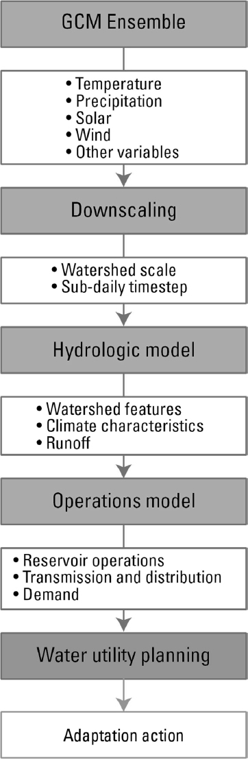
One way for the OST to be used as a planning tool for climate change is for it to be exercised in a chain-of-models approach (Figure B-1) (Vogel et al., 2016). To characterize how a changing climate may affect hydrologic processes and water resources at regional scales, many studies utilize downscaled projections of future temperature and precipitation from global climate models to drive hydrologic models to estimate impacts on streamflow, sediments, and pollutants at the watershed scale. This appendix describes some of the models and methods for the first three components of this approach—global climate models (GCMs), downscaling techniques, and hydrologic models—highlighting the associated challenges in projecting future impacts on water resources through the use of linked GCMs and hydrologic models. Operations models and water utility planning are considered in following sections.
GLOBAL CLIMATE MODELS
A GCM is a mathematical representation of the behavior of Earth’s climate system over time that can be used to estimate the sensitivity of the climate system to changes in atmospheric concentrations of greenhouse gases and aerosols (Horton et al., 2015). How atmospheric greenhouse gases may change in the future is characterized by a set of representative concentration pathways (RCPs) (Moss et al., 2010). These numerical models, originally known as general circulation models and now commonly known as global climate models, mathematically represent physical processes in the atmosphere, ocean, cryosphere, and land
surface and their interactions and feedbacks (IPCC, 2013a). Comprehensive GCMs known as coupled atmosphere-ocean models (AOGCMs) are advanced tools for simulating the response of the global climate system to increasing greenhouse gas concentrations in the coming decades to centuries. Because of the complicated physics and chemistry represented in the GCM, their atmospheric spatial resolution across the models used in CMIP51 ranges from ~1 to 2.5 degrees with higher resolution over the oceans. Land resolution tends to be the same as the atmospheric resolution.
DOWNSCALING
In order for outputs from coarse-scale GCMs to be used in finer-scale hydrologic watershed models, results must be downscaled. Downscaling to the catchment scale can be accomplished through RCMs that use the GCM as boundary conditions for the simulated regions. The Coordinated Regional Downscaling Experiment (CORDEX) is coordinated by the World Climate Research Program (WCRP) of which the North American CORDEX (NA-CORDEX) data archive contains output from RCMs run over a domain covering most of North America using boundary conditions from GCM simulations in the CMIP5 archive.2 These simulations run from 1950 to 2100 with a spatial resolution of 0.22°/25 km or 0.44°/50 km with data available for impact-relevant variables at daily and longer frequencies. One significant challenge with CORDEX-based simulations is the use of GCM output for the boundary conditions, since biases in the GCM will impact the RCM. Correcting these boundary conditions is extremely problematic, and so a feasible approach is to bias-correct the RCM outputs using observed meteorology before their use as inputs to hydrologic models (e.g., Yang et al., 2010).
Alternatively, a range of statistical approaches (e.g., Fu et al., 2013; Schnorbus et al., 2014; Wang et al., 2014) can be used that includes historical relationships between coarse-scale GCM grids and fine-scale hydrologic modeling grids. These relationships are then assumed to hold for future climate conditions. Statistical approaches were widely used before NA-CORDEX simulations were made widely available. Using a combination of RCM with statistical bias correction may offer the best combination, since the RCM offers a 25-km resolution such that further downscaling to hydrologic scales, say 10 km, limits the scale mismatch.
___________________
1 Under the World Climate Research Programme, the Working Group on Coupled Modelling established the Coupled Model Intercomparison Project (CMIP) as a standard experimental protocol for studying the output of AOGCMs. CMIP provides a community-based infrastructure in support of climate model diagnosis, validation, intercomparison, documentation, and data access. CMIP5 is the fifth phase of the intercomparison.
2 See https://na-cordex.org.
Regional Climate Models
RCMs are limited-area models with representations of climate processes comparable to those in the atmospheric and land surface components of AOGCMs, though typically run without interactive ocean and sea ice (Flato et al., 2014). RCMs are often used to dynamically downscale global model simulations for a particular geographic region to provide more detailed information (Laprise, 2008; Rummukainen, 2010).
With finer resolution, RCMs can resolve mesoscale phenomena that contribute to intense precipitation, such as stronger upward motions (Jones et al., 1995) and coupling between regional circulation and convection (e.g., Anderson et al., 2007). They can reveal more intense rain events that would be smoothed over in coarser-resolution GCMs. The higher resolution of RCMs also enables the simulation of short-term variability such as extreme winds and locally extreme temperatures that are not captured in coarser-resolution models.
RCMs can resolve sharp differences in topography and their influence on precipitation processes such as rain shadows, which require the resolution of surface features finer than the typical coarse GCM resolution (e.g., Leung and Wigmosta, 1999; Hay et al., 2006). RCMs also simulate the climatic influences of bodies of water, their downstream influences, and such phenomena as sea breezes (e.g., Anderson et al., 2001; Lofgren, 2004). RCMs use boundary conditions from the output of coarser-scale GCMs and as such, large-scale biases derived from errors in the GCM may be introduced into the RCM projections.
Empirical/Statistical Downscaling, Bias Correction, and Delta Method
Empirical or statistical downscaling is another approach to obtaining regional-scale climate information (Hewitson and Crane, 1996; Kattenberg et al., 1996; Giorgi et al., 2001; Wilby et al., 2004). It uses statistical relationships to relate the coarse-scale GCM predictions to observed climate within the GCM grid (in a targeted area). The targeted area’s size can be as small as a single point. As long as significant statistical relationships exist, empirical downscaling can yield regional information for any desired variable such as precipitation and temperature, although care must be taken when downscaling multiple variables in order to maintain correlations.
This approach encompasses a range of statistical techniques from simple linear regression (e.g., Wilby et al., 2000) to more-complex applications such as those based on weather generators (Wilks and Wilby, 1999), canonical correlation analysis (e.g., von Storch et al., 1993), or artificial neural networks (e.g., Crane and Hewitson, 1998). Empirical downscaling can be inexpensive compared to numerical simulation when applied to just
a few locations or when simple techniques are used. Lower costs, together with flexibility in targeted variables, have led to a wide variety of applications for assessing impacts of climate change (CCSP, 2008).
One statistical downscaling technique is the constructed analogue approach (Van den Dool, 1994; Hidalgo et al., 2008), which uses observed coarse-scale observations and generates a relationship between the observed weather patterns and daily GCM patterns at a coarse scale; this relationship is then translated to a finer scale to produce regional information.
Bias correction is a standard practice to correct the projected “raw” daily GCM output using the differences in the mean and variability between GCM and observations in a reference period (IPCC, 2013a). The delta method is a frequently applied type of bias correction whereby the difference between each model’s future and baseline simulation is employed rather than direct model outputs (Gleick, 1986; Wilby et al., 2004; Horton et al., 2011). Long-term changes from climate model outputs are considered more reliable than individual values, especially when the target area is smaller than the size of a climate model grid box for which the calculations are made. These changes are then applied to observed time series to create climate change scenarios for use in impact models. Recent examples of this type of study include Fan and Shibata (2015). The differences and ratios are also applied to stochastic weather generators in some studies.
Bias correction and spatial disaggregation (BCSD) (Wood et al., 2002; Ahmed et al., 2013) is a downscaling method in wide use. The BCSD approach first adjusts the output from the GCMs to account for tendencies in the model to be too wet, dry, warm, or cool during the historical period (bias correction), and then the adjusted data are converted to regional data for spatial downscaling. This results in simulated future conditions in which the temporal pattern of precipitation is identical to the historical pattern; that is, the duration and time between events are unchanged. The only thing that changes is the intensity of precipitation within the events.
The challenges of downscaling and bias correction, through either RCMs, statistical methods, or a combination of approaches, led to the Chapter 5 recommendation that is repeated here: the NYC DEP should establish selection criteria for GCMs used as inputs based on how well the GCMs reproduce current climate and major climate trends over recent decades in this region. By starting with GCM models for which historical predictions reflect such attributes as annual patterns of monthly mean temperature, precipitation, and runoff for the region and daily predictions of hydrologic variables important for extreme-event analysis, the chances of accurate downscaling are improved.
HYDROLOGIC WATERSHED MODELS
To project climate change impacts to a watershed scale, downscaled temperature and precipitation data are used as input to hydrologic models to determine such parameters as streamflow, runoff, and infiltration. Standard hydrologic models, such as the Soil Water Assessment Tool (SWAT), Hydrological Simulation Program—FORTRAN (HSPF), Variable Infiltration Capacity (VIC) model, and the Generalized Watershed Loading Function (GWLF), have been used in climate change studies. The NYC DEP has used the SWAT and GWLF models in some of its climate change studies (Matonse et al., 2011; Mukundan et al., 2013). These watershed models simulate such processes and components as the soil water balance (including runoff, infiltration, and evapotranspiration), unsaturated subsurface water, saturated groundwater and groundwater flow, and exchanges between surface water and groundwater (Vazquez-Amábile and Engel, 2005; Daniel et al., 2011; Demaria et al., 2016). With regard to water quality, the models simulate erosion and sediment, nutrient, and pesticide transport in the designated domain.
LIMITATIONS OF CLIMATE AND HYDROLOGIC MODELS
The chain-of-models approach is subject to limitations since each of the individual elements has its own associated weaknesses, which are then concatenated as the models are used in series. This is known as the uncertainty cascade (Wilby, 2017). We highlight here issues related to global and regional climate models, downscaling techniques, and hydrologic models.
Global Climate Model Limitations
GCMs, at the head of the chain, are subject to several types of uncertainty. The sources of uncertainty in climate models stem from lack of knowledge about future concentrations of greenhouse gases, sensitivity of the climate system, regional and local changes, and natural variability (Horton et al., 2015). Feedback mechanisms, such as those due to the effects of changes in ice and snow on albedo and the climate system, as well as changes in water vapor and its effects on warming, are active research areas. The current generation of climate models tends to imperfectly simulate extreme events due to limitations of model resolution and representation of relevant physical mechanisms (Bellprat and Doblas-Reyes, 2016).
A crucial issue is that when GCMs are decoupled from hydrologic models (as is the case with the model chain approach described here), the results can be in error due to incorrect estimates of evapotranspiration. As a result, changes in runoff are typically projected to be much more
extreme than is realistic if modeled in a fully coupled mode (Milly and Dunne, 2011, 2017). Differences in formulations for hydrologic variables, especially evapotranspiration, between GCMs and hydrologic models cause differences in projected changes in runoff. These findings highlight the need for caution when projecting changes in evapotranspiration for use in hydrologic models or drought indices to evaluate climate change impacts on water resources.
Demaria et al. (2016) on the other hand found that structural biases in the hydrological models and uncertainty in the bias correction–temporal disaggregation process can contribute to underestimation of streamflow extreme highs, which implies that mid-century projected positive trends can be a conservative estimate of their magnitude.
Many processes occur at finer temporal and spatial scales than GCMs can resolve. GCMs instead approximate how these processes function at the coarser scale that the model can resolve using empirical equations, or parameterizations, based on a combination of observations and scientific understanding. Examples of important processes that are parameterized in climate models include turbulent mixing, heating/cooling by radiation, and small-scale physical processes such as cloud formation and precipitation, chemical reactions, and exchanges between the biosphere and atmosphere. For example, GCMs cannot represent realistic rainfall. Instead, they simulate the total amount of rain that would fall over a large area the size of a grid cell in the model. These approximations are usually derived from a limited set of observations and/or coarser-resolution modeling and may not hold true for every location or under all possible conditions (Walsh et al., 2014).
By providing projections that span a range of global climate models and greenhouse gas emissions trajectories, global climate change uncertainties may be better characterized, but they cannot be fully eliminated (Horton et al., 2010). Averaging projections over 30-year time slices and showing changes in climate through time rather than absolute climate values reduces regional-scale uncertainties, although it does not address the possibility that regional climate processes may change with time in ways that are not captured by the global climate models. At the regional scale, even the selection of all the available GCM experiments would not guarantee a representative range, due to the processes that GCMs do not fully address (IPCC, 2013b).
Regional Climate Model Limitations
As previously mentioned, an important limitation for regional climate model simulations is that they are dependent on boundary conditions supplied from other sources, often GCMs (CCSP, 2008). Thus, regional simulations by RCMs are dependent on the model quality or on observa-
tions supplying boundary conditions. This is especially true for projections of future climate, suggesting value in performing an ensemble of simulations using multiple atmosphere-ocean global models to supply boundary conditions, thus including some of the uncertainty involved in constructing climate models and projecting future changes in boundary conditions. With regard to statistical downscaling, it should be noted that this method does not reduce the uncertainty in GCM projections. This makes the use of RCMs an attractive alternative for future studies as they become more widely available (Liang et al., 2012).
Bias Correction Limitations
There are important limitations in the bias correction methods previously described. The ratio method for precipitation ensures that the coefficient of variation of daily precipitation amounts on days with rain, and the duration of rain-free and rainy periods, are unchanged from the historical period. Yet the current thinking is that both of these things are likely to change substantially in the future. Further, BCSD corrects biases in mean levels, but does not address biases in trends.
Hydrologic Model Limitations
Rigorous validation is essential when using hydrologic models to ensure that they represent past and current conditions appropriately (Demaria et al., 2016). For assessment of future conditions, hydrologic models often assume that the vegetation cover is static in time; therefore, the interaction between vegetation and snow might not be realistically represented in the future. Furthermore, hydrologic models often assume model transportability in time, that is, that the parameter calibration will be valid under different climatic conditions.
REFERENCES
Ahmed, K. F., G. Wang, J. Silander, A. M. Wilson, J. M. Allen, R. Horton, and R. Anyah. 2013. Statistical downscaling and bias correction of climate model outputs for climate change impact assessment in the US Northeast. Global and Planetary Change 100:320–332.
Anderson, B. T., J. O. Roads, S. C. Chen, and H. M. H. Juang. 2001. Model dynamics of summertime low-level jets over northwestern Mexico. Journal of Geophysical Research: Atmospheres 106(D4):3401–3413.
Anderson, C. J., R. W. Arritt, and J. S. Kain. 2007. An alternative mass flux profile in the Kain-Fritsch convective parameterization and its effects in seasonal precipitation. Journal of Hydrometeorology 8(5):1128–1140.
Bellprat, O., and F. Doblas-Reyes. 2016. Attribution of extreme weather and climate events overestimated by unreliable climate simulations. Geophysical Research Letters 43:2158–2164.
CCSP (Climate Change Science Program). 2008. Climate Models: An Assessment of Strengths and Limitations. Washington, DC: U.S. Department of Energy, Office of Biological and Environmental Research. https://science.energy.gov/~/media/ber/pdf/Sap_3_1_final_all.pdf.
Crane, R. G., and B. C. Hewitson. 1998. Doubled CO2 precipitation changes for the Susquehanna basin: Down-scaling from the GENESIS general circulation model. International Journal of Climatology 18:65–76.
Daniel, E. B., J. V. Camp, E. J. LeBoeuf, J. R. Penrod, J. P. Dobbins, and M. D. Abkowitz. 2011. Watershed modeling and its applications: A state-of-the-art review. Open Hydrology Journal 5:26–50.
Demaria, E. M., R. N. Palmer, and J. K. Roundy. 2016. Regional climate change projections of streamflow characteristics in the Northeast and Midwest US. Journal of Hydrology: Regional Studies 5:309–323.
Fan, M., and H. Shibata. 2015. Simulation of watershed hydrology and stream water quality under land use and climate change scenarios in Teshio River watershed, northern Japan. Ecological Indicators 50:79–89.
Flato, G., J. Marotzke, B. Abiodun, P. Braconnot, S. C. Chou, W. Collins, P. Cox, F. Driouech, S. Emori, V. Eyring, C. Forest, P. Gleckler, E. Guilyardi, C. Jakob, V. Kattsov, C. Reason, and M. Rummukainen. 2014. Evaluation of climate models. In: Climate Change 2013: The Physical Science Basis. Contribution of Working Group I to the Fifth Assessment Report of the Intergovernmental Panel on Climate Change, T. F. Stocker, D. Qin, G.-K. Plattner, M. Tignor, S. K. Allen, J. Boschung, A. Nauels, Y. Xia, V. Bex, and P. M. Midgley (eds.). Cambridge, UK and New York: Cambridge University Press, pp 741–866.
Fu, G., S. P. Charles, F. H. Chiew, J. Teng, H. Zheng, A. J. Frost, W. Liu, and S. Kirshner. 2013. Modelling runoff with statistically downscaled daily site, gridded and catchment rainfall series. Journal of Hydrology 492:254–265.
Giorgi, F., B. Hewitson, J. Christensen, M. Hulme, H. Von Storch, P. Whetton, R. L. Jones, L. Mearns, C. Fu, and R. Arritt. 2001. Regional climate change information—Evaluation and projections. In: Climate Change 2001: The Scientific Basis. Contribution of Working Group I to the Third Assessment Report of the Intergovernmental Panel on Climate Change, J. T. Houghton, Y. Ding, D. J. Griggs, M. Noguer, P. J. van der Linden, X. Dai, K. Maskell, and C.A. Johnson (eds.). Cambridge, UK: Cambridge University Press, pp. 583–638.
Gleick, P. H. 1986. Methods for evaluating the regional hydrologic impacts of global climatic changes. Journal of Hydrology 88(1-2):97–116.
Hay, L. E., M. P. Clark, M. Pagowski, G. H. Leavesley, and W. J. Gutowski, Jr. 2006. One-way coupling of an atmospheric and a hydrologic model in Colorado. Journal of Hydrometeorology 7:569–589.
Hewitson, B. C., and R. G. Crane. 1996. Climate downscaling: Techniques and application. Climate Research 7:85–95.
Hidalgo, H. G., M. D. Dettinger, and D. R. Cayan. 2008. Downscaling with Constructed Analogues: Daily Precipitation and Temperature Fields over the United States. PIER Final Project Report CEC-500-2007-123. Sacramento: California Energy Commission.
Horton, R., V. Gornitz, M. Bowman, and R. Blake. 2010. Ch. 3: Climate observations and projections. In: Annals of the New York Academy of Sciences 1196:41–62. doi:10.1111/j.1749-6632.2009.05314.x
Horton, R. M., V. Gornitz, D. A. Bader, A. C. Ruane, R. Goldberg, and C. Rosenzweig. 2011. Climate hazard assessment for stakeholder adaptation planning in New York City. Journal of Applied Meteorology and Climatology 50(11):2247–2266.
Horton, R., D. Bader, Y. Kushnir, C. Little, R. Blake, and C. Rosenzweig. 2015. Chapter 1: Climate observations and projections. In: New York City Panel on Climate Change 2015 Report. Annals of the New York Academy of Sciences 1336:18–35. doi:10.1111/nyas.12586.
IPCC (Intergovernmental Panel on Climate Change). 2013a. Climate Change 2013: The Physical Science Basis. Contribution of Working Group I to the Fifth Assessment Report of the Intergovernmental Panel on Climate Change. New York: Cambridge University Press.
IPCC. 2013b. What Is a GCM? http://www.ipcc-data.org/guidelines/pages/gcm_guide.html.
Jones, R. G., J. M. Murphy, and M. Noguer. 1995. Simulation of climate change over Europe using a nested regional climate model. Part I: Assessment of control climate, including sensitivity to location of lateral boundaries. International Journal of Climatology 121:1413–1449.
Kattenberg, A., F. Giorgi, H. Grassl, G. A. Meehl, J. F. B. Mitchell, R. J. Stouffer, T. Tokioka, A. J. Weaver, and T. M. L. Wigley. 1996. Climate models—Projections of future climate. In: Climate Change 1995–The Science, J. T. Houghton, L. G. Meiro Filho, B. A. Callander, N. Harris, A. Kattenburg, and K. Maskell (eds.). Cambridge, UK: Cambridge University Press, pp. 285–358.
Laprise, R. 2008. Regional climate modelling. Journal of Computational Physics 227(7): 3641–3666.
Leung, L. R., and M. S. Wigmosta. 1999. Potential climate change impacts on mountain watersheds in the Pacific Northwest. Journal of the American Water Resources Association 35:1463–1471.
Liang, X. Z., M. Xu, X. Yuan, T. Ling, H. I. Choi, F. Zhang, L. Chen, S. Liu, S. Su, F. Qiao, and Y. He. 2012. Regional climate–Weather research and forecasting model. Bulletin of the American Meteorological Society 93(9):1363–1387.
Lofgren, B. M. 2004. A model for simulation of the climate and hydrology of the Great Lakes basin. Journal of Geophysical Research 109(D18):D18108; doi:10.1029/2004JD004602.
Matonse, A. H., D. C. Pierson, A. Frei, M. S. Zion, E. M. Schneiderman, A. Anandhi, R. Mukundan, and S. M. Pradhanang. 2011. Effects of changes in snow pattern and the timing of runoff on NYC water supply system. Hydrological Processes 25(21):3278–3288.
Milly, P. C., and K. A. Dunne. 2011. On the hydrologic adjustment of climate-model projections: The potential pitfall of potential evapotranspiration. Earth Interactions 15(1):1–14.
Milly, P. C. D., and K. A. Dunne. 2017. A hydrologic drying bias in water-resource impact analyses of anthropogenic climate change. Journal of the American Water Resources Association 53(4):822–838.
Moss, R. H., J. A. Edmonds, K. A. Hibbard, M. R. Manning, S. K. Rose, D. P. Van Vuuren, T. R. Carter, S. Emori, M. Kainuma, T. Kram, and G. A. Meehl. 2010. The next generation of scenarios for climate change research and assessment. Nature 463(7282):747–756.
Mukundan, R., S. M. Pradhanang, E. M. Schneiderman, D. C. Pierson, A. Anandhi, M. S. Zion, A. H. Matonse, D. G. Lounsbury, and T. S. Steenhuis. 2013. Suspended sediment source areas and future climate impact on soil erosion and sediment yield in a New York City water supply watershed, USA. Geomorphology 183:110–119.
Rummukainen, M. 2010. State-of-the-art with regional climate models. Wiley Interdisciplinary Reviews: Climate Change 1(1):82–96.
Schnorbus, M., A. Werner, and K. Bennett. 2014. Impacts of climate change in three hydrologic regimes in British Columbia, Canada. Hydrological Processes 28(3):1170–1189.
Van den Dool, H. M. 1994. Searching for analogues, how long must we wait? Tellus A: Dynamic Meteorology and Oceanography 46(3):314–324.
Vazquez-Amábile, G., and B. A. Engel. 2005. Use of SWAT to compute groundwater table depth and streamflow in Muscatatuck River watershed. Transactions of the American Society of Agricultural Engineers 48:991–1003.
Vogel, J., E. Mcnie, and D. Behar. 2016. Co-producing actionable science for water utilities. Climate Services 2–3:30–40.
von Storch, H., E. Zorita, and U. Cubasch. 1993. Downscaling of global climate change estimates to regional scales: An application to Iberian rainfall in wintertime. Journal of Climate 6(6):1161–1171.
Walsh, J., D. Wuebbles, K. Hayhoe, J. Kossin, K. Kunkel, G. Stephens, P. Thorne, R. Vose, M. Wehner, J. Willis, D. Anderson, V. Kharin, T. Knutson, F. Landerer, T. Lenton, J. Kennedy, and R. Somerville. 2014. Appendix 3: Climate science supplement. In: Climate Change Impacts in the United States: The Third National Climate Assessment, J. M. Melillo, T. C. Richmond, and G. W. Yohe (eds.). U.S. Global Change Research Program, pp. 735–789. doi:10.7930/J0KS6PHH.
Wang, R., L. Kalin, W. Kuang, and H. Tian. 2014. Individual and combined effects of land use/cover and climate change on Wolf Bay watershed streamflow in southern Alabama. Hydrological Processes 28(22):5530–5546.
Wilby, R. L. 2017. Climate Change in Practice: Topics for Discussion with Group Exercises. Cambridge, UK: Cambridge University Press.
Wilby, R. L., L. E. Hay, W. J. Gutowski, R. W. Arritt, E. S. Takle, Z. Pan, G. H. Leavesley, and M. P. Clark. 2000. Hydrological responses to dynamically and statistically downscaled climate model output. Geophysical Research Letters 27(8):1199–1202.
Wilby, R. L., S. P. Charles, E. Zorita, B. Timbal, P. Whetton, and L. O. Mearns. 2004. Guidelines for Use of Climate Scenarios Developed from Statistical Downscaling Methods. Intergovernmental Panel on Climate Change. http://www.ipcc-data.org/guidelines/dgm_no2_v1_09_2004.pdf.
Wilks, D. S., and R. L. Wilby. 1999. The weather generation game: A review of stochastic weather models. Progress in Physical Geography 23(3):329–357.
Wood, A. W., E. P. Maurer, A. Kumar, and D. Lettenmaier. 2002. Long-range experimental hydrologic forecasting for the eastern United States. Journal of Geophysical Research 107(D20):4429; doi:10.1029/2001JD000659.
Yang, W., J. Andréasson, L. P. Graham, J. Olsson, J. Rosberg, and F. Wetterhall. 2010. Distribution-based scaling to improve usability of regional climate model projections for hydrological climate change impacts studies. Hydrology Research 41(3–4):211–229.
This page intentionally left blank.


