
A
Observed Hydrologic Trends
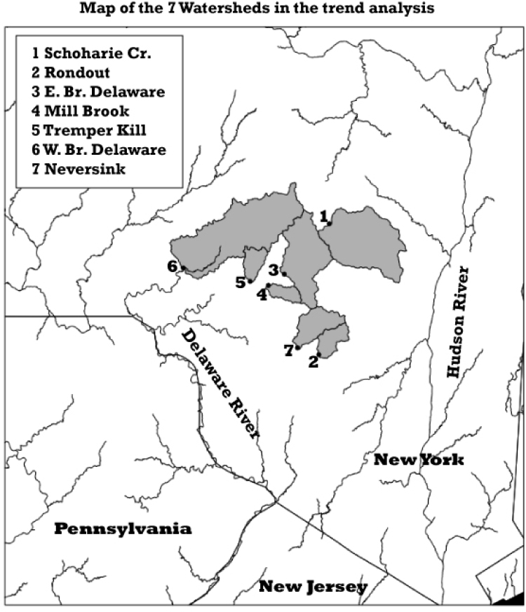
Chapters 2 and 5 both raise issues about the need to use recent (e.g., last two decades of) hydrologic or climatic data in various uses of the Operations Support Tool (OST). In Chapter 2, the concern is raised about the fact that the ensemble forecasts used in the position analysis (PA) applications of OST do not make full use of the most recent parts of the record. Chapter 5 discusses the idea of using recent hydrologic trends as one possible indicator of future trends. Given the potential importance of observed recent trends to both the OST PA application for current operations and to the OST simulation (Sim) application for climate change sensitivity studies, the Committee embarked on a small exploratory analysis of the actual hydrologic records for example watersheds from across the New York City watershed region. The analyses presented here are based on long-term streamflow data collected by the USGS from a set of seven U.S. Geological Survey (USGS) streamgages, all of which have been operated since 1950 and continue to be operated up to the present. All seven of these are considered to be reference gages because they have no significant upstream reservoirs regulating the flow and no major centers of population upstream. Thus, the observed changes in streamflow at these gages are probably largely influenced by trends in climate but they could also be influenced by trends in land use. The locations of these streamgages and their watersheds are shown in Figure A-1.
The analysis is based on the 21,407 daily streamflow values covering the time span of December 1, 1951, through November 30, 2017, for each of the seven streamgages. The data were downloaded from the USGS National Water Information System using the EGRET R package (Hirsch
and De Cicco, 2015). The data sets were divided into four seasons: winter, consisting of December, January, and February; spring, consisting of March, April, and May; summer, consisting of June, July, and August; and fall, consisting of September, October, and November. For each of these four seasons, the analysis explored the trends at each streamgage for two variables: mean seasonal discharge and one-day maximum discharge per season.
MEAN SEASONAL DISCHARGE
The first variable considered is the mean discharge for each season for each of the 66 years in the data set. This information can help identify any substantial trends in streamflow over the record and compare trends in different parts of the year. Of particular interest is the question of changes in timing associated with the ongoing shift in relative importance of snow versus rain in the hydrology of the region. Also of interest are the streamflow values observed in the drier parts of the year (summer and fall); delivery of water from the reservoirs during this low-flow season is a critical function of the reservoir system. Declines in streamflow during these seasons could affect the ability of the water supply reservoirs to meet customer demand. Decreases in streamflow in these seasons could lead to a decrease in the reliability of the supply, an important metric of system performance.
The analysis starts by considering the trends in seasonal mean flows for one of the seven streamgages, Schoharie Creek at Prattsville, New York. This streamgage measures the outflow of the second largest of these seven watersheds (an area of 613 km2) and has among the largest observed summer trends of any of the seven. Figure A-2 shows the record for the summer season (June, July, and August).
The dots indicate the observed mean discharge for the summer months of each of the 66 years in the record. The curve is a smoothed representation of the data shown on the graph (for details of the smoothing method see Hirsch and DeCicco, 2015, pp. 16–18). At the top of each graph

is shown the results of a nonparametric trend test: the Mann-Kendall test (Mann, 1945; Kendall, 1975). The significance levels (p-values) are modified to account for the existence of serial correlation, using a method developed by Zhang et al. (2001) and implemented with the zyp R package (Bronaugh and Werner, 2013). A p-value less than 0.05 is generally considered to be an indication that the trend is statistically significant. In this case, p = 0.0288, indicating that a monotonic trend of this magnitude or greater (in absolute value) has a probability of 0.0288 if the data were a sample from a trend-free random variable. The magnitude of the trends is estimated using the Thiel-Sen (Sen, 1968) slope estimator, a nonparametric slope estimate, closely related to the Mann-Kendall test. The trends are expressed in units of percent per year. Because the trends were computed on the logarithm of the actual values, one can translate annual trend to a total amount of change over the entire 66-year period. The trend estimate here translates to a total change of 133 percent over the entire record.
Shifting our analysis to the spring months of March, April, and May, one gets a very different result, shown in Figure A-3.
The results for the spring season are quite different from the summer season. The analysis indicates a virtually trend-free history over this period with a slight indication of a downward trend over the past 20 years, but
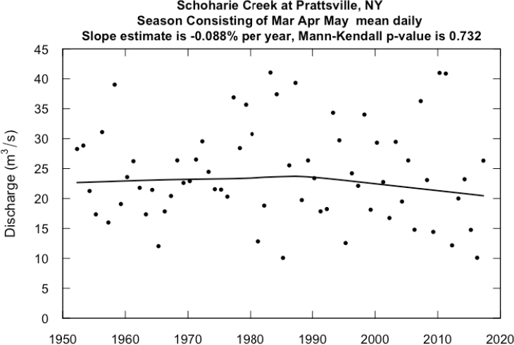
overall the change for the period is a 5.5 percent decrease and it is not even close to being significant (p = 0.732).
The purpose of this analysis is simply to quantify the trends that have taken place and compare the differences across seasons, not to determine the cause of the observed trends. Also, it is useful to determine if the trends are relatively similar across the New York City watershed region or if they are substantially different among the different watersheds. The summer increase at all of the sites is primarily focused on the period 1970 to present, which coincides with the start of the rapid increase in greenhouse gas concentrations. Thus, it is plausible that the change in summer streamflow is caused by changes in global greenhouse forcing. Although the linkage is not proven by this analysis, it does suggest that projections of future streamflow conditions should consider the possibility that summer streamflows will continue to increase as greenhouse gas concentrations continue to increase. Land-use change is another plausible explanation, but given the fact that there are strong land-use controls within the New York City watershed it seems an unlikely explanation. However, these two possible options (climate and land use) as explanations for the change would be an appropriate subject for the NYC DEP to explore. Regardless of the cause of this substantial trend since 1970, it is important that planning and operational simulations take note of this change in the hydrology of the New York City watershed. Table A-1 gives the results for all four seasons for all seven streamgages. On the table, the change over the past 66 years is shown in percent.
Table A-1 shows that the changes in streamflow are very consistent across all seven of these watersheds. The largest and most statistically significant changes were for the summer months and all of them were increases. The next largest changes were in the fall months, and although none of them could be considered significant, they are also increases. The spring season had small decreases, generally not significant, and the winter had small increases that were also generally not significant. These findings are generally good news from a water supply reliability standpoint, showing that over the past 66 years, the mean streamflow in the drier two seasons of the year has increased, and the only season showing a decrease was the spring, but that change was quite small and generally not statistically significant. Formal analysis, using OST in Sim mode, could be undertaken to further analyze the implications of these trends. For example, one could “detrend” the historic streamflow record to adjust it to conditions that were more typical of the 1950s and then run them through OST in Sim mode. They could also be detrended and adjusted to conditions more typical of the 2010s and then run through OST in Sim mode. Frequencies of low storage, or of failure to deliver water to meet customer demand, could be compared across these two simulations, to gain some understanding of how reliability
TABLE A-1 Results of the Mann-Kendall Test for Monotonic Trend in Daily Mean Discharge for the Season, at Seven Reference Streamgages in the New York City Watershed Area, for Each of Four Seasons, 1951–2017
| Streamgage Name | Site # | Drainage km2 | Winter (DJF) Change in % | Spring (MAM) Change in % | Summer (JJA) Change in % | Fall (SON) Change in % |
|---|---|---|---|---|---|---|
| Schoharie Creek at Prattsville, NY | 1350000 | 613 | 28 | –6 | 139** | 88 |
| Rondout Creek near Lowes Corners, NY | 1365000 | 99 | 40* | –14 | 154*** | 86 |
| East Branch Delaware River at Margaretville, NY | 1413500 | 422 | 27 | –11 | 137*** | 86 |
| Mill Brook near Dunraven, NY | 1414500 | 65 | 14 | –20* | 130*** | 64 |
| Tremper Kill near Andes, NY | 1415000 | 85 | 20 | –12 | 155*** | 57 |
| West Branch Delaware River at Walton, NY | 1423000 | 859 | 33 | –5 | 106** | 75 |
| Neversink River near Claryville, NY | 1435000 | 172 | 32* | –15 | 100** | 68 |
NOTES: The change over the period is expressed as a percentage change over the period. The significance level of the change is indicated as follows: *** if the test is significant with p < 0.01, ** if the test is significant with p in the range 0.05 to 0.01, and * if the test is significant with p in the range 0.1 to 0.05. No asterisk indicates it is not significant (p > 0.1). DJF = December, January, February. MAM = March, April, May. JJA = June, July, August. SON = September, October, November.
may have changed over time. A third simulation option would be to take the historic record and adjust it to have trends going forward that simply extend the recent rates of change (for example, from the past 40 years) into the future an additional 80 years.
ONE-DAY MAXIMUM DISCHARGE PER SEASON
The same historic streamflow record was examined in terms of the one-day maximum discharge for each season of each year. The one-day maximum is important because these high flows are the triggers for high-turbidity events, which are a crucial driver of system operations. If, for example, one found that these one-day maximum discharges were becoming larger over time (presumably as a result of enhanced greenhouse forcing), then prudent management of the system would lead to maintaining lower storage levels in those watersheds prone to high turbidity, so that these high-turbidity events could be captured and particulate matter allowed to settle before delivering water to Kensico Reservoir. All other things being equal, this would have an adverse effect on system reliability, because it would decrease the capacity of the system to store water in the wet seasons to satisfy potential needs in drier seasons.
Figure A-4 shows the results of the analysis for the summer season for Schoharie Creek. Note the difference in the vertical scale for discharge compared to Figure A-2.
Figure A-4 is interesting because the record shows the size of the 2011 event, the peak day discharge from Hurricane Irene. This daily discharge
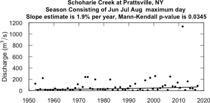
of about 1,130 m3/s is not only unprecedented in this 66-year period of summer values, but is actually the largest daily discharge in any season in the entire century-long discharge record (exceeding the second largest by more than 50 percent). But, one large value does not make a trend. The Mann–Kendall test is designed to be resistant to extreme values, and thus, while it recognizes that the largest value in this record occurs in the last few years of the record, it is not sensitive to the particularly large value that was observed. Rather, the trend test is responsive to the bulk of the data.
Another notable feature of this record is the increased frequency of values above about 150 m3/s in the last 20 to 25 years of this record; the trend test result is mostly responsive to changes of that kind. One can conclude that summer season maximum daily discharges do seem to have increased in size over the 66-year period. The result is significant (p = 0.0345) and the trend, over the 66-year record, is + 239 percent. The results for seasonal one-day maximum discharge across all four seasons and all seven sites are shown in Table A-2.
These results are generally similar to those shown in Table A-1 (for seasonal mean discharge). The summer season shows very large and generally significant increases in maximum one-day discharges. The fall shows increases as well, but smaller than summer and not significant at any of the seven streamgages. The winter and spring seasons had a mixture of small positive and negative changes, none of which was significant. The summer and fall increases are consistent with findings about increases in summer intense precipitation (from a variety of storm types, including tropical storms).
In contrast with the results about mean flows, these results about maximum flows are potentially problematic for the New York City watersheds, because it appears that streamflow events conducive to high-turbidity inputs are becoming more frequent and larger in size, at least in the summer. To integrate these findings with those about mean flows, these findings could be used to further modify the historic record by specifically detrending the most extreme discharges as well as detrending the seasonal average discharges to create artificial records that could serve as inputs to OST operated in Sim mode. The question that could be posed might be of the following form: If we project recent trends in mean flows, and recent trends in peak flows, into the future and then run them through OST in Sim mode, do they indicate increases in the frequency or severity of turbidity violations at Kensico and/or increases in the frequency or severity of shortages of water delivered to customers?
None of these trend results or related simulations can deliver a simple answer to questions of future changes in overall system reliability or questions about the need for changes in system operation. The point here is really one of applying adaptive management principles: using the observations going forward to evaluate likely changes in system performance and then
TABLE A-2 Results of the Mann-Kendall Test for Monotonic Trend in the One-Day Maximum Discharge, at Seven Reference Streamgages in the New York City Watershed Area, for Each of Four Seasons, 1951–2017
| Streamgage Name | Site # | Drainage km2 | Winter (DJF) Change in % | Spring (MAM) Change in % | Summer (JJA) Change in % | Fall (SON) Change in % |
|---|---|---|---|---|---|---|
| Schoharie Creek at Prattsville, NY | 1350000 | 614 | 38 | 16 | 239** | 112 |
| Rondout Creek near Lowes Corners, NY | 1365000 | 99 | 38 | –11 | 307*** | 70 |
| East Branch Delaware River at Margaretville, NY | 1413500 | 422 | 1.7 | –4.5 | 210** | 97 |
| Mill Brook near Dunraven, NY | 1414500 | 65 | –11 | –15 | 181** | 100 |
| Tremper Kill near Andes, NY | 1415000 | 86 | –28 | –4.4 | 138* | 68 |
| West Branch Delaware River at Walton, NY | 1423000 | 860 | –18 | 16 | 148* | 88 |
| Neversink River near Claryville, NY | 1435000 | 172 | 50 | –12 | 135 | 116 |
NOTES: The change over the period is expressed as a percentage change over the period. The significance level of the change is indicated as follows: *** if the test is significant with p < 0.01, ** if the test is significant with p in the range 0.05 to 0.01, and * if the test is significant with p in the range 0.1 to 0.05. No asterisk indicates it is not significant (p > 0.1). DJF = December, January, February. MAM = March, April, May. JJA = June, July, August. SON = September, October, November.
feeding back the insights into management changes, either through changes in infrastructure or changes in the operational parameters of OST.
COMPARISON OF THE HYDROLOGY OF 1950–1997 VERSUS 1998–2017
One final analysis was conducted that is related to the concern expressed in Chapter 2 about the fact that the historical weather information used in parts of the the Hydrologic Ensemble Forecasting Service (HEFS) system uses data from 1950 to 1997 rather than from 1950 to 2017. Even if climate were, in fact, stationary, there still would be some reason for concern about the absence of the last 20 years of data because estimates based on longer records can be expected to be more accurate (simply because of the increase in the sample size). But, if one adds in ongoing changes in the climate and resulting changes in hydrology, then concern about the absence of data from the past two decades becomes even more serious. To address this question in a simple, data-driven manner, the Committee explored the empirical probability distribution of daily streamflows from two different periods using the Schoharie Creek data previously described.
The period currently being used by OST (water years 1950–1997) has a mean discharge of 13.35 m3/s. The more recent period (water years 1998–2017) has a mean discharge of 15.33 m3/s. So, the period being used in the OST simulations has a mean that is 13 percent below the mean for the more recent period.
What is the importance of this set of results? First, the more recent years that are not used in HEFS are distinctly higher in discharge than the set of years that are used. This suggests that operational estimates of probability distributions will represent conditions from a period of lower overall discharge than what recent years represent. Figure A-5 shows the empirical cumulative distribution function (ECDF) for these two periods.
Estimates of the risk of low storage (which are of great importance to the kinds of operating decisions that OST is intended to inform), simulated with the older record, will indicate a higher risk of low storage than would arise from estimates based only on the years since 1997. What Figure A-5 shows is that for the earlier period, the 1 percent low flow (i.e., a discharge for which only 1 percent of all days in the period were lower than this value) was 0.25 m3/s, but for the latter period the 1 percent low flow was 0.52 m3/s. At the 2 percent level, the values were 0.31 m3/s in the earlier period and 0.59 m3/s in the latter period. That is, the lower tail of the distribution shows a doubling between these two periods. But, at the middle and higher portions of the probability distribution the differences were very small. Interestingly, the highest red dot (the peak day from Hurricane Irene) falls well above the pattern of values from the first period, but, below
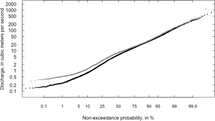
that highest value, the two periods are nearly indistinguishable. This may indicate that there has been little overall change in the upper tail of the distribution, and that one day of the highest flow from Hurricane Irene was simply an outlier rather than an indication of a changing distribution. The fact that the HEFS ensembles do not utilize data from this latter period is troubling, given the rather wide divergence between the ECDFs for the two periods. It will be important for OST used in PA mode to be able to take this widespread and rather dramatic change in the hydrology of the region into account.
REFERENCES
Bronaugh, D., and A. Werner. 2013. zyp: Zhang + Yue-Pilon trends package. R package version 0.10-1. https://CRAN.R-project.org/package=zyp).
Hirsch, R. M., and L. A. De Cicco. 2015. User Guide to Exploration and Graphics for RivEr Trends (EGRET) and dataRetrieval: R Packages for Hydrologic Data. No. 4-A10. Reston, VA: U.S. Geological Survey.
Kendall, M. G. 1975. Rank Correlation Methods, 4th ed. London: Charles Griffin.
Mann, H. B. 1945. Non-parametric tests against trend. Econometrica 13:163–171.
Sen, P. K. 1968. Estimates of the regression coefficient based on Kendall’s tau. Journal of the American Statistical Association 63(324):1379–1389.
Zhang, X., K. D. Harvey, W. D. Hogg, and T. R. Yuzyk. 2001. Trends in Canadian streamflow. Water Resources Research 37(4):987–998.
This page intentionally left blank.


