
2
Description of the Operations Support Tool
OVERVIEW OF THE OPERATIONS SUPPORT TOOL
Surface water supply systems fundamentally involve transformation of precipitation inputs to drinking water by a system of watersheds, reservoirs, conduits, and treatment facilities. The New York City Department of Environmental Protection’s (NYC DEP’s) Operations Support Tool (OST) informs management decisions by formally quantifying flow and quality changes as water moves though the Catskill, Delaware, and Croton systems to New York City. OST can be broadly described as a continuously evolving, state-of-the-art decision support system used by NYC DEP in water supply operations and planning (Porter et al., 2015). Its development was a direct outcome of the Catskill Turbidity Control Study—it was motivated by the need to mitigate fluctuations in source water turbidity in the Catskill system, which have the potential to cause exceedance of the 5 NTU maximum turbidity allowed for diversions from Kensico Reservoir in order to maintain filtration avoidance. In an idealized, simple system focused exclusively on this objective, the Ashokan Reservoir might be primarily managed to store higher-turbidity source water while water quality improves over time due to settling of suspended solids. The accounting of water routing for the New York City water system is not this simple, however, because tradeoffs between multiple objectives such as meeting water demands, controlling floods, and maintaining downstream releases from a large number of reservoirs must be concurrently considered and prioritized.
The OST decision support platform was developed because of the vast number of interdependent decisions that must be made to identify opera-
tional strategies that consider and appropriately balance multiple objectives at any point in time and in response to a wide range of possible future conditions. Although OST is not needed for operational responsiveness in some cases, it is intended to simulate decisions that closely approximate the decisions that a knowledgeable operator would make after considering and processing all of the available data, constraints, and possible operational controls. Manual completion of this task for the complex NYC DEP water system may not allow for a complete evaluation of operational options; therefore, it is done by utilizing water quantity and water quality models that provide simulation of flows, reservoir levels, and water quality under a range of possible conditions for a future time period. OST is a flexible and modular platform—it accounts for water routing and provides the probability of predicted future operational conditions based on a wide range of near-real-time (meteorologic, hydrologic, and water quality) data, several (deterministic and stochastic) modeled relationships, regulatory constraints, and operational insight.
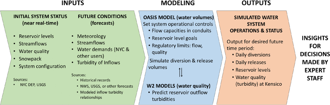
Figure 2-1 summarizes the conceptual framework of OST (and is a more detailed version of Figure 1-6). Shown in green, near-real-time data describe the current status of the water system, providing “situational awareness” for NYC DEP as well as the initial system conditions for model forecasts. Models (in blue) for water quantity (OASIS) and water quality (CE-QUAL-W2) combine forecasts of future water inputs (precipitation and streamflow) and system attributes to simulate future water flows and reservoir storage conditions. The model outputs (in red), such as diversions, releases, reservoir levels, and water quality conditions, are used for decision making, communicating, and understanding various metrics of system performance.
As previously noted, the origin of OST was the Catskill Turbidity Control Study conducted as part of NYC DEP’s long-term Watershed Protection Program (see Chapter 3), which allows the City to avoid filtration of the Catskill/Delaware water supply (Weiss et al., 2013). Over many years, the Catskill Turbidity Control Study assessed various operational and structural options to minimize turbidity emanating from the Catskill system, including the development of a combined water quantity–water quality model that could improve reservoir operations. From a water quality regulatory perspective, the ultimate operational goal is to not exceed the Surface Water Treatment Rule’s mandated maximum allowable turbidity of 5 NTU for water leaving the Kensico Reservoir prior to ultraviolet (UV) disinfection. Controlling the turbidity of water entering the Catskill Aqueduct is one important aspect of meeting the Kensico turbidity objective.
This discussion of OST does not focus on any one particular release of this tool but rather on the concept and on areas of possible future development. It is important to recognize that OST does not dictate operations of
NWS = National Weather Service; USGS = U.S. Geological Survey.
any aspect of the water supply system. Operational decisions are always made by the staff of the NYC DEP. The role of OST is to inform water system managers of the potential consequences of any particular set of decisions and to provide a basis for comparing multiple operational options.
OST components include real-time, historical, and predicted data that describe water quantity and water quality attributes, models of water quantity and quality, and reporting of model outputs expressed as metrics of system performance (as shown in Figure 2-1). These metrics include measures of (1) reservoir storage at various times in the future (from days to weeks to months), (2) departures from target storage levels, (3) maximum turbidity levels at key locations in the system, and (4) degree of achievement of various goals for the system (such as targets for releases to downstream river reaches).
By using multiple predictions of future hydrologic conditions, OST provides estimates of conditional probability distributions of the metrics of system performance. As described in Box 2-1, conditional probability distributions take into account the current status of a system in describing the likelihood of a future condition (e.g., streamflow), in contrast to marginal probability distributions that are based only on the historical record and are independent of current status. Effective operation of any water supply system depends on a balancing of the risk of certain undesirable outcomes such as failure to deliver sufficient water to customers, violation of a water quality standard, and reservoir releases that have negative impacts on downstream parties (either for their water supply or for other uses such as recreation). OST is designed to provide frequently updated estimates of the probabilities of many of these outcomes and to evaluate how near-term changes in system operations can influence these probabilities.
OST Versus Other Methods for Operational Decision Making
OST departs from traditional methods of analysis for water supply operational decision making. The most common historical approach in many agencies, including the NYC DEP, has been to make operational decisions based on a static rule curve. This curve, which plots a target reservoir storage level as a function of the day of the year, represents the desired storage level in a given reservoir. That target is designed to balance the risk of water supply shortage against the risk of downstream flooding. The former concern motivates the operators to attempt to maintain a high level of storage prior to the beginning of a possible dry period while the latter concern motivates the operators to attempt to maintain a low level of storage so that the reservoir has the capacity to accept flood waters, for example when snowmelt occurs. The rule curve is established, typically by simulations of past hydrology and expected water deliveries, to maintain a
balance between these two measures of risk. The rule-curve approach often involves multiple curves that are used as indicators of the magnitude of the risk, and management actions are based on the reservoir storage being in some “zone” (which lies between successive levels of these rule curves). For example, if a certain storage value is required on April 1, the set of rule curves dictates a set of management actions that should be undertaken. These actions can include greater use of an alternative but more costly source of water, curtailing downstream releases, or imposing water-use restrictions on customers.
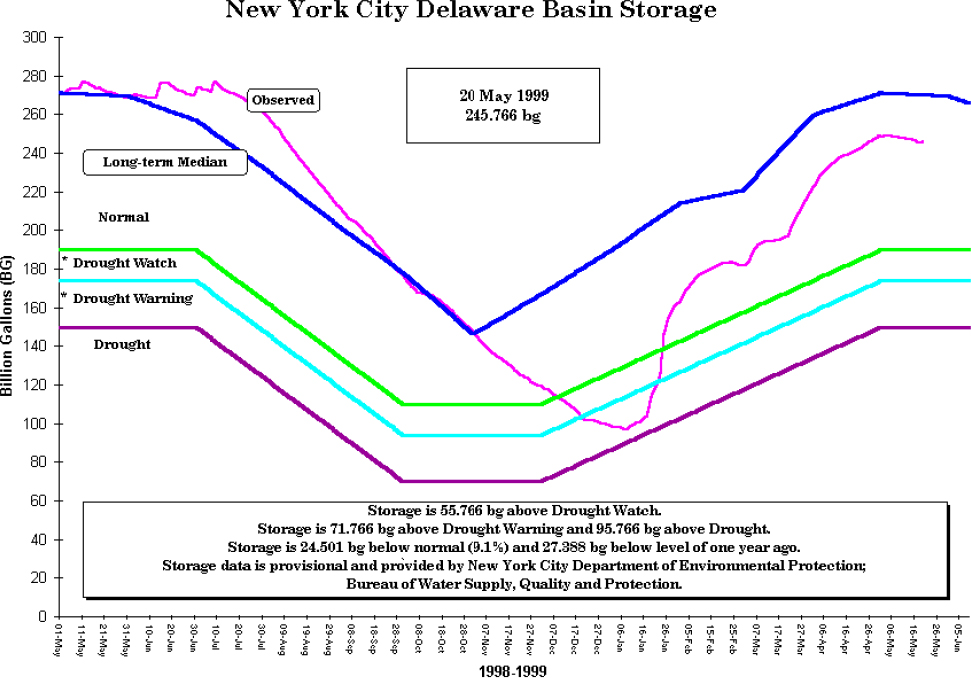
An example of the rule-curve approach is shown in Figure 2-2, which covers a time period that includes one of the most severe droughts that has taken place in the New York City water supply system over the past 50 years. It took place before NYC DEP had adopted an ensemble forecasting-based approach to water supply management. What Figure 2-2 shows is that storage in the Delaware Basin portion of the system was at, or slightly above, its long-term median level from May through October 1998, but around November 1998 storage began to fall below its historic median levels. By December 1998 storage had fallen to a level that triggered a “drought watch.” Within the month of December the system entered the “drought warning” zone. Conditions then improved in January and the system emerged from the drought warning and drought watch zones into the “normal” zone through the rest of the winter and spring.
Assigning management actions to certain storage zones had been the traditional approach to reservoir management for the NYC water supply. The rule-curve approach does take advantage of knowing the present state of water storage in the system. However, the approach (1) does not take advantage of knowledge of overall hydrologic conditions (characterized by streamflow, soil moisture, and snowpack) in the watershed, only the reservoir storage; (2) does not take advantage of weather forecast information; (3) cannot capture the range of conditions that exist across the multiple reservoirs and watersheds in the water supply system (they are generally designed as if the only source of water was a single reservoir); and (4) does not quantify the level of risk associated with the current storage situation (e.g., we may be below the desired storage level for the time of year, but we have no knowledge of whether the future risk of shortage is low or high).
Use of OST provides (1) quantification of the current conditional probability of water supply shortages over the coming year and (2) quantification of how near-term (days to weeks) management actions might change those probabilities. This type of information helps managers communicate to higher-level decision makers and the public the severity of the risks and how certain actions that may be costly or have some negative consequences on the public or natural resources might help to reduce those risks. Decisions that incorporate these types of additional information can
be expected to provide a better basis for decision making about system operations.
The other common approach to analysis for water supply operations is to use a single future scenario (the most likely or mean forecast). In this approach, one takes the “best estimate” of future atmospheric inputs (primarily precipitation and temperature forecasts) and uses those as inputs to a watershed hydrologic model to create a single time series of inflows to the reservoirs. Then, using some operational assumptions (typically a rule curve), managers estimate a most likely or mean state of the system at some target date in the future. This type of output turns out not to be very useful to the managers. They know that beyond a few days, weather forecasts, and hence hydrologic forecasts, have very little accuracy and thus they know that actual outcomes can be very different from these most likely or mean forecasts. What they would really like to know is the probability of certain types of “bad outcomes” occurring over some multimonth
operational time horizon. Examples of bad outcomes would be (1) needing to call upon customers to temporarily curtail their water use, (2) delivering water to customers that is less than the quantity that they demand (resulting in service interruptions), (3) releasing less than the target amount of water to some downstream reach (resulting in fish kills, or impairment of recreational opportunities), or (4) violating water quality goals in the reservoirs or in the water delivered (resulting in the need to use large amounts of treatment chemicals or the need to make long-term investments in treatment works). The objective of the type of forecasting being employed in OST is to be able, at any point in time, to estimate the probability of bad outcomes such as the ones mentioned here, and furthermore, to be able to assess how changes in system management in the near term might change those probabilities.
The OST approach is a significant step forward from NYC DEP’s past methods of reservoir operations because it places the focus of management
information on computing the conditional probability distributions of various outcome measures at various time horizons. OST allows the NYC DEP to determine the impact that specific near-term management actions will have on these conditional probability distributions. In this way, they can evaluate the sensitivity of those risks to the management actions they take in the near term. OST is a flexible tool that allows these risk estimates to be recalculated frequently (e.g., weekly or even daily) based on changing storage levels, the changing state of hydrologic state variables, and changing weather forecast information. Because the set of management decisions that are made is complex (releases and diversions of water at many locations in the system), the OST simulations need to make use of operating rules to approximate the decisions that managers would likely make at various times in the future (weeks to months ahead). Importantly,
however, there is no requirement that managers actually follow the simulated actions (e.g., diversions and releases) when the time arrives.
OST DATA FLOW AND OUTPUTS
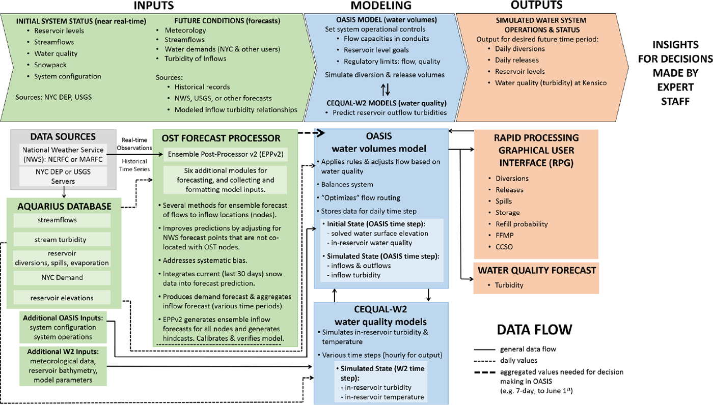
As shown in Figure 2-1, OST uses water quantity and water quality models to combine forecasts of watershed tributary flows and water demands with various constraints and goals (such as physical/hydraulic attributes, operating rules, and weighting factors) to determine (1) daily diversions (flow through aqueducts), (2) daily releases (flows to rivers downstream of reservoirs), and (3) water quality (presently turbidity and temperature) within the New York City water system. To do this, OST is first initialized with input data that describe the initial status of the system, including the current volume of storage in each of the reservoirs, streamflows in relevant river reaches, and critical water quality (i.e., turbidity) conditions at various points. A number of internal and external data sources are used to provide this information in near real time. These data flow through a forecast processor to the OASIS and CE-QUAL-W2 models, which form the quantitative backbone and modeling framework of OST. This flow of information is shown in detail in Figure 2-3, which is an elaboration of Figure 2-1.
Figure 2-3 is exhaustive in the sense that all major data flows through OST are represented. It was created to convey the complexity of the tool to the reader. However, this chapter emphasizes those parts of OST that the Committee deemed were either controversial or in need of improvement; hence, not all parts of Figure 2-3 are discussed equally. The chapter focuses on the OASIS and CE-QUAL-W2 models as well as the ensemble streamflow forecasts and turbidity-flow relationships that are inputs to OST.
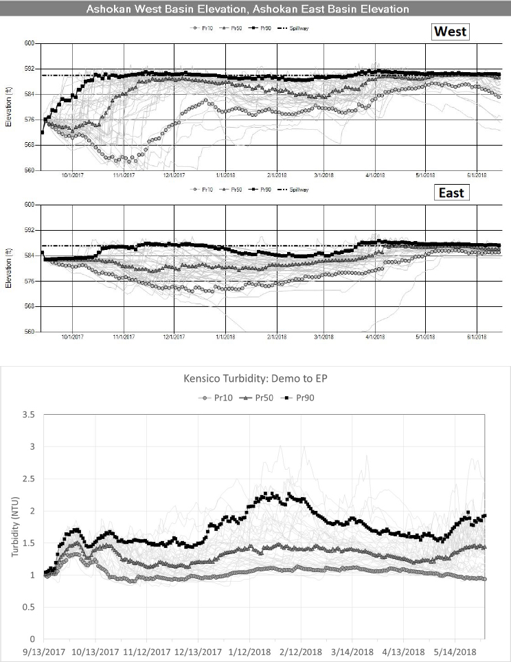
The typical outputs from an OST run are one or many time-series simulations of (1) future reservoir diversions and releases, (2) future reservoir storage as described by basin elevation, and (3) future water quality conditions such as turbidity in Kensico. Figure 2-4 gives two examples of such output resulting from an ensemble of 48 different possible future streamflow scenarios, all starting on the same date in September 2017. Each line, or trace, in Figure 2-4 shows simulated conditions resulting from one time series of future stream flows. Managers can use the results for the ensemble of individual simulations to develop conditional probabilities for specific conditions or events to occur, providing a basis for assessing system reliability and making day-to-day decisions about system operation. For example, the lower panel of Figure 2-4 shows that there is a 90 percent probability that Kensico turbidity will not exceed approximately 2.2 NTU over a future nine-month period (the boxed line is the 90th percentile over all 48 possible traces, such that 90 percent of all traces lie below that line).
NYC DEP uses software called a Rapid Processing Graphical User Interface (GUI) to extract the OST output for the metrics of interest to NYC DEP. The GUI enables the user to access input and output files, manage simulation executions, and enter modeling assumptions (Porter et al., 2015). Since OST archives all operational data, including reservoir levels, water flows, water quality, and environmental information, the GUI also provides a means to generate specific and recurring reports and documentation derived from these data. The reports are customizable for internal and external users, to include production of tables and plots, and the data can be further exported for other data processing programs. Especially beneficial is the ability to develop outputs for use in the evaluation of numerous operating assumptions and their impact on near-term and long-term operations. An example is an evaluation of the implications of modifying existing operating rules (e.g., meet water supply demand and water quality needs while balancing the desire to refill all system reservoirs by June 1 of each year). Another example is to explore how certain assumptions or scenarios will affect the water supply, such as exploring the impacts of an exceptionally wet or dry year or the impacts due to temporary isolation of a part of the system because of scheduled or unscheduled maintenance (Porter et al., 2015). NYC DEP has, for many years, been in the forefront of water supply agencies in evaluating conditional probabilities, utilizing models and ensemble forecasts to support operational decisions. The models in OST are also used to simulate longer-term future system scenarios, such as scheduled changes in system infrastructure or long-term impacts of climate change, for planning purposes.
MODELS USED IN OST
OST uses water quantity and water quality models to combine forecasts of watershed tributary flows and water demands with various constraints and goals (e.g., physical/hydraulic attributes, operating rules, and weighting factors) to determine daily diversions (flow through aqueducts) and releases (flows to rivers downstream of reservoirs) and their associated water quality (mainly turbidity and temperature) for the New York City water system (Figure 2-1). The backbone of OST is the systemwide water quantity accounting model OASIS (Operational Analysis and Simulation of Integrated Systems; HydroLogics, Inc., 2009), which can interact with the CE-QUAL-W2 reservoir water quality and hydrodynamic models. The OASIS model serves as the foundational tool for simulating the inflows (tributaries and diversions) and outflows (releases and diversions), and thus storage levels, for each of the reservoirs in the Delaware, Catskill, and Croton systems. CE-QUAL-W2 (Cole and Wells, 2002, 2015) two-dimensional hydrodynamic and water quality models, colloquially
called W2, have been developed to model turbidity for Schoharie Reservoir, the West and East basins of Ashokan Reservoir, Rondout Reservoir, and Kensico Reservoir. The development of the W2 models for reservoir water quality provides the opportunity for NYC DEP to simulate the impact of future meteorological and climate conditions on the quality of water diverted from the Kensico Reservoir. This water becomes the influent to the Catskill–Delaware Ultraviolet Disinfection Facility and then is the most significant, or only (when the Croton system is not operating), source of potable water for New York City. As part of an unfiltered surface water system, Kensico Reservoir water quality is controlled by natural watershed processes, engineered water storage and transport facilities, and limited use of alum addition upstream of the reservoir.
The independent W2 models can be linked to the OASIS model to provide water quality information inputs to OASIS. OASIS and W2 can be executed sequentially such that for each simulation day, OASIS provides water quantity (flow) information for W2, and W2 then provides water quality information for use in the next OASIS simulation day (NYC DEP, 2010). The linked water quantity and water quality models are thus able to simulate the interactions between water quality and reservoir release and diversion decisions.
The OASIS model does not simulate water quality; however, water quality affects OASIS model results through coded operating rules that are based on water quality. Currently, turbidity is the only water quality parameter that affects the OASIS model. Turbidity impacts are considered based on both the level of turbidity (as quantified by NTU) and the loading of turbidity as quantified by the product of flow rate and turbidity. As described in more detail in the following section, the OASIS operating rules related to water quality are based on institutional knowledge and various regulations. For example, the level of turbidity in the Schoharie Reservoir affects allowable transfers to Ashokan West Basin via the Shandaken Tunnel and Upper Esopus Creek. Along with flow and elevation factors, turbidity impacts the transfer of Ashokan Reservoir water between the West and East basins, the diversion of Ashokan water to the Catskill Aqueduct, and the release of water to the Lower Esopus Creek through the Ashokan Release Channel (as described in the Interim Release Protocol). Turbidity load in the Catskill Aqueduct affects the use of the Shaft 4 interconnection between the Delaware and Catskill aqueducts, Catskill Aqueduct flow, and the decision to apply alum at the Catalum facility ahead of the Kensico Reservoir. In all of the previous examples, water quality requirements can affect the output of the OASIS model. Similarly, the W2 reservoir models are affected by diversion and release decisions. The W2 model of Schoharie Reservoir provides input via the Upper Esopus Creek to the West Basin of Ashokan Reservoir, which then provides input to Ashokan’s East Basin
via the dividing weir spillway and gates. The outputs from the West and East Basin Ashokan W2 models, and potentially the Rondout W2 model, are used to provide water quality simulation for diversions to the Catskill Aqueduct, which ultimately flows into Kensico Reservoir, and thus are inputs to the Kensico W2 model. If used, alum addition at the Catalum facility also impacts the Kensico W2 model.
The OASIS model can be run with or without the W2 models. Computation time is significantly increased when the W2 model is integrated into the OASIS run, increasing from about 2.5 minutes to simulate an ensemble of 48 one-year-duration inflow scenarios for OASIS alone to 20 minutes if only several weeks of W2 simulations are included. If the W2 models are not used, recent and historical turbidity data, as well as projected tributary flows, are used for assigning turbidity levels to flows in the Delaware and Catskill aqueducts. The W2 models operate on much shorter time steps than the OASIS model and make use of tributary inflow and water quality, as well as meteorological conditions, to model reservoir water quality.
More detailed descriptions of the OASIS and W2 models in OST, the uses of the models, and model data inputs are provided in the following section.
OASIS Water Quantity System Model
The OASIS model is a proprietary model developed and maintained by Hydrologics, Inc. (2009). OASIS uses a linear programming approach to determine daily volumes for reservoir releases and diversions based on physical constraints and user-defined operating goals. These constraints and goals are how the user tells OASIS what to do, without having to specify the details about how to do it. The way that OASIS solves for routing decisions using its linear programming formulation is unique, and somewhat of a departure from the significant research literature on optimal reservoir operations. As described in the OASIS User Manual (HydroLogics, Inc., 2009):
Some modelers in the water resources field have used linear programming to optimize the operation of a system over a period of record with a single optimization. OASIS works very differently. OASIS simulates a period of record by optimizing the operations for a single time step, then going on to the next time step. Thus a 60-year record with a monthly time step would result in 720 separate optimizations. In the other modeling approach, the model has “perfect future knowledge,” where the inflows and demands are known for the entire record at the start of the run. This allows the system to respond, for example, to a flood a year before it occurs. OASIS’s running from time step to time step is much more realistic since it is more like how the operators, who are not blessed with perfect future knowledge, control the system.
As described by NYC DEP (2010), the multiple objectives of the NYC DEP water supply system include reliably meeting the water demands of New York City and outside communities; maximizing the quality of water leaving Kensico Reservoir, currently based on turbidity; maximizing environmental benefits for users and the ecosystem downstream of reservoirs; and meeting flood mitigation and recreation objectives, all while considering economic impacts related to the costs of pumping and treatment. These objectives have guided the formulation and configuration of the OASIS model, including the specification of key parameters that affect routing decisions, as described in the following section.
OASIS simulates the physical attributes of a water supply system as a system of nodes (reservoirs, demand locations, junctions) and arcs (aqueducts, streams, usually between nodes). Based on user-supplied time series of tributary inflows and water demands; physical system attributes (storage vs. elevation for a reservoir, head-discharge relations, spillway capacities, current system status); and specified operating rules, an OASIS model run or solution provides a forecast of daily volumes for diversions and releases along with associated changes in storage for all reservoirs. Forecast periods range from weeks to years, with a one-year duration typical for use of OST in “position-analysis (PA)” mode. (Options for the future tributary inflow time series to be used and for the different modes or approaches for using the OST are described later in this chapter.) The output of an OASIS model run for a single time series of inflows is known as a trace. A set of traces for which the only change between runs is the series of inflows for the same future time period is known as an ensemble.
The OASIS model linear program solver seeks a solution that maximizes the overall value or score for the system for that day, subject to water mass balance conditions, physical/hydraulic attributes, and a wide array of user-defined operating rules, commonly described by coded operating constraints and operating goals. The objective function of the linear program can be written as:
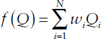
where Qi is a decision variable (daily flow volume for a diversion, release, or delivery, or a storage volume for the ith variable), wi is a weighting factor for that variable, and N is the total number of variables (volumes).
Operating constraints are conditions that must be met in order for a feasible solution to be realized (e.g., minimum reservoir storage, Kensico diversion turbidity limit cannot exceed 5 NTU, or conservation of water mass at a node). To provide maximum modeling flexibility and minimize infeasible outcomes, the NYC DEP OASIS model includes relatively few constraints. In contrast, operating goals are targets to be achieved (e.g.,
reaching 100 percent storage capacity in the reservoirs as of June 1, certain releases, or balancing storage) but do not have to be reached in order for a feasible solution to be found. Each operating goal has an applied “weight” to influence model outcomes by establishing the relative priority of multiple goals. For example, meeting the NYC water demand is the highest priority, so diversions to meet that demand (e.g., from Kensico and/or the Croton supply) are highly weighted or valued compared to an above-minimum required release from a reservoir that increases ecosystem services. Another example is assigning a higher weight or value to lower-turbidity water as compared to higher-turbidity water in order to meet water quality objectives. Weights are discussed in more detail later in this chapter.
The various operating rules that impact reservoir diversions and releases are captured in a series of Operations Control Language (OCL) modules. Operating rules (both constraints and goals) include user-defined OCL constants that quantify aspects of the variables considered by an operating rule. Table 2-1 lists a few examples of OCL constants used in operating rules for OST. The value of an OCL constant is based on a range of factors, including system hydraulics (e.g., hydraulic capacity of a tunnel section), regulatory constraints (as explained in the following section), water quality (e.g., turbidity trigger to invoke goal to decrease diversion from Ashokan Reservoir to the Catskill Aqueduct), and practical operational limits (e.g., frequent insertion and removal of stop shutters in the Catskill Aqueduct should be avoided). The OCL modules capture the range and complexity of the large number of factors that affect operation of the NYC DEP water system.
TABLE 2-1 Examples of OCL Constants
| OCL Constant Name | Description; default value |
|---|---|
| [CatAq_min_SS] | Minimum diversion from Ashokan when stop-shutters are in; 25 MGD |
| [TrigTurbVal_CatAq] | Catskill Aq. turbidity level at which reduce diversion; 8 NTU |
| [CatAq_StopShutter_Trig] | Catskill Aq. turbidity level at which stop-shutters are in; 18 NTU |
| [Alum_Trigger] | Catskill Aq. turbidity load trigger for alum application; 5000 MGD∙NTU |
| [Use_Shaft4] | Use shaft 4 inter-connection; 0 (don’t use) |
| [CatAq_rem_StopShut] | Five-day average Catskill Aq. turbidity at which remove stop-shutters; 8 NTU |
| [Ash_DivWeir_Max UnseatedHead] | Maximum head differential (East > West); 20 ft. |
SOURCE: Courtesy of NYC DEP.
How OASIS Is Run
The OASIS model is initialized to either the present state (position) of the NYC water supply system for “position analysis” purposes (position analysis mode) or to an alternative set of initial conditions for longer-term planning/evaluation simulations (simulation mode). (The differences between position-analysis mode and simulation mode are discussed in greater detail in a later section.) Initial condition variables include the current volume of storage in each of the system reservoirs, the status of “state variables1” in the hydrologic model, the flows of water in downstream river reaches that are influenced by releases from the system reservoirs, measures of critical water quality conditions (typically turbidity at various points in the system), and any constraints on delivery of water through specific tunnels or aqueducts (e.g., due to system maintenance service outages).
The OASIS simulation includes representations of water budget accounting at a set of nodes in the system, all of which are based on principles of conservation of water mass. Hence, at any given node, change in storage over any time step equals all inflows minus all outflows. For a reservoir node, changes in storage will increase or decrease the water level in the reservoir. For a node without storage, such as the intersection of two aqueducts or the point of withdrawal along an aqueduct, the sum of the inflows equals the sum of the outflows. Inflows can include (1) uncontrolled river inflows, (2) diffuse groundwater inflows, (3) delivery from an aqueduct or controlled release from an upstream reservoir, and (4) direct precipitation on a reservoir. Possible node outflows are (1) the flows to downstream river segments (which may be a combination of releases and spills), (2) diversions to an aqueduct, (3) evaporation from the reservoir, and (4) water demands for New York City and other supplied communities. The simulation includes rules for routing water via links between system nodes (arcs), as influenced by the hydraulic characteristics of the link (a channel or aqueduct segment) as well as the time of travel between nodes.
The OASIS simulation can also include mass balance-based calculations for the concentration of a water quality constituent at a node. The model addresses conservative (nonreactive) constituents only, although a constituent can be increased or decreased at a node by applying boundary conditions (fractional or additive). For example, the node mass balance for turbidity is based on inputs from upstream segments (arc concentrations are based on the upstream node concentration), dilution by perfect mixing in a reservoir, and outflows (diversions and releases). Settling and deposition in a reservoir, or scour of particles from reservoir sediments into the
___________________
1 State variables are model representations of the status of water storage in soil, groundwater, and snowpack. They may be based on direct measurements or may be inferred based on watershed model simulations up to the present.
reservoir, can be simulated using a boundary condition for the reservoir node. Some of the operating rules in OASIS include impacts on diversion and release flows based on either turbidity levels or turbidity loads (turbidity times flow). Natural streamflow turbidities are simulated based on streamflow and seasonal data. The W2 water quality models can be used to simulate in-reservoir turbidity and thus the turbidity of diversions and releases. Initial-condition turbidities are based on measured values in the water system. When W2 is not utilized, turbidity is not modeled within OASIS. However, the possible occurrence of high-turbidity inputs to the Catskill Aqueduct associated with high streamflow is reflected in OASIS operating rules that impact diversions based on streamflow forecasts only.
The OASIS model for the NYC DEP water system is integrated with an OASIS model for the overall Delaware River Basin (DRB) because downstream Delaware River flow levels and other factors can constrain releases from NYC DEP reservoirs in the Delaware watershed (Cannonsville, Pepacton, and Neversink). These aspects are described in the Flexible Flow Management Program for the Delaware River Basin, of which NYC DEP is part (USGS, ORDM, 2017).
Diversions and releases from the Schoharie and Ashokan reservoirs of the Catskill system are affected by various New York State laws and regulations, including the Shandaken Tunnel State Pollutant Discharge Elimination System (SPDES) permit; various New York Codes, Rules, and Regulations regarding reservoir releases; the Interim Release Protocol (IRP) for Ashokan Reservoir; and the Catalum SPDES permit (see Chapter 1). An example of an OASIS operating rule affected by a regulation is code that does not allow a diversion via the Shandaken Tunnel to the Upper Esopus Creek if the Schoharie Reservoir withdrawal turbidity exceeds 100 NTU (subject to some exceptions). Such a situation could be caused by a known initial condition at the start of a model run, by a future predicted high turbidity based on CE-QUAL-W2 model results, or by expected impacts of high Schoharie Creek flow on reservoir turbidity.
Weights and Penalties Within OASIS
The linear program solver in OASIS determines daily values (water volumes) for each decision variable (diversion, release, and demand flows; storage volumes) such that the “score” for the day is maximized. Each decision variable has a user-assigned numerical weight that is multiplied by the value of the decision variable when computing the contribution of that variable to the overall score of the system. The relative values of the weights indicate the relative priority of the water volume represented by that variable. Weights are assigned to demand and reservoir node variables as well as to arc variables. For example, demands for NYC and for other communities are assigned
a weight to prioritize meeting demand (the score for the system would be greatly decreased if the value of the demand variable was decreased below a target value). Other node variables with high priority include the lower, or “dead,” storage in reservoirs, which prioritizes not using that storage volume. In contrast, storage above the dead storage zone is assigned a weight such that it is utilized first. Examples of relative weights for diversion/release flows (arc variables) include weights to prioritize minimum release flows below dams and weights to very much discourage spills from Rondout Reservoir (because the water quality is usually very good).
Relative priorities for different water volumes (decision variables) are also impacted by assigning penalties based on the degree to which desired operating goals are not met or based on water quality constraints. For example, a target might be to have equal relative storage between several reservoirs; an OCL target command and associated penalty can be used to favor use of water from one reservoir over another in order to achieve the balancing goal. A water quality-based example would be to penalize and/or constrain the diversion of Ashokan water to the Catskill Aqueduct if the Ashokan turbidity exceeds a certain set point (as defined, for example, by an OCL Constant, see Table 2-1).
The initial assignment of values for weights and penalties was undertaken by NYC DEP and contractors during development of the OASIS model and OST overall. Presumably, the values were assigned to calibrate/validate the model to yield appropriate performance of the system as would occur based on decisions made by knowledgeable human operators, hence creating the “expert system” aspect of OASIS. The relative values of the weights and penalties, as well as the coding of operating rules, reflect the relative priorities of different water volumes to NYC DEP. The Committee feels that exploration and communication of the sensitivity of simulated operational decisions to the magnitude of the weights and penalties should be undertaken. This consideration may be especially important in the use of OST as part of the Environmental Impact Assessment for the Catalum SPDES permit modification (see Chapter 4).
CE-QUAL-W2 Models
CE-QUAL-W2 (W2) is a public domain, two-dimensional (vertical and longitudinal; lateral homogeneity assumed) model for hydrodynamics (water velocity, water level) and water quality that is appropriate for water systems with high length-to-width ratios such as rivers and many reservoirs (Cole and Wells, 2002, 2015). The bathymetry of a water body is described by multiple connected segments, each with multiple layers of varying width (and depth as desired). Water inflows (tributaries, aqueducts) and outflows (to aqueducts, spillways, downstream rivers) are allocated to specific
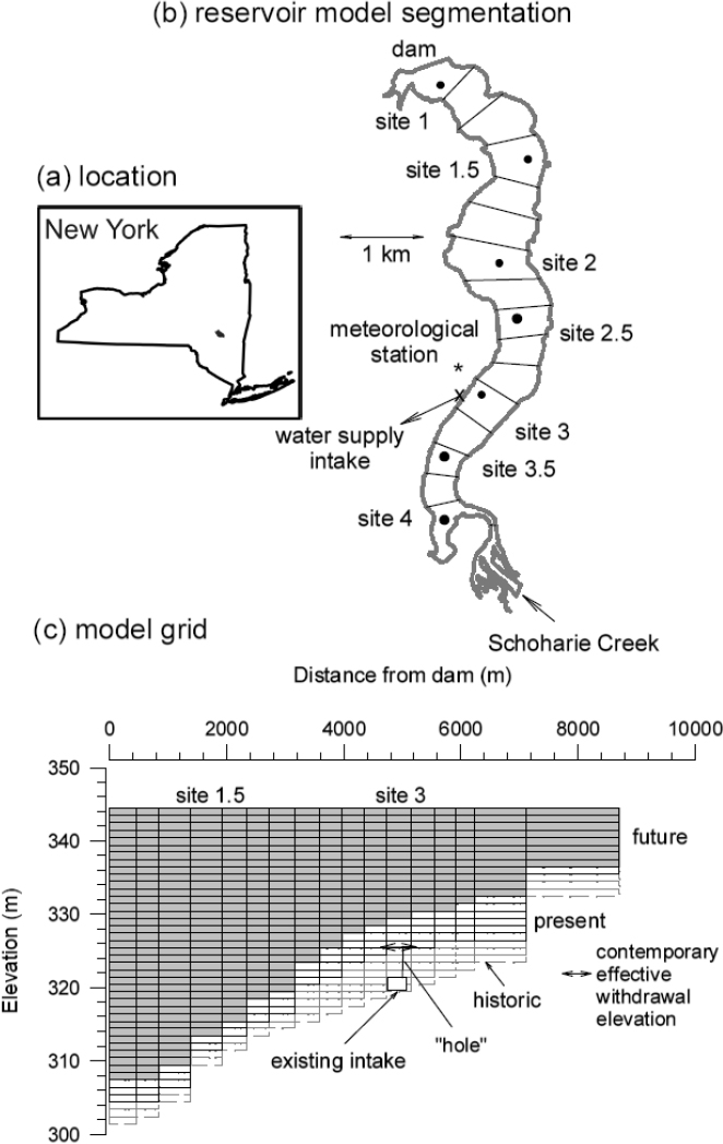
segments. Each layer in a segment is a well-mixed element that interacts with adjacent elements and boundaries (air above, sediment below). An example of reservoir segments and vertical layers is shown in Figure 2-5 for the Schoharie Reservoir. Within W2, the transport of fluid momentum, mass, and energy (temperature) between elements is determined based on appropriate conservation equations. A variety of water quality parameters can potentially be modeled in W2 based on within-element transformations (reactions) as well as transport between elements and to/from boundaries. However, in the current application only turbidity is modeled.
The W2 model output describes the temporal evolution of spatially distributed water velocities and water quality due to the impacts of inputs, outflows, and within-element processes on the initial waterbody conditions. Required data include temporal series of inflows with associated water quality, outflows, and meteorological conditions (precipitation on the reservoir; air properties such as temperature, relative humidity, wind speed, and direction; solar radiation; and cloud cover).
Over 20 years ago, the NYC DEP began developing W2 models for its reservoirs. Until a few years ago, NYC DEP contracted with the Upstate Freshwater Institute (UFI) to develop, calibrate, and validate hydrodynamic and water quality models for many of its reservoirs. OST currently includes W2 models developed for the Kensico, Ashokan (West and East basins), Schoharie, and Rondout reservoirs, with plans to include models for Cannonsville, Neversink, and Pepacton reservoirs (W2 models for these reservoirs have been developed but are currently used for other purposes outside of OST). Because of the filtration avoidance determination (FAD) and the critical goal of meeting turbidity requirements for water withdrawn from the Kensico Reservoir, the focus of the water quality modeling to date within OST has been on turbidity. Potential future development will include modeling of natural organic matter, probably as described by dissolved organic carbon (DOC) and disinfection by-product (DBP) precursors. Calibrating and validating W2 models typically involves comparing predictions and measurements of spatial and temporal series of reservoir water surface elevation, water temperature, and often a nearly conservative water quality parameter such as total dissolved solids (as assessed by specific conductivity). Ideally, the calibration and validation periods should include the full range of historical flow and water quality conditions for the water body.
The W2 modeling platform includes a number of specific water quality parameters as well as options for generic water quality parameters. However, turbidity is not explicitly included in the standard W2 software. Turbidity is a challenging parameter to model because it is an indirect measure of particulate matter in water that depends on both the amount and the characteristics (size, shape, material) of suspended particles. The W2 software does include a direct measure of particulate matter known as total sus-
pended solids (TSS), expressed as mass of solids per unit volume of water. In general, turbidity is positively correlated with TSS but the correlation can be very site specific, complicated, and uncertain. In addition, measurement of TSS is more difficult and expensive than measurement of turbidity. Also, turbidity is the regulated water quality parameter, so it is best to model it directly. The W2 model includes several optional “generic” water quality constituents that can have associated characteristics that affect their fate in the water column; for example, for turbidity, a settling velocity can be assigned, resulting in vertical transport to the reservoir bottom. The UFI W2 model developers decided to utilize the generic constituent options within the W2 software to enable modeling of the spatial and temporal variations of turbidity in the NYC DEP water system reservoirs.
Schoharie Reservoir
UFI developed a W2 model for the 19.6-billion-gallon (BG) Schoharie Reservoir, the most upland reservoir in the Catskill system. Gelda and Effler (2007) described the initial basis for developing the turbidity modeling component, which included use of the attenuation of 660 nanometer (nm)wavelength light as a directly correlated surrogate for turbidity. The turbidity of water is significantly influenced by the size of suspended particles. In natural systems, particles are removed from water by settling to the bottom of the water body. The rate of particle settling is strongly influenced by particle size, particle density, and water temperature. Naturally occurring particles typically have a broad particle size distribution; therefore, the rate of particle settling, and thus removal of turbidity, is not uniform across the particle size distribution. Gelda and Effler (2007) investigated the use of one, two, and three separate particle fractions to represent turbidity, with each component assigned a separate settling velocity. The authors concluded that multiple particle fractions were needed to model turbidity, with the distribution of fractions and associated settling velocities determined by analysis of particle size distributions and model calibration. The three-component model allocated 20, 45, and 35 percent of the particles into fractions with respective settling velocities of 0.01, 2.5, and 5 m/day, corresponding to particle sizes of 0.42, 6.59, and 9.31 micrometers (µm). Particles in reservoir inflows, dominated by the Schoharie Creek (75 percent), were allocated into the fractions, and total inflow turbidity was correlated with tributary flow rate. Model simulations of temporal turbidity values were in excellent agreement with measurements for three water depths at two different sites for a six-month period in 2003 (Gelda and Effler, 2007).
Current use of the Schoharie Reservoir W2 model provides predictions of the turbidity of water diversions to the Ashokan Reservoir via the Shandaken Tunnel and Upper Esopus Creek.
Ashokan Reservoir
The 127.9 BG Ashokan Reservoir in the Catskill system has hydraulically distinct West and East basins that are separated by a dividing weir. The vast majority of flow enters the Ashokan via the Upper Esopus Creek to the West Basin, and almost all inflow to the East Basin is from the West Basin. The West Basin serves as a sedimentation basin for turbidity-causing particles, providing an opportunity for the East Basin to have lower-turbidity water. Diversions to the Catskill Aqueduct are typically from the East Basin, although withdrawals can be made from either basin. Release of water to the Lower Esopus Creek below the reservoir is typically made via the Ashokan Release Channel, although spillway discharges can also occur.
Gelda et al. (2009) described the development of the W2 model for Ashokan Reservoir, which includes three separate particle components for modeling turbidity within each basin based on inflow turbidity loading, reservoir hydrodynamics, water diversions and releases, and particle settling. The W2 hydrodynamic model was calibrated using 13 years of data. Turbidity was modeled directly as the state variable with contributions from three size classes (1, 3.1, and 8.1 µm), each with a settling velocity (0.075, 0.75, and 5.0 m/day at 18°C) and fraction of the total inflow turbidity from Esopus Creek (10, 65, and 25 percent for Q < 40 m3/s, and 10, 45, and 45 percent for Q > 40 m3/s, reflecting more larger-particle contribution at higher inflow). The assignment of size, settling velocity, and fraction was based on extensive analysis of thousands of individual particles. Modeling showed that three size classes provided better simulation than one or two size classes but that greater than three size classes did not provide significant improvement in the simulation accuracy. The turbidity model was calibrated based on extensive monitoring data from 2006 and validated for two other time periods. Normalized root mean squared errors for the peak turbidity of water diversions to the Catskill Aqueduct during multiple events in 2005 and 2006 were less than 25 percent. Simulation of the duration, peaks, and spatial distribution of in-reservoir turbidity was generally good.
The Ashokan W2 model allows for prediction of turbidity in water diversions to the Catskill Aqueduct and in water releases to the Ashokan Release Channel. Such predictions are important aspects of making operational decisions regarding Ashokan for drinking water supply as well as for ecosystem services, flood mitigation, and turbidity control in the Lower Esopus Creek.
Kensico Reservoir
The 31.4-BG Kensico Reservoir receives inflows from both the Catskill and Delaware aqueducts. A UFI-developed W2 model for the Kensico Reservoir has been described by Gelda et al. (2012). The turbidity for both
the Catskill and Delaware withdrawals from Kensico are obviously very important with respect to meeting allowable maximum turbidity levels for the potable water supply. Thus predictions of Kensico turbidity are important with respect to use of OST to support diversion and release decisions.
An important and challenging unique feature of the Kensico W2 model is the need to capture the impact of alum addition at the Catalum facility on the Catskill Aqueduct turbidity as it enters Kensico. The model developers successfully incorporated the impacts of alum addition and also included two separate state variables to model the spatial deposition of precipitated aluminum hydroxide and associated coagulated clay particles (referred to as “alum sludge” in NYC DEP documents).
The Kensico W2 model includes the same three particle size classes as used for the Ashokan W2 model. Allocation of fractions of inflow turbidity to different size classes varied with the source. For the low-turbidity Delaware Aqueduct inflow, all turbidity was assigned to the smallest particle size class. For the Catskill Aqueduct, inflow allocation was based on turbidity level. For turbidity less than 2 NTU, the fractions were 0.85, 0.15, and 0.0 from smallest to largest size. For turbidity between 2 and 8 NTU, the fractions were 0.73, 0.25, and 0.02. When Catskill turbidity exceeded 8 NTU, alum addition occurred and all turbidity was assigned to the largest size class. Model simulations were compared to measurements between 1987 and 2008 for three reservoir sites and the two withdrawals. Simulations generally captured the durations and peaks of turbidity variations, supporting use of the model within OST.
Rondout Reservoir
NYC DEP is also utilizing a W2 model with turbidity simulation for the 52.8-BG Rondout Reservoir, the terminal upstate reservoir for the Delaware supply system (Gelda et al., 2013). The model was developed to describe extreme-event impacts on turbidity in Rondout Reservoir, specifically Hurricane Irene in 2011. Usually Delaware Aqueduct turbidity is low (mean and median near 1 NTU) because most of the Rondout inflow is made up of diversions from the Pepacton, Cannonsville, and Neversink reservoirs. However, the Rondout Creek and Chestnut Creek tributaries provide approximately 12 percent of inflow and can have high turbidity during large runoff events such as occurred during Hurricane Irene.
A new feature of the Rondout W2 model was the need to include within-reservoir particle aggregation (described as coagulation in Gelda et al., 2013) to successfully simulate reservoir turbidity. This process was not included in the turbidity models for the Catskill and Kensico reservoirs because particle loss by sedimentation without particle aggregation provided good simulation of turbidity. The Rondout W2 model includes three frac-
tions of particles, similar to the other W2 models, but with different particle sizes (1, 3.1, and 15 µm), inflow turbidity fractions (0.2, 0.65, 0.15), and associated settling velocities. The Rondout W2 model was calibrated based on the 2011 Hurricane Irene event and then validated by accurate simulation of withdrawal turbidity for 2004 and 2005.
HOW OST IS USED BY NYC DEP
A single run of OST produces a time series of simulated system performance metrics based on a time series of system inputs (e.g., Figure 2-4). NYC DEP typically describes their use of OST in either position analysis (PA) or simulation (Sim) mode. PA mode is focused on modeling the system for a period of one year from the present day for a set of different possible future hydrologic conditions known as an ensemble. Sim mode has been used to assess and compare system performance for a selected initial condition and specified future system conditions for a single time series of future hydrologic conditions (e.g., streamflows).
Use of OST in Position Analysis Mode
Use of OST in PA mode is the most frequent and routine use of OST by the NYC DEP. The Committee understands that at a minimum, OST is run in PA mode twice per week on Mondays and Wednesdays so that outputs are available for review and decision making for the upcoming week by several NYC DEP operations staff on Thursday mornings. In practice, however, OST is run almost every day. OST is maintained and operated exclusively by NYC DEP staff, although consultants were involved in the early stages of OASIS and W2 model development for the reservoirs. The Committee met with those NYC DEP employees responsible for running OST on a daily basis and were given multiple demonstrations of its use in PA mode, including during a visit to the operations control center in Grahamsville, New York.
A PA run is comprised of multiple simulations of up to a one-year duration. The model is initialized with current conditions of reservoir storage and other variables, and then driven with an ensemble of inflow forecasts (48 when using Hydrologic Ensemble Forecast Service or HEFS forecasts, as described later in this chapter) to produce an ensemble of output traces. The purpose of PA is to look ahead in time from the current status of the water supply system and consider the impacts of a plausible range of future meteorological conditions (most importantly tributary inflows) on system performance and operations to help inform operational decision making.
The PA term derives from a built-in capability of the OASIS water routing software to automatically facilitate multiple model runs all starting
from the same position (current status of the system) using a different time series of node inflows (most importantly, the river inflows) for each OASIS model run. The group of different input time series is known as an ensemble. It is generally assumed that each member of the ensemble is an equally likely time series of future inputs to each node of the system. Each member of the ensemble has the same initial conditions and follows the same set of operating rules. The model output for a single member of the ensemble is referred to as a trace.
There are three types of runs conducted with OST to guide operational decision making: open, current operations, or testing operational alternatives runs. Open runs are those in which no operations (diversions, releases, etc.) are forced. The model is initialized with current conditions and driven by the latest inflow forecasts. It simulates a set of decisions such as daily releases and diversions from each reservoir, based on the optimization rules set by OASIS. The model outputs are examined for information on the likelihood of future system states with all operating rules executing unconstrained. Thus, operation in this mode delivers output based solely on the numerous inputs to OST and OST’s ability to predict conditional probability distributions for various performance metrics based on data inputs, modeled relationships, regulatory constraints, and optimization rules in OASIS.
Current operations runs are similar to open runs except that they include some restrictions to the range of possible decisions. These restrictions are typically related to maintenance activities associated with various parts of the system. For example, a current operations run may require limiting flow in the Catskill Aqueduct to 275 MGD for 30 days because NYC DEP is working on the aqueduct. These are real-world scenarios in which NYC DEP can explore potential impacts of operational activities/decisions before having to implement them.
Testing operational alternatives (TOA) runs are typically conducted several times, during which given forced operations are varied to examine the impact on the output variable of interest. For example, NYC DEP might investigate several different release rates and durations (at those rates) to see how they affect the likelihood of exceeding a storage curve target, overall system balancing, and the probability of refill. TOA runs also are useful for evaluating potential water quality changes. For example, the potential turbidity implications of different release channel and dividing weir operations at the Ashokan Reservoir can be evaluated.
Running OST in PA mode produces a set of outputs that provides a means of estimating the conditional probability distribution of various system performance metrics. For example, OST was extremely useful in assessing potential future storage conditions and guiding reservoir operations to preclude entering drought watch for the City’s Delaware River Basin reser-
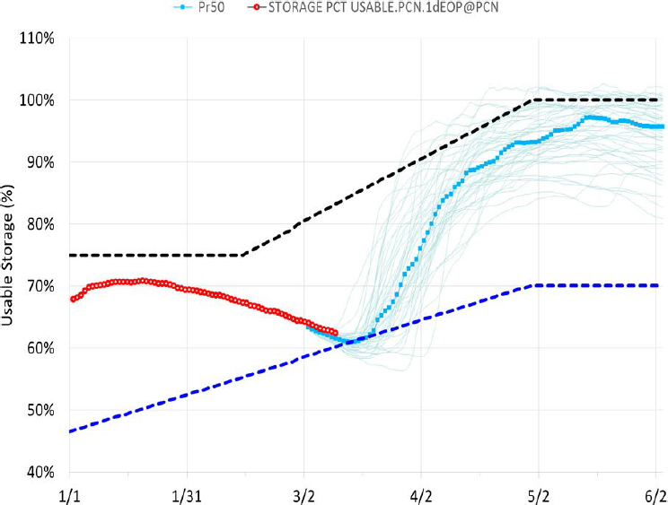
voirs (Pepacton, Cannonsville, and Neversink or “PCN”) during winter and spring 2015. Defined by PCN combined storage relative to a seasonally varying rule curve, the thresholds for drought watch are based on historical data and hardcoded in OST (Porter et al., 2015). Projected PCN storage relative to the upper storage zone (black line) and the drought watch rule curve (blue line) is shown in Figure 2-6, in which the x-axis represents time (month/day) in 2015. The complete ensemble (with all traces) is shown, with the ensemble median in red. Each trace provides a time series of simulated reservoir storage level for 365 days (if that duration is selected) from the present day. This figure was generated by an OST model run on January 2, 2015, and all of the projections indicated that PCN storage would
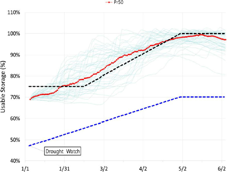
increase into the upper storage zone, refilling PCN by mid-May. Notably, none of the ensemble members approached the drought watch threshold.
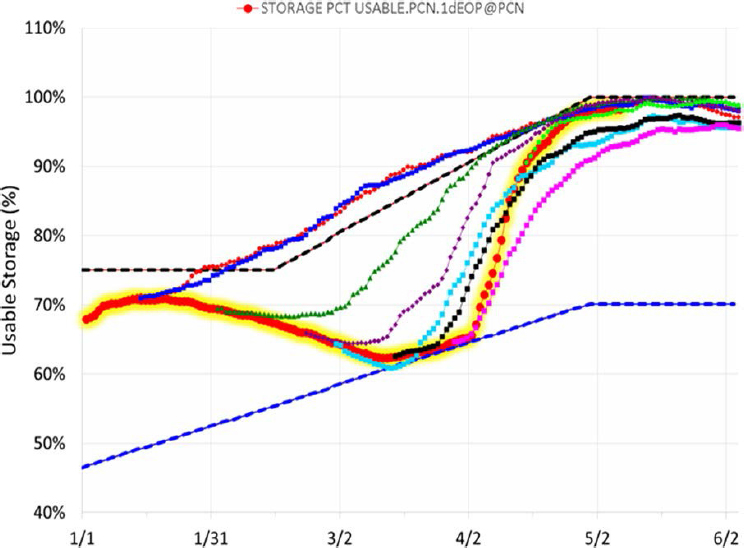
Subsequent cold temperatures and the lack of snowmelt and/or rain events led to declining streamflow and reservoir storage volume. Selected OST projections approximately two weeks apart indicated declining storage levels approaching the drought watch line for several weeks, followed by eventual melting of the snowpack and subsequent increase in storage levels (see Figure 2-7). During this time, outside concerns regarding the PCN system going into a drought watch were increasing because of the actual storage trend (red line; Figure 2-8). Notably, the medians remained above the drought watch line while the traces that dipped below it only did so for
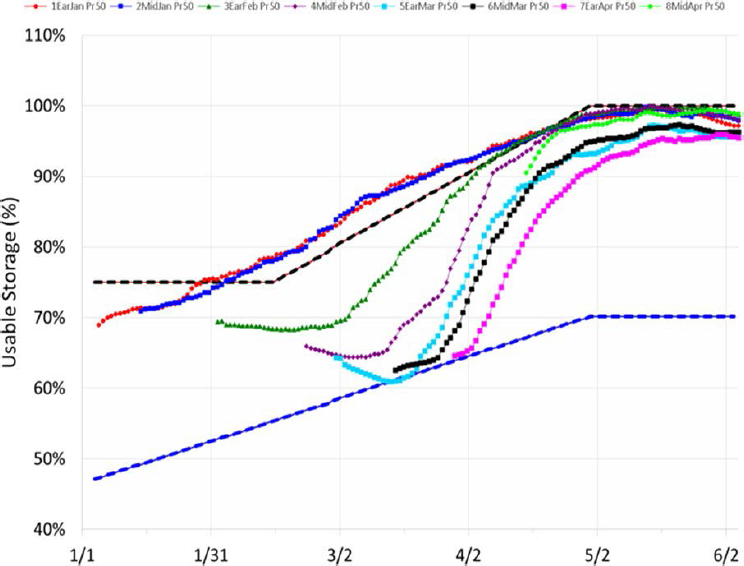
approximately one week (Figure 2-8). Figure 2-9 shows the actual storage data overlaid on the projections, indicating that the model logic in OST coupled with the ensemble inflow forecasts were able to provide operational guidance that allowed NYC DEP managers to keep PCN storage above the drought watch line. Here, having several ensemble forecasts provided more confidence in the validity of the prediction and allowed managers to implement and communicate OST-guided operational decisions with greater certainty (Porter et al., 2015).
Use of OST in Simulation Mode
OST can be utilized for longer-term planning and assessment purposes that are not focused on short-term operational decisions; NYC DEP refers to this as using OST in simulation or Sim mode. It typically involves using a single, long-term inflow trace, usually of historical hydrology or alternative hydrological time-series data, to drive the model while using a given set of operating rules.
OST can be run in Sim mode to explore the differences between such aspects as changes in the operating rules embedded in the model, physical changes to the supply system, longer-term/alternative forecasts of future climate/meteorology, or other changes. Simulations can be made with or without the W2 water quality models and with single or multiple inflow time series. For example, OST was used to simulate the impact of the Shaft
4 interconnection when that option was evaluated during the Catskill Turbidity Control Study. Simulations of Catskill Aqueduct turbidity levels and loads were used in the Catskill Turbidity Control Study to assess the impacts of various possible turbidity control measures on the estimated frequency of the need for alum addition (Weiss et al., 2013). The impact of proposed modifications to release rates can be tested using long-term OST runs looking at changes in number of drought days, effect on seasonal storage patterns in the reservoirs, and other variables of interest. Other examples may include evaluating the impacts of changing demand on the ability of the system to continue to meet demand—this includes safe yield analysis, in which different demand levels are tested to determine the point at which the system fails to meet demand. As discussed in detail in Chapter 5, climate change impacts on the water supply can be assessed by running OST in Sim mode, driven with multiple synthetic hydrology time series derived from climate change scenarios such as global climate model (GCM) downscaling, use of weather generators, and so on. Climate change mitigation strategies can be tested by running the impacted scenarios and using modified system operating rules.
OST DATA INPUT
OST is initialized with input data on a number of variables, including the current volume of storage in each of the system reservoirs, streamflows in relevant river reaches, and critical water quality conditions (such as turbidity at various points in the system). A number of near real-time internal and external data sources are used to provide some of the required input to operate OST and execute the OASIS and CE-QUAL-W2 models, especially for initial conditions for future simulations and historical data for calibration and validation of models. Indeed, one of the benefits of using OST is that it pulls in disparate data streams to enable continuous water quality and quantity management and helps to ensure that data are used, rather than remaining within bound reports.
Data acquisition and management are provided through a Water Information Systems KISTERS framework, which is a tool for time-series data management, acquisition, and visualization that interfaces with diverse data sources. This includes all OST data sources such as National Weather Service (NWS) and U.S. Geological Survey (USGS) time-series data, real-time and near-real-time sensors, laboratory information management system data, manual field entry from field personnel, and New York City’s Supervisory Control and Data Acquisition (SCADA) systems (NYC DEP, 2010).
It is not the Committee’s intent to exhaustively describe the various types and sources of data used as input to OST, but rather to focus on the most important and uncertain inputs, which are the ensemble streamflow
forecasts from the NWS and the relationship between turbidity and streamflow. Other data inputs that are standard and unremarkable are mentioned only briefly.
Streamflow Input
OST automatically acquires current discharge information derived from a network of continuously monitored USGS stream gaging stations within and downstream of the New York City watersheds. Current discharge data are used to establish initial conditions for the models while historical discharge data are valuable for calibration and validation of model performance. The data at USGS streamgages are recorded at 15-minute intervals, stored onsite, and then transmitted to USGS offices every hour through the Geostationary Operational Environmental Satellite (GOES) operated by the National Oceanic and Atmospheric Administration (NOAA). From there the data are available through web browsers and via USGS National Water Information System web services.2
Time series of future streamflows are a major input into OST. As previously noted, a single time series of streamflow is a trace, while a group of multiple time series starting at the same time is an ensemble. NYC DEP utilizes OST to consider the impact of a range of possible future inflow scenarios on water system operations. The methods for developing the streamflow forecast ensemble have evolved over time; they are presented here in order of increasing complexity. Although OST can utilize ensembles from each of the approaches considered here, the primary approach used in OST is HEFS.
As shown in Figure 2-3, the ensemble streamflow forecasts go through a forecast processor that is comprised of several modules. One of those modules is the Ensemble Post-Processor version 2, which adjusts the forecasts to (1) account for the fact that NWS forecast points are not co-located with OST nodes, (2) address systematic bias, and (3) integrate current (last 30 days) snow data into the forecast predictions. Six additional modules within the forecast processor address demand, forecast aggregation, turbidity, and other hydrologic forecasts, and then the processed information is passed to the OASIS model. The forecast processor is not the subject of the following section, but rather the streamflow ensembles received from the NWS.
Historical Records Approach
In the historical records approach, all years in the historical record are considered to be equally likely inputs going forward. One advantage of
___________________
this approach is that it preserves the intersite spatial correlation structure of the streamflow records at all of the sites, a very important feature of the data. The importance of spatial correlations is illustrated by the variability in drought severity of different watersheds within the entire NYC water supply system. Managers can draw supplies heavily from some basins where the drought may be less severe and less so from those parts where it is more severe. Taking advantage of the spatial variability of drought conditions is like portfolio diversification. Given the importance of this spatial variability, getting an accurate representation of the cross-correlated structure of the hydrologic variables is crucial to having a meaningful ensemble forecast set.
The historical records approach also captures the serial correlation3 of the streamflow (at all timescales from daily to seasonally). This serial correlation structure is a critical ingredient to estimating the risk of shortage. It describes the propensity of drought conditions or wet conditions to persist. Drought management strategies depend on having a good characterization of serial correlation. There is a vast literature on how to characterize this dependence structure at short timescales as well as the long-term persistence of streamflow data (for discussions of these issues, see Hurst, 1951; Mandelbrot and Wallis, 1968; Klems, 1974; Koutsoyiannis, 2002; Cohn and Lins, 2005). The historical records approach avoids the controversial question of what is the proper way to build a statistical model of this serial dependence and simply uses the empirical records to represent it. It avoids model error but it confines the forecasts of future conditions to be based only on the particular sequence of events that have happened in the past, rather than generating a wide range of possible outcomes using Monte Carlo simulation approaches. The serial correlation structure and spatial correlation structure are critical ingredients for estimating the risk of shortage. It is a great advantage of the historical records approach that it does not require a set of simplifying assumptions about either the spatial or serial correlation structures. Any statistical model used for ensemble forecasting will never fully capture these patterns.
What the historical records approach fails to capture is, first, the current state of the watershed’s hydrology. In particular, if conditions are wet due to a prolonged period of high precipitation, this has a large influence on the probability distribution of flows going forward. When conditions have been wet, there is essentially no chance of extreme low flows in the days or weeks going forward. The historical records approach only provides the marginal probability distribution. What is needed for risk estimation
___________________
3 Serial correlation is a statistical measure of how much the streamflow on any given day depends on the streamflow on some previous day. A good forecast must properly represent this aspect of the behavior of daily streamflow.
purposes is a conditional probability distribution of streamflows, based on the recent flow history. The historical records approach fails to capture the conditional distribution information.
The historical records approach also does not capture any information about snow and ice conditions in the watershed. Clearly, in a year when snowpack is large, the conditional distribution of streamflow in the coming months will tend to be above normal. Ice conditions (e.g., frozen soil) can also be of great importance in terms of how the watershed may respond to precipitation events in the next few days (a larger than normal fraction of the precipitation may run off if the ground is frozen). None of this information is available in the historical records.
The historical records approach also does not capture the information in weather forecasts. At timescales where there is substantial forecast skill (up to 7 days), the conditional distribution of precipitation is likely to depart substantially from the marginal distribution. For example, there may be a drought, but the weather forecast indicates that substantial precipitation is likely in the next few days. A model that uses the forecast will result in estimated reservoir storage conditions that may be fairly high seven days hence, whereas a model that does not use the forecast will produce a very broad range of storage conditions. Assuming that the model produces an accurate representation of the conditional distribution of precipitation over the coming days and weeks, it will help the outputs become more realistic and lead to better management decisions.
At this time, there does not appear to be interest (within NYC DEP) in using the historical records approach to generating ensemble forecasts. That is a reasonable decision in light of the fact that other tools are now available that make use of weather forecast information and also snow condition information. However, there remains some value to having the capability to use a historical records approach given its simplicity (e.g., there may be reasons why some of the modeling tools might be temporarily unavailable) and as a general approach for checking the results of much more sophisticated methods. One may want to explore how the system would respond to a “replay” of some extreme conditions from the past (for example, 2011, which includes Hurricane Irene, or the multiyear drought of the late 1960s). The historical records approach makes that possible. The historical records approach provides a kind of baseline approach to forecasting that can be used to help benchmark the more sophisticated approaches. The OST software does make it possible to use the historical records approach.
Conditional Forecast Approaches
The conditional forecast approach also uses the historical records of inflows, but it uses them to build a stochastic model that attempts to cap-
ture the spatial and temporal correlation structure of the observed data. By doing this it overcomes the first drawback of the historical records approach previously mentioned (capturing information about the current hydrologic state of the watershed). It takes advantage of information about the current state of the watershed by using the streamflow record as a surrogate for more meaningful (but more difficult to collect and summarize) state variables such as soil moisture and groundwater levels.
There are two conditional forecast methods that are available for use in OST, known as the Hirsch method and the eHirsch method. The first of these is taken directly from a method described by Hirsch (1981). It is a stochastic model of streamflow at a monthly time step. It operates by initializing the model using flow data for the most recent months and then generating multiple realizations that preserve the observed month-to-month correlation structure and overall properties of the probability distribution for future months based on the historical records. The eHirsch method is simply an extension of the Hirsch method, defined for a shorter time step.
The strength of this approach is that it preserves the annual cycle of the central tendency, variability, and distributional form that is observed in the historical data, as well as the serial correlation structure. The weaknesses are that it does not consider meteorological forecasts (at any timescale) and does not consider the watershed snowpack storage conditions. Adding snowpack information could be considered but it would require adding a good deal of complexity to what is otherwise a rather simple model. It would begin to move it more in the direction of a physically based forecasting model, rather than one that is entirely statistical.
An advantage of this type of stochastic model is that it will prevent simulations that include an overly rapid shift from high streamflow to very low streamflow but will allow low streamflow to shift rapidly to high streamflow. This characteristic is crucial to creating a realistic ensemble streamflow forecast. The current month’s flow determines a “floor” for the future month’s flow based on how the soil and groundwater system will deliver water to the stream when precipitation is minimal. The stochastic model, including the distribution of the random component of the model, ensures that this base-flow recession behavior is approximately preserved. The model behavior is not symmetrical, which is how it should be. The occurrence of high precipitation in a future month can restore streamflow from low values to very high ones. The distribution of the random inputs, derived from the historical data, ensures this. There are complexities involved in preserving the serial correlations and spatial correlations in this type of multinode model. Generally the distributions can be approximated well by using appropriate transformations of the time series at each node in the system. Such a model could be extended to include the modeling of particulate matter (turbidity) in those sub-watersheds where it is important.
The relationship of turbidity to streamflow is strong, but there remains a large amount of unexplained variation in turbidity for any given streamflow that would best be handled through a multivariate stochastic model such as would be used in this situation.
The conditional forecast approach does not take advantage of weather forecast information. Again, this information can be very significant in terms of outcomes at time horizons of a few days to a few weeks, but is of relatively little consequence at time horizons on the order of months. OST uses this type of approach only as backup if the other approaches are not available.
Weather Model-Driven Forecast Approach
The third approach is driven by weather-model outputs used in conjunction with a model of watershed hydrology. This approach overcomes both of the drawbacks mentioned for the historical records approach. It incorporates the memory of the initial conditions of watershed hydrology, and it takes advantage of the meteorological forecast skill that can be very substantial at short lead times. The issue with this approach is the very large number of assumptions involved in modeling the system. Here, one must start with precipitation and temperature ensemble forecasts distributed across the landscape. Producing these requires a wide range of assumptions about spatial structure and temporal structure of these processes and potential biases of the models that produce the temperature and precipitation time series. Then, there are the many parameters and assumptions involved in a distributed watershed model. Validation of this entire modeling system is a very challenging job, which includes examining biases and distributional forms and obtaining the right representation of uncertainty in model outputs for those variables that are a few days forward in time as well as those with lead times of many months. This is a very complex task, but it must be dealt with if the results are to be used in a way that captures the true uncertainty. This is the approach recently integrated into OST.
Hydrologic Ensemble Forecast Service. The primary forecast tool now used in OST is HEFS. The meteorological inputs to HEFS use a combination of three different systems (each for a different forecast lead time), which are then blended together to form a single forecasting method. The forecasting system is designed to create a set of ensemble forecasts of temperature and precipitation. At lead times of 1 to 16 days, these are generated by the Global Ensemble Forecast System (GEFS), which is a numerical weather forecast model. At lead times of 17 to 270 days, it uses another numerical weather forecast model, the Climate Forecast System version 2 (CFSv2). For days 271 to 365, it does not use a numerical weather forecast
model; instead it uses historical climatology. Evaluating these three approaches and evaluating the way that they are blended to produce a unified forecast product for the many spatial points and for days 1 to 365 is well beyond the scope of this review.
A crucial component of the HEFS system is the Meteorological Ensemble Forecast Processor (MEFP) (Demargne et al., 2014; NWS, 2016). MEFP merges these different types of forecasts in time, producing realistic forecast traces that are unbiased and have the right degree of uncertainty. The method for doing this merging is called the “Schaake shuffle” (named for J. Schaake, former director of the NWS Hydrologic Laboratory, who was an early innovator in the field of ensemble hydrologic forecasting). A detailed discussion of how the Schaake shuffle operates is found in Clark et al. (2004) and Schaake et al. (2007).
The concept used in MEFP is to take a point forecast (a single-value forecast of temperature or precipitation as opposed to an ensemble forecast) and then add an appropriate amount of uncertainty to it based on a comparison to past forecast errors and to correct for systematic biases, also based on past forecast errors. MEFP then downscales these forecasts to the individual hydrologic basins to be simulated. For example, if the point forecast of precipitation for some 6-hour period that lies a few days in the future indicates a relatively large amount of precipitation (for that location and that time of year), the MEFP uses a statistical representation of the correspondence of past forecasts (for the appropriate season, forecast location, and forecast lead time) and actual outcomes from those forecasts to describe a conditional probability distribution (which is called the conditional probability forecast) of precipitation for that six-hour period. That conditional distribution captures what is known about the natural variability of precipitation and the skill of the forecast. However, hydrologic models require an actual time series of precipitation and temperature for each modeled basin. They can not be run directly from a conditional probability forecast. MEFP uses the actual history of precipitation and temperature conditions for that basin and time of year, and randomly samples from the distribution of those records in a way that captures the mean and variance of the conditional probability forecast for each time step going forward from the time the forecast is being made. The method is an innovative blend of modern weather forecasting technology with a highly data-driven approach that preserves spatial and temporal correlation in the variables.
The hydrologic simulation component of the HEFS system uses two different watershed models to cover the NYC watershed. For the portions of the system that drain to the Hudson River, the hydrologic model is the Sacramento Soil Moisture Accounting Model (SAC-SMA) (Burnash et al., 1973), which is run by the New England River Forecast Center. This hydrologic model is used by 12 of the 13 River Forecast Centers across the
United States. For the portions of the system that drain to the Delaware River, the hydrologic model is the Continuous Antecedent Precipitation Index (API) model (Sittner et al., 1969), which is run by the Mid-Atlantic River Forecast Center, the only river forecast center to use this model (see Restrepo, 2017). The Continuous API model is commonly viewed in the hydrologic modeling community as best suited to the simulation of flood events, but not well suited to simulation of low-flow or drought conditions because of how the model was calibrated. When asked why the two different model systems were used in the two different parts of the overall New York City watershed, the NWS representatives answered that these were the models that each of the two river forecast centers was most familiar with. There was no indication that any testing had occurred to determine if the use of these two different models results in any type of differential bias between the two parts of the watershed. The Committee is concerned that the use of two different model types may result in a geographic bias in the results, and that accurate simulation using the Continuous API model during prolonged droughts might be an issue. Given that the use of HEFS overall must focus both on risks associated with high streamflow as well as with prolonged low streamflow, the use of API seems to be a potentially serious weakness in the current modeling approach, unless the model can be shown to properly handle estimation of low-flow conditions and does not diverge from the results derived from the Sacramento model.
Another concern with the HEFS approach undertaken here is the fact that the historic precipitation and temperature records used by MEFP to create the ensemble of inflow traces fails to consider any hydrologic conditions during the past 20 years. The period of record used in creating the ensemble traces covers the period 1950 to 1997. Even if climate change were not a topic of concern, it is problematic to not use an additional 20 years of historical experience (see Box 2-2 for a comprehensive explanation of this concern). But considering concerns over climate change and the fact that there is already evidence of changes in precipitation intensities, temperatures, and (as a consequence) streamflow, this omission is particularly troublesome. The Committee’s analysis, discussed in Box 2-2 and shown in Appendix A, is that the HEFS (and hence OST, which depends on it) will simulate low-flow conditions that are about half the discharge values that would be simulated using the more recent record. Precipitation patterns have changed in this region in recent years, and the HEFS simulations must be biased low because they are based on an earlier and dryer period of record. Adding the more recent data is vital to keeping the simulations aligned with current climate and hydrology conditions that may be a better indicator of future conditions.
A further concern with the HEFS approach is that the CFSv2 forecasts are used even though they could not be shown to provide any more forecast
skill that what would come from using the historical climate data. This was demonstrated in several of the graphics presented to the Committee that showed precipitation forecast skill falling to zero in six to ten days (Brown, 2017). That being the case, it would seem that the much simpler approach of using historical climate data would be preferable. The forecasts would still benefit from the hydrologic model forecast skill, but the precipitation forecasts add nothing beyond about the first ten days. As part of the North American Multi-Model Ensemble (NMME) system (see Kirtman, 2014), CFSv2 is available at a 1-degree resolution along with other models. That is, NMME offers a suite of other models that can provide a multimodel system. Whether these together, as a super-ensemble, offer skill for the NYC DEP is unknown, but should be explored by the agency.
A new tool for ensemble streamflow forecasts that has come into existence since OST was developed is the National Water Model.4 The National Water Model, which is evolving rapidly, simulates weather at local scales throughout the United States and currently operates four different versions that vary in forecast range and the frequency of updates. Should NYC DEP decide to consider alternative ensemble forecasts that offer more state-of-the-art models than those provided by the River Forecast Centers, it should only do so after validation efforts have been undertaken for National Water Model outputs for the New York City watershed region.
Finally, there is one additional concern about the HEFS approach: the weather forecast product that is the first step in this process is a single-value forecast. That is, it gives a best estimate (which may be a mean or a median forecast) and then uses a model of the uncertainty about that point forecast to generate a conditional distribution at every time step for every variable. There are other forecast models that generate ensembles of precipitation and temperature rather than having to go through this additional step of estimating the conditional distributions and then “stitching” them together using the MEFP (as described in Box 2-2). The Committee is concerned about the complexity and uncertainty that arise from starting with a point forecast (such as an ensemble mean from GEFS) and “creating” a set of consistent ensembles, rather than going directly to an ensemble approach. The current approach requires building a statistical model of the relationship between the point estimate and the distribution, whereas direct use of the ensemble uses the data themselves rather than depending on a model of the relationship.
For example, NYC DEP could use the ensemble set already provided as part of the output from the GEFS run from NOAA’s Earth System Research Laboratory in Boulder, Colorado. However, the resolution is coarser than the National Centers for Environmental Prediction’s (NCEP’s) operational,
___________________
deterministic global weather forecast model Global Forecast System, which has a horizontal resolution of 28 km for week one and 70 km for forecasts between one week and two weeks. Alternative single-forecast models also include the North American Mesoscale Forecast System, which is one of the major weather models run by NCEP for producing weather forecasts over the North American domain. Its horizontal resolution is 4 km with forecasts every 3 hours going out to 84 hours. A careful analysis would be required before shifting from using a “constructed” set of ensembles around a point forecast, generated based on the statistical uncertainty of the forecast relative to observations, to using the ensembles produced from other sources.
Water Quality Input Data
Water quality information used in OST is collected in real time, in near real time, and through grab samples analyzed in a laboratory. Real-time data are collected at critical locations within the watershed through the New York City Keypoint Monitoring Program (NYC DEP, 2010). Currently, real-time data are collected and managed separately for West of Hudson (WOH) and East of Hudson (EOH) operations. Real-time data for both WOH and EOH operations are transmitted via telemetry. The WOH data are available in real time to supply operators in the New York City Water Supply Control Center. In contrast, only the New Croton Reservoir of the EOH data system is currently viewed and archived through a SCADA system, but plans are in place to include all EOH reservoirs within the SCADA system in the near future (NYC DEP, 2010).
Near-real-time data of turbidity, temperature, conductivity, and dissolved oxygen are collected at in-reservoir sampling buoys at select reservoirs. This information is transmitted telemetrically and distributed via file transfer protocol for subsequent viewing and archiving. Laboratory samples through both the Keypoint sampling and reservoir grab sampling are processed, analyzed, and managed by the New York City LIMS (NYC DEP, 2010), and are accessed automatically by OST through the LIMS Web interface for model initialization (NYC DEP, 2010).
Turbidity of Future Streamflows
It is a common practice in water quality studies to build regression models of water quality variables (such as turbidity or TSS) to streamflow along with additional explanatory variables related to time of year and long-term trend. These models are discussed extensively in the literature, for example, by Cohn et al. (1992) and Cohn (1995). The relationship between turbidity and streamflow has been studied by Mather and Johnson (2014)
in general and by Mukundan et al. (2013), Ahn et al. (2017), and Ahn and Steinschneider (2018) in the NYC DEP watershed.
The regression models developed by NYC DEP for predicting the turbidity of reservoir inflows are particularly important in the Catskill system, where the watersheds are susceptible to mobilization of turbidity as streamflow increases. Season of year and antecedent conditions also affect inflow turbidities. NYC DEP has developed regression models for turbidity as a function of tributary flow for Schoharie Creek as well as for two locations on the Upper Esopus Creek, one just upstream of the Shandakan Tunnel inflow (Allaben) and one just upstream of Ashokan Reservoir (Coldbrook). Approaches to date for regression development have included simple empirical regressions of log (turbidity) versus log (flow), more complex best-fit deterministic (BFD) regressions, and multiple event-specific regressions. For use of OST in PA mode with W2 turned on, the simple empirical regressions are used because the BFD regressions require information not readily available for future forecasts, such as event-specific peak flow, antecedent dry period, and date of peak flow. NYC DEP is exploring use of time-varying regressions to capture the inherent variability in sediment susceptibility to erosion for a given flow condition. Results for dynamic linear regression modeling of suspended sediment versus flow have recently been reported for the Catskill watershed (Ahn et al., 2017; Ahn and Steinschneider, 2018). NYC DEP has indicated that it is first exploring use of such an approach outside of OST prior to possible use within OST. The applicability is for shorter-term (one-day to one-week) forecasts, not long-term forecasts. Some of the coefficients in the dynamic linear regressions can be interpreted as reflecting the changing likelihood of sediments being eroded and transported (Asselman, 2000).
Figure 2-10 shows the simple regression relationship between Schoharie Creek turbidity and streamflow with no other parameters considered. This relationship was developed during the Catskill Turbidity Control Study. Figure 2-11 shows the turbidity-flow relationship for the Upper Esopus Creek at Coldbrook as used within OST in PA mode, also developed as part of the Catskill Turbidity Control Study. The data in both figures show about an order of magnitude variability in turbidity for a given streamflow. As previously noted, this is a result of the impacts of time of year (e.g., winter versus summer), antecedent conditions (e.g., especially dry or wet recently), and rate of change of discharge (hysteresis) on sediment erosion that are not captured by the magnitude of flow alone.
To better understand the overall role of uncertainty in the entire OST process, it seems appropriate for the model formulations used for simulating turbidity loads to the reservoirs to include some component that represents the uncertainty of estimates of turbidity that are produced from the discharge-based regression models. This should include questions about
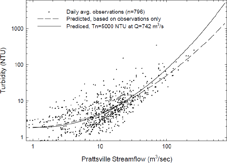
whether the error variance is constant over time, over the range of discharge, or across seasons. Methods suitable for conducting such analyses exist currently (e.g., Hirsch et al., 2010; Hirsch and DeCicco, 2015). During the Catskill Turbidity Control Study, the NYC DEP conducted some analyses of the uncertainty in the flow-turbidity relationships (such as Monte Carlo analysis using multiple event-based regressions). The Committee encourages NYC DEP to evaluate if the discharge-turbidity relationships have changed over time, and if there is any seasonality to these relationships. The Committee encourages use of regressions based on inclusion of the most recent data, especially data for more recent high-flow events, and further evaluation of the potential impact of high tributary inflow turbidity on Kensico diversion turbidity.
Meteorological Information
Meteorological data (precipitation, air and dew point temperatures, wind speed and direction, cloud cover) are collected through NWS surface weather forecasts and are utilized in the CE-QUAL-W2 water quality
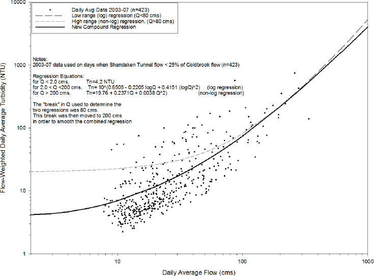
models. Additional meteorological and snow depth data are collected from New York City’s own network of meteorological stations and transmitted telemetrically.
VALIDATION OF OST
Validating an end-to-end system such as OST is no simple matter, and it is not clear that the statistical literature has a lot of advice to give about this process. Moving away from single-value forecasts and rigid use of rule curves is clearly the right thing to do for informing water management and operations. Nevertheless, validation5 remains a challenge for this system.
___________________
5 The terms “validation” and “verification” are often used interchangeably in the hydrologic modeling arena, and the Committee considers them synonymous in the context of this report (see Appendix C). The Committee uses the term “validation” throughout for consistency, although citations and other users, such as the NWS, may embrace the other term.
Ensemble Streamflow Forecasts
Validation of the ensemble streamflow forecasts includes examination of biases, distributional forms, and obtaining the right representation of uncertainty in model outputs for those variables that are a few days forward in time as well as those with lead times of many months. This is a very complex task, but it must be dealt with if the results are to be used in a way that captures the true uncertainty.
The question is, how does one judge the quality of models designed to estimate conditional probability distributions? Most atmospheric and hydrologic forecast modeling has been focused on the question of the accuracy of a point estimate. For example, how well does the model predict the instantaneous maximum discharge value of a flood hydrograph that results from a given storm? Or, what is the expected value of streamflow volume entering a reservoir over the upcoming month? One can use metrics such as root mean squared error or Nash-Sutcliff efficiency or some other loss function to evaluate alternative strategies for making these forecasts. The problem confronted here is quite different from those. Rather than being interested in questions such as how much difference is there between the forecasted value (perhaps a mean, or median, or most likely value of some random variable) and the true outcome, what the NYC DEP should be interested in is the accuracy of the conditional probability distributions that are generated by OST. How well do they represent the true distribution of outcomes? Understanding the accuracy of the range of outcomes is critical to being able to provide accurate assessments of the probabilities of certain types of bad outcomes discussed earlier in the chapter. This question is complicated by the fact that this conditional distribution is different each time the ensemble forecast is made.
Consider two hypothetical situations in which the forecasting method might be considered to work poorly. Assume here that the random variable of interest is streamflow volume entering a reservoir over the next 30 days. What if the outcomes are frequently (for example, 60 percent of the trials) found to be below the 10th percentile or above the 90th percentile of the forecasted conditional distribution stated at the start of that 30-day period? Then one can conclude that the conditional distributions were too narrow. In other words, managers are given a false sense of certainty about the next 30 days. A consequence of this is that actions designed to avoid bad outcomes in either direction (too wet or too dry) are not given an appropriate degree of consideration in operational decisions. Conversely, what if outcomes are frequently (for example, 80 percent of the trials) between the 40th and 60th percentiles of the conditional distribution estimates? In this case the model is seriously overstating uncertainty and actions taken to avoid upside or downside risks are overemphasized. Conducting ex-
periments using the forecasting method and the data on actual outcomes provides valuable information to the user and the modeler as to how well the forecasting system is working. It should also be able to provide insights on how the forecasting system should be modified and then used again to verify that the modifications are moving performance in the right direction.
Fortunately, there is some literature that considers this type of validation problem and lays out appropriate strategies and metrics. The methods described by Bradley et al. (2004) are known as distributions-oriented verification of ensemble streamflow prediction. Some of the metrics described by Bradley et al. (2004) include the Brier score (Brier, 1950), relative resolution, relative reliability, and relative sharpness (see also Krzysztofowicz and Herr, 2001; Wilks, 2011). The methods exist for doing these types of validation of ensemble forecast products. NYC DEP and other interested parties need to be mindful that assessment of the accuracy of point forecasts (e.g., statements that the expected discharge at some node in the system seven days in the future will equal some specific value) are not appropriate for determining the quality of the forecasts that are being produced for OST. Rather, the validation approaches need to focus on the degree to which the ensemble forecasts correctly capture both the central tendency and the variability of the conditional probability distributions.
In presentations to the Committee in late 2017 there were descriptions of work in progress aimed at validation of HEFS forecasts in general (not limited to those for the New York City watersheds) and for the forecasts that are specific to OST. However, as of the end of 2017, no published results of these efforts were available to share with the Committee. Of particular importance is the need for validation to help make trade-offs between high levels of method complexity and parsimonious approaches with much more limited data requirements and more limited sets of assumptions. It is natural to favor the more complex approaches because they are able to represent a wide range of important processes and use important input variables. However, decisions on these trade-offs need to be informed by validation studies rather than by the comfort level of the practitioner. Pursuit of these types of studies is important to the quality of the OST tool going forward and important to maintaining trust in the process within NYC DEP management and in the stakeholder community.
Use of Hindcast Mode for OST Validation
Mathematical models of complex physical systems are commonly run forward in time in a forecast mode in order to gain insight into how the presently configured system will respond to projected future conditions. This is how NYC DEP uses OST when it conducts its frequent runs of OST in PA mode and in Sim mode. However, simulation models are frequently
run to simulate the past (hindcast mode), especially for the purposes of model development and validation. These events can be represented with actual observations of both model inputs and actual outcomes. The purpose of running a model such as OST in hindcast mode is to see how well the model performs, that is, whether the output of the model matches outcomes that were actually observed. Divergence between model output and historical observations is a measure of a model’s skill at capturing the behavior of the physical system with sufficient fidelity to place confidence in its results. Hindcasting provides one of the most powerful means of testing the validity of a simulation model’s mathematical structure and underlying assumptions (see, e.g., Karna and Baptista, 2016).
In the case of OST, hindcasting can refer to a variety of approaches because of the many components of OST that can be manipulated and examined. For example, one could run the model as if it were the past using observed streamflow, demand, and turbidity data as input and then compare model outputs to actual diversion, release, and turbidity observations. Other hindcasts could be conducted in which the system operations are scheduled or somewhat scheduled to be identical to what they were during the past, in order to then compare simulated turbidity outputs to actual observations of turbidity. These different approaches would invariably be testing the validity of different process representations within OST.
At its meeting in April 2017, NYC DEP staff presented multiple and early efforts for validating OST that made it clear that they were aware of the complexity of the task. As NYC DEP moves forward with these efforts, it will be important for the modelers to describe exactly which parts of OST are being tested by a given validation method. Beyond the exercises that NYC DEP has already attempted, the Committee suggests that NYC DEP stress test the performance of the system as currently configured using historical records of extreme events. One analysis could examine system performance under an extended drought scenario on the scale of or even larger than the drought experienced in the 1960s. Another could examine how OST simulation of system conditions compares to actual conditions that resulted in response to the sequential rainfall events of Hurricanes Irene (August 21–28, 2011) and Lee (September 1–5, 2011). Results could reveal both the strengths and weaknesses of OST’s representations of streamflow and turbidity under a wide range of stressful historical conditions.
CONCLUSIONS AND RECOMMENDATIONS
OST is one of the most advanced and complex support tools for water supply operations in the world. The Committee regards the NYC DEP as a leader among water resource agencies nationwide at applying these types of tools to inform system operations. The Committee strongly endorses the
use of probabilistic forecast tools to inform NYC DEP’s management decisions, allowing it to explicitly balance the risks of water shortage against the risks of having too much water (and the turbidity issues that come with high-flow events). Moving forward, OST offers a dynamic water routing platform that is both adaptable and capable of continuous improvement if properly resourced with data, validation, and most importantly, continued maintenance and growth of institutional expertise. The following conclusions and recommendations are intended to bring about improvement in the ability of NYC DEP to make better use of OST now and in the future.
The historical data used in HEFS to create the ensemble streamflow forecasts need to be updated now to include the most recent 20 years, and this updating needs to occur on a regular schedule into the future. There are important trends from the last 20 years that are not being captured by use of data only from 1950–1997, as shown in detail in Appendix A. In light of the changes in climate and resulting hydrology in the region that are already underway, it is crucial that the climate data that drive the ensemble forecasts be kept up to date. The HEFS system must adapt to a changing climate, and that is not possible if the data used are 20 years out of date. Updating these data to near present is imperative now, and a plan for a regular cycle of updates should be a part of the HEFS system inputs to OST.
NYC DEP and the NWS, which operates the weather and hydrologic forecasting model components of the system, need to critically evaluate the appropriateness of each of the key components of the ensemble streamflow forecasts. The hydrologic model used by the Middle Atlantic River Forecast Center, Continuous API, is not state of the art, and serious consideration should be given to replacing it with the Sacramento Soil Moisture Accounting Model (SAC-SMA) that is used by all other River Forecast Centers. CFSv2 appears to provide no precipitation forecast skill (beyond about ten days), such that the Committee questions its use in OST. An approach driven by historical climatology would entail far fewer assumptions and much more straightforward processing. When longer-term weather forecast models can be shown to provide significant skill, with respect to precipitation, then it would be justified to include such models in the system.
Probabilistic validation results for the ensemble streamflow forecasts need to be published for the New York City watershed region. The Committee does not recommend traditional validation on point estimates, but rather on the conditional distribution of the ensemble. The Committee understands that the NWS has a set of appropriate, ensemble validation exercises underway at present. The Committee urges NYC DEP and the
NWS to publish these results and provide for a continuing set of validation products.
The NYC DEP should continue in its efforts to update the streamflow-turbidity relationships and include their uncertainty. The Committee recognizes that including additional ensembles of turbidity inputs, representing the uncertainty of turbidity level traces for any given streamflow trace, would add a great deal of computational time and complexity to the OST model. However, updating the streamflow-turbidity relationships to be based on the most recent data, to reflect recent trends, and to determine if there is any seasonality in these relationships would be valuable and could result in some improvements to the OST approach.
The Committee encourages the NYC DEP to examine the sensitivity of OST simulations to the values of the weights and penalties assigned within the OASIS model. The capability of OASIS to simulate the decisions that would be made by expert system operators is likely to depend on the values of the weights assigned to different flows and reservoir volumes, which reflect relative priorities of system performance (e.g., water storage volume, water quality, and water releases). Understanding and communicating the sensitivity of model outputs to decision variable weights should improve model performance and the confidence of stakeholders in the model simulations.
The Committee encourages the NYC DEP to continuously improve OST so that it remains operationally relevant, particularly in the face of growing environmental pressures such as climate change and more stringent regulations. Since its inception, the institutional memory and expertise of NYC DEP staff have been critical to refining the numerous data inputs, representing the operational complexities of the water supply, and weighting the various model components within the OST framework. The biggest risk to OST failing to fulfill its role as a water management decision support tool is a lack of continuous improvement, knowledge transfer, and knowledge mobilization through succession planning to ensure that the best and most appropriate data and operational insights are used to inform the inputs, the models, and the other relationships that OST relies upon.
REFERENCES
Ahn, K.-H., and S. Steinschneider. 2018. Time-varying suspended sediment-discharge rating curves to estimate climate impacts on fluvial sediment transport. Hydrological Processes 32:102–117.
Ahn, K.-H., B. Yellen, and S. Steinschneider. 2017. Dynamic linear models to explore time-varying suspended sediment-discharge rating curves. Water Resources Research 53:4802–4820.
Asselman, N. 2000. Fitting and interpretation of sediment rating curves. Journal of Hydrology 234(3):228–248.
Bradley, A. A., S. S. Schwartz, and T. Hashino. 2004. Distributions-oriented verification of ensemble streamflow predictions. Journal of Hydrometeorology 5(3):532–545.
Brier, G. W. 1950. Verification of forecasts expressed in terms of probability. Monthly Weather Review 78(1):1–3.
Brown, J. 2017. The Hydrologic Ensemble Forecast Service (HEFS): A new era of water forecasting at the National Weather Service. Presentation to the NASEM Committee to Review the New York City Department of Environmental Protection Operations Support Tool for Water Supply. September 25, 2017, Kingston, NY.
Burnash, R. J. C., R. L. Ferral, and R. A. McGuire. 1973. A Generalized Streamflow Simulation System—Conceptual Modeling for Digital Computers. Sacramento, CA: U.S. Department of Commerce, National Weather Service and the California State Department of Water Resources.
Clark, M., S. Gangopadhyay, L. Hay, B. Rajagopalan, and R. Wilby. 2004. The Schaake shuffle: A method for reconstructing space–time variability in forecasted precipitation and temperature fields. Journal of Hydrometeorology 5(1):243–262.
Cohn, T. A. 1995. Recent advances in statistical methods for the estimation of sediment and nutrient transport in rivers. Reviews of Geophysics 33(S2):1117–1123.
Cohn, T. A., and H. F. Lins, 2005. Nature’s style: Naturally trendy. Geophysical Research Letters 32(23):1–5.
Cohn, T. A., D. L. Caulder, E. J. Gilroy, L. D. Zynjuk, and R. M. Summers. 1992. The validity of a simple statistical model for estimating fluvial constituent loads: An empirical study involving nutrient loads entering Chesapeake Bay. Water Resources Research 28(9):2353–2363.
Cole, T. M., and S. A. Wells. 2002. CE-QUAL-W2: A Two-Dimensional, Laterally Averaged Hydrodynamic and Water Quality Model, Version 3.1. User manual. U.S. Army Corps of Engineers, Instruction Report EL-02.
Cole, T., and S. A. Wells. 2015. CE-QUAL-W2: A Two-Dimensional, Laterally Averaged, Hydro-Dynamic and Water Quality Model, Version 4.0. User Manual. Portland, OR: Department of Civil and Environmental Engineering, Portland State University.
Delaware River Basin Commission. 2018. Dates of DRBC-Declared Drought. http://www.state.nj.us/drbc/hydrological/drought/drbc-drought.html#1.
Demargne, J., L. Wu, S. K. Regonda, J. D. Brown, H. Lee, M. He, D.-J. Seo, R. Hartman, H. D. Herr, M. Fresch, J. Schaake, and Y. Zhu. 2014. The Science of NOAA’s Operational Hydrologic Ensemble Forecast Service. Bulletin of the American Meteorological Society (Jan.):79–98.
Gelda, R. 2017. Water Quality Rules in OST. Presentation to the NASEM Committee to Review the NYC DEP Operations Support Tool. September 25.
Gelda, R. K. and S. W. Effler. 2007. Modeling turbidity in a water supply reservoir: Advancements and issues. Journal of Environmental Engineering 133(2):139–148.
Gelda, R. K., S. W. Effler and F. Peng. 2012. Modeling turbidity and the effects of alum application for a water supply reservoir. Journal of Environmental Engineering 138(1):38–47.
Gelda, R. K., S. W. Effler, F. Peng, E. M. Owens, and D. C. Pierson. 2009. Turbidity model for Ashokan Reservoir, New York: Case study. Journal of Environmental Engineering 135(9):885–895.
Gelda, R. K., S. W. Effler, A. R. Prestigiacomo, F. Peng, A. J. P. Effler, B. A. Wagner, M. G. Perkins, D. M. O’Donnell, S. M. O’Donnell, and D. C. Pierson. 2013. Characterizations and modeling of turbidity in a water supply reservoir following an extreme runoff event. Inland Waters 3:377–390.
Hirsch, R. M. 1981. Stochastic hydrologic model for drought management. Journal of the Water Resources Planning and Management Division 107(2):303–313.
Hirsch, R. M., and L. A. De Cicco. 2015. User guide to Exploration and Graphics for RivEr Trends (EGRET) and dataRetrieval: R packages for Hydrologic Data (No. 4-A10). Reston, VA: U.S. Geological Survey.
Hirsch, R. M., D. L. Moyer, and S. A. Archfield. 2010. Weighted regressions on time, discharge, and season (WRTDS), with an application to Chesapeake Bay river inputs. Journal of the American Water Resources Association 46(5):857–880.
Hurst, H. E. 1951. Long term storage capacities of reservoirs. Transactions of the American Society of Civil Engineers 116:776–808.
HydroLogics, Inc., 2009. User Manual for OASIS WITH OCL™ Model Version 3.10.8, GUI version 4.6.16. December 1. http://ftp.hydrologics.net/documents/OASIS_Manual4-2010.pdf.
Karna, T., and A. M. Baptista. 2016. Evaluation of a long-term hindcast simulation for the Columbia River estuary. Ocean Modelling 99:1–14.
Kirtman, B. P. 2014. North American Multi-Model Ensemble (NMME) Status and Future Plans. American Geophysical Union, Fall Meeting 2014, abstract id. A34D-03.
Klemes, V. 1974. The Hurst phenomenon: A puzzle? Water Resources Research 10(4):675–688.
Koutsoyiannis, D. 2002. The Hurst phenomenon and fractional Gaussian noise made easy. Hydrological Sciences Journal 47(4):573–595.
Krzysztofowicz, R., and H. D. Herr. 2001. Hydrologic uncertainty processor for probabilistic river stage forecasting: Precipitation-dependent model. Journal of Hydrology 249(1):46–68.
Mandelbrot, B. B., and J. R. Wallis. 1968. Noah, Joseph, and operational hydrology. Water Resoures Research 4(5):909–918.
Mather, A. L., and R. L. Johnson. 2014. Quantitative characterization of stream turbidity-discharge behavior using event loop shape modeling and power law parameter decorrelation. Water Resources Research 50(10):7766–7779.
Mead, J. 2017. OST Demonstration: Setup, execution, and reporting with W2 models on. Presentation to the NASEM Committee to Review the NYC DEP Operations Support Tool. September 25.
Mukundan, R., D. C. Pierson, E. M. Schneiderman, D. M. O’Donnell, S. Pradhanang, M. S. Zion, and A. H. Matonse. 2013. Factors affecting storm event turbidity in a New York City water supply stream. Catena 107:80–88.
NWS (National Weather Service). 2016. Meteorological Ensemble Forecast Processor (MEFP) User’s Manual, Version: OHD-CORE-CHPS-4.4.a. May 16. http://www.nws.noaa.gov/oh/hrl/general/HEFS_doc/MEFP_Users_Manual.pdf
NYC DEP (New York City Department of Environmental Protection). 2006. Catskill Turbidity Control Study Phase II Final Report – Appendix B (Upstate Freshwater Institute), prepared by Gannett Fleming/Hazen and Sawyer, September 30.
NYC DEP. 2009. Catskill Turbidity Control Study Phase II Implementation Plan: Updates and Supporting Analyses – Appendix A (Upstate Freshwater Institute), prepared by Gannett Fleming/Hazen and Sawyer, July 31.
NYC DEP. 2010. New York City’s Operations Support Tool (OST) White Paper Prepared for the Delaware River Basin Supreme Court Decree Parties. October 8.
Porter, J. H., A. H. Matonse and A. Frei. 2015. The New York City Operations Support Tool (OST): Managing water for millions of people in an era of changing climate and extreme hydrological events. Journal of Extreme Events 2(2):1550008.
Restrepo, P. J. 2017. The United States National Weather Service real-time flood forecasting. Oxford Research Encyclopedia of Natural Hazard Science. DOI 10.1093/acrefore/9780199389407.013.12. http://naturalhazardscience.oxfordre.com/view/10.1093/acrefore/9780199389407.001.0001/acrefore-9780199389407-e-128.
Schaake, J., J. Demargne, R. Hartman, M. Mullusky, E. Welles, L. Wu, and D. J. Seo. 2007. Precipitation and temperature ensemble forecasts from single-value forecasts. Hydrology and Earth System Sciences Discussions 4(2):655–717.
Sittner, W., C. Schauss, and J. Monro. 1969. Continuous Synthesis with and API-Type Hydrologic Model. Water Resources Research 5(5):1007–1022.
USGS ORDM (USGS Office of the Delaware River Master). 2017. Agreement for a Flexible Flow Management Program. https://water.usgs.gov/osw/odrm/ffmp/FFMP2017.pdf.
Weiss, W. J., G. W. Pyke, W. C. Becker, D. P. Sheer, R. K. Gelda, P. V. Rush, and T. L. Johnstone. 2013. Integrated water quality-water supply modeling to support long-term planning. Journal American Water Works Association 105(4):E217-E228.
Wilks, D. S. (eds). 2011. Statistical Methods in the Atmospheric Sciences (Vol. 100). Waltham, MA: Academic Press.


