
Appendix D
Technical Appendixes to Select Chapters
APPENDIX D, 2-1
A BRIEF HISTORY OF POVERTY MEASUREMENTS IN THE UNITED STATES
The nation’s Official Poverty Measure (OPM), developed in the 1960s by Mollie Orshansky of the Social Security Administration, is based on research showing that, in the 1950s, the average family spent about one-third of its after-tax income on food (Fisher, 1992). Orshansky then multiplied the cost of the U.S. Department of Agriculture’s “basic” diet food plan by three to calculate poverty thresholds for families of different compositions and sizes (she used somewhat different methods for families of one and two people). Families with resources (regular money income as measured in a supplement to the Current Population Survey) below these amounts were considered to be poor. These thresholds have been adjusted for inflation every year using the Consumer Price Index. The official poverty rate is calculated in essentially the same way now as it was in the 1960s.
This approach to measuring poverty has numerous shortcomings: It is based on the now outdated assumption that families spend one-third of their post-tax income on food (today they spend less than one-half that amount); it fails to adjust for geographic differences in living costs; and, more importantly, it counts neither in-kind benefits nor refunded tax credits as income. Thus, the Earned Income Tax Credit (EITC), the Child Tax Credit, Supplemental Nutrition Assistance Program (SNAP) benefits, child care assistance, subsidized housing, and many other in-kind benefits are ignored in computing the poverty rate. It is also an absolute poverty
measure in that the poverty thresholds are updated for inflation but not for changes in the country’s standard of living.1
These problems with the OPM were considered serious enough to generate congressional interest in an improved measure. Funding from a provision in the Family Support Act of 1988, which mandated a National Research Council study of a national minimum benefit standard for the now defunct Aid to Families with Dependent Children (AFDC) Program, combined with funding from the Bureau of Labor Statistics and the Department of Agriculture, supported the work of an NRC panel of poverty experts. This panel produced an influential report, Measuring Poverty—A New Approach, in 1995.
Despite the attention generated by that panel’s report, the OPM remains unchanged for many reasons, two of which are of major importance. First, numerous pieces of legislation stipulate that cash grants are to be provided to states, cities, and school districts, and the allocation of those grants is often based on the area’s poverty rate. Changing the poverty measure used in allocation formulas would affect the distribution of money among states and local areas, substantially in some cases.
Relatedly, the official poverty thresholds (actually a variant of them) are used to determine eligibility of families for a number of assistance programs. Second, defining a poverty level requires making judgments. Given the financial stakes of determining who is poor and who is not, Congress would certainly be mired in a long and contentious debate if it sought to set new poverty thresholds or change other aspects of the official measure.
Nonetheless, following the 1995 report, analysts at the Census Bureau and the Bureau of Labor Statistics began the complicated work of implementing many of the report’s recommendations for improving the measurement of poverty. By 2011, after more than a decade of study, the Census Bureau released a new method of defining poverty. The title of the new measure—the “Supplemental Poverty Measure” (SPM)—made it clear that the federal government, and in particular the Census Bureau, was not proposing to replace the OPM with a new one, but rather adding a new measure that would advance research and provide additional information for policy discussions.
___________________
1 Because the inflation index used for the Official Poverty Measure (OPM) overstated price changes for a period, the official thresholds have actually been updated to some extent in real terms—that is, for changes in living standards. See Appendix D, 2-2, for a discussion of absolute versus relative poverty measures and the use of different inflation measures for adjusting thresholds.
APPENDIX D, 2-2
TYPES OF INCOME-BASED POVERTY MEASURES AND THE ADVANTAGES OF USING THE ADJUSTED SPM FOR POLICY ANALYSIS
Poverty measurement requires a set of decisions about the purpose and specifications of the measure. As background, Box D2-1 defines key terms in poverty measurement, such as threshold and resource concepts and whether the measure is intended to be absolute or relative. It also briefly defines types of poverty measures, including economic measures, such as those based on income or consumption, and other kinds of deprivation and hardship indexes.
The committee’s charge is to identify and estimate the benefits and costs of government policy and program options that can reduce child poverty and deep poverty in the United States within 10 years and to propose practical measures to do so given the available data. For this purpose, it is necessary to use an income-based economic poverty measure, which can clearly show the effects of one or another policy option on the adequacy of families’ resources. Other types of measures, such as deprivation and material hardship indexes, add to the picture of families’ living situations and well-being but present challenges to any straightforward estimation of the effects of government tax and transfer policies on them. This is also a limitation at present of consumption-based economic poverty measures—see Appendix D, 2-3.
The committee’s charge directs us to base our analyses on the income-based SPM and not on either the OPM or a consumption-based poverty measure. Unlike the Census Bureau, we use an adjusted SPM, in which we correct the underlying data for some types of income underreporting using the Urban Institute’s Transfer Income Model, Version 3 (TRIM3) microsimulation model. This appendix section describes and assesses the OPM, the SPM, and the adjusted SPM. It then discusses several contentious issues for income-based poverty measurement: relative versus absolute poverty; inflation adjustments; and the implications for income-based poverty, particularly deep poverty, of error in the underlying data source—the Current Population Survey Annual Social and Economic Supplement (CPS ASEC). See Appendix D, 2-3, for a discussion of consumption-based poverty measures, for which issues of relative versus absolute poverty, inflation adjustments, and data quality are also relevant.
Three Income-based Poverty Measures: OPM, SPM, Adjusted SPM
The OPM, the SPM, and the adjusted SPM used in this report are based on resources defined by a family’s income. A family is defined as poor if
family income is below a specific cutoff. The cutoff is chosen to indicate the income needed to attain a minimum or basic level of goods and services. This simple description masks the many specific decisions that are required to define an acceptable, feasible, and useful income-based poverty measure. Table D2-1 compares the OPM, the SPM, and the adjusted SPM on 11 dimensions: uses, measurement unit, threshold concept, threshold adjustments, threshold updating, treatment of health benefits and costs, resource measure, reference period, metric(s) estimated, data source, and data quality.
Three key differences between the OPM and the SPM merit fuller discussion: the type of measure (absolute or relative), the threshold concept, and the definition of family resources. Other important differences—in the adjustments to the thresholds for family composition and the unit of measurement—are briefly described in Table D2-1.
Type of measure. The OPM officially became an absolute measure in 1969, when proposals to update in real terms the original 1963 thresholds (based only on food needs—see next section) were turned down because policy makers were reluctant to show any increase in poverty.2 Since then, the thresholds have been updated for inflation only, using the flagship series published by the Bureau of Labor Statistics—the All Items Consumer Price Index for All Urban Consumers, known as the CPI-U. Overestimation of inflation in the CPI-U, however, resulted in real increases to the thresholds in the 1970s and early 1980s (see discussion of inflation indexes below).
The SPM, in contrast, is a quasi-relative poverty measure in which the thresholds are based on needs for a specific set of goods—but a broader set than food—and are recalculated every year as spending on those goods changes. It is similar to an absolute measure because the thresholds are
___________________
2 See https://www.census.gov/content/dam/Census/library/working-papers/1995/demo/fisher3.pdf. Between 1963 and 1969, changes in the costs of Economy Food Plan were used to update the thresholds.
TABLE D2-1 Dimensions of Three Income-Based Economic Poverty Measures: Official Poverty Measure (OPM), Supplemental Poverty Measure (SPM), Adjusted SPM
| Measure/Dimension | Official Poverty Measure | Supplemental Poverty Measure | Adjusted SPM |
|---|---|---|---|
| Kinds of Uses | Statistical (from 1967 in annual Census Bureau publications): —monitor trends over time and among population groups and geographic areas—see Ch. 2 Research: —study how child poverty affects child (e.g., health) or longer-term adult (e.g., employment) outcomes—see Ch. 3 —aggregate over families in neighborhoods (e.g., census tracts) to study effects on outcomes—see Ch. 8 Policy: —determine eligibility for government programs —simulate effects on poverty of existing and proposed programs and policies that affect cash income |
Statistical (from 2011 in annual Census Bureau publications): —monitor poverty trends over time and among groups (see Fox et al., 2015, for series back to 1967 using an anchored SPM); for geographic areas, the Fox et al. anchored SPM series is available by state, and some states and cities have developed SPM estimatesa Research: —too new to be used for long-term outcomes research Policy: —growing uses, which can include simulation of full range of government policies and programs that affect disposable income (e.g., tax credits, SNAP) |
Policy: —used in TRIM3 model to simulate effects of programs and policies with a more accurate income measure (see Resource Measure below) |
| Measure/Dimension | Official Poverty Measure | Supplemental Poverty Measure | Adjusted SPM |
|---|---|---|---|
| Comment: | OPM is used extensively because of its official status; ill-designed for monitoring differences among groups and areas and for policy analysis because it neglects importance sources of government income support and nondiscretionary costs (see Resource Measure below) | SPM could be used as extensively as OPM; well designed for policy analysis of effects of government benefits delivered in-kind and through tax credits (see Resource Measure below); would likely be improvement over OPM for outcomes research (although any reasonable way to identify low-income groups can work) | Same as SPM with advantage of providing a more accurate income measure (see Resource Measure below) |
| Measurement Unit | Family (individuals related by birth, marriage, or adoption co-resident in the same house) or unrelated individual age 15 or older living in a house | Resource unit (official family definition plus any co-resident unrelated or foster children under age 18, or unmarried partners and their relatives) or other unrelated individual age 15 or older | Same as SPM |
| Comment: | Does not define poverty for unrelated children in a house (e.g., foster children) under age 15; does not include anyone living in an institution (e.g., prison) or who is homeless. These limitations are inherent in the underlying data—see Data Source below | “Family” definition is more inclusive than OPM and thereby responds to societal changes, such as the increase in the number and percentage of cohabiting partners with children; does not include people living in prisons or other institutions or homeless people | Same as SPM |
| Poverty Threshold Concept | Three times the cost of a minimum food diet in 1963, derived from the ratio of all (after-tax) spending to food spending for families in a 1955 survey (a so-called “expert” budget method of establishing poverty thresholds) | Based on expenditures for food, clothing, shelter, and utilities (FCSU), and a little more, derived from Consumer Expenditure Survey (CE) data for the 33rd percentile of FCSU spending by families with 2 children. The multiplier for “a little more” is 1.2 | Same as SPM |
| Comment: | Threshold concept is outdated: today, families spend 8 times the cost of food consumed at home or eaten outside | Covers broad set of basic necessities (about 45% of total spending); 33rd percentile validated by comparison with other types of income-based thresholds and assistance program needs standards (see National Research Council, 1995, Ch. 2) | Same as SPM |
| Threshold Adjustments | Vary by family size, composition, and age of householder (see App. D, 2-4) | Vary by family size and composition (see App. D, 2-4) and tenure (rent, own home with mortgage, own home free and clear); also vary geographically by differences in housing costs (see App. D, 2-5) | Same as SPM |
| Comment: | Method to determine family size/composition threshold adjustments produced hard-to-justify variations; no adjustment for geographic variations in costs of living | Equivalence scale used for family size and composition adjustments well justified; adjustments for housing cost differences across areas address largest component of spending | Same as SPM |
| Threshold Updating | CPI-U (flagship index published by the Bureau of Labor Statistics) | 5-year moving average of expenditures on FCSU (each year in a 5-year average is updated to the most recent year using the CPI-U) | Same as SPM |
| Measure/Dimension | Official Poverty Measure | Supplemental Poverty Measure | Adjusted SPM |
|---|---|---|---|
| Comment: | OPM is an absolute poverty measure with thresholds updated only for inflation since 1963; because the CPI-U was corrected for overestimation of inflation, the OPM thresholds are estimated to have actually increased in real terms (see text) | SPM is a quasi-relative poverty measure with thresholds updated for changes in real spending on necessities on a lagged basis; does not depend on an inflation measure except to adjust 5 years of CE data in calculating each year’s thresholds | Same as SPM |
| Treatment of Health Care Costs and Benefits | OPM thresholds implicitly include a small amount for out-of-pocket medical care spending; resources ignore health care benefits and costs | SPM thresholds explicitly exclude health care insurance premiums and other out-of-pocket medical care costs; resources deduct out-of-pocket costs | Same as SPM |
| Comment: | OPM ignores expansion of health care benefits and costs | SPM treats out-of-pocket medical care costs as nondiscretionary but ignores expansion in health care benefits; National Research Council (1995, pp. 223-237) recommended a separate “medical care risk index” | Same as SPM |
| Resource Measure (to compare to threshold) | Gross before-tax regular money income (see App. 2-5) | Disposable income: sum of regular money income, plus noncash benefits that resource units can use to meet FCSU needs, minus taxes (or plus tax credits), minus work expenses, out-of-pocket medical expenses, and child support paid to another household (see App. D, 2-6) | Same as SPM except for adjustments for underreporting of certain income types (see Data Quality below) |
| Comment: | Gross money income concept relevant in the 1960s before expansion of government assistance through in-kind programs and tax credits, but outdated today; captures effects of economic cycles but not of important programs or nondiscretionary expenses | Disposable income concept is relevant today | Same as SPM with the advantage of correcting for some kinds of income underreporting |
| Reference Period | Calendar year | Calendar year | Calendar year |
| Comment: | Annual is standard reference period; estimates have been constructed for poor months over a year or poor years over a period (e.g., childhood) | Same as for OPM; little use made to date of SPM for measuring short-term or long-term poverty | Same as SPM |
| Metric(s) estimated | Statistics typically presented as ratios of income to the poverty threshold: less than 50% (deep poverty); less than 100% (poverty); 100–150% (near poverty); poverty gap sometimes calculated (aggregate amount of income by which families are below poverty) | Same as OPM | Same as SPM |
| Comment: | Additional metrics could be calculated (see National Research Council, 1995, Ch. 6) | Same as OPM | Same as SPM |
| Data Source | Current Population Survey Annual Social and Economic Supplement (CPS ASEC)—sample of 100,000 households | Same as OPM, but uses additional CPS-ASEC data, such as in-kind benefits and nondiscretionary expenses; tax credits/debits are modeled by the Census Bureau | Same as SPM with some kinds of income adjusted for underreporting |
| Measure/Dimension | Official Poverty Measure | Supplemental Poverty Measure | Adjusted SPM |
|---|---|---|---|
| Comment: | OPM measures have been constructed with many datasets—e.g., ACS for small-area estimates and SIPP for part-year estimates | SPM measures have been constructed with SIPP and, by some states and cities, with ACS (often augmented with administrative data to fill in ACS gaps) | Could be constructed with other datasets |
| Data Quality | CPS ASEC obtains high response rates but exhibits underreporting of many income types, even after imputation (which itself can create error) of amounts for respondents reporting receipt (see text) | Same as OPM | Adjusts three income types for underreporting: SNAP, SSI, and TANF (see text) |
| Comment: | Quality concerns with income data in the CPS (ACS and SIPP have similar problems) are an important disadvantage of the OPM (see text) | Same as OPM | Some but not all quality concerns are reduced because of adjustments |
NOTE: ACS = American Community Survey; CPI-U = Consumer Price Index-Urban Consumers; NRC = National Research Council; SIPP = Survey of Income and Program Participation; SNAP = Supplemental Nutrition Assistance Program; SSI = Supplemental Security Income; TANF = Temporary Assistance to Needy Families.
a See, e.g., https://www.urban.org/sites/default/files/publication/24401/904570-Expanded-Poverty-Measurement-at-the-State-and-Local-Level.PDF [January 2019].
SOURCE: Compiled by committee staff from Census Bureau and other sources.
based on a specific set of needs, but it has an element of a relative measure because the thresholds change as spending on those goods changes over time in the U.S. population. The SPM consequently does not require an inflation index per se except to make all 5 years of Consumer Expenditure Survey (CE) data used in constructing the thresholds consistent in real terms.3 The recalculation of SPM thresholds every year is intended to produce a conservative or quasi-relative measure compared with a relative measure, such as a percentage of median income (see discussion of absolute vs. relative measures and inflation indexes below).
Threshold concept. The OPM thresholds, developed originally for 1963, represent a type of “expert budget.” Specifically, U.S. Department of Agriculture nutritionists costed out a basic food plan (the Economy Food Plan) that would be minimally nutritious and palatable. Mollie Orshansky at the Social Security Administration multiplied the cost of the food plan for different sizes and compositions of three-or-more-person families by three to allow for all other needed spending, using the spending patterns of the average family in 1955 as the basis for the multiplier. She used a different method for two-person families and single individuals, with lower thresholds when such a family was headed by someone aged 65 or older, on the grounds that their food needs were less.
The SPM thresholds, in contrast, allow for the costs of a much broader bundle of basic needs, including food, clothing, shelter, and utilities (FCSU), plus a small multiplier (1.2) to account for other necessary items, such as non-work-related transportation and personal care. The FCSU component is based on actual consumer expenditures for families with any number of adults and two children at the 33rd percentile of the distribution. A lower percentile is not used because families’ spending could be constrained by their income, and therefore a lower percentile could underestimate their basic needs. The thresholds for two-child families are calculated separately for renters, homeowners with a mortgage, and homeowners who own their homes free and clear. Homeowners without mortgage debt have a lower threshold than the other two groups because their out-of-pocket housing needs are less. A formal equivalence scale is used to adjust the SPM thresholds for different sizes and composition of families (see Appendix D, section 2-4), and, finally, the thresholds are adjusted for geographic variations in the cost of housing (see Appendix D, section 2-5).
Resource concept. The OPM has a limited measure of family resources, namely, regular money before-tax cash income, which was the definition used for data collection in the CPS. The definition was not unreasonable at the time before the expansion of tax credits and in-kind benefit programs.
___________________
3 That is, the thresholds rise over time in response to price increases only to the extent that the prices of the basic goods rise.
The SPM defines resources (see Appendix D, section 2-6) to recognize that substantial government assistance is provided to families through the tax system and in-kind transfers, such as housing subsidies, free school lunches, and SNAP (formerly food stamps). The SPM uses a disposable money and near-money income resource definition, not only including the cash value of such programs as SNAP and lump sums received as tax credits, but also recognizing that some expenses are nondiscretionary. Specifically, the SPM definition subtracts work-related expenses including transportation and child care, child support payments to another family, out-of-pocket medical care payments (including premiums, co-pays, deductibles, and uncovered care), and net taxes (federal income and payroll and state income) after credits. This definition provides a much more realistic picture of families’ resources for their everyday needs for food, clothing, shelter, utilities, and a little more.
The adjusted SPM is the same as the SPM published by the Census Bureau with one important exception. The TRIM3 model used by the committee for its analyses adjusts three types of government transfers for underreporting by survey respondents, using aggregate totals from administrative records as benchmarks. These three sources are SNAP, Supplemental Security Income (SSI), and Temporary Assistance to Needy Families (TANF). They contribute importantly to low-income families’ resources and also suffer from significant and increasing underreporting in the CPS ASEC and other surveys (see discussion below).
Key Issues for Economic Poverty Measurement
This section discusses three key issues that are sources of debate in evaluating not only the OPM, the SPM, and the adjusted SPM, but also consumption-based measures (see Appendix D, section 2-3). They are absolute vs. relative measures; inflation indexes; and the implications of the well-documented underreporting of income in surveys for poverty measurement, particularly deep poverty.
Absolute vs. Relative Measures
The OPM is intended to be an absolute poverty measure even though the thresholds were inadvertently adjusted in real terms because of problems with the CPI-U used to update them for inflation. Recent work on consumption-based poverty also uses an absolute measure, or more precisely, an anchored measure (see Appendix D, section 2-3).
An absolute measure may make sense for monitoring poverty trends for a period of time because it affords a fixed standard of need. In contrast, relative measures offer a moving target, which may be less intuitive to the public and policy makers. Maintaining an absolute measure over long
periods, however, can give results that do not square with contemporary perceptions of deprivation and are not helpful for policy. The National Research Council (1995, Figure 1-1) illustrated this phenomenon by comparing the OPM two-adult/two-child threshold with a subjective threshold derived from public opinion and a threshold (similar to that used in many countries) of 50 percent of median after-tax money income, all in constant 1992 dollars. In 1963, all three thresholds were in agreement, but in 1947, the other two thresholds were only 68-75 percent of the OPM threshold. In contrast, by 1970, the other two thresholds exceeded the OPM threshold by 20 percent (National Research Council, 1995, Tables 2-3, 2-4).
At the heart of the difference between absolute and relative poverty measures is whether the basic needs that society deems that every family should have should be allowed to change over time. This is most clearly illustrated by the concept of deprivation and material hardship (see Appendix D, Box 2-1). Arguments have been made, by looking at such deprivation measures as material hardship, that the poverty rate is not as high as the OPM or even an income-based measure corrected for income underreporting would indicate (see, e.g., Meyer and Sullivan, 2011). For example, more lower-income families had air conditioning and other appliances in 2009 compared with 1980 (the period studied in Meyer and Sullivan, 2011), and using an absolute measure poverty declined between those years. More generally, living standards overall have increased over the past 30 years for the entire population. Yet that increase does not mean that an absolute poverty measure, established 30 or 40 years in the past, is necessarily preferable to a relative or quasi-relative measure, because what is regarded as a basic need by society generally increases along with living standards.
An historical example is telling in this regard: In 1940, 45 percent of U.S. households lacked complete plumbing facilities compared with only 7 percent in 1970 shortly after the OPM was adopted.4 Yet it is unlikely that a 1940 poverty threshold would have been set so as to result in a 45 percent poverty rate. Conversely, the OPM threshold set in 1963, which was universally felt to be “right” at the time (see National Research Council, 1995, p. 110), gave a poverty rate for 1970 of 12.6 percent, almost twice as high as the percent of households then with inadequate plumbing. Moreover, as noted above, by 1969 the OPM threshold itself was viewed as too low, and today basic budgets constructed by nongovernmental organizations, when expressed in comparable terms, are as high as the SPM thresholds, which represent a real increase over the OPM thresholds (see, e.g., the “Household
___________________
4 See https://www.census.gov/hhes/www/housing/census/historic/plumbing.html.
Survival Budget” calculated for counties in 18 states as part of the United Way ALICE Project).5
The National Research Council (1995) study that recommended a new poverty measure, which with some modifications became the SPM (see Appendix D, 2-1), did not recommend a completely relative measure, such as a percentage of median income, as used in many other countries (see Appendix D, 2-11). Instead, it recommended what it termed a “quasi-relative” updating procedure, based on changes in consumption of basic necessities (food, clothing, shelter, and utilities) in the lower part of the distribution of consumer expenditures as measured in the CE. The 1995 study (Ch. 2) cited evidence that subjective thresholds, based on public opinion, lagged increases in median income as support for its supposition that a quasi-relative updating procedure would be more acceptable to the public and policy makers. It further cited evidence that real increases in consumption on necessities lagged real increases in total expenditures as measured in the Bureau of Economic Analysis Personal Consumption Expenditures series as justification for its recommended updating procedure.
Inflation Indexes
All poverty measures that have any absolute element, including anchored measures, require a measure of price change or inflation to keep their thresholds constant in real terms. It is well known that the CPI-U, which is used to adjust the OPM thresholds each year, has overstated inflation in the past. BLS maintains the CPI-U-Research Series (CPI-U-RS) to provide a historical series that estimates improvements in the CPI-U back through 1978, with the CPI-U-RS reestimated annually to incorporate as many additional improvements in the CPI-U as is feasible. Most, but not all, of the improvements reflected in the CPI-U-RS produced lower inflation rates relative to the corresponding CPI-U, often significantly so prior to 2000. Since 2001, the two series are very similar.
In 2002, BLS introduced a chained CPI series, the C-CPI-U, which lowered inflation even more than the CPI-U-RS by more fully capturing consumers’ ability to substitute among items in the face of price changes. In 1999, a method for capturing substitution within item categories was introduced into the CPI and CPI-U-RS; the C-CPI-U, also beginning in
___________________
5 ALICE stands for Asset-Limited, Income-Constrained, Employed, as the focus of the ALICE Project is on the working poor; see https://www.unitedwayalice.org/overview. Note that alternative basic budgets typically need to have several components subtracted for comparability with the SPM thresholds—e.g., child care, work-related transportation, medical care, and taxes must be subtracted from the ALICE Household Survival Budget because these items are subtracted from SPM resources and are therefore not included in SPM thresholds. Interestingly, the Household Survival Budget includes smartphone costs as a basic need.
1999, uses in addition a method for capturing substitution among item categories.6 Between 1999 and August 2017 (the latest estimate available), the C-CPI-U has averaged 1.9 percent inflation per year, compared with 2.2 percent for the CPI-U and the CPI-U-RS between 1999 and 2017.7
Whether the official poverty thresholds should be adjusted with the C-CPI-U rather than the CPI-U, or whether they should be adjusted with an index that exhibits even less inflation than the C-CPI-U, are questions for further research.8 The SPM does not require an inflation index, except to make all 5 years of CE data used in the threshold calculations expressed in the same dollars and except when SPM thresholds are anchored for purposes of historical analysis (see Appendix D, 2-10), although its thresholds do rise over time as the price of its basic necessities rise in addition to rising because of increased consumption (in real terms) of these necessities.
Data Quality and Deep Poverty
Chapter 2 notes the extent of income underreporting in the CPS ASEC for many types of income and not just those accounted for in the adjusted SPM. Researchers (e.g., Winship, 2016; Appendix D, 3-1) have cited underreporting as a reason to doubt estimates of deep poverty, even with TRIM3 adjustments to some types of income. Meyer and Sullivan (2012a; online appendix table 10), using the 2010 CE, find that families in deep poverty with an SPM measure (unadjusted for underreporting) do not lack for amenities (e.g., major appliances) any more than officially deeply poor families. Further analysis would be required to assess these findings using the adjusted SPM measure, which in our analysis yields a very low deep poverty rate for children in 2015—2.9 percent—compared with a rate of 4.9 percent with the unadjusted SPM and a rate of 8.9 percent for the official measure.
Yet, cognizant that problems in income reporting could affect our estimates of adjusted SPM deep poverty, given the low thresholds involved (about $13,000 for two-adult/two-child renters and owners with a mortgage in 2015), we investigated further the characteristics of deeply poor
___________________
6 See https://www.bls.gov/cpi/additional-resources/chained-cpi-questions-and-answers.htm.
7 The C-CPI-U historical series is available at: https://www.bls.gov/cpi/additional-resources/chained-cpi-table24C.pdf; the CPI-U and CPI-U-RS calculations are derived from a spreadsheet provided by Bruce Meyer and James Sullivan to the committee in an e-mail, January 8, 2019.
8 Indeed, there are many reasons for research into the effects of using different price indices in measuring well-being over time for specific populations. For instance, some think that the prices paid by poor people differ from those paid by rich people.
families with children in 2015.9 We found evidence of anomalies resulting from the treatment of self-employment income in the CPS ASEC. Thus, deeply poor children in families with self-employment income made up 12.6 percent of the deeply poor group (15% of these families, or 1.9% of all deeply poor, had negative self-employment income). The CPS ASEC asks respondents for their profit or loss from self-employment, which means that many self-employed people may report accounting losses (or a lesser amount of profit) when they have not, in fact, experienced real declines in their ability to meet their needs.
We also found anomalies in the case of interest and dividend income. Thus, 28.1 percent of deeply poor children lived in families receiving dividends or interest (although two-thirds of these families had their dividend or interest income imputed by the Census Bureau). Examining the distribution of interest and dividends (imputed and reported), the dollar amounts for most families were small (the 75th percentile value for deeply poor children was $142, compared with $109 for poor children and $1,200 for all children). But there were outliers with relatively high amounts of dividend income (the 90th percentile value for deeply poor children was $1,559, compared with $1,001 for poor children and $5,879 for all children). These results suggest that some imputations of high values for interest and dividend income may have been made erroneously, especially given that the 90th percentile values for deeply poor children in families with reported interest and dividends were several hundred dollars lower than those for imputed and reported combined. It is also likely that at least some deeply poor families with income from such sources as self-employment and interest and dividends were not usually poor, let alone deeply poor, but had a below-average year with high out-of-pocket medical care expenditures or work expenses that pushed them into deep poverty.
Our very preliminary analysis suggests that further research is needed into the characteristics of children living in families classified as deeply poor under the adjusted SPM. Research is also needed on better ways to collect self-employment income in the CPS ASEC and to evaluate imputation procedures to be sure they take relevant variables into account and do not impute high values of such sources as interest and dividends inappropriately.
Advantages of the Adjusted SPM for Policy Analysis
From what is known about the strengths and weaknesses of the three income-based poverty measures reviewed above, the committee concludes
___________________
9 Results presented for self-employment and interest and dividend income were performed at the committee’s request by the Urban Institute using TRIM3.
that for its purpose of analyzing government policies and programs that can reduce income-based child poverty:
- The SPM is preferable to the OPM because, among other improvements, it includes “near-cash” benefits from SNAP, housing subsidies, and other assistance programs and from refundable tax credits. It also accounts for costs of work, such as day care. By contrast, the OPM counts only regular gross money income and thereby overstates the extent of child poverty and underestimates the positive effects of government programs in reducing child poverty. Critical for the committee’s purposes is that the OPM cannot be used to estimate the effects on child poverty of policy or program options that involve in-kind benefit programs or tax credits.
- The adjusted SPM is preferable to the unadjusted SPM because of its corrections for underreporting of income from SNAP, SSI, and TANF in the CPS ASEC, which has worsened in recent years.
- The adjusted SPM shares some of the drawbacks of the SPM (and the OPM) as a measure of income, namely:
- The adjusted SPM (also the SPM and OPM) underestimates the poverty-reducing effects of medical care coverage, such as from Medicaid and Medicare (see Ch. 7 for a proposed solution).
- The adjusted SPM does not correct for underreporting of sources of income other than SNAP, SSI, and TANF, including underreporting of market income.
- The adjusted SPM (also the SPM and OPM) may overestimate the extent of deep poverty as a result of how certain kinds of income are collected in the CPS ASEC, such as self-employment losses, and as a result of error in imputations for families reporting receipt but not amounts of some income types. These problems could be ameliorated with research and improvements to the quality of CPS ASEC income data (see Ch. 9).
Finally, we note that parts of our report rely on the OPM or an anchored (unadjusted) SPM. For example, our review in Chapter 3 of the literature on the consequences of child poverty for outcomes necessarily uses the OPM, because the SPM has not been available for a long enough period for outcomes research. While the SPM (even better, a fully adjusted SPM) would be an improvement over the OPM, any reasonable measure of low income can suffice for this type of research. Our review of trends in child poverty in Chapter 4 uses an unadjusted SPM anchored in 2012, because TRIM3 adjustments to the SPM are not available historically. Consequently, the poverty rates shown are somewhat higher than they
would be with the adjusted SPM, but there is no reason to believe that the overall trends are invalid (see Appendix D, 2-10). None of our simulated packages in Chapters 5 and 6—and therefore none of our calculations for which programs would reduce poverty by 50 percent—use the OPM or an anchored SPM. In addition, as experience is gained with the SPM going forward, particularly if our recommendations in Chapter 9 for improvements to the CPS ASEC are adopted so that the SPM can be derived from complete income information, we are confident that the SPM will continue to be useful and informative for research and policy.
APPENDIX D, 2-3
CONSUMPTION-BASED POVERTY MEASURES
All of the economic poverty measures discussed in Appendix D, 2-2, use variants of an income-based measure of resources. An alternative approach to economic poverty measurement is to use a family’s consumption rather than its income to capture family resources. In this appendix, we discuss the definition of consumption poverty, how it has been measured, and the arguments in favor of a consumption-based poverty approach. We also discuss a number of problems with implementing a measure of consumption-based poverty using data currently available from the federal statistical system.
Most economists believe that consumption is a better measure of well-being than income because their theories consider a family’s well-being (“utility”) to be generated by the goods and services consumed by the family. If, over the course of every month, a family consumes exactly 100 percent of its monthly income, then income and consumption would be equal and would indicate the same level of well-being. But incomes can fluctuate from period to period. Provided that a family is able to save its income and/or access credit from one period to the next, it should be able to “smooth” consumption against income fluctuations, which would produce more stable and consistent amounts of monthly consumption than would be indicated by monthly income. If smoothing is feasible for families, then consumption should provide a better measure of well-being.
In practice, however, low-income families have little in the way of assets and savings (see Ch. 8), so it is unclear whether the low-income families with children who are the focus of our report can do much, if any, smoothing (Hurst, 2012, p. 191). Indeed, to the extent that families facing declining income maintain their consumption by such strategies as unsecured credit, pay-day loans with high interest rates, and the like, a consumption-based poverty measure may not provide as timely an indicator of when low-income families are under increasing financial stress as an income-based poverty measure, assuming good measurement of income.
As detailed in the main body of Chapter 2, a practical challenge with income poverty measurement in the United States is significant underreporting of government transfers and other kinds of income in the CPS ASEC and other household surveys (Meyer, Mok, and Sullivan, 2009, 2015; Moffitt and Scholz, 2009; Wheaton, 2008). A potential advantage of a consumption-based definition of poverty stems from more complete survey reports of expenditures than income. Thus, Meyer and Sullivan (2003, 2011) find that expenditures (and consequently consumption, which is derived from expenditures) appear to be better measured than income in the CE for lower-income Americans (although CE income is less well reported than CPS ASEC income).10 It is not known how much of the difference is a result of underreporting of conventional sources of income in the CE versus families’ not being asked to report or not reporting less conventional sources, such as unsecured credit and gifts or short-term loans from relatives and friends, as income.11
The CE has a number of drawbacks for measuring consumption poverty. It collects data on expenditures and asset holdings but not consumption per se. A comprehensive consumption measure requires imputing service flows to such assets as housing, vehicles, and consumer durables (e.g., appliances) and may also involve subtracting some types of expenditures because they are viewed as investments or for other reasons (see below). As with income data in all government household surveys, expenditures in the CE are underreported and are subject to important measurement error, attrition bias, and nonresponse bias (National Research Council, 2013).
The CE also has much smaller sample sizes than income surveys such as the CPS ASEC and especially the American Community Survey (ACS).12 Thus, in its current form, the CE is not well suited to generate subnational estimates for poverty; in fact, the public-use version of the CE does not even identify state of residence. The CE data, in their current form, also are challenging to work with because they must be assembled for five quarters to measure consumption during a calendar year for a consumer unit (a family
___________________
10 Once the CE began in 2004 to impute amounts for people who said they had income but did not provide an amount, the ratio of CE income to CPS/ASEC income rose from under 80 percent to about 95 percent across all income types; see https://www.bls.gov/cex/twoyear/200607/csxcps.pdf, text Table 4.
11 The CE Interview Survey questionnaire module on income asks about lump sum payments from “persons outside your household” as part of a broad question on lump sum income; the CE Interview Survey asset and liability module asks about balances on credit cards, student loans, and all other loans, including personal loans, but this information is not integrated with “income” for purposes of comparing with expenditures (see https://www.bls.gov/cex/capi/2017/2017-CEQ-CAPI-instrument-specifications.pdf).
12 The CE Interview Survey obtains about 7,500 consumer unit interviews per quarter, compared with the CPS ASEC’s 94,000 household interviews per year and the ACS’s 2.2 million household interviews per year.
or one or more people in a household who share income). Alternatively, quarters of expenditures can be pooled and annualized. This approach (used by Meyer and Sullivan in their studies—see below) maximizes the available sample but may not produce the same results as if expenditures were constructed for the same consumer units over the year. The Bureau of Labor Statistics (BLS) has a program under way to redesign the CE to improve its measurement of expenditures and related information, but implementation will take a number of years, and there is unlikely to be expansion of the sample.13
Most recent research on using the CE to measure trends in consumption inequality that attempts to correct for the CE’s measurement errors shows that consumption inequality tracks income inequality very closely through the mid-2000s (Attanasio and Pistaferri, 2016). Meyer and Sullivan (2017) show that the two measures diverge after approximately 2006, although they use a nonstandard price index (see below), which accounts for a good part of the divergence.
Meyer-Sullivan Consumption-Based Poverty Measure
Meyer and Sullivan, in a series of studies (Meyer and Sullivan, 2012b, 2017, 2018), use the CE to measure consumption poverty across groups and over time. They construct poverty thresholds by finding the threshold (after equivalizing consumption using equivalence scales from National Research Council, 1995) that leads to the same consumption and income poverty rates in some base year. They adjust the threshold from one year to the next using an inflation index that subtracts 0.8 percentage points per year from the All Items Consumer Price Index for All Urban Consumers-Research Series (known as the CPI-U-RS—see Appendix D, 2-2). Meyer and Sullivan (2012b) term this a “bias-corrected” CPI-U-RS (see further discussion below).
Using 1980 as the base year, Meyer and Sullivan (2018, Table 3) find that in 2017, 3.5 percent of children are poor based on their measure of consumption poverty compared with 9.4 percent based on their measure of income poverty. They measure income poverty using an after-tax-and-transfer resource measure that has some similarities to but is not the same as the SPM (see Box D2-2). Comparing the two series over time, their consumption and income poverty measures track each other fairly closely until 2000, when their child income poverty measure flattens out (as does the SPM), whereas the consumption-based measure of child poverty continues to decline steadily. They use the same inflation index, namely, their bias-corrected CPI-U-RS, for both series, so the sources of the difference
___________________
in trends must be due to other factors. Some possible explanations include these: the CE could have experienced an increasing rate of income underreporting after 2000 (similar to the CPS ASEC);14 homeowners could have given increasingly inflated estimates of the rent they expect their homes would bring;15 other expenditures could have become better reported over time;16 consumption, perhaps supported by credit, could have grown markedly faster than income; or some combination of these and other factors.
Comparing Meyer and Sullivan’s consumption measure for the whole population with the OPM using CE income data (they do not show results for the OPM comparison separately for children), the two measures track each other fairly closely until 1990, when the OPM poverty rate remains fairly steady, whereas the consumption rate declines steadily and substantially. By 2017, OPM poverty for the entire population was 12.3 percent compared with 7.0 percent for their income measure compared with only 2.8 percent for their consumption measure (Meyer and Sullivan, 2018, Table 1). The continued higher poverty rate for the OPM not only reflects the factors that account for the difference between Meyer and Sullivan’s income and consumption measures, but also two other factors: (1) increases in noncash benefits (e.g., SNAP) and tax credits over the period, which are not included in the OPM resource measure; and (2) the “bias-corrected” CPI-U-RS price index used by Meyer and Sullivan in contrast to the OPM, which uses the CPI-U (see further discussion below).
Meyer and Sullivan’s work uses an anchored measure of consumption-based economic poverty. In anchored measures, the starting (or ending) threshold value is selected to facilitate analysis of trends rather than on the threshold’s merits in level terms (see Appendix 2-2). For their series anchored in 1980, Meyer and Sullivan selected their threshold to give the same 13 percent poverty rate as the OPM. Consequently, their threshold was at the 13th percentile of the distribution of their measure of consumption, which amounted to $8,100 for a two-adult/two-child family in 1980
___________________
14 Meyer, Mok, and Sullivan (2009, Tables 2-9) show increased underreporting in both surveys over the 1990s and through 2006–2007 compared with earlier years for transfer program income, including SNAP and Temporary Assistance to Needy Families. Whether 2000 is the precise inflection point for marked deterioration in reporting would require closer examination of the data.
15 With regard to housing, the ratio of the CE estimate of imputed homeowners’ rent to the comparable estimate from the Bureau of Economic Analysis (BEA) personal consumption expenditures (PCE) series rose continuously from the mid-1990s to as high as 120 percent in the mid-2000s, falling back during the Great Recession (see Bee, Meyer, and Sullivan, 2012, Figure 1a). The ratio has stayed constant for 2014–2018 at 110 percent (see https://www.bls.gov/cex/cepceconcordance.htm).
16 The evidence on the accuracy of CE reporting of various expenditures, relative to the BEA PCE series, beginning in 2000 is mixed—with some types of expenditures exhibiting better reporting and others worse (see Bee, Meyer, and Sullivan, 2012, Figures 1a–1i).
dollars. That threshold was 97 percent of the official poverty threshold of $8,350 for 1980.17 The Meyer and Sullivan approach thus shares the OPM defect of using absolute needs in a particular year and then deriving poverty rates in other years without any direct assessment of whether needs are changing, unlike what is done in the SPM.
Further, Meyer and Sullivan did not assess basic consumption needs against their 1980 thresholds to see if the thresholds made sense relative to living standards at the time. Yet by 1980 it was clear that the OPM
___________________
17 The 97 percent figure is from Meyer and Sullivan (2012b, footnote 7); 1980 official poverty thresholds are available at https://www2.census.gov/library/publications/1982/demographics/p60-133.pdf; the threshold cited in the text is for “other” nonfarm families with four members, including two children.
thresholds fell considerably below other kinds of thresholds, such as those based on one-half of median income or those derived by asking samples of people their assessment of a poverty line (so-called subjective thresholds—see Appendix 2-2).
As it turned out, using their “bias-corrected” CPI-U-RS inflation factors, Meyer and Sullivan’s two-adult/two-child threshold for the current end point in their series (2017) was $17,765, which was only 71 percent of the comparable OPM threshold of $24,858.18 Yet they intend their
___________________
18 The Meyer and Sullivan threshold for 2017 was derived using deflators provided by Bruce Meyer and James Sullivan in an e-mail communication, January 9, 2019; 2017 official poverty thresholds are available at https://www.census.gov/content/dam/Census/library/publications/2018/demo/p60-263.pdf.
series not only for analytic purposes (as in the committee’s use of anchored SPM thresholds—see Ch. 2 and Appendix 2-10), but also as the basis for a substantively meaningful poverty series for policy makers. Given how their anchored thresholds were developed, it is hard to know how to assess the face validity of their thresholds either in 1980 or today.
Meyer and Sullivan’s use of their “bias corrected” CPI-U-RS is a major reason for the marked decline in poverty observed in their consumption-based measure. It is well known that the CPI-U has overstated inflation in the past and that BLS has endeavored to correct the CPI-U going forward. BLS produces the CPI-U-RS as a historically comparable series back to 1978 that incorporates the latest CPI-U improvements. BLS also, beginning in 1999, has produced a chained CPI-U (C-CPI-U), which corrects for a remaining source of overstatement of inflation in the CPI-U (the C-CPI-U averages about 0.3 percentage points per year below the CPI-U—see Appendix 2-2).
Meyer and Sullivan rely on several studies of bias in the CPI-U for their decision to subtract 0.8 percentage points per year from each year’s growth in the CPI-U-RS. The studies include Berndt (2006), the Boskin Report (Advisory Commission to Study the Consumer Price Index, 1996), and Hausman (2003). Berndt (2006), which reviewed what was done to improve the CPI-U following the Boskin report and other studies, found that BLS had made and was continuing to make major improvements. Meyer and Sullivan’s bias correction, which is applied at the same rate every year, does not have a direct basis in any particular prior study.
Whether there is justification for the sizeable correction Meyer and Sullivan make for upward bias in the CPI-U and CPI-U-RS is unclear and would require more study.19 More study would also be needed to investigate the optimum schedule for updating poverty thresholds in real terms—continuously as in the SPM and percentage-of-median income measures (which do not rely on an inflation measure); close to 40 years (as in the Meyer-Sullivan consumption measure); 55 years as would be the case for the OPM if the CPI-U had not been found to overestimate inflation; or a shorter interval. Suffice it to say that the use of the bias-corrected CPI-U-RS by Meyer and Sullivan to keep their 1980 threshold constant over almost 40 years produces contemporary thresholds and poverty rates that seem unrealistically low compared with other thresholds and rates.
It should also be emphasized that the method of anchoring used by Meyer and Sullivan makes the actual poverty rate in any given year an
___________________
19 Researchers often prefer the PCE deflator produced by BEA, which generally increases at a lower rate than the CPI-U (see, e.g., Winship, 2016). It also differs significantly from the CPI in scope (e.g., including medical care costs paid for by insurers) and other features, so that its advantages for adjusting poverty thresholds are not clear. See, for example, Johnson (2017).
arbitrary function of the anchoring year chosen. For example, if Meyer and Sullivan anchored their consumption poverty series in 2015 instead of 1980, they would conclude that the poverty rate in 2015 is the same as the OPM poverty rate—13.5 percent—and not the 3.4 percent they obtain for 2015 when anchoring in 1980. But that would imply that their poverty rate in 1960–1961 was as high as 62 percent (see Meyer and Sullivan, 2018, Table 2). Thus, their inflation index results in either implausibly high 1960–1961 poverty rates or implausibly low contemporary poverty rates, depending on the anchoring year chosen.
Reasons to Use the Adjusted SPM for This Study
For the purposes of our report, we do not use a consumption measure of poverty for four reasons:
- The TRIM3 model adjusts the CPS ASEC for underreporting of three major types of transfer income, thereby addressing a large component of the problem with the use of income survey data.
- The available data on consumption have the measurement issues discussed above.
- Because the congressional charge to our committee is to assess how current and alternative transfer and other programs might change poverty, using a consumption poverty measure would require knowing how changes in those programs would affect consumer expenditures, and the research base on that relationship is scant and far from sufficient to use as a basis for simulations. Moreover, while the effect of transfers on income is conceptually straightforward and mostly mechanical, the effect of transfers on consumer spending requires understanding individual behavior and necessarily requires a higher level of research understanding than for income.
- The Statement of Task for our committee directs us to use a specific income-based measure of poverty.
Taking this all into account, income poverty measured with the adjusted SPM is the appropriate measure for our use. The ability to incorporate corrections for underreporting of government transfers, using the TRIM3 model, is clearly crucial. A longer-term solution is to invest in improving our household surveys for income measurement—see Chapter 9. In fact, there is significant effort at the Census Bureau to incorporate administrative data into household surveys to do just that. Initial work by Meyer and coauthors (Meyer and Mittag, 2015; Meyer and Wu, 2018) shows that this is feasible and can lead to important findings on the measurement of
poverty and the evaluation of the antipoverty effects of government tax and transfer programs.
Work to improve the CE for measurement of expenditures and related information, as is currently under way at BLS, is also a worthwhile investment in an important component of the suite of essential federal statistics for research, public understanding, and policy analysis. The 1995 National Research Council report that recommended what became the SPM in fact recommended (p. 13) improvements in the CE that could support consumption-based poverty measures. Further research on how to relate changes in government policies and programs to consumption would also be very worthwhile.
APPENDIX D, 2-4
HOW EQUIVALENCE SCALES ARE USED TO ADJUST POVERTY THRESHOLDS
The resources needed for a family to achieve a basic standard of living, however defined, vary with the size and composition of the family. Expenditures on some basic need categories, such as shelter and utilities, may not increase dramatically with a marginal increase in household size; meanwhile, expenditures on other basics, such as food and clothing, may be more sensitive to the number of people in the household.20
Since the amount spent on some necessities by larger families is greater than the amount spent by smaller families, poverty thresholds based on a 5-year moving average for consumption of food, clothing, and shelter must be adjusted to reflect the differences. Equivalence scales are typically used to make these adjustments so that families of various sizes and composition may be compared on as equal a basis as possible. The OPM thresholds, however, were constructed using a different approach (see National Research Council, 1995, Ch. 3).
As described in the first section of Chapter 2, for the SPM the poverty threshold is based on the 33rd percentile of expenditures on FCSU for resource units (families),21 multiplied by 1.2.22 The SPM poverty threshold is estimated using 5 years of data from the CE on out-of-pocket FCSU spending by household units with one or more adults and exactly two children; this is referred to as the resource threshold for the reference family.
___________________
20 Although, even in these cases, economies of scale may be realized. Consider hand-me-downs, which allow expenditures on clothing for a second child to be lower than those for the first child, or the fixed costs associated with preparing a meal for, say, five versus four people.
21 The expenditures on FCSU include the value of spending funded through in-kind subsidies for SNAP, school lunches, WIC, and rental subsidies (Garner, 2010).
22 In contrast, for the OPM, the threshold is defined as three times the cost of a minimum food diet (as established in 1963); see App. D, 2-2, for more detail.
A different reference threshold value is calculated for renters, owners with mortgages, and owners without mortgages.
A “three-parameter” scale is used to adjust the reference threshold to families of differing size and composition mix, specified as follows (Short, 2001):
- Scale for units with one and two adults = (number of adults) 0.5
- Scale for single parent units = (number of adults + 0.8 * first child + 0.5 * number of other children) 0.7
- Scale for all other families = (number of adults + 0.5 * number of children) 0.7
The equations contain both “multipliers” (as in 0.8 and 0.5 in the second equation) and “exponents.” The 0.8 and 0.5 multipliers recognize that children do not consume as much as adults (who are assigned a multiplier of 1.0). The exponents 0.5 and 0.7 recognize that the additional costs of adding a member to the resource unit decreases with the number in the resource unit; in other words, the per-unit cost of basic needs decreases with household size. The threshold resource level for the reference family is multiplied by the resulting equivalence scale to determine the thresholds for each combination of family size and composition.
Table D2-2, displays the equivalence scaling ratios for selected family types relative to that of the reference family. So, for example, to achieve the poverty threshold, a one-parent, two-child family is assumed to require about 83 percent of the level of resources required by a two-parent, two-child family. In 2015, the reference renter family is assigned an SPM threshold of $25,583, estimated using the CE.23
Table D2-3, provides a comparison of the SPM equivalence scale to the equivalence scales implicit in the three government benefit programs: the EITC, SNAP, and the Child Tax Credit (CTC).
APPENDIX D, 2-5
COST-OF-LIVING ADJUSTMENTS IN POVERTY THRESHOLDS AND BENEFITS
The cost of maintaining a given standard of living changes over time and varies from place to place. In the case of the former, prices may rise (or fall) from one period to the next, meaning that an individual or household requires more (or less) nominal income to purchase a similar “basket” of goods and services. Regarding change by place, the cost of purchasing a
___________________
23 This is the figure for renters—the threshold for owners with a mortgage is about the same, and the threshold for owners without a mortgage is quite a bit lower than the $25,583 figure.
TABLE D2-2 SPM Equivalence Scales by Household Size, 2015
| Household Size | Implied Equivalence Scale | 2015 SPM Thresholds |
|---|---|---|
| 1 Parent, 1 Child | 69.94 | $17,891.94 |
| 2 Parents, 1 Child | 88.02 | $22,517.73 |
| 1 Parent, 2 Children | 83.03 | $21,241.05 |
| 2 Parents, 2 Children | 100.00 | $25,583.00 |
| 1 Parent, 3 Children | 95.29 | $24,376.83 |
| 2 Parents, 3 Children | 111.39 | $28,497.99 |
SOURCE: Fox (2018).
similar market basket may vary from one city, state, or country, to another. Cost-of-living adjustments (COLAs) are used as a method to equate dollar amounts, in terms of purchasing power, either temporally or spatially; they are often applied to payments such as those made for wage contracts.
However, with the exception of SNAP, none of the cash or near-cash benefits paid to low-income people, including the EITC and the CTC, contains any set of regional COLAs. The benefits are the same nominal amount across the entire nation. The only exception is public housing allowances, which are implicitly tied to the cost of rentals and which vary widely across the nation. In this appendix section, we explore these differences in the treatment of COLAs on the threshold side and the benefit or income side of income-based poverty measures; we also describe how the OPM and SPM address COLAs.24
The Role of COLAs in Setting Poverty Thresholds
While the income thresholds (the boundary designating who is and is not living in poverty) established by the Census Bureau’s OPM are updated to account for price inflation over time (using the CPI-U), they do not include adjustments to account for geographic differences in the cost of living. As a result—assuming the measurement goal is to provide an accurate perception of the relative economic well-being of populations across the country—in high-cost states the OPM undercounts the number of people living in poverty, and in low-cost states it overcounts them, relatively speaking.
By contrast, the income thresholds set by the SPM are designed to incorporate changes in the standard of living over time and are also
___________________
24 SNAP contains a modest adjustment for differences in housing costs across areas by allowing for deductions (against earned income) for shelter cost.
TABLE D2-3 Implied Equivalence Scales for EITC, CTC, and SNAP Programs by Household Size
| Household Size | Basic SPM Equivalence Scale | Implied EITC Equivalence Scale | Implied CTC Equivalence Scale | Implied SNAP Equivalence Scale | Max EITC Credit 2016 | Max CTC | SNAP Max Benefit |
|---|---|---|---|---|---|---|---|
| 1 Parent, 1 Child | 69.94 | 60.53 | 50 | 55.01 | $3,373 | $1,000 | $ 4,284 |
| 2 Parents, 1 Child | 88.02 | 60.53 | 50 | 78.74 | $3,373 | $1,000 | $ 6,132 |
| 1 Parent, 2 Children | 83.03 | 100.00 | 100 | 78.74 | $5,572 | $2,000 | $ 6,132 |
| 2 Parents, 2 Children | 100.00 | 100.00 | 100 | 100.00 | $5,572 | $2,000 | $ 7,788 |
| 1 Parent, 3 Children | 95.29 | 112.51 | 150 | 100.00 | $6,269 | $3,000 | $ 7,788 |
| 2 Parents, 3 Children | 111.39 | 112.51 | $6,269 | $3,000 | $ 9,252 |
SOURCE: Committee-generated, using data from Tax Policy Center (2017).
partially adjusted to reflect geographic differences in families’ living costs. The SPM income thresholds are based on a measure of resources required to purchase necessities—food, clothing, shelter, and utilities—at a basic level, as estimated using the previous 5 years of CE data from the Bureau of Labor Statistics.25 They are re-estimated every year instead of being adjusted for inflation. The SPM thresholds generally, but not always, show a greater year-to-year increase than the OPM thresholds, indicating that living standards are outpacing inflation.
The geographic COLAs in the SPM compensate for differences in the price of rental housing, as measured by the median rent index, across areas. The median rent index is the ratio of the median outlays by renters for rent and utilities (for a two-bedroom unit with complete kitchen and plumbing facilities) in a specific metropolitan area or state to the median outlays nationwide for the same type of unit (Renwick, 2018). Rental price data from the Census Bureau’s American Community Survey are used to adjust the housing component of the poverty thresholds.
The impact on poverty threshold levels of including regional COLAs—whether based only on housing costs or on consumption items more broadly—turns out to be quite significant in terms of the resulting distribution of the population on either side of the line. It follows that incorporating geographic variation into poverty guidelines used in determining eligibility for public-benefits programs would have a considerable impact on the number of families eligible in different parts of the country (the overall number eligible nationwide might not vary much, if at all).26 In high-cost areas, such as the urban areas of the East and West coasts, COLAs increase the size of the population falling below the poverty line, both in absolute terms and proportionally. Meanwhile, in lower-cost regions, such as states in the South and Midwest, the portion of the population falling below the poverty line decreases (Curran et al., 2008). For example, based on Census Bureau data for 2015–2017, Mississippi’s official poverty rate for the total population of 19.5 percent was more than 3 percentage points higher than the cost-of-living adjusted SPM for the same period. In California, during the same period, the SPM rate was 5.6 percentage points higher than the OPM rate, and at 19 percent was the second-highest rate in the nation (Fox, 2018).
___________________
25 Thresholds are adjusted to reflect family size and composition. See App. D, 2-4 for a full discussion of equivalence scales.
26 Poverty guidelines are a version of the official poverty thresholds that use a simpler method for adjusting for family size. They are developed by the U.S. Department of Health and Human Services for use in determining program eligibility (e.g., for SNAP)—see https://aspe.hhs.gov/poverty-guidelines.
Alternative Approaches to Geographic COLAs
An alternative geographic COLA approach, explored in Renwick et al. (2014), involves applying state and metropolitan regional price parities (RPPs), which account for cross-area variation in a broader set of essential consumption items rather than simply housing costs. This method may draw from either an “all item” index that tracks prices from a broad group of expenditure classes, or from an index focused on food, clothing, and rents. The Bureau of Economic Analysis has been measuring variation in living costs through its RPP program for several years (Bureau of Economic Analysis, 2017). Its estimates (which combine CPI data for various consumption expenditure classes, including rents, food, apparel, transportation, housing, education, recreation, medical, and other goods and services) can be used to express price levels for states and metropolitan areas in comparison to the overall national averages. Using the RPPs produced by the Bureau of Economic Analysis, the Tax Foundation (2017) demonstrated that, relative to what can be purchased at the national level for $100, a market basket can be purchased worth $116.01 in Mississippi, worth $115.21 in Alabama, and worth $114.42 in Arkansas. At the other end of the spectrum, $100 is effectively worth only $84.18 in Hawaii, $85.47 in the District of Columbia, and $86.73 in New York State.
Renwick et al. (2014, p. 2) found significant differences between poverty thresholds adjusted by the rent index only and those adjusted by an all-item RPP, “resulting in higher poverty rates for 15 states and lower rates for 26 states.” Even when the narrower (food, clothing, and rent) RPP COLA was used, poverty estimates were “higher than the median rent index poverty rates in 20 states, lower in 22 states and not statistically different in 9 states.” In metropolitan areas, use of the RPP lowers the poverty rates when compared to the median rent index, because percentage differences in the combined price level of goods and services are generally not as large as those for rents alone.
Both the 1995 National Research Council report on measuring poverty27 and a report by an Interagency Technical Working Group (2010) concluded that although adjusting the entire market basket may be desirable for an SPM, data on price differences for elements other than rent and utilities were inadequate to do so. However, given the subsequent work on RPPs by the Bureau of Economic Analysis’s Regional Price Branch, the situation has changed such that a COLA could be implemented.
___________________
27Measuring Poverty: A New Approach. Available at: https://www.nap.edu/catalog/4759/measuring-poverty-a-new-approach.
The Role of COLAs in Setting Benefits
Just as it makes sense to adjust poverty income/resource thresholds to reflect regional variation in the cost of achieving a given standard of living, it is also reasonable to consider treating benefit payment formulas similarly. Currently, most anti-poverty programs do not feature COLAs that would formulate variations in payment levels across regions. The CTC and the EITC are examples of programs that fall into this category, making them much more valuable in lower-cost areas (Fitzpatrick and Thompson, 2010).
Likewise, eligibility for SNAP, administered by the U.S. Department of Agriculture, is determined by a uniform national standard with maximum benefit allotments, deductions, and income eligibility standards (by family size) adjusted for price inflation over time (COLAs take effect on October 1 each year). With only a couple of exceptions, however, SNAP benefits to low-income families are not distributed according to the cost of living in a city or metropolitan area (USDA, 2013). Net monthly income (eligibility) limits, set at 100 percent of the poverty level for the household size, are different (higher) only for Alaska and Hawaii, and maximum benefit amounts only vary for Alaska, Hawaii, Guam, and the U.S. Virgin Islands.28
Regional COLAs for food have less impact than COLAs for housing, because grocery costs vary by region considerably less than rental costs do. For example, the Council for Community and Economic Research survey estimates that average housing costs in Tulsa are only 66 percent of the national average, while in Baltimore and San Francisco they are 155 percent and 295 percent, respectively. But even in the case of food, there are some extreme differences. In Manhattan, for example, costs are 158 percent of the national average, while food costs in Tulsa are 81 percent of the national average (USDA, 2013). In either expenditure category, however, measured child poverty rates would be increased (relative to the OPM) in places like New York and California by including COLA adjustments to offset high housing or food costs.
APPENDIX D, 2-6
DIFFERENCES BETWEEN THE RESOURCE MEASURES USED BY THE OPM AND SPM POVERTY MEASURES
As noted in the text (see also Appendix D, 2-2), family resources in both the OPM and SPM poverty measures are the sum of money income from all sources, including earnings and government cash benefits such as Social Security and Unemployment Compensation. A key difference
___________________
28 Families with housing and utility costs that exceed one-half of net income are allowed a deduction for excess shelter costs, which may be more likely to occur in areas with higher-than-average housing costs generally.
between the OPM and SPM resource definitions is that SPM-based family resources also include “near-cash” income benefits such as SNAP (formerly known as food stamps) and housing subsidies, as well as near-cash benefits from many smaller programs. The SPM resource measure is also an after-tax measure, including deductions for payroll and federal and state income taxes as well as additions to resources through the EITC and the CTC. Table D2-4 provides a more complete accounting for the differences between OPM resources and SPM resources.
APPENDIX D, 2-7
POVERTY AMONG AMERICAN INDIAN AND ALASKA NATIVE CHILDREN
American Indians and Alaska Natives (AIAN) make up a small but rapidly expanding proportion of the U.S. population (Norris, Vines, and Hoeffel, 2012).29 Of the 5.3 million people who identify as AIAN, nearly one-half also identify as some other race, and the mixed-race population is growing faster than the AIAN-alone group (Norris, Vines, and Hoeffel, 2012). Because of the AIAN population’s relatively small size, data documenting it are scarce, particularly concerning AIAN children. In this appendix, we draw upon data from large-scale data collections efforts conducted by the U.S. Census Bureau.
Unlike other minority groups in the United States, the AIAN population is also recognized as a political group, with political rights that may or may not align with racial or ethnic designations. As such, the AIAN population is eligible for certain programs and benefits that would otherwise be deemed illegal or unconstitutional in other settings (e.g., preferential hiring, treaty payments, and sovereign immunity). These benefits accrue directly as a result of their unique political status and not from a racial or ethnic designation. In the discussion that follows, we will primarily discuss the AIAN population as a racial and ethnic group; in Chapter 7, we discuss potential programs that may be of benefit only to the AIAN population that are considered citizens of their tribal nations.
As measured by the OPM,30 the child poverty rate among the AIAN population as a whole was 31 percent in 2015, but there are differences by race and geography (Table D2-5). The OPM poverty rate for the entire population identifying as at least part AIAN increased from 27 to 31 percent from 1990 to 2016. However, for the AIAN-alone child population,
___________________
29 This appendix is adapted from a study (Akee and Simeonova, 2017) commissioned by the committee for this report.
30 Poverty data measured by the Supplemental Poverty Measure for this population were not available for all time periods covered in this analysis.
TABLE D2-4 Difference Between OPM Resources and SPM Resources
| Resource | Measures | Market Income Poverty | |
|---|---|---|---|
| OPM | SPM | ||
| Market Income | |||
| Wages and Salaries | X | X | X |
| Self-Employment Income | X | X | X |
| Farm Income | X | X | X |
| Returns from Assets | X | X | X |
| Child Support and Alimony | X | X | X |
| Private Disability and Retirement | X | X | X |
| Transfers | |||
| AFDC/TANF | X | X | |
| Social Security Ret./SSDI | X | X | |
| SSI | X | X | |
| Unemployment Insurance | X | X | |
| Food Stamps | X | ||
| Free/Reduced Lunch | X | ||
| Housing Subsidies | X | ||
| LIHEAP | X | ||
| Veterans Payments, Workers Comp | X | X | |
| Taxes | |||
| EITC | X | ||
| Child Tax Credit | X | ||
| Additional Child Tax Credit | X | ||
| Stimulus Tax Credits/Rebates | X | ||
| Federal Taxes, Other | X | ||
| State Taxes | X | ||
| Payroll Contributions to Social Security and Medicare | X | ||
| Deductions | |||
| Child Support | X | ||
| Medical Out-of-Pocket Expenditures | X | ||
| Other Work Expenses | X | ||
| Child Care | X | ||
NOTES: Market income poverty is a subset of either OPM or SPM poverty that researchers use when they want to compare the effects of market income on poverty separately from other income sources. AFDC/TANF = Aid to Families with Dependent Children; EITC = Earned Income Tax Credit; LIHEAP = Low-Income Home Energy Assistance Program; OPM = Official Poverty Measure; SPM = Supplemental Poverty Measure; SSDI: Social Security Disability Insurance; SSI = Supplemental Security Income; TANF = Temporary Assistance to Needy Families.
SOURCE: Adapted from Bitler, Hoynes, and Kuka (2017).
TABLE D2-5 Child Poverty Rates by Year and Population
| U.S. Total | ||||
|---|---|---|---|---|
| 1990 | 2000 | 2010 | 2015 | |
| Panel A. American Indian Alaska Native, Alone or in Combination | ||||
| Total number of children under 18 living in families with income below the poverty level | 370,610 | 417,773 | 472,713 | |
| Total number of children under 18 living in families | 1,365,233 | 1,453,782 | 1,543,301 | |
| Percentage living in poverty | 27 | 29 | 31 | |
| Percentage living in poverty on-reservation | 44 | 43 | 46 | |
| Panel B. American Indian Alaska Native Alone | ||||
| Total number of children under 18 living in families with income below the poverty level | 254,431 | 249,561 | 238,827 | 233,227 |
| Total number of children under 18 living in families | 664,454 | 789,509 | 716,251 | 690,535 |
| Percentage living in poverty | 38 | 32 | 33 | 34 |
| Percentage living in poverty on-reservation | 55 | 44 | 44 | 47 |
| Panel C. Black or African American Alone | ||||
| Total number of children under 18 living in families with income below the poverty level | 3,180,111 | 3,467,900 | 3,755,610 | 3,928,519 |
| Total number of children under 18 living in families | 8,107,759 | 10,477,365 | 10,609,249 | 10,254,083 |
| Percentage living in poverty | 39 | 33 | 35 | 38 |
SOURCE: Adapted from a study by Akee and Simeonova (2017) commissioned by the committee for this report.
poverty rates were higher in 1990 and then, over the 1990s, dropped by 6 percentage points (from 38 to 32%), remained constant through the 2000s before increasing to 47 percent in 2015. In comparison, Black (or African American) children experienced poverty rates that fell and then rose in roughly similar ways throughout this time period, suggesting that there were national trends that affected poverty in these different groups in approximately similar magnitudes.
The rate of poverty among AIAN children also varies by geography. One-fifth of the AIAN population lives on reservations, in traditional homelands, or in Alaska Native villages (Norris, Vines, and Hoeffel, 2012). Among the on-reservation child population, the poverty rates are on average about 10 percentage points higher at all points in time than the off-reservation AIAN population (Table D2-5). In addition, there is much less difference in the child poverty rates between the AIAN-alone and AIAN-in-combination populations, which may be due to the relatively few mixed-race AIAN children residing on reservations (Norris, Vines, and Hoeffel, 2012).
There was a larger (in percentage points) reduction in poverty for the on-reservation population than for the AIAN population residing in the United States as a whole between 1990 and 2000, which coincides with the era of widespread expansion of American Indian casino operations. Thus, while AIAN children have historically suffered from high poverty rates, there is evidence that policies expanding resources available to tribal governments have reduced poverty, at least in the tribal-enrolled population.
APPENDIX D, 2-8
THE CHANGING DEMOGRAPHY OF CHILDREN, INCLUDING CHILDREN IN POVERTY
The U.S. population is becoming increasingly racially and ethnically diverse, and the child population is even more diverse than the total population. In 2016, 51 percent of the child population was White,31 compared to 61 percent of the population ages 18–64, and 77 percent of the population ages 65 and over (U.S. Census Bureau, 2018a). Figure D2-1, shows the historical and projected racial/ethnic composition of the child population. Over the coming decades, the child population will become even more diverse (U.S. Census Bureau, 2018b). For example, Hispanic children represented only 9 percent of the child population in 1980 but 25 percent in 2017, and they will represent 32 percent in 2050. By midcentury, racial/ethnic “minority” children will be 61 percent of the child population (U.S. Census Bureau, 2018b), and the U.S. population as a whole is projected to become majority-minority (U.S. Census Bureau, 2018b).
The changes in the racial/ethnic composition of the child population reflect increases in immigration as well as higher fertility among minorities and especially among immigrants (Martin et al., 2018; U.S. Census Bureau, 2016). The proportion of the child population in immigrant families (those where at least one of the parents and/or the children is foreign-born) grew
___________________
31 Note that all race categories used in this report exclude Hispanics.
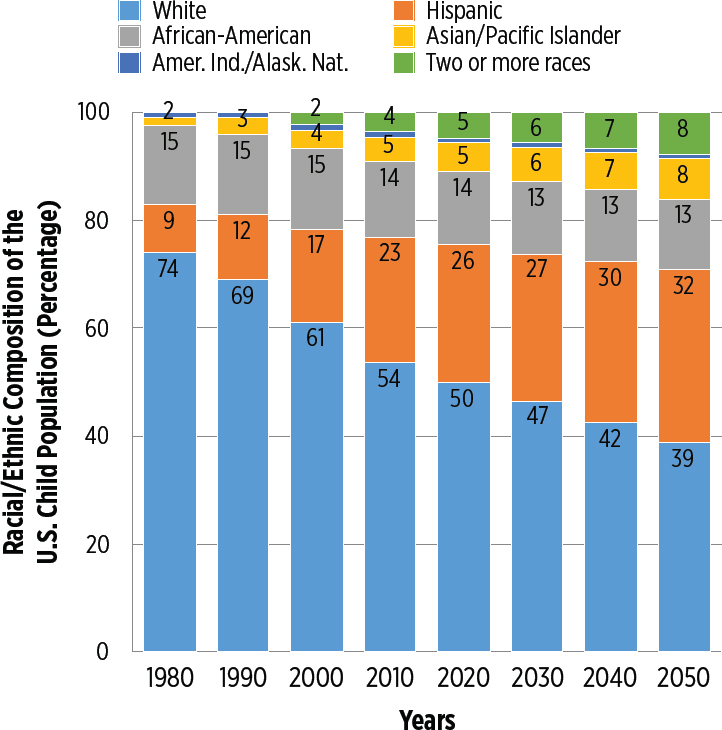
NOTES: Racial groups include only non-Hispanic members. Hispanics may be of any race. Data on two or more races not available before 2000. These data are available on the U.S. Census Bureau website on the Population Estimates and Population Projections pages. The data for 1980 to 2009 are intercensal estimates and incorporate the 1980, 1990, 2000, and 2010 Censuses as benchmarks. The data for 2010 to 2016 are based on the population estimates released for July 1, 2016. Data beyond 2016 are derived from the national population projections released in December 2014.
SOURCE: U.S. Census Bureau, Population Division, obtained from Federal Interagency Forum on Child and Family Statistics (2017).
from 6 percent in 1970 to 25 percent in 2016 (Capps and Fortuny, 2006; Federal Interagency Forum on Child and Family Statistics, 2017). Children in immigrant families are more than 25 percent of the child population in 13 states and in 31 of the 100 largest metropolitan areas (Urban Institute, 2018). Child poverty in families where parents are U.S.-born is 9.9 percent, compared with 20.9 percent in families where at least one of the parents is an immigrant (i.e., foreign-born) (refer to Table D2-5). Child poverty is even higher in households where some members are not citizens or are authorized (refer to Table D2-5).
The increasing diversity of the child population—driven largely by the growth in the Hispanic child population—coupled with higher poverty rates among Hispanic, Black, and AIAN children has led to significant changes in the composition of the child population in poverty. As shown in Figures D2-2 and D2-3, the increasing diversity of children in poverty is apparent in both OPM-based and SPM-based figures. In 2016, 33 percent of the poor child population (<100 percent SPM) was White, down from 55 percent in 1970, while in 2016 Hispanic children represented 40 percent of the population of children in poverty, up from 12 percent in 1970. Hispanic children have been the largest group of children in poverty (4.6
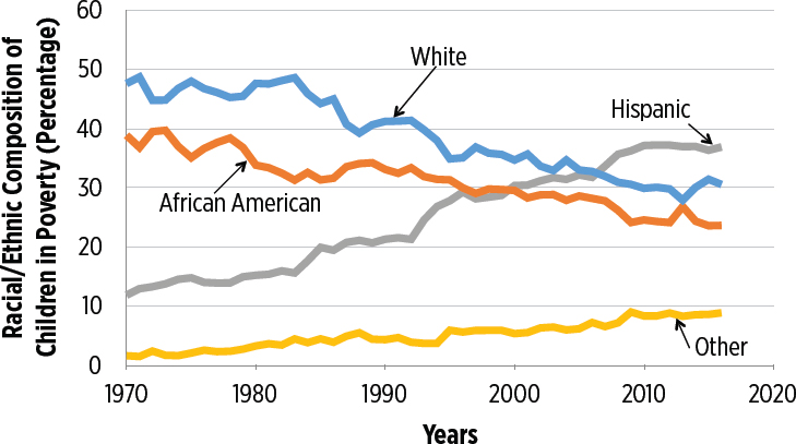
NOTES: Racial groups include only non-Hispanic members. Hispanics may be of any race. Official rates are calculated using the University of Minnesota’s Integrated Public Use Microdata Series (IPUMS.org).
SOURCE: Original analyses commissioned from Sophie Collyer and Christopher Wimer, Columbia Center on Poverty and Social Policy (2018, July).
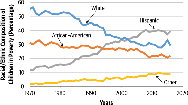
NOTES: The SPM poverty measure is anchored in 2012 living standards and adjusted back to 1967 using the Consumer Price Index. Income data are not adjusted for underreporting. Racial groups include only non-Hispanic members. Hispanics may be of any race.
SOURCE: Original analyses commissioned from Sophie Collyer and Christopher Wimer, Columbia Center on Poverty and Social Policy (2018, July) based on augmented Current Population Survey microdata.
million in 2016) since 2002, followed by White children (3.4 million) and Black children (2.5 million). The trends in the composition of children in poverty based on the OPM are similar to those discussed above based on the SPM, although based on the OPM measure Hispanic children overtook White children to become the largest group in poverty in 2007, 5 years later than they did following the SPM measure.
The downward trend in child poverty for all groups, as measured in SPM-based rates, is readily apparent in Figure D2-4. Because the decline was steeper for minorities, racial/ethnic gaps in child poverty also declined during this period. Between 1970 and 2016, the absolute difference in poverty rates between Black children and White children declined from 38 to 16 percentage points, and between Hispanic and White children from 32 to 16 percentage points. In contrast, gaps in OPM-based poverty rates declined by only about 6 percentage points between Black and White children and remained constant, at about 20 percentage points, between Hispanic and white children (Figure D2-5). The difference between trends
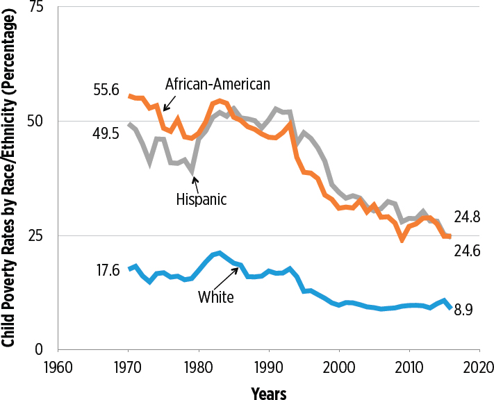
NOTES: The SPM poverty measure is anchored in 2012 living standards and adjusted back to 1967 using the Consumer Price Index. Income data are not adjusted for underreporting. Racial groups include only non-Hispanic members. Hispanics may be of any race.
SOURCE: Original analyses commissioned from Sophie Collyer and Christopher Wimer, Columbia Center on Poverty and Social Policy (2018, July) based on augmented Current Population Survey microdata.
in racial/ethnic gaps computed using SPM and OPM reflects the growth of in-kind transfers to the poorest families, who were disproportionately minority.
Additionally, family structure has changed dramatically in recent decades and, as shown in Figure D2-6, poverty rates have declined for each group—single parent, cohabitating parents, and married parents. TRIM3-adjusted poverty rates for select demographic groups (defined by age of child, region, metropolitan/nonmetropolitan status, disability, and health insurance status) for 2015 are shown in Table D2-6, for deep poverty, poverty, and near poverty.
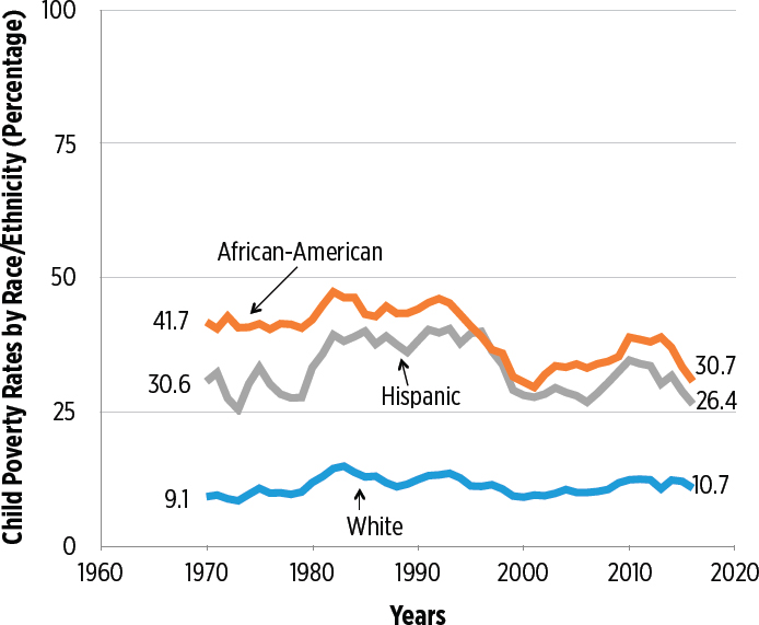
NOTES: Racial groups include only non-Hispanic members. Hispanics may be of any race.
SOURCE: Original analyses commissioned from Sophie Collyer and Christopher Wimer, Columbia Center on Poverty and Social Policy (2018, July). Official rates are calculated using the University of Minnesota’s Integrated Public Use Microdata Series Flood et al. (2017).
APPENDIX D, 2-9
DISTRIBUTION OF CHILD POPULATION ACROSS PERSISTENTLY HIGH-POVERTY COUNTIES
Child poverty rates vary greatly not only by child demographic characteristics but also geographically. The material hardships associated with poverty and families’ ability to get out of poverty vary across communities. The experience of child poverty in a community with good schools and resources for families and with pathways for economic mobility may be different than in a community that has suffered persistent poverty for decades. The burden of poverty may be harder in rural areas where access to services for low-income families may be limited (Schaefer, Mattingly, and Johnson, 2016).
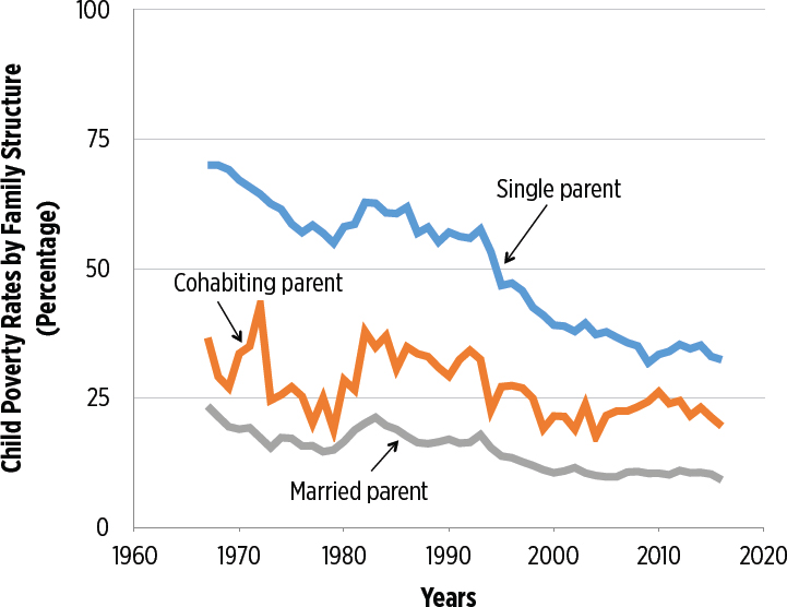
SOURCE: Original analyses commissioned by the committee from Christopher Wimer (2017, October).
As discussed in Chapter 2, we classified a county as experiencing persistently high poverty if 20 percent or more of children under 18 years old were poor as measured by the 1980, 1990, and 2000 decennial censuses and the American Community Survey’s 5-year estimates for 2007–2011.32 Using this definition, we classified 708 of 3,141 counties in the United States as persistently high-poverty counties. The analyses use county-level estimates of the U.S. child population by race/ethnicity provided by the Census Bureau as part of the U.S. Population Estimates Program (data are as of July 1, 2015). In analyses by race/ethnicity, Hispanics may be of any race; other racial groups exclude Hispanics.
In the following, we analyze the distribution of the child population across persistently poor and nonpoor counties, focusing on disparities between racial/ethnic groups, metropolitan and nonmetropolitan areas, and states. We then repeated the analysis using point-in-time poverty rates
___________________
32 This definition was adapted from the U.S. Department of Agriculture. For more information, see https://www.ers.usda.gov/webdocs/DataFiles/48652/ERSCountyTypology2015Edition.xls.
to classify counties as poor versus nonpoor. Specifically, we used the 2015 poverty rate for children under 18 from the Census Small Area Income and Poverty Estimates (SAIPE) Program to classify counties as poor if 20 percent or more children under 18 years old were poor in 2015. Using this definition, we classified 1,858 of 3,141 counties as poor counties. By this definition, more than one-half of all counties are currently poor. We refer to either persistently poor counties or point-in-time poor counties to distinguish between the two definitions.33
Approximately 10 million children ages 0 to 17 resided in persistently poor counties in 2015 (Table D2-7). This corresponds to 13.9 percent of the 74 million children under age 18 living in the United States. Of children living in persistently poor counties, 73 percent resided in metro areas, while 27 percent resided in nonmetro areas (Table D2-6). There are significant racial/ethnic differences in the proportion of children who live in persistently poor counties: from 8.2 percent of Asian and Pacific Islander children to 36 percent of AIAN children (Figure D2-7). In all racial/ethnic groups, except for AIAN children, the majority of children in persistently poor counties live in metropolitan areas (Figure D2-8). However, children in persistently poor counties are more likely to live outside metropolitan areas (26.7%) than children in nonpersistently poor counties (11.9%) (Table D2-8). As discussed in greater detail later in this appendix, most children in persistently poor counties live in the South (6.2 million, 61.1 percent, see Table D2-11). In absolute terms, (non-Hispanic) White children represent the largest racial/ethnic group of children living in persistently poor counties (Table D2-8). However, compared to the 3.6 million White children living in persistently poor counties, the number of Hispanic and (non-Hispanic) Black children living in such counties is of similar magnitude, 3.1 million and 2.7 million, respectively.
Among White children residing in persistently poor counties, 61 percent live in metro areas (Figure D2-8). The comparable figures for Black, Hispanic, and AIAN children are 77.7 percent, 85.4 percent, and 22.6 percent, respectively. In nonmetro area counties that are persistently poor, 51 percent of children are White, 22.4 percent are Black, and 16.6 percent are Hispanic (Figure D2-9). In metro-area counties that are persistently poor, each of these groups contributes about 30 percent of the child population (Figure D2-9).
In contrast, 66 percent of children living in currently poor metro counties are White, 12.1 are Black, and 13.8 are Hispanic (Figure D2-10). In
___________________
33 We also repeated parts of the analysis using the 2015 poverty rate of the total population to classify counties as poor vs. nonpoor. In this case, counties were classified as poor if 20 percent or more of the total county population was poor. Using this classification, 755 of 3,414 counties were classified as poor.
TABLE D2-6 Percent of Children in Poverty based on TRIM3—Adjusted SPM for 2015 by Level of Poverty
| <50 percent SPM (deep poverty) | <100 percent SPM (SPM poverty rate) | 100-149 percent SPM (near poverty) | |
|---|---|---|---|
| All Children | 2.9 | 13.0 | 22.6 |
| Age of Child | |||
| 0–5 Years | 3.1 | 13.9 | 23.8 |
| 6–17 Years | 2.8 | 12.6 | 22.0 |
| Race/Ethnicity | |||
| White-only (non-Hispanic) | 2.1 | 7.9 | 15.0 |
| Black-only (non-Hispanic) | 3.7 | 17.8 | 32.8 |
| Hispanic | 4.0 | 21.7 | 32.9 |
| Other (non-Hispanic)a | 3.3 | 11.1 | 22.0 |
| Metro Status b | |||
| Principal City of Metro Area | 3.3 | 16.9 | 27.4 |
| Metro Area, Not Principal City | 2.9 | 11.8 | 20.7 |
| Metro Area, Principal City Status Not Disclosed | 3.1 | 11.1 | 21.7 |
| Nonmetro Area | 3.0 | 11.1 | 20.3 |
| Region | |||
| Northeast | 2.8 | 12.8 | 21.4 |
| South | 3.4 | 14.4 | 23.3 |
| Midwest | 2.1 | 9.6 | 19.4 |
| West | 2.8 | 14.0 | 25.0 |
| Nativity of Parent/Head | |||
| Native-born Parent/Head | 2.2 | 9.9 | 20.8 |
| Immigrant Parent/Head | 3.8 | 20.9 | 27.7 |
| Citizenship/Legal Status of Childc, d | |||
| All Unit Members Are Citizens | 2.3 | 10.2 | 20.4 |
| Child is a Citizen, Unit Contains Unauthorized Immigrant | 6.4 | 31.5 | 32.7 |
| Child is a Citizen, Unit Contains Recent Immigrant | 3.4 | 24.7 | 27.0 |
| Child is a Citizen, Unit Contains Other Immigrant | 2.4 | 17.7 | 33.7 |
| <50 percent SPM (deep poverty) | <100 percent SPM (SPM poverty rate) | 100-149 percent SPM (near poverty) | |
|---|---|---|---|
| Child is a Noncitizen, Unit Contains Unauthorized Immigrant | 15.2 | 33.3 | 26.5 |
| Child is a Noncitizen, Unit Contains Recent Immigrant | 7.3 | 31.8 | 32.3 |
| Child is a Noncitizen, Unit Contains Other Immigrant | 4.7 | 22.5 | 40.6 |
| Family Composition | |||
| Married/Cohabitating Parents | 1.9 | 9.3 | 18.2 |
| Single Parent | 5.0 | 22.4 | 35.5 |
| No Parents | 7.6 | 22.9 | 24.3 |
| Employment/Health Status of Adults in Unite, f | |||
| 1+ Full-year/Full-time Worker | 0.9 | 6.5 | 19.6 |
| 1+ Part-year or Part-time Worker | 5.5 | 27.8 | 36.1 |
| No Workers, 1+ Adult Neither Elderly or Disabled | 27.9 | 69.1 | 23.8 |
| No Workers, All Adults Elderly or Disabled | 7.3 | 45.4 | 40.0 |
| No Adults in Unit | 81.5 | 90.3 | 5.1 |
| Education of Biological Mother, Father, or Unit Head | |||
| No HS Degree/No GED | 6.5 | 32.5 | 38.2 |
| HS degree/GED, No College | 3.4 | 17.7 | 30.9 |
| Some College, No BA | 2.0 | 9.9 | 25.1 |
| BA+ | 1.5 | 4.8 | 8.8 |
| Age of Mother, Father, or Unit Headg | |||
| Under 25 Years | 5.7 | 23.8 | 36.0 |
| 25 to 35 Years | 3.2 | 14.4 | 28.1 |
| 35+ Years | 2.3 | 11.4 | 19.0 |
| Child’s Health Insurance | |||
| Has Private | 2.0 | 7.0 | 14.2 |
| Has Public | 4.0 | 23.3 | 37.7 |
| Uninsured | 6.3 | 20.2 | 27.6 |
a The Other (Non-Hispanic) race/ethnicity category includes children who are Asian or Pacific Islanders or American Indian or Alaska Natives, or who report more than one race.
b The Metro status category categorizes a child’s household by geography. A metropolitan area includes a large population nucleus and any outlying communities that are highly socially or economically integrated with the nucleus. Nonmetropolitan areas are those outside of metropolitan areas. Households in the Principal city of metro area category live within the largest city of the metropolitan area, and Metro area, nonprincipal city captures households in communities adjacent to the largest city. Some households do not have their metro status suppressed to preserve privacy, and are captured in the Metro Area, principal city status not disclosed category. For more information on this category, see the Current Population Survey Subject Definitions, available at https://www.census.gov/programs-surveys/cps/technicaldocumentation/subject-definitions.html.
c If a child has at least one biological, adoptive, or step-parent that was born in another country, the child is classified as having an immigrant parent. Persons born abroad to American parents are counted as native-born. If a child does not have a parent present, the immigrant status of the unit head and the unit head’s spouse are used, unless the child is the unit head, spouse, or cohabiting partner (these children are tabulated separately).
d The child is placed in the first row that applies. Citizens include both native-born and naturalized citizens. An Other noncitizen includes noncitizens not classified as unauthorized, recent, or temporary. These include legal permanent residents who have been in the United States for more than 5 years and refugees/asylees.
e These rows reflect the work status of persons aged 18 or older in the unit. Full-year is classified as 50 weeks or more, and full-time is classified as 35 hours per week or more.
f A child is classified as being in a unit with a person with a disability if there is at least one person in the unit who is younger than 65 and is identified as disabled according to the definition used when determining SSI eligibility.
g These rows reflect the characteristics of the biological, adoptive, or stepmother (if present), otherwise the biological, adoptive, or stepfather (if present). If neither the father nor mother is present, then the characteristics of the SPM unit head are used, unless the child is the unit head, spouse, or cohabiting partner.
SOURCE: TRIM3 analyses commissioned by the committee.
TABLE D2-7 Distribution of Children Under 18 Across Persistently Poor and Nonpoor Counties, by County Metro Area Status
| Nonpoor | Poor | Total | |
|---|---|---|---|
| Nonmetro | 7,542,121 (11.9%) |
2,726,995 (26.7%) |
10,269,116 (13.9%) |
| Metro | 55,850,927 (88.1%) |
7,496,716 (73.3%) |
63,347,643 (86.1%) |
| Total | 63,393,048 (100%) |
10,223,711 (100%) |
73,616,759 (100%) |
SOURCE: U.S. Population Estimates, 2016 Vintage, Census Bureau. Data as of July 1, 2015.
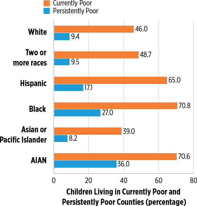
SOURCES: U.S. Population Estimates, 2016 Vintage, Census Bureau. Data as of July 1, 2015; U.S. Population Estimates, 2016 Vintage, Census Bureau. Data as of July 1, 2015. 2015 county poverty rates from Census Small Area Income and Poverty Estimates (SAIPE) Program data.
currently poor non-metro counties, those groups make up 39.1, 19.3, and 33.1 percent of the child population, respectively (Figure D2-10). At 39.8 million, the number of children residing in point-in-time poor counties in 2015 was considerably larger than the number in persistently poor counties, which is not surprising given the much larger number of counties that are poor at a point in time (Table D2-8). Persistent poverty is more prevalent outside of metropolitan areas than point-in-time poverty. While 27 percent of children residing in persistently poor counties live outside a metro area, only 18 percent of children residing in currently poor counties do (Tables D2-7 and D2-8).
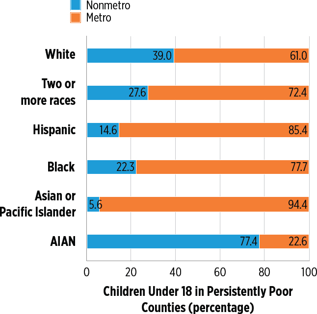
SOURCE: U.S. Population Estimates, 2016 Vintage, Census Bureau. Data as of July 1, 2015.
The racial/ethnic composition of children living in persistently poor counties differs from that of children living in point-in-time poor counties (see Tables D2-9 and D2-10). While white children accounted for 35 percent of children living in persistently poor counties, they make up 44 percent of poor children in point-in-time poor counties (Tables D2-8 and D2-9). Relative to the total number of children of a given race/ethnicity, the risk of residing in a point-in-time poor county is highest among Black children (70.8%), followed by AIAN (70.6%), Hispanic (65.0%), and (non-Hispanic) White children (46.0%) (Figure D2-7).
The percentage of children under 18 living in persistently poor counties varies across U.S. regions. In the South, 22.1 percent of children live in persistently poor counties. In the Northeast, the corresponding figure is 17.3 percent (Figure D2-11). Together, the South and Northeast account
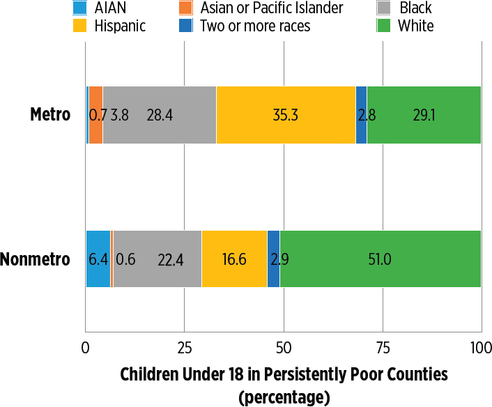
SOURCE: U.S. Population Estimates, 2016 Vintage, Census Bureau. Data as of July 1, 2015.
for most of the child population living in persistently poor counties (Table D2-11). Of the 10.2 million children living in persistently poor countries, 81.2 percent reside in the Northeast and South (Table D2-11). In 10 states and the District of Columbia, more than a quarter of the child population lives in persistently poor counties (Figure D2-13). In Mississippi, nearly two-thirds of the child population live in persistently poor counties. In Alabama, Louisiana, and New Mexico, more than 40 percent of the child population live in persistently poor counties (Figure D2-12).
While there are a large number of White children living in persistently poor counties across the United States (Figures D2-12 and D2-13), AIAN, Black and especially Hispanic children residing in persistently poor counties are more geographically concentrated. Black children in persistently poor counties reside in certain states in the South and Northeast, especially Alabama, Georgia, Louisiana, Mississippi, and New York. Hispanic children in persistently poor counties reside especially in California, New York, and
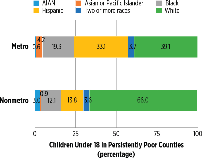
SOURCES: U.S. Population Estimates, 2016 Vintage, Census Bureau. Data as of July 1, 2015. 2015 county poverty rates from Census Small Area Income and Poverty Estimates (SAIPE) Program data.
TABLE D2-8 Distribution of Children Under 18 Across Point-in-Time Poor and Nonpoor Counties, by County Metro Area Status
| Nonpoor | Poor | Total | |
|---|---|---|---|
| Nonmetro | 3,230,445 (9.6%) |
7,038,671 (17.7%) |
10,269,116 (13.9%) |
| Metro | 30,564,379 (90.4%) |
32,783,264 (82.3%) |
63,347,643 (86.1%) |
| Total | 33,794,824 (100%) |
39,821,935 (100%) |
73,616,759 (100%) |
SOURCES: U.S. Population Estimates, 2016 Vintage, Census Bureau. Data as of July 1, 2015. 2015 county poverty rates from Census Small Area Income and Poverty Estimates (SAIPE) Program data.
TABLE S2-9 Distribution of Children Under 18 Across Persistently Poor and Nonpoor Counties, by Race and Ethnicity
| Nonpoor | Poor | Total | |
|---|---|---|---|
| American Indian and Alaska Native | 402,969 | 226,752 | 629,721 |
| Asian or Pacific Islander | 3,404,450 | 302,707 | 3,707,157 |
| Black | 7,416,904 | 2,739,431 | 10,156,335 |
| Hispanic | 15,060,545 | 3,096,243 | 18,156,788 |
| Two or More Races | 2,748,639 | 290,052 | 3,038,691 |
| White | 34,359,541 | 3,568,526 | 37,928,068 |
| Total | 63,393,048 | 10,223,711 | 73,616,759 |
SOURCE: U.S. Population Estimates, 2016 Vintage, Census Bureau. Data as of July 1, 2015. Hispanics may be of any race. Other racial groups exclude Hispanics.
TABLE D2-10 Distribution of Children Under 18 Across Point-in-Time Poor and Nonpoor Counties, by Race and Ethnicity
| Nonpoor | Poor | Total | |
|---|---|---|---|
| American Indian and Alaska Native | 185,122 | 444,599 | 629,721 |
| Asian or Pacific Islander | 2,261,132 | 1,446,025 | 3,707,157 |
| Black | 2,963,092 | 7,193,243 | 10,156,335 |
| Hispanic | 6,350,141 | 11,806,647 | 18,156,788 |
| Two or More Races | 1,559,633 | 1,479,058 | 3,038,691 |
| White | 20,475,704 | 17,452,363 | 37,928,068 |
| Total | 33,794,824 | 39,821,935 | 73,616,760 |
SOURCES: U.S. Population Estimates, 2016 Vintage, Census Bureau. Data as of July 1, 2015. 2015 county poverty rates from Census Small Area Income and Poverty Estimates (SAIPE) Program data.
Texas, which jointly account for 70 percent of Hispanic children living in persistently poor counties; Texas alone accounts for 43.5 percent. Arizona, New Mexico, North Carolina, and Oklahoma account for 60 percent of Native American children living in persistently poor counties.
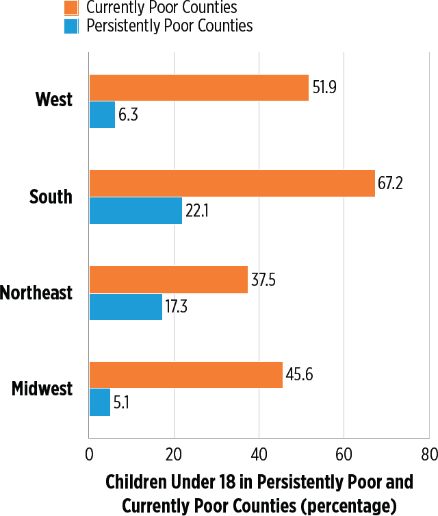
SOURCES: U.S. Population Estimates, 2016 Vintage, Census Bureau; U.S. Population Estimates, 2016 Vintage, Census Bureau. Data as of July 1, 2015. 2015 county poverty rates from Census Small Area Income and Poverty Estimates (SAIPE) Program data.
TABLE D2-11 Child Population Living in Persistently Poor and Currently Poor Counties, by Region
| Number of Children (Millions) | Percentage of Children | |
|---|---|---|
| Persistently Poor Counties | ||
| Midwest | 0.8 | 7.7 |
| South | 6.2 | 61.1 |
| Northeast | 2.1 | 20.2 |
| West | 1.1 | 11.0 |
| Point-in-time Poor Counties | ||
| Midwest | 7.1 | 17.9 |
| South | 19.0 | 47.7 |
| Northeast | 4.5 | 11.2 |
| West | 9.3 | 23.2 |
SOURCES: U.S. Population Estimates, 2016 Vintage, Census Bureau. Data as of July 1, 2015. 2015 county poverty rates from Census Small Area Income and Poverty Estimates (SAIPE) Program data.
APPENDIX D, 2-10
ANCHORED AND UNANCHORED METHODS OF CALCULATING SPM POVERTY OVER TIME
Changes in poverty measured using the SPM could be in part due to changes in poverty thresholds. The SPM was designed to be a relative measure of poverty with poverty thresholds increasing over time as living standards at the 33rd percentile of the American income distribution increased. Some observers such as Wimer et al. (2013, 2016) and Fox et al. (2015) have suggested that an anchored measure may be more useful for measuring poverty over time because it applies a single threshold over the entire time period. An anchored measure of poverty does not take into account changes in living standards when assessing changes in poverty over time (Wimer et al., 2013). Rather, it uses a fixed benchmark for living standards, making it arguably more useful for establishing how the amount of families’ resources has changed over time. Like the OPM, the anchored SPM is an absolute measure of poverty. (Also see discussion of absolute versus relative poverty measures in Appendix D, 2-2.)
The anchored SPM used in the text backdates and updates the poverty threshold from 2012 to reflect today’s consumption norms while adjusting only for inflation. The result is an absolute poverty measure that shows poverty trends over time in relation to contemporary consumption patterns and inflation. Figure D2-15 shows the difference in trends between the anchored and unanchored or absolute and relative SPM measures.
The relative, unanchored SPM shows less progress against child poverty than the absolute, anchored SPM poverty measure. This is because
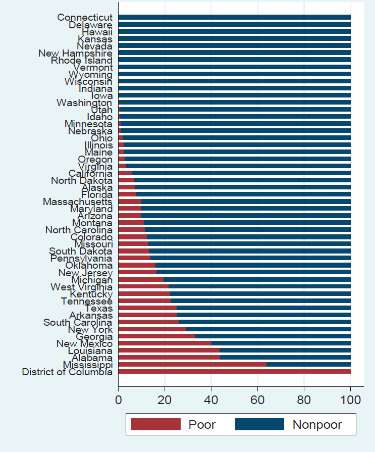
SOURCE: U.S. Population Estimates, 2016 Vintage, Census Bureau. Data as of July 1, 2015.
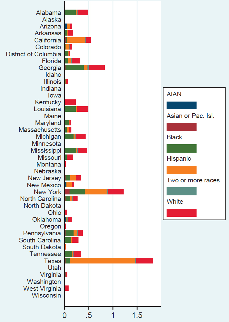
SOURCE: U.S. Population Estimates, 2016 Vintage, Census Bureau. Data as of July 1, 2015.
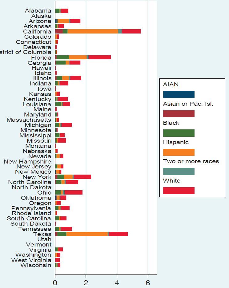
SOURCES: U.S. Population Estimates, 2016 Vintage, Census Bureau. Data as of July 1, 2015. 2015 county poverty rates from Census Small Area Income and Poverty Estimates (SAIPE) Program data.
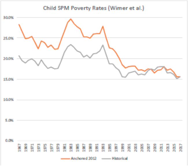
SOURCE: Wimer et al. (2013).
living standards at the 33rd percentile of the income distribution increased somewhat more rapidly than inflation. The poorest families with children were better off in an absolute sense—the anchored poverty rate dropped by nearly one-half. But when compared to the progress of lower middle class families—those at the 33rd percentile—the progress of the poorest families is less impressive—only a 25 percent cut in poverty.
As described in the text, the committee chose to focus on the anchored poverty measure because it wished to isolate the effects of income transfers from the effects of changes in living standards. This is especially salient for comparisons of the OPM to the SPM. A comparison of the OPM to unanchored SPM mixes together differences in counting key transfers with differences between an absolute and relative poverty measure. Whether the absolute or relative SPM is a superior measure remains an open question. For further discussion see Wimer et al. (2013, 2016) and Garfinkel, Rainwater, and Smeeding (2010). Future research should address this issue by comparing the two time series with other measures of economic deprivation such as food insecurity and other forms of material hardship.
APPENDIX D, 2-11
POVERTY MEASUREMENT ACROSS COUNTRIES: CROSS-COUNTRY POVERTY LINES AND CHILD POVERTY RATES
To understand child poverty in the United States relative to peer nations, the committee commissioned analyses comparing child poverty measures in the United States to four Anglophone nations: Australia, Canada, Ireland, and the United Kingdom. Data from the Luxembourg Income Study (LIS) and the Organisation for Economic Co-operation and Development (OECD) poverty and income database were used to compare child poverty across the five nations. The results of these analyses are discussed in Chapter 2.
The common international standards and measurement methods for poverty statistics are different from those of the SPM measure in several ways. For this reason, comparisons of poverty across countries are problematic. Both LIS and OECD calculate poverty based on disposable income. The SPM definition of disposable income largely follows the LIS and OECD but differs in a number of ways. Specifically, it
- subtracts medical out-of-pocket expenses and work-related costs;
- adjusts for cost-of-living differences within the nation;
- separates poverty lines for owners with and without mortgage and renters; and
- uses cohabiter units and families who meet income-sharing rules, not households.
The SPM also takes a different approach to equivalence scales. Poverty measurement typically adjusts income for family size using an equivalence scale (as described in Appendix D, 2-1), reflecting a less-than-proportional increase in expenses as the number of family members increases. For example, considering the resource needs of a family with a given number of children, one can express the spectrum of possible adjustments through the exponent X in the following simple equation:
Needs = (Number of children)X
where X = 1 in the case of equal needs for all family members and X = 0 if needs do not increase at all with increases in family size. As detailed in Appendix D, 2-1, the SPM sets X at 0.7 for families with children, which effectively assumes that having two children generates the need for an income that is 62 percent greater than having one child, and that having three children generates 2.2 times the need of one. The equivalence scale in the LIS sets X at 0.5, which differs from both the OECD scale and the
SPM scale. Finally, the LIS and OECD statistics do not include adjustments for underreporting for benefits or other income sources.
Cross-Country Relative Poverty
Figure 2-13 (in the body of Chapter 2) first presents child poverty rates using the OECD-50 for the United States and the four anglophone comparison countries in 2015. This poverty measure indicates that the child is poor if the equivalized income is less than one-half of the median. The United States is the clear outlier in terms of relative poverty rates: 19.9 percent of children in the United States are classified as poor compared to 15 percent in Canada, 13 percent in Australia, and less than 12 percent in the United Kingdom and Ireland according to OECD-50. The qualitative results compare well with similar measures from LIS (see LIS-50 in Figure D2-16) as well as the existing literature (e.g., Smeeding and Thevenot, 2016; Gornick and Nell, 2017).
To understand differences in child poverty across countries with an SPM-type poverty threshold, the committee attempted to adjust the SPM to the international standards. To construct an SPM-based relative poverty measure, we took the four-person U.S. SPM poverty threshold and compared it to the median income for a family of four in the United States in the LIS. Ignoring health care costs and work expenses and other adjustments, the SPM poverty line cuts the LIS U.S. income distribution at the 40th percentile. Based on this, we then define relative poverty lines across all five countries at the 40th percentile of their respective income distributions. The resulting child poverty rates, shown as LIS-SPM-40 in Figure 2-13 in Chapter 2 and Figure D2-16, produce a country ordering similar to that based on the OECD poverty measures, with U.S. poverty rates (12.3%) much higher than those in all other countries, including the second- highest ranked, Canada (10.1%).
Cross-Country Absolute Poverty
In addition to relative poverty comparisons, it is also useful to compare countries based on absolute poverty differences. It is not possible to implement all of the SPM adjustments in LIS data, nor can the OECD data be changed to accommodate an absolute poverty line. Instead, the committee adjusted the SPM to be comparable to the LIS. Building on the analysis above, the SPM poverty line, ignoring health care costs, work expenses and other adjustments for COLAs and housing status, is about 40 to 41 percent of U.S. median adjusted income (Short, 2013; Wimer and Smeeding, 2017). The committee used these and set the poverty line for two adults and two children as $25,551, which was 40.2 percent of LIS median household
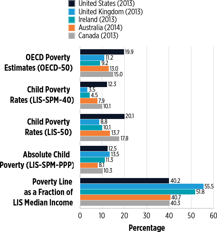
SOURCE: Original LIS analyses commissioned by the committee from the LIS Cross-National Data Center.
income (bottom panel of Figure D2-16). The LIS team converted this line to other nations’ incomes using purchasing power parities (PPPs) and national price indices where years differ (Gornick and Jantti, 2013; Gornick and Nell, 2017; Rainwater and Smeeding, 2003).34
Using these PPP-adjusted poverty thresholds, we can compare child poverty rates in the five countries in terms of absolute poverty; this is shown in Figure D2-16 and labeled LIS-SPM-PPP. Reflecting higher average income in the United States compared to our peer English-speaking nations, using an absolute poverty line across countries rather than a relative poverty line within each country leads to a different cross-country ranking. In particular, as shown in the bottom panel of Figure D2-16, the absolute poverty line is about 40 percent of median income in the United States, Canada, and Australia, but it is 52 percent of median income in Ireland and almost 56 percent of median income in the United Kingdom. The resulting absolute child poverty rates (fourth panel of Figure D2-16, LIS-SPM-PPP) are highest in the United Kingdom (13.5%), followed by the United States (12.5%), Ireland (11.3%), and Canada (10.3%)—and are quite a bit lower in Australia (8.1%).
We see where the LIS-SPM-PPP poverty line cuts the distributions in other nations at the bottom of Figure D2-16. In contrast, we could take the official U.S. poverty line used by others to make absolute comparison across nations (Gornick and Nell, 2017) and see where it cuts the other nations’ distributions. The comparison of these approaches for the United States and United Kingdom indicates the sensitivity of absolute poverty measures in an international context. In Figure D2-16 we compare the two absolute poverty lines for a family of four (both in PPP 2013 prices): the $25,551 LIS-SPM-PPP poverty line and the $23,306 U.S. official poverty line.
We converted the lines to adjusted income per adult equivalent to assure the same LIS square-root equivalence scale in both comparisons (Figure D2-17). This resulted in equalized poverty lines of $12,348 per equivalent adult for the SPM PPP line and $11,518 per equivalent adult for the U.S. official line. These lines are drawn vertically and compared to the cumulative distributions of real PPP adjusted income per equivalent adult for families with children in the United States (blue) and the United Kingdom (orange). At the U.S. official line, child poverty is slightly higher in the United States, at 10.5 percent, than in the United Kingdom, at 10.0 percent. But at the SPM line, the opposite is true: the U.S. child poverty
___________________
34 The 2013 U.S. SPM translates into about $25,550 for two parents and two children. These are converted to other currencies first using 2011 PPP and then using national consumer price changes when the LIS years differ from 2013. See Pinkoyskiy and Sala-i-Martin (2018) for more information about using PPPs.
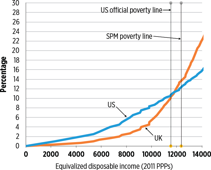
SOURCE: Original LIS analyses commissioned by the committee from the LIS Cross-National Data Center.
rate of 12.5 percent is below the UK child poverty rate of 13.5 percent, as shown in Figure 2-13 in Chapter 2 and Figure D2-16.35
Using these LIS-based absolute poverty measures, we can extend this analysis to make a fuller comparison of poverty rates for the United States and the four comparison countries. Figure D2-18 compares absolute poverty at the deep poverty line (one-half the U.S. SPM-PPP line in absolute terms) and near poverty (using 150% of the U.S. SPM-PPP poverty line). As the figure shows, the highest rates of absolute deep poverty are in the United States (3.6%, far above the next highest, which is in Australia at 1.9%) but the highest rates of near-poverty are found in the United Kingdom (46.4%).
Figure D2-19 shows the absolute child poverty rates among single-parent families, families with one or more full-time worker, and immigrant
___________________
35 These results are comparable to those found in Gornick and Nell (2017), who used 2011 data to make the same calculations.
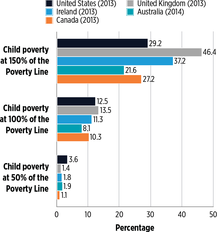
SOURCE: Original LIS analyses commissioned by the committee from the LIS Cross-National Data Center.
families using the same absolute measure (LIS-SPM-PPP). Children in single-parent families are considerably poorer in the United States (30.6%) than in other nations in absolute poverty terms, even comparing the United Kingdom with its lower living standards as well as Australia (19.1%) and Canada (26.3%) with similar living standards. In contrast, child poverty rates in two-parent families are only 6.4 percent in the United States. Only Australia has a lower rate, at 5.9 percent (not shown here). But the low-wage United States has the second highest absolute poverty rate for children in families with at least one full-time worker, 7.0 percent, with only
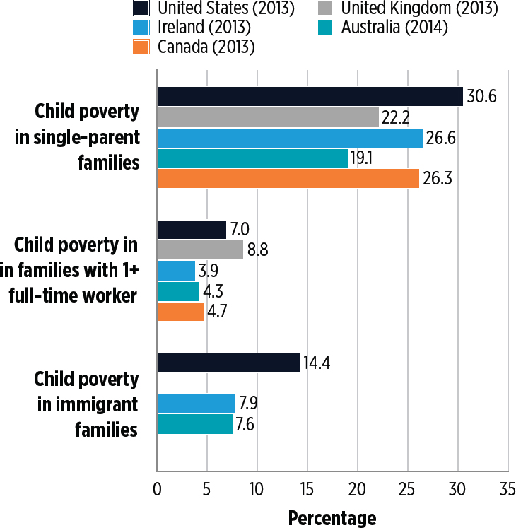
NOTE: A family in which any adult is an immigrant (based on citizenship and country of origin) is categorized as an immigrant family.
SOURCE: Original LIS analyses commissioned by the committee from the LIS Cross-National Data Center.
the United Kingdom higher, at 8.8 percent, while all the other nations fall below 4 percent (Figure D2-19).
Another important dimension to compare across countries is with respect to immigrant status (bottom panel of Figure D2-19). However, in the LIS, comparable data on immigrant status is available only for Australia
and Ireland.36 In these two countries, absolute immigrant child poverty rates are below 8 percent, compared to 14.4 percent in the United States. Finally, the LIS estimated absolute child poverty excluding non-Hispanic Blacks in the United States, lowering the U.S. absolute poverty rate from 12.5 to 10.3 percent. Racial differences therefore make an almost 20 percent difference in the U.S. poverty rate compared to other English-speaking rich nations without a significant racial minority.
Cross-Country Comparisons of Income
Given the differences in country rankings of absolute and relative poverty measures, we conclude this appendix with a discussion of disposable household income and other real income concepts to get a better understanding of living standards across the five English-speaking nations of interest. In the LIS results, different equivalence scales, different years and different PPPs may all produce different results in terms of median incomes. Further, there is underreporting in all household income surveys. These are corrected for in the TRIM3 simulations, but not in LIS or OECD surveys.
And so, here we explore differences in living standards across countries by comparing three series of real PPP adjusted income indexes to the United States. These results are shown in Table D2-12. The first column shows the LIS-SPM-PPP poverty lines as a fraction of median incomes, as seen in Figure D2-16. The second column shows ratios of median equivalized income from the LIS database. The third column shows OECD household disposable income per capita (adjusted to National Income and Product Account totals). And the fourth column shows GDP per capita from the International Monetary Fund. For each measure, the four comparison countries are presented relative to the United States (so the value for the United States equals 100 for each).
There are several things to take away from this table. First, all of the numbers are less than 100 for each of the four comparison countries, indicating that on a range of measures the United States is on average richer than our peer English-speaking countries. Second, across all measures, Australia and Ireland come closest to the U.S. values. Third, the magnitude of the disparities across countries varies significantly across the measures.
Based on the LIS median equivalized income, Australia and Canada are nearly identical to the United States (98.7 for Australia and 99.7 for Canada). However, based on disposable income per capita or GDP per capita, the disparities are much larger. The opposite pattern is present in Ireland, although the Ireland LIS data (from 2010) are probably showing lower incomes due to the Great Recession. Finally, the United Kingdom
___________________
36 The Canadian and UK LIS datasets suppress immigrant status.
TABLE D2-12 Income Comparisons Across Anglophone OECD Countries Using Different Measures of Real Income, Indexed to USA = 100
| SPM Poverty Line as a Fraction of Equivalized LIS Median Income, Using 2011 PPP $ | 2013 LIS Real Median Equivalent Income/US Median Equiv. Income | 2013 OECD Real Disposable Household Income Per Capita/USA Value | 2013 Real GDP Per Capita/USA GDP Per Capita | |
|---|---|---|---|---|
| Australia, 2014 | 40.7 | 98.7 | 82.0 | 86.0 |
| Canada, 2013 | 40.3 | 99.7 | 70.5 | 83.1 |
| Ireland, 2010 | 51.8 | 79.1 | 85.0 | 89.9 |
| United Kingdom, 2013 | 55.5 | 72.4 | 66.1 | 73.8 |
| United States, 2013 | 40.2 | 100.0 | 100.0 | 100.0 |
NOTES: LIS from Figure D2-16; Poverty line as a fraction of equivalized LIS median income, using 2011 PPP and domestic CPI changes to correct year; LIS: by division, Real 2013 LIS ratio of median equalized incomes in each country to USA 2013, using 2011 PPP and domestic CPI changes to correct year.
SOURCES: Analyses commissioned by the committee from the LIS Cross-National Data Center; OECD real NIPA adjusted household income per capita from https://data.oecd.org/hha/household-disposable-income.htm, using 2011 PPP; IMF Real GDP per capita from http://www.imf.org/external/pubs/ft/weo/2017/01/weodata/index.aspx, using 2011 PPP.
has the lowest real income compared to the United States using all three aggregate income measures, as shown in columns two, three, and four of Table D2-12. Hence the SPM poverty line, at 55 percent of LIS median adjusted income in the United Kingdom in the first column, reflects the lower real UK living standards (evident using three different measures).
REFERENCES
Advisory Commission to Study the Consumer Price Index. (1996). Toward a More Accurate Measure of the Cost of Living. Final Report to the Senate Finance Committee. Washington, DC.
Akee, R., and Simeonova, E. (2017). Poverty and Disadvantage among Native American Children: How Common Are They and What Has Been Done to Address Them? Paper commissioned by the Committee on Building an Agenda to Reduce the Number of Children in Poverty by Half in 10 Years.
Attanasio, O.P., and Pistaferri, L. (2016). Consumption inequality. Journal of Economic Perspectives, 30(2), 3–28.
Bee, A., Meyer, B.D., and Sullivan, J.X. (2012). The Validity of Consumption Data: Are the Consumer Expenditure Interview and Diary Surveys Informative? Working Paper No. 18308. Cambridge, MA: National Bureau of Economic Research.
Berndt, E.R. (2006). The Boskin Commission Report after a decade: After-life or requiem? International Productivity Monitor 12: 61–73. Available: http://www.csls.ca/ipm/12/IPM-12-Berndt-e.pdf?q=boskin.
Bitler, M., Hoynes, H., and Kuka, E. (2017). Child poverty, the Great Recession, and the social safety net in the United States. Journal of Policy Analysis and Management 36(3), 358–389.
Bureau of Economic Analysis. (2017). Real Personal Income for States and Metropolitan Areas. Washington, DC. Available: https://www.bea.gov/newsreleases/regional/rpp/rpp_newsrelease.htm.
Capps, R., and Fortuny, K. (2006). Immigration and Child and Family Policy: Paper 3. Washington, DC: The Urban Institute and Child Trends.
Curran, L.B., Wolman, H., Edward, W., and Furdell, K. (2008). Poverty, Programs, and Prices: How Adjusting for Costs of Living Would Affect Federal Benefit Eligibility. Washington, DC: The Brookings Institution. Available: https://www.brookings.edu/wp-content/uploads/2016/06/0317_costofliving_curran.pdf.
Federal Interagency Forum on Child and Family Statistics. (2017). America’s Children: Key National Indicators of Well-Being, 2017. Washington, DC: Government Printing Office.
Fisher, G.M. (1992). The development and history of the poverty thresholds. Social Security Bulletin, 55(4). Washington, DC: Social Security Administration.
Fitzpatrick, K., and Thompson, J.P. (2010). The interaction of metropolitan cost-of-living and the federal Earned Income Tax Credit: One size fits all? National Tax Journal, 63(3), 419–445.
Fox, L. (2018). The Supplemental Poverty Measure: 2017. Washington, DC: U.S. Census Bureau. Available: https://www.census.gov/content/dam/Census/library/publications/2018/demo/p60-265.pdf.
Fox, L., Wimer, C., Garfinkel, I., Kaushal, N., and Waldfogel, J. (2015). Waging war on poverty: Poverty trends using a historical Supplemental Poverty Measure. Journal of Policy Analysis and Management, 34(3), 567–592.
Garfinkel, I., Rainwater, L., Smeeding, T. (2010). Wealth and Welfare States: Is America a Laggard or Leader? New York, NY: Oxford University Press.
Garner, T. (2010). Supplemental Poverty Measure Thresholds: Laying the Foundation. Washington, DC: Bureau of Labor Statistics.
Gornick, J.C., and Jantti, M. (Eds). (2013) Income Inequality: Economic Disparities and the Middle Class in Affluent Countries. Stanford, CA: Stanford University Press.
Gornick, J.C., and Nell, E. (2017). Children, Poverty, and Public Policy: A Cross-National Perspective. LIS Working Paper No. 701. Luxembourg: LIS Cross-National Data Center. Available: http://www.lisdatacenter.org/wps/liswps/701.pdf.
Hausman, J. (2003). Sources of bias and solutions to bias in the Consumer Price Index. Journal of Economic Perspectives 17:23–44.
Hurst, E. (2012). Comment: Winning the war: Poverty from the Great Society to the Great Recession. Washington, DC: The Brookings Institution. Available: https://www.brookings.edu/bpea-articles/winning-the-war-poverty-from-the-great-society-to-the-great-recession.
Interagency Technical Working Group. (2010). Observations from the Interagency Technical Working Group on Developing a Supplemental Poverty Measure. Available: https://www.federalregister.gov/documents/2010/05/26/2010-12628/developing-a-supplementalpoverty-measure.
Johnson, N. (2017). A Comparison of PCE and CPI: Methodological Differences in U.S. Inflation Calculation and their Implications. Paper presented at the 2016 Joint Statistical Meetings of the Bureau of Labor Statistics, Chicago, IL. Available: https://www.bls.gov/osmr/pdf/st170010.pdf.
Martin, J.A., Hamilton, B.E., Osterman, M.J., Driscoll, A.K., and Drake, P. (2018). Births: Final Data for 2016. Hyattsville, MD: National Center for Health Statistics.
Meyer, B.D., and Mittag, N. (2015). Using Linked Survey and Administrative Data to Better Measure Income: Implications for Poverty, Program Effectiveness, and Holes in the Safety Net. Working Paper No. 21676. Cambridge, MA: National Bureau of Economic Research.
Meyer, B.D., and Sullivan, J.X. (2003). Measuring the well-being of the poor using income and consumption. Journal of Human Resources, 38, 1180–1220.
________. (2011). The Material Well-Being of the Poor and Middle Class Since 1980. Working Paper No. 2011-04. Washington, DC: American Enterprise Institute. Available: http://www.aei.org/wp-content/uploads/2011/10/Material-Well-Being-Poor-Middle-Class.pdf.
________. (2012a). Identifying the disadvantaged: Official poverty, consumption poverty, and the new supplemental poverty measure. Journal of Economic Perspectives 26(3), 111–136.
________. (2012b). Winning the War: Poverty from the Great Society to the Great Recession. Washington, DC: The Brookings Institution.
________. (2017). Annual Report on U.S. Consumption Poverty: 2016. Washington, DC: American Enterprise Institute.
________. (2018). Annual Report on U.S. Consumption Poverty: 2017. Washington, DC: American Enterprise Institute.
Meyer, B.D., and Wu, D. (2018). The Poverty Reduction of Social Security and Means Tested Transfers. Working Paper No. 24567. Cambridge, MA: National Bureau of Economic Research.
Meyer, B.D., Mok, W.K.C., and Sullivan, J.X. (2009). The Under-Reporting of Transfers in Household Surveys: Its Nature and Consequences. Working Paper No. 15181. Cambridge, MA: National Bureau of Economic Research.
________. (2015). Household surveys in crisis. Journal of Economic Perspectives, 29(4), 199–226.
Moffitt, R.A., and Scholz, J.K. (2009). Trends in the Level and Distribution of Income. Working Paper No. 15488. Cambridge, MA: National Bureau of Economic Research. Available: http://www.nber.org/papers/w15488.
National Research Council. (1995). Measuring Poverty: A New Approach. Washington, DC: National Academy Press.
________. (2013). Measuring What We Spend: Toward a New Consumer Expenditure Survey. Washington, DC: The National Academies Press.
Norris, T., Vines, P.L., and Hoeffel, E.M. (2012). The American Indian and Alaska Native Population: 2010. 2010 Census Briefs. Washington, DC: U.S. Census Bureau.
Pinkovskiy, M., and Sala-i-Martin, X. (2018). Shining a Light on Purchasing Power Parities. Working Paper No. 24419. Cambridge, MA: National Bureau of Economic Research.
Rainwater, L., and Smeeding, T.M. (2003). Poor Kids in a Rich Country: America’s Children in Comparative Perspective. New York, NY: Russell Sage Foundation.
Renwick, T., Aten, B., Figueroa, E., and Martin, T. (2014). Supplemental Poverty Measure: A Comparison of Geographic Adjustments With Regional Price Parities vs. Median Rents from the American Community Survey. Washington, DC: Bureau of Economic Analysis. Available: https://www.bea.gov/papers/pdf/BEAWP_PovertyMeasure.pdf.
Schaefer, A., Mattingly, M.J., and Johnson, K.M. (2016). Child Poverty Higher and More Persistent in Rural America. Durham, NH: University of New Hampshire, Carsey School of Public Policy. Available: https://scholars.unh.edu/cgi/viewcontent.cgi?referer=&httpsredir=1&article=1265&context=carsey.
Short, K. (2001). Experimental Poverty Measures: 1999. Washington, DC: U.S. Government Printing Office.
Short, K.S. (2013). The Supplemental Poverty Measure: Examining the Incidence and Depth of Poverty in the U.S. Taking Account of Taxes and Transfers in 2012. U.S. Census Bureau: Washington, DC. Available: https://www.census.gov/content/dam/Census/library/working-papers/2013/demo/kshort-sea2013.pdf.
Tax Foundation. (2017). What is the Real Value of $100 in Your State? Washington, DC. Available: https://taxfoundation.org/real-value-100-state-2017.
Tax Policy Center. (2017). EITC Parameters, 1975 to 2017. Washington, DC. Available: https://www.taxpolicycenter.org/statistics/eitc-parameters.
U.S. Department of Agriculture. (2013). Supplemental Nutrition Assistance Program, July 2013. Available: http://www.fns.usda.gov/snap/applicant_recipients/eligibility.htm#employment.
U.S. Census Bureau. (2016). Fertility: 2016 American Community Survey 1-year Estimates. Washington, DC.
________. (2018a). Annual Estimates of the Resident Population by Sex, Age, Race, and Hispanic Origin for the United States and States: April 1, 2010 to July 1, 2017. Washington, DC: U.S. Census Bureau, Population Division.
________. (2018b). Race by Hispanic Origin: Main Projections Series for the United States, 2017-2060 Washington, DC: U.S. Census Bureau, Population Division.
Urban Institute. (2018). Data from the Integrated Public Use Microdata Series Datasets Drawn from the 2014 and 2015 American Community Survey. Washington, DC.
Wheaton, L. (2008). Underreporting of Means-Tested Transfer Programs in the CPS and SIPP. Washington, DC: Urban Institute. Available: https://www.urban.org/research/publication/underreporting-means-tested-transfer-programs-cps-and-sipp.
Wimer, C., and Smeeding, T. (2017). USA child poverty: The impact of the Great Recession. In Y.C.B. Cantillon, S. Handa, and B. Nolan (Eds.), Children of Austerity: The Impact of the Great Recession on Child Poverty in Rich Countries (pp. 297–331). Oxford: Oxford University Press.
Wimer, C., Fox, L., Garfinkel, I., Kaushal, N., and Waldfogel, J. (2013). Trends in Poverty With an Anchored Supplemental Poverty Measure. Columbia University Academic Commons.
________. (2016). Progress on poverty? New estimates of historical trends using an anchored Supplemental Poverty Measure. Demography, 53(4), 1207–1218.
Winship, S. (2016). Poverty After Welfare Reform. New York: Manhattan Institute. Available: https://www.manhattan-institute.org/sites/default/files/R-SW-0816.pdf.
APPENDIX D, 3-1
ASSOCIATIONS BETWEEN POVERTY AND CHILD OUTCOMES
A large literature documents strong and consistent associations between child poverty and a broad range of negative outcomes for child health and well-being. In Chapter 3, the committee elected to focus on studies that estimated a causal relationship between poverty and child outcomes. In this appendix, we try to give a broader overview of some of the correlational literature, in order to show the pervasiveness of the relationship across many different types of outcomes. This appendix section is not intended as an exhaustive review of the literature. The bulk of this review is organized by domains of child outcomes into the following 10 topical sections: (1) family functioning, child maltreatment, domestic violence, and adverse childhood experiences; (2) material hardship; (3) physical health; (4) fetal health and health at birth; (5) brain development; (6) mental health; (7) educational attainment; (8) risky behaviors, crime, and delinquency; (9) the timing of poverty; and (10) severity of poverty. We also touch upon how these factors can contribute to the intergenerational transmission of poverty.
In addition to the narrative overview, we also offer summary tables of the material treated in the text, one for each section. These tables enable readers to quickly scan the findings, or to locate particular studies. This appendix ends with a consideration of the literature about the relationships between child outcomes and the timing and severity of poverty. The literature is also summarized in companion tables.
FAMILY FUNCTIONING, CHILD MALTREATMENT, DOMESTIC VIOLENCE, AND ADVERSE CHILDHOOD EXPERIENCES
A number of studies have linked child poverty to Adverse Childhood Experiences (ACEs) (Anda et al., 2006) (see Table D3-1). ACEs include abuse or neglect, the death of a parent, divorce or separation of parents, domestic violence, neighborhood violence, family mental illness or substance abuse, and incarceration of a family member. Poor and near-poor children are more than twice as likely to have experienced three or more ACEs than their more affluent peers (Anda et al., 2006; Figure D3-1). Experiencing ACEs early in life has been shown to be predictive of long-lasting negative outcomes in adulthood, such as increased risk for cardiovascular disease, obesity, smoking, drug and alcohol abuse, risky sexual behavior, and early mortality (Anda et al., 2006). It is thought that these life events cause high levels of biological stress on the developing brain, as well as on neurological, hormonal, and immune-response systems, leading to lifelong changes (Shonkoff et al., 2012). Moreover, ACEs have a “dose-response”
TABLE D3-1 Adverse Childhood Experiences
| Author and Year | Source of Data | Findings |
|---|---|---|
| Sedlak et al., 2010 | National Incidence Study (Survey data), 2005 to 2006 |
|
| Paxson and Waldfogel, 2003 | National Center for Child Abuse and Neglect, 1990 to 1998 |
|
| Macomber, 2006 | House Committee on Ways and Means, 2004; National Survey of America’s Families, 2002; The National Intimate Partner and Sexual Violence Survey, 1993 to 1998 |
|
| Cancian, Yang, and Slack, 2013 | Child Support Demonstration Evaluation (CSDE); Wisconsin Statewide Automated Child Welfare Information System, 1997 to 1999 |
|
| Anda et al., 2006 | Adverse Childhood Experiences Study, 1995 to 1996 |
|
| Author and Year | Source of Data | Findings |
|---|---|---|
| National Survey of Children’s Health, 2017 | National Survey of Children’s Health, 2011 to 2012 |
|
| Health Resources and Services Administration, 2015 | Adverse childhood experiences data (U.S. Department of Health and Human Services), 2014 |
|
SOURCES: Health Resources and Services Administration, Maternal and Child Health Bureau; and Centers for Disease Control and Prevention, National Center for Health Statistics, National Survey of Children’s Health. Analyzed by the Health Resources and Services Administration’s Maternal and Child Health Bureau. See https://mchb.hrsa.gov/chusa14/special-features/adverse-childhood-experiences.html#sourcef2.
effect, with children who experienced larger numbers of ACEs experiencing worse outcomes (Anda et al., 2006).
More recently, researchers have suggested adding two additional ACEs: chronic economic hardship and being treated unfairly due to race/ethnicity. These nine ACEs have been added to the National Survey of Children’s Health (NSCH), allowing analysis of association of ACEs with poverty. Since poverty is now one of these ACE questions asked of parents, analysis by poverty levels excludes the experience of economic hardship. Analysis of data from the 2011/12 NSCH documents the significant association of ACEs with child poverty. There is a clear income gradient for ACEs, as shown in Figure D3-1 (National Survey of Children’s Health, 2017). We explore two ACEs, child maltreatment and intimate partner violence, below.
Researchers have repeatedly documented the association between poverty and the risk of child maltreatment, especially in cross-sectional studies of the general population. Children in low socioeconomic status (SES) families were five times more likely than those in higher income families to experience maltreatment of any kind, three times more likely to be physically or sexually abused, and seven times more likely to be neglected (Sedlak et al., 2010). In a study looking at the impact of welfare reform, higher poverty rates were associated with significantly more substantiated cases of child
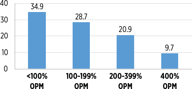
NOTES: Based on the U.S. Department of Health and Human Services poverty guidelines, poverty was $23,050 for a family of four in 2012. OPM = Official Poverty Measure.
SOURCES: Health Resources and Services Administration, Maternal and Child Health Bureau; and Centers for Disease Control and Prevention, National Center for Health Statistics, National Survey of Children’s Health. Analyzed by the Health Resources and Services Administration’s Maternal and Child Health Bureau. See https://mchb.hrsa.gov/chusa14/special-features/adverse-childhood-experiences.html#sourcef2.
maltreatment, cases of physical abuse, and cases of neglect (Paxson and Waldfogel, 2003). Almost one-half of children placed in out-of-home foster care come from homes that are eligible for welfare (Macomber, 2006).
There is some evidence that increasing family income reduces risk of child maltreatment. Cancian and her colleagues (2013) took advantage of the random assignment evaluation of child support during welfare reform in Wisconsin to distinguish the causal effect of income from other causes of child maltreatment. The experimental group received a pass-through of child support and the control group did not. Mothers received additional income, on average, of $81 to $164 per year for 2 years, although some mothers received substantially more. Despite this modest increase in income, children in the experimental group were 10 to 12 percent less likely to have a report of child maltreatment.
Low-income families also experience intimate partner violence at higher rates than other families. For example, women living in households with annual incomes of less than $7,500 are seven times more likely to be victims of domestic violence than those with an income of at least $75,000 (Macomber, 2006). Furthermore, the rate of hospitalizations for domestic assault while pregnant is three times as high for mothers who are on
Medicaid than for those on private insurance (Aizer, 2011). These women are more likely to have poor birth outcomes such as low birth weight infants, fetal death, and increased infant mortality (Aizer, 2011). On average, infants born to mothers hospitalized for assault weigh 163 grams less at birth (Aizer, 2011). The lower birth weights of these infants are likely to lead to poorer heath, lower academic achievement, and reduced income in adulthood, thereby contributing to intergenerational poverty (Almond and Currie, 2011).
The causal relationships between poverty, child maltreatment, and intimate partner violence have been less clear. It is unknown if the higher rates of child maltreatment and domestic violence in low-income families reflect the increased stress of material and economic hardship, preexisting conditions (such as mental illness and substance abuse), the increased contact with mandatory reporters of child maltreatment, or attribution bias among mandatory reporters. For example, the material and economic hardships associated with poverty may lead to increased parenting stress and impact parents’ mental health and family relationships, which, in turn, may lead to violence or maltreatment of the child (for more on this process, see the section on mental health, below). Alternatively, conditions that can lead to poverty and to child maltreatment, such as parental mental health problems and substance abuse, are causing correlations between poverty and child maltreatment that are not causal. Children in low-income families are more likely to have a parent with poor mental health compared with children in higher income families (Macomber, 2006). As is often the case with a physical health problem, mental health problems can detract from the care and attention that a parent can provide their child. And finally, it is possible that the disparities in rates of child maltreatment and intimate partner violence between poor and higher-income families are a product of reporting bias. Poor families are more likely to come into contact with mandated reporters of child maltreatment through their participation in government systems, such as welfare. This increased visibility may lead to greater attention to problems in these families than in families with higher incomes, who are less likely to use welfare and other assistance programs.
MATERIAL HARDSHIP
Material hardship—broadly defined as the inability to meet basic needs—is associated with poverty. Many, but not all, of the negative impacts of poverty on child outcomes may be mediated through those material hardships. Measures of material hardship use indicators of consumption and physical living conditions that are directly related to whether families can meet basic needs, starting with needs for physiological functioning and survival (Ouellette et al., 2004). Therefore, measures of shelter
(housing, utilities), medical care, food security, and ability to pay for essential expenses are always included when researchers measure material hardship. Sometimes durable goods such as refrigerators, and neighborhood characteristics are also included (Ouellette et al., 2004).
The eighth wave of the 1996 panel of the Survey of Income and Program Participation (SIPP), a household survey conducted by the U.S. Census Bureau in 1998, included questions on material hardships and provided researchers the ability to look at the relationship of level of income poverty, as well as other characteristics of poverty (such depth and persistence) with various categories of material hardship. Across the board, all individual measures of material hardship were significantly associated with poverty, level of poverty, and measures of persistence and multiple “spells” of poverty (Iceland and Bauman, 2007; Figure D3-2; Table D3-2). The deeper the poverty, the more time in poverty, and the more “spells” of poverty, the stronger the relationship. Particularly strong relationships were seen for food insecurity, difficulty meeting basic needs (including paying for housing and other expenses, as well as medical care), and lack of durable goods (Iceland and Bauman, 2007). Even short spells of poverty seem to put families at greater risk for material hardships
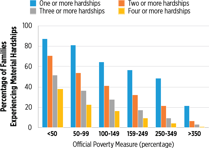
SOURCE: Mayer and Jencks (1989).
TABLE D3-2 Material Hardship
| Author and Year | Source of data | Findings |
|---|---|---|
| Iceland and Bauman, 2007 | Survey of Income and Program Participation, 1996 to 1998 |
|
| Mayer and Jencks, 1989 | Survey Research Laboratory, Northwestern University, 1983 to 1985 |
|
| Gershoff et al., 2007 | Early Childhood Longitudinal Study, 1998 to 1999 |
|
| Ratcliffe and McKernan, 2012 | Panel Study of Income Dynamics, 1968 to 2009 |
|
compared with families who experienced no poverty. Hardships are also likely to coexist for poor families, with 71 percent of families below 50 percent of the federal poverty level (FPL) and 54 percent of families between 50 percent and 99 percent of FPL having two or more material hardships, and 38 percent of those below 50 percent of FPL and 23
percent of those between 50 percent and 99 percent of FPL having four or more hardships (Mayer and Jencks, 1989).
Poverty is significantly correlated with material hardship, which is an important mediator of poverty’s impact on childhood outcomes, at least in early childhood. For example, Gershoff and colleagues (2007) used a nationally representative sample of children developed by the U.S. Department of Education to look at the relationship of income poverty with childhood cognitive skills and social-emotional competence at kindergarten. They also examined the mediating effects of material hardship as well as those of parenting stress, positive parenting, and parental investment in their children. All of these mediators, including material hardship, were partial, meaning that there were still direct effects of poverty on child outcomes. However, material hardship was highly correlated with parenting stress, which negatively impacted parenting behaviors leading to worse outcomes in child social emotional competence. In fact, material hardship explained most of the impact of family income on social-emotional outcomes. Family income had its strongest direct effects on parent investment in their children, which in turn impacted child cognitive skills very strongly (Gershoff et al., 2007).
PHYSICAL HEALTH
Poor children face significant threats to their physical health compared with nonpoor children, starting at birth. They are more likely to be born at a low birth weight and to die during their first year of life; to experience an injury or poisoning requiring medical attention; to have elevated levels of lead in their blood; to experience a chronic disease such as asthma and obesity; and to experience food insecurity (Brooks-Gunn and Duncan, 1997; Chaudry and Wimer, 2016; Moore et al., 2009) (Table D3-3).
Researchers have documented a “gradient” between income and health status, both in children and adults: those with higher income have better health and in the case of adults, longevity (Case, Lubotsky, and Paxson, 2002). In adulthood, the direction of this gradient is difficult to determine. Does poor health lead to low income or does low income lead to poor health? In children, the direction of causality is clearer since children do not contribute to family income in the United States. Researchers have documented an inverse relationship between children’s health and family income, which becomes more negative as the child gets older (Case, Lubotsky, and Paxson, 2002). Even when controlling for parents’ education, the gradients remain strong, so that a doubling of family income increases the likelihood that the child is in very good or excellent health by 4 to 7 percent depending on the age of the child. The U.S. gradient is largest in those children with the most severe chronic conditions (Case, Lubotsky, and Paxson, 2002).
TABLE D3-3 Physical Health
| Author and Year | Source of Data | Findings |
|---|---|---|
| Case, Lubotsky, and Paxson, 2002 | National Health Interview Survey, the 1988 child health supplement to the NHIS, the Panel Study of Income Dynamics with its associated 1997 Child Development Supplement, the Third National Health and Nutrition Examination Survey, 1988 to 1994 |
|
| Currie and Stabile, 2003 | National Longitudinal Survey of Children and Youth, 1994 to 1998 |
|
| Khanam, Nghiem, and Connelly, 2009 | Longitudinal Study of Australian Children, 1999 to 2004 |
|
| Condliffe and Link, 2008 | Medical Expenditure Panel Survey, Panel Study of Income Dynamics, 1996 to 2002 |
|
| Author and Year | Source of Data | Findings |
|---|---|---|
| Ekono, Jiang, and Smith, 2016 | American Community Survey (ACS), the National Health and Nutrition Examination Survey (NHANES), the National Health Interview Survey (NHIS), and the National Survey of Children’s Health (NSCH), 2011 to 2013 |
|
Family income’s relationship to children’s health is in part due to its protection of children’s health on arrival of chronic diseases. In the United States, researchers using the Medical Expenditure Panel Survey (MEPS) as well as the Panel Study of Income Dynamics (PSID) have confirmed that poor children experience more new chronic health conditions than children in wealthier families, but also found that poorer families are less able to respond effectively to these chronic conditions (Case, Lubotsky, and Paxson, 2002). Parental income buffers children from the impacts of chronic diseases, and for almost every chronic condition, children from wealthier families experience better health (Case, Lubotsky, and Paxson, 2002). For example, poor children with asthma in the United States were almost 12 percent more likely to be in poor health 5 years later, whereas children with asthma from a higher-income family were only 4 percent more likely to be in poor health in that same time period (Condliffe and Link, 2008).
Studies from peer English-speaking nations with universal health care have documented a similar relationship between family income and child health, although the magnitude of the relationship is not as pronounced. For example, Currie and Stabile (2003), using a panel of Canadian children, found a flatter gradient between income and child health, although it also steepens as children get older. The data indicate that poor children are subject to more health shocks due to chronic diseases as they get older, which explains the steepening gradient with child age in Canada (Currie and Stabile, 2003). A study of Australian children also confirmed the existence of an income-child health gradient that is flatter than the U.S. gradient (Khanam, Nghiem, and Connelly, 2009). These studies from countries with universal health care indicate that availability of health insurance is not sufficient to eliminate the income gradient in child health, although it appears to reduce it. A more general look at the relationship between income and child health is provided in Institute of Medicine (2013, pp. 2-3).
Children with poorer health also spend less time in school and have fewer years of education, especially if they live in families with lower income (Currie, 2009). Poorer children, due to the income-child health gradient, enter adulthood with poorer health and lower educational attainment, likely leading to lower adult earnings (Case, Lubotsky, and Paxson, 2002). Thus, at least part of the intergenerational transmission of poverty may be due to the impact of family income on children’s health.
FETAL HEALTH AND HEALTH AT BIRTH
There is extensive research indicating that maternal poverty and disadvantage during the prenatal period has an especially significant impact on infant health, one that lasts and affects long-term outcomes (Table D3-4). We know that there are large inequalities in infant health at birth (which can be crudely measured by the incidence of low birth weight) and that these inequalities are associated with socioeconomic factors such as race, maternal education, marital status and income. Defining maternal disadvantage in this way, the incidence of low birth weight is more than three times higher among disadvantaged mothers compared with highly advantaged mothers (Aizer and Currie, 2014).
Maternal health behaviors during pregnancy can impact birth outcomes, and health behaviors during pregnancy are better among mothers with higher incomes. For example, smoking during pregnancy—which has been shown to increase risk of low birth weight and premature birth—is 18 times more prevalent among poor mothers than those who are highly advantaged, and randomized controlled trials of smoking cessation interventions show that reductions in smoking during pregnancy are associated with higher birth weights and less prematurity. Sibling studies (where the mother smoked during one pregnancy and not the other) show similar impact on low birth weight (Aizer and Currie, 2014).
Harmful environmental factors also impact infant health at birth. Studies have consistently shown that poor women are more likely to live near various sources of pollution, such as Superfund hazardous waste sites, factories emitting toxic substances, and water districts with poor drinking-water quality (Currie, 2009). They are also less likely to be able to move to cleaner areas (Currie, 2009; Currie et al., 2013). Natural experiments that change the level of pollution due to policy changes have been shown to reduce the incidence of low birth weight by more than 10 percent (Currie and Walker, 2011).
Maternal health and nutritional status also impact fetal and infant health. Poor women are more likely to have preexisting obesity, diabetes, hypertension, and asthma when they become pregnant (Aizer and Currie, 2014). They are also more likely to be exposed and to be susceptible
TABLE D3-4 Fetal Health and Health at Birth
| Author and Year | Source of data | Findings |
|---|---|---|
| Aizer and Currie, 2014 | U.S. National Individual-Level Natality Data, 2011 |
|
| Currie, 2011 | Environmental Protection Agency’s Toxic Release Inventory, 1989 to 2009 |
|
| Currie et al., 2013 | New Jersey vital statistics natality records, records of drinking water violations for New Jersey, 1997 to 2007 |
|
| Ludwig and Currie, 2010 | Vital Statistics Natality, 1989 to 2003 |
|
(through lack of immunization for example) to contagious diseases like influenza (Currie and Schwandt, 2013). Using data from flu epidemics researchers have shown that influenza during pregnancy has negative effects on infant birth weights, primarily for mothers who have other indicators of poor health. Disadvantaged mothers are also about one-half as likely to gain the recommended weight during pregnancy compared with more advantaged mothers and nutritional interventions during pregnancy have been shown to increase infant birth weight (Ludwig and Currie, 2010).
In summary, there are many reasons that poor women are at increased risk for infants born with lower birth weight, prematurity, and poorer health. Maternal behaviors such as smoking, increased exposure to pollution, and violence, and worse maternal health and nutrition all have negative impacts on infant health at birth. Some studies have also explored the long-term impacts of insults occurring prenatally on infants’ health,
child and adolescent academic achievement, and on adult earnings (Currie and Rossin-Slater, 2015). Finally, we know that nutritional programs such as the Special Supplemental Nutrition Program for Women, Infants, and Children (WIC) and Supplemental Nutritional Assistance Program (SNAP), home visiting programs, and poverty-reduction programs all have proven evidence and/or potential promise to ameliorate these negative outcomes.
BRAIN DEVELOPMENT
Poor children are more likely than other children to have developmental, behavioral, and academic problems, such as serious emotional or behavioral difficulties and learning disabilities (Bradbury et al., 2015; Chaudrey and Wimer, 2016; Heckman, 2006; Moore et al., 2009; Yoshikawa, Aber, and Beardslee, 2012; Table D3-5). It is possible that these outcomes reflect structural brain changes in poor children. Children in poor families have recently been documented to have reduced volumes in the cerebral cortex and hippocampus in areas that are key for school readiness and academic achievement (National Scientific Council on the Developing Child, 2011). These areas are associated with executive function, language development, and memory. Other studies have shown that parental income is related to the surface area of the frontal, temporal, and parietal cortex of children (Noble et al, 2015).
Children growing up in poverty are often exposed to “toxic stress,” which can lead to permanent changes in brain structure and function. Toxic stress is characterized by strong, prolonged activation of the body’s stress response systems (Shonkoff et al., 2012). Poverty causes increased exposure to ACEs and material hardship, as described above, which may induce toxic stress. In addition, parental stress can increase the child’s experience of chronic unbuffered strong stress, which can be especially harmful in the period of rapid brain development that occurs in early childhood (National Council on the Developing Child, 2014; Shonkoff et al., 2012). Toxic stress activates the hormonal systems that respond to stress, especially the hypothalamic-pituitary-adrenocortical (HPA) system, causing sustained high levels of cortisol and corticotropin-releasing hormone, as well as of inflammatory cytokines (Shonkoff et al., 2012). These sustained high levels of stress hormones alter the size and neuronal architecture of the amygdala, hippocampus, and prefrontal cortex, which can lead to functional differences in learning, memory, executive functioning, and to an increased potential for long-term fear and anxiety (Shonkoff et al., 2012).
Elevated exposure to stress appears to modify the physiologic response to stress in ways that alter neuroendocrine activity and neural activity, and ultimately brain development and function, in ways that adversely affect the regulation of emotion and attention (Blair and Raver, 2016). Poor children
TABLE D3-5 Brain Development
| Author and Year | Source of data | Findings |
|---|---|---|
| Noble et al., 2015 | Experimental data |
|
| Mitchell et al., 2014 | Fragile Families and Child Wellbeing Study, 1998 to 2000 |
|
| Theall et al., 2013 | Collected by author, 2010 |
|
experience more chronic stressors and generally manifest higher cortisol and other physiological stress markers than economically advantaged children (Blair et al., 2011; Chen, Cohen, and Miller, 2010; Evans, 2003; Evans and English, 2002; Evans et al., 2005). Exposure to chronic stressors is associated with more externalizing problems and a higher level of behavior problems in children (e.g., Coley, Lynch, and Kull, 2015). Given these connections, it is highly plausible that poverty affects children’s mental health through its effects on brain development (Blair and Raver, 2016).
There is increasing evidence that toxic stress in the prenatal period and early childhood can influence long-term child outcomes by chemically altering the structure and function of genes. These epigenetic changes alter gene expression without altering the genetic code itself, and effectively turn the gene “on” or “off.” These epigenetic changes may be permanent (and some
may be transferred intergenerationally). They may lead to impairments in learning abilities, and increased risk of mental illness, asthma, hypertension, heart disease and diabetes as adults. Not all epigenetic changes are harmful. Research has also shown that positive epigenetic changes in brain cells occur as cognition and memory develop, and repeated stimulation of these brain circuits through positive interactions with the environment and supportive adults (e.g., positive parenting), as well as good prenatal nutrition, enhance these important epigenetic changes (Institute of Medicine, 2000).
One biomarker for chronic stress is telomere length. Telomeres are DNA-protein complexes at the end of chromosomes. Telomeres shorten with age, and toxic stress is believed to accelerate shortening (Mitchell et al., 2014). A study of 9-year-old African American boys compared telomere length in children raised in disadvantaged environments and those in advantaged environments. Growing up in a disadvantaged environment is associated with a 19 percent shorter telomere, whereas a doubling of family income is associated with a 5 percent increase in telomere length (Mitchell et al., 2014).
In addition, severe psychosocial stress in pregnancy has been shown to be associated with shorter telomeres in young adult offspring, and young children exposed to violence have increased telomere shortening when tested at age 10 compared with telomere length when they were 5 (Price et al., 2013). A study of children growing up in poor neighborhoods with a high concentration of poverty, unemployment, and physical disorder documented the association of neighborhood level factors with reduced telomere length as well (Theall et al., 2013). Taken together, these studies provide evidence that chronic stress associated with socioeconomic disadvantage leads to accelerated telomere shortening, especially when experienced early in life. Since telomere length is a proxy for cellular aging, and is associated with diseases like diabetes, cancer, and heart disease, and with psychiatric conditions such as depression, this accelerated telomere shortening associated with poverty puts these children at risk for serious health and mental health problems as they move into adulthood.
MENTAL HEALTH
Numerous correlational studies based on community and national samples and various sources of information about children’s mental health (parent reports, teacher reports, self-reports) show that family-level economic resources are related to children’s mental health, although the associations are generally weaker than for children’s cognitive development and school achievement (e.g., Dubow and Ippolito, 1994; Brooks-Gunn and Duncan, 1997; Pagani, Boulerice, and Tremblay, 1997; Wadsworth et al., 2016; Table D3-6). Children from poor families are at increased risk of
TABLE D3-6 Mental Health
| Author and Year | Source of Data | Findings |
|---|---|---|
| Currie and Tekin, 2015 | Panel Study of Income Dynamics, RealtyTrac, 2005 to 2009 |
|
| Gassman-Pines, Ananat, and Gibson-Davis, 2014 | Youth Risk Behavior Survey, Bureau of Labor Statistics, 1997 to 2009 |
|
| Golberstein, Gonzales, and Meara, 2016 | National Health Interview Survey, 2001 to 2013 |
|
| Gershoff et al., 2007 | Early Childhood Longitudinal Study, 1998 to 1999 |
|
| Mistry et al., 2002 | New Hope Project, 1994 to 1995 |
|
experiencing mental health problems, including depression, difficulties in peer relations, low self-esteem, antisocial behavior, and drug use compared with children in more socioeconomically advantaged families (Bolger et al., 1995; Currie and Lin, 2007; Evans and English, 2002; Gershoff et al., 2007; Goodman, 1999; Goosby, 2007; Strohschein, 2005; Wadsworth et al., 2005; Yoshikawa, Aber, and Beardslee, 2012). Generally, family poverty and other family-level economic indicators are more strongly related to children’s externalizing symptoms (e.g., disobedience, fighting, difficulty
getting along with others, impulsivity) than internalizing symptoms (e.g., anxiety, sadness-depression). Both externalizing symptoms and internalizing symptoms become more prevalent the longer children have been living in poverty (Bolger et al., 1995; Duncan et al., 1994; Goosby, 2007; Hanson, McLanahan, and Thomson, 1997; Korenman, Miller, and Sjaastad, 1995; McLeod and Shanahan, 1993; Pagani, Boulerice, and Tremblay, 1997).
In addition to differences in their income, parents and families who are poor differ in a variety of measured and unmeasured ways. Thus, the links between family income and children’s mental health may reflect these unmeasured differences rather than income differences (Morris and Gennetian, 2003). In virtually all of the studies reviewed here, investigators take some of these differences into account by including control variables (e.g., family structure, maternal education, ethnicity, maternal age at first birth) in their model estimates, which typically reduces the association between income and child mental health. Such studies provide better estimates of the effects of poverty on children than studies without such controls. Nonetheless, these correlational studies are insufficient to establish a causal link between poverty and children’s mental health.
Children’s mental health is related not only to family-level economic indicators, but to area-level economic conditions. These area-level studies focus on economic stressors outside the family, and may help to establish a causal relationship between economic conditions and mental health. However, they generally lack the data necessary to explore processes that account for these associations. In Currie and Tekin’s (2015) study based on administrative hospital data from four states between 2005 and 2009, increases in home foreclosures within zip codes were associated with increases in hospital and emergency room visits for mental health problems among all ages, including children and adolescents. Gassman-Pines and colleagues’ (2014) analysis of data between 1997 and 2009 indicated that statewide job losses due to mass closings and mass layoffs were associated with an increase in the following year in girls’ probability of suicidal ideation and suicide plans, and in non-Hispanic Black adolescents’ probability of suicide attempts. Research also links increases in state-level unemployment rates to greater prevalence of mental health problems among children, controlling for parental mental health (Golberstein, Gonzales, and Meara, 2016).
Correlational studies that link family income and child mental health have produced evidence suggestive of several mediating mechanisms. Most attention has been given to family-based processes that involve material deprivation, parents’ psychological distress, and parenting behavior—processes encapsulated in what is widely known as the “family stress model” (Elder, 1974; Elder and Conger, 1994; for a review of these studies, see Conger, Conger, and Martin, 2010). This model hypothesizes that economic hardship induces strain and pressure in parents. The strain
associated with the daily hassles of making ends meet in turn takes a toll on parents’ mental health, increases interparental conflict and discord, and ultimately interferes with positive parenting, which in turn undermines the child’s mental health.
As examples of empirical support for this model, Gershoff and colleagues’ (2007) investigation based on a representative national sample of kindergarteners showed that higher family income predicted decreased material hardship (e.g., less food insecurity, residential instability, and inadequacy of medical care) and decreased parent stress (i.e., lower levels of marital conflict, parenting stress, depressive symptomatology), which in turn predicted increased positive parenting (i.e., more warmth and cognitive stimulation, less physical punishment) and reduced child problem behaviors. In their ethnically diverse, low-income sample, Mistry and colleagues (2002) found that lower income and increased perceptions of economic pressure affected parenting behavior through an adverse impact on parents’ psychological well-being. Distressed parents reported feeling less effective and capable in disciplinary interactions with their child and were observed to be less affectionate in parent-child interactions. In turn, less than optimal parenting predicted lower teacher ratings of children’s positive social behavior and higher ratings of behavior problems.
Other research into the links between poverty and children’s mental health point to children’s perceptions of family economic difficulties (Dashiff et al., 2009) and their cumulative exposure to stressors (e.g., psychosocial stressors such as family turmoil and community violence, and physical stressors such as substandard housing, high levels of noise, and crowding) (Evans and English, 2002).
Mental health problems in childhood and adolescence, especially externalizing behavior problems, warrant efforts aimed at prevention or early treatment because of their high costs to individuals, families (e.g., costs of treatments), and society (e.g., higher levels of delinquent behavior, crime, and addiction into adulthood) (Golberstein, Gonzales, and Meara, 2016). Their consequences for outcomes in adulthood include lower educational attainment, higher rates of unemployment, and reduced earnings (for a review of these studies, see Currie, 2009). Mental health problems in childhood and adolescence tend to foreshadow mental health problems in adulthood, as data indicate that roughly one-half of all lifetime cases of mental health disorders start in childhood or adolescence (Kessler et al., 2005). Children’s mental health appears to play a significant role in the intergenerational transmission of poverty (Currie, 2009), given evidence linking poverty and low socioeconomic status to parents’ mental health (Lorant et al., 2003, 2007) and children’s mental health and the association between child mental health, future education, and labor market outcomes (Currie, 2009).
EDUCATIONAL ATTAINMENT
Innumerable studies have documented a gap in the average achievement levels of students from low-income families relative to high-income families (Table D3-7). This gap appears in virtually all measures of achievement including grades, standardized test scores, high school graduate rates, college attendance, and college graduation rates (Bradbury et al., 2015; Chaudry and Wimer, 2016; Haveman and Wolfe, 1995; Heckman, 2006; Moore et al., 2009; Yoshikawa, Aber, and Beardslee, 2012).
Alarmingly, Reardon (2013) documents the fact that this income-achievement gap is not stable, but has been increasing steadily over the past 50 years. He shows that the gap in achievement between a child at the 90th percentile of the family income distribution and a child at the 10th percentile of the family income distribution is almost twice as big as the gap in achievement between white and African-American students—while 50 years ago the situation was reversed.
This gap in achievement is present when children enter kindergarten and stays relatively stable over time, indicating that the gap has its origins in the preschool period. Indeed Hair et al. (2015) suggest that differences in brain volume in the frontal and temporal cortex can explain 15–20 percent of the difference in scores between poor and nonpoor children, suggesting that intervention during periods of peak brain development in early childhood may be key.
RISKY BEHAVIORS, CRIME, AND DELINQUENCY
Poverty is linked to adolescent delinquency independent of other familial factors such as maternal education, family configuration status, and earlier childhood behavior patterns (Pagani et al., 1999; Table D3-8). In general, this link is stronger when the dependent variable is serious delinquency (Bjerk, 2007; Farnworth et al., 1994; Jarjoura, Triplett, and Brinker, 2002), if youth live in persistent poverty (Duncan et al., 1994; Farnworth et al., 1994; Jarjoura, Triplett, and Brinker, 2002), and if adolescents experienced poverty during early childhood or during adolescence (Brooks-Gunn and Duncan, 1997; Duncan et al, 1998; Jarjoura, Triplett, and Brinker, 2002).
Bjerk’s (2007) systematic analyses suggest that the association between income and delinquency can be obscured because of its nonlinearity and because of error in the measurement of household economic resources. Dividing household income into quintiles, he found a negative relationship between household income and participation in serious crime (e.g., assault, stealing with a weapon or use of force, selling “hard drugs”) only when comparing adolescents at the lowest end of the income distribution
TABLE D3-7 Educational Attainment
| Author and Year | Source of Data | Findings |
|---|---|---|
| Reardon, 2013 | National Center for Education Statistics (NCES), the Long-Term Trend and Main National Assessment of Educational Progress (NAEP) studies, 1943 to 2001 |
|
| Hair et al., 2015 | National Institutes of Health Magnetic Resonance Imaging Study of Normal Brain Development, 2001 to 2007 |
|
| Votruba-Drzal, 2006 | National Longitudinal Survey of Youth, 1986 to 2000 |
|
| Brooks-Gunn and Duncan, 1997 | National Longitudinal Survey of Youth, Infant Health and Development Program, 1997 |
|
| Ratcliffe and McKernan, 2012 | Panel Study of Income Dynamics, 1968 to 2009 |
|
TABLE D3-8 Risky Behaviors, Crime, and Delinquency
| Author and Year | Source of Data | Findings |
|---|---|---|
| Pagani et al., 1999 | Montreal Longitudinal-Experimental Study, 1984 to 1993 |
|
| Bjerk, 2007 | National Longitudinal Survey of Children and Youth, 1997 |
|
| Jarjoura, Triplett, and Brinker, 2002 | National Longitudinal Survey of Children and Youth, 1979 to 1992 |
|
| Blum et al., 2000 | National Longitudinal Survey of Children and Youth |
|
| Author and Year | Source of Data | Findings |
|---|---|---|
| Bartlett, Holditch-Davis, and Belyea, 2005 | National Longitudinal Study of Adolescent Health |
|
| Ratcliffe and McKernan, 2012 | Panel Study of Income Dynamics, 1968 to 2009 |
|
with those at the highest end of the income distribution. In addition, the relationship was much stronger if the measure of family economic well-being included other family economic indicators in addition to income (e.g., savings, debts owed, inheritances). Household income and participation in minor crime (e.g., stealing without force or threat of force, property destruction) were unrelated.
Family poverty in middle childhood appears to be less important as an antecedent to serious delinquency than poverty during early childhood or adolescence (Jarjoura, Triplett, and Brinker, 2002). Several studies show that much of the increased risk of delinquency associated with poverty is mediated through negative parenting and family conflict (e.g., harshness, inconsistency, low monitoring and involvement) (Conger et al., 1994, 1995;
Rutter, Giller, and Hagell, 1998; Sampson and Laub, 1994), though this mediation is not found in some studies (e.g., Pagani et al., 1999).
Several studies have found that official intervention (e.g., being arrested or convicted) during adolescence is negatively associated with employment in early adulthood (Aizer and Doyle, 2015). Moreover, analyses of panel data suggest that official intervention increases involvement in crime in early adulthood by adversely affecting educational attainment and employment. Declines in educational progress following official intervention may be triggered by stigma and exclusion from school. Increases in crime in response to official intervention appear to be especially pronounced among African American males and males who come from poor family backgrounds (Bernburg and Krohn, 2003).
Delinquency is one of a group of adolescent risky behaviors that are correlated and tend to co-occur (Gruber, 2001; Jessor, Turbin, and Costa, 1998). This co-occurrence has stimulated research on domains and profiles of adolescent risky behavior and their antecedents and outcomes in early adulthood (e.g., Bartlett, Holditch-Davis, and Belyea, 2005; Hair et al., 2009; Zweig, Lindberg, and McGinley, 2001). Blum et al. (2000) focused specifically on health-compromising behaviors among 7th–12th graders (e.g., alcohol use, cigarette smoking, suicidal thoughts or attempts, weapon-related violence, sexual intercourse) in the National Longitudinal Study of Adolescent Health (Add Health). Lower family income was associated with less alcohol use (among 9th–12th graders), but higher weapon-related violence, and greater likelihood of sexual intercourse, controlling for demographic variables related to family income. However, family income, family structure, and race/ethnicity, taken together, explained very little of the variance in these outcomes.
Using data from over 12,500 adolescents from Add Health, Bartlett, Holditch-Davis, and Belyea (2005) identified three clusters of youth (mean age 15.8 years) based on 14 problem behaviors, including delinquency (e.g., stealing, weapon use, property damage), alcohol and marijuana use, sexual behavior (e.g., multiple sex partners, sex without birth control) and truancy. Youth in the “normal” cluster reported few, if any problem behaviors; those in the “deviant” cluster had high means for most of the behaviors and the largest number of problem behaviors reflecting deviant, conduct-type problems like selling drugs and weapon use; youth in the “problem” cluster had higher means than those in the “normal” cluster for most problems, but lower means than youth in the “deviant” cluster. Family SES was a significant predictor of cluster membership, with adolescents in the “normal” cluster having significantly higher SES than adolescents in the “deviant” and “problem” clusters. Other research distinguishing profiles of risky behavior among adolescents (based on delinquency, smoking, drug use, drinking, sexual behavior, etc.) finds worse adult outcomes (e.g., increased
probability of arrest, not having a high school diploma or GED, not being employed) among those in higher-risk groups, compared with those in lower-risk groups (Hair et al., 2009).
Early timing of events beyond sexual debut has been conceptualized as a marker of risky behavior (e.g., parenthood) because these early transitions often create demands and conditions that place individuals at increased risk for low education and enduring occupational, financial, and attendant stressors that compromise psychological health (McLoyd, Purtell, and Hardaway, 2015). Research confirms that family poverty and low socioeconomic status increase the probability of early timing of transition events (e.g., sexual intercourse by age 14; pregnancy, parenthood, cohabitation, marriage, or leaving the parental home by age 17) partly by increasing the occurrence of negative life events experienced by parents or the family (e.g., getting laid off, taking wage cuts, moving to worse residences or neighborhoods). In turn, early timing of transition events has been found to predict significant growth in depressive symptoms in early adulthood (Wickrama, Merten, and Elder, 2005; Wickrama et al., 2008).
THE TIMING OF POVERTY
The timing of poverty is important. Early childhood is a period when brain development is rapid, and children are very sensitive to the impacts of family poverty (Blair and Raver, 2016). Language development diverges for poor and nonpoor children almost as soon as expressive language emerges at 15 or 16 months of age, and by 3 years of age poor children are markedly behind in their language acquisition (Hart and Risley, 1995). One recent study indicated that differences in language development between poor and nonpoor children can be seen as early as 7 months of age (Betancourt, Brodsky, and Hurt, 2015). Another study looking at EEG37 patterns found decreased electrical activity in the frontal cortex, the part of the brain that controls executive function, in poor 6- to 9-month-olds compared with those living in families with higher income (Tomalski et al., 2013). The impacts of poverty experienced early in childhood last into adulthood. Poverty in early childhood has been shown to be a very significant negative predictor of academic performance in school in middle childhood and beyond. The reading and math skills of children experiencing poverty in early life diverge over time from the skills of more advantaged children during the school years (Votruba-Drzal, 2006). Children who are poor from birth to age 2 are 30 percent less likely to graduate from high school and are three times more likely to have a teen premarital pregnancy (Ratcliffe and
___________________
37 An EEG, or electroencephalogram, is a neurological test that detects abnormalities in the brain’s electrical activity.
McKernan, 2012). These outcomes are likely to lead to less employment as adults and to intergenerational poverty. And poverty in early childhood is likely to persist. Nearly one-half of children born to poor parents remain poor for one-half or more of their childhoods (Ratcliffe and McKernan, 2012).
Nevertheless, poverty experienced later in childhood is also associated with negative outcomes in adolescence and adulthood, perhaps in part because the length of time a child spends in poverty is also important. Experiencing persistent poverty (for one-half or more of childhood years) is associated with not graduating from high school, having teen nonmarital births and nonmarital births as adults for females, and with higher arrest rates by young adulthood for males (Ratcliffe and McKernan, 2012). As with poverty experienced in early childhood, these outcomes lead to lower earnings as adults and an increased likelihood of long-term adult poverty and poorer adult health (Chaudry and Wimer, 2016; Ratcliffe and McKernan, 2012). The longer the duration of poverty, the more likely the child will have these negative outcomes.
SEVERITY OF POVERTY
In 2015, 2.9 percent of children in the United States, or 2.1 million children,38 lived in deep poverty, that is, had family income less than 50 percent of the Supplemental Poverty Measure. Families living in deep poverty experience even greater material hardship and parenting stress than those who are poor but living between 50 percent and 99 percent of the federal poverty level (Mayer and Jencks, 1989). Young children growing up in deep poverty have higher rates of obesity, and three times the rate of elevated blood lead levels compared with other poor children (Ekono, Jiang, and Smith, 2016). One study showed that children in deep poverty had scores 6 to 13 points lower on standardized tests of IQ, verbal ability, and achievement compared with nonpoor children. Scores for children living in poverty but above deep poverty were also lower than those who were nonpoor, but the differences were not as large (Brooks-Gunn and Duncan, 1997).
Children in deep poverty also are more likely to grow up in families with significant additional risk factors. Compared with poor children not in deep poverty, they are more likely to have parents reporting poor or fair health and mental health, more parental stress, less social support, and living in unsafe neighborhoods (Ekono, Jiang, and Smith, 2016). These factors predict poor health and development outcomes in children. The combination of deep poverty and family adversity is particularly toxic (Ekono, Jiang, and Smith, 2016).
___________________
38 Per TRIM3 weighted estimates commissioned for the committee.
REFERENCES
Aizer, A. (2011). Poverty, violence and health: The impact of domestic violence during pregnancy on newborn health. Journal of Human Resources, 46(3), 518–538.
Aizer, A., and Currie, J. (2014). The intergenerational transmission of inequality: Maternal disadvantage and health at birth. Science, 344(6186), 856–861.
Aizer, A., and Doyle, J.J. (2015). Juvenile incarceration, human capital, and future crime: Evidence from randomly assigned judges. Quarterly Journal of Economics, 130(2), 759–803.
Almond, D., and Currie, J. (2011). Killing me softly: The fetal origins hypothesis. Journal of Economic Perspectives, 25(3), 153–172.
Anda, R.F., Felitti, V.J., Bremner, J.D., Walker, J.D., Whitfield, C., Perry, B.D., Dube, S.R., and Giles, W.H. (2006). The enduring effects of abuse and related adverse experiences in childhood: A convergence of evidence from neurobiology and epidemiology. European Archives of Psychiatry and Clinical Neuroscience, 256(3), 174–186.
Bartlett, R., Holditch-Davis, D., and Belyea, M. (2005). Clusters of problem behaviors in adolescents. Research in Nursing and Health, 28(3), 230–239.
Bernburg, J.G., and Krohn, M.D. (2003). Labeling, life chances, and adult crime: The direct and indirect effects of official intervention in adolescence on crime in early adulthood. Criminology, 41(4), 1287–1318.
Betancourt, L.M., Brodsky, N.L., and Hurt, H. (2015). Socioeconomic (SES) differences in language are evident in female infants at 7 months of age. Early Human Development, 91(12), 719–724.
Bjerk, D. (2007). Measuring the relationship between youth criminal participation and household economic resources. Journal of Quantitative Criminology, 23(1), 23–39.
Blair, C., and Raver, C.C. (2016). Poverty, stress, and brain development: New directions for prevention and intervention. Academic Pediatrics, 16(3 Suppl), S30–36.
Blair, C., Raver, C.C., Granger, D., Mills-Koonce, R., and Hibel, L. (2011). Allostasis and allostatic load in the context of poverty in early childhood. Developmental Psychopathology, 23(3), 845–857.
Blum, R.W., Beuhring, T., Shew, M.L., Bearinger, L.H., Sieving, R.E., and Resnick, M.D. (2000). The effects of race/ethnicity, income, and family structure on adolescent risk behaviors. American Journal of Public Health, 90(12), 1879–1884.
Bolger, K.E., Patterson, C.J., Thompson, W.W., and Kupersmidt, J.B. (1995). Psychosocial adjustment among children experiencing persistent and intermittent family economic hardship. Child Development, 66(4), 1107–1129.
Bradbury, B., Corak, M., Waldfogel, J., and Washbrook, E. (2015). Too Many Children Left Behind: The U.S. Achievement Gap in Comparative Perspective. New York, NY: Russell Sage Foundation.
Brooks-Gunn, J., and Duncan, G.J. (1997). The effects of poverty on children. Future Child, 7(2), 55–71.
Cancian, M., Yang, M.Y., and Slack, K.S. (2013). The effect of additional child support income on the risk of child maltreatment. Social Service Review, 87(3), 417–437.
Case, A., Lubotsky, D., and Paxson, C. (2002). Economic status and health in childhood: The origins of the gradient. American Economic Review, 92(5), 1308–1334.
Chaudry, A., and Wimer, C. (2016). Poverty is not just an indicator: The relationship between income, poverty, and child well-being. Academic Pediatrics, 16(3 Suppl), S23–29.
Chen, E., Cohen, S., and Miller, G.E. (2010). How low socioeconomic status affects 2-year hormonal trajectories in children. Psychological Science, 21(1), 31–37.
Coley, R.L., Lynch, A.D., and Kull, M. (2015). Early exposure to environmental chaos and children’s physical and mental health. Early Childhood Research Quarterly, 32, 94–104.
Condliffe, S., and Link, C.R. (2008). The relationship between economic status and child health: Evidence from the United States. American Economic Review, 98(4), 1605–1618.
Conger, R.D., Conger, K.J., and Martin, M.J. (2010). Socioeconomic status, family processes, and individual development. Journal of Marriage and Family, 72(3), 685–704.
Conger, R.D., Ge, X., Elder, G.H., Jr., Lorenz, F.O., and Simons, R.L. (1994). Economic stress, coercive family process, and developmental problems of adolescents. Child Development, 65(2 Spec No), 541–561.
Conger, R.D., Patterson, G.R., and Ge, X. (1995). It takes two to replicate: A mediational model for the impact of parents’ stress on adolescent adjustment. Child Development, 66(1), 80–97.
Currie, J. (2011). Inequality at birth: Some causes and consequences. American Economic Review, 101(3), 1–22.
Currie, J. (2009). Healthy, wealthy, and wise: Socioeconomic status, poor health in childhood, and human capital development. Journal of Economic Literature, 47(1), 87–122.
Currie, J., and Lin, W. (2007). Chipping away at health: More on the relationship between income and child health. Health Affairs (Millwood), 26(2), 331–344.
Currie, J., and Rossin-Slater, M. (2015). Early-life origins of life-cycle well-being: Research and policy implications. Journal of Policy Analysis and Management, 34(1), 208–242.
Currie, J., and Schwandt, H. (2013). Within-mother analysis of seasonal patterns in health at birth. Proceedings of the National Academy of Sciences, 110(30), 12265–12270.
Currie, J., and Stabile, M. (2003). Socioeconomic status and child health: Why is the relationship stronger for older children? American Economic Review, 93(5), 1813–1823.
Currie, J., and Tekin, E. (2015). Is there a link between foreclosure and health? American Economic Journal: Economic Policy, 7(1), 63–94.
Currie, J., and Walker, R. (2011). Traffic congestion and infant health: Evidence from E-ZPass. American Economic Journal-Applied Economics, 3(1), 65–90.
Currie, J., Zivin, J.G., Meckel, K., Neidell, M., and Schlenker, W. (2013). Something in the water: Contaminated drinking water and infant health. Canadian Journal of Economics, 46(3). https://doi.org/10.1111/caje.12039.
Dashiff, C., DiMicco, W., Myers, B., and Sheppard, K. (2009). Poverty and adolescent mental health. Journal of Child and Adolescent Psychiatric Nursing, 22(1), 23–32.
Dubow, E.F., and Ippolito, M.F. (1994). Effects of poverty and quality of the home-environment on changes in the academic and behavioral-adjustment of elementary school-age-children. Journal of Clinical Child Psychology, 23(4), 401–412.
Duncan, G., Brooks-Gunn, J., and Klebanov, P. (1994). Economic deprivation and early childhood development. Child Development, 65, 296–318.
Duncan, G.J., Yeung, W.J., Brooks-Gunn, J., and Smith, J.R. (1998). How much does childhood poverty affect the life chances of children? American Sociological Review, 63(3), 406.
Ekono, M.M., Jiang, Y., and Smith, S. (2016). Young Children in Deep Poverty. New York: National Center for Children in Poverty, Columbia University. Available: https://files.eric.ed.gov/fulltext/ED578993.pdf.
Elder, G.H. (1974). Children of the Great Depression. Chicago: University of Chicago Press.
Elder Jr., G.H., and Conger, R.D. (1994). Families in Troubled Times: Adapting to Change in Rural America. Social Institutions and Social Change. Piscataway, NJ: Aldine Transaction.
Evans, G.W. (2003). A multimethodological analysis of cumulative risk and allostatic load among rural children. Developmental Psychology, 39(5), 924–933.
Evans, G.W., and English, K. (2002). The environment of poverty: Multiple stressor exposure, psychophysiological stress, and socioemotional adjustment. Child Development, 73(4), 1238–1248.
Evans, G.W., Gonnella, C., Marcynyszyn, L.A., Gentile, L., and Salpekar, N. (2005). The role of chaos in poverty and children’s socioemotional adjustment. Psychological Science, 16(7), 560–565.
Farnworth, M., Thornberry, T., Krohn, M., and Lizotte, A. (1994). Measurement in the study of class and delinquency: Integrating theory and research. Journal of Research in Crime and Delinquency, 31(1), 32–61.
Gassman-Pines, A., Ananat, E.O., and Gibson-Davis, C.M. (2014). Effects of statewide job losses on adolescent suicide-related behaviors. American Journal of Public Health, 104(10), 1964–1970.
Gershoff, E.T., Aber, J.L., Raver, C.C., and Lennon, M.C. (2007). Income is not enough: Incorporating material hardship into models of income associations with parenting and child development. Child Development, 78(1), 70–95.
Golberstein, E., Gonzales, G., and Meara, E. (2016). Economic Conditions and Children’s Mental Health. Cambridge, MA: National Bureau of Economic Research.
Goodman, E. (1999). The role of socioeconomic status gradients in explaining differences in US adolescents’ health. American Journal of Public Health, 89(10), 1522–1528.
Goosby, B.J. (2007). Poverty duration, maternal psychological resources, and adolescent socioemotional outcomes. Journal of Family Issues, 28(8), 1113–1134.
Gruber, J. (2001). Risky Behavior Among Youths. Chicago: University of Chicago Press.
Hair, E.C., Park, M.J., Ling, T.J., and Moore, K.A. (2009). Risky behaviors in late adolescence: Co-occurrence, predictors, and consequences. Journal of Adolescent Health, 45(3), 253–261.
Hair, N.L., Hanson, J.L., Wolfe, B.L., and Pollak, S.D. (2015). Association of child poverty, brain development, and academic achievement. JAMA Pediatrics, 169(9), 822–829.
Hanson, T., McLanahan, S., and Thomson, E. (1997). Economic resources, parental practices, and children’s well-being. In G. Duncan and J. Brooks-Gunn (Eds.), Consequences of Growing Up Poor. New York: Russell Sage Foundation.
Hart, B., and Risley, T.R. (1995). Meaningful Differences in the Everyday Experience of Young American Children. Baltimore, MD: Paul H Brookes Publishing.
Haveman, R., and Wolfe, B. (1995). The determinants of children’s attainments: A review of methods and findings. Journal of Economic Literature, 33(4), 1829–1878.
Heckman, J.J. (2006). Skill formation and the economics of investing in disadvantaged children. Science, 312(5782), 1900–1902.
Iceland, J., and Bauman, K.J. (2007). Income poverty and material hardship: How strong is the association? The Journal of Socio-Economics, 36(3), 376–396.
Institute of Medicine. (2013). U.S. Health in International Perspective—Shorter Lives, Poorer Health Report Brief, January. Washington, DC: The National Academies Press. Available: http://www.nationalacademies.org/hmd/~/media/Files/Report%20Files/2013/US-Health-International-Perspective/USHealth_Intl_PerspectiveRB.pdf.
Institute of Medicine (2000). From Neurons to Neighborhoods: The Science of Early Childhood Development. Washington, DC: National Academy Press.
Jarjoura, G.R., Triplett, R.A., and Brinker, G.P. (2002). Growing up poor: Examining the link between persistent childhood poverty and delinquency. Journal of Quantitative Criminology, 18(2), 159–187.
Jessor, R., Turbin, M.S., and Costa, F.M. (1998). Risk and protection in successful outcomes among disadvantaged adolescents. Applied Developmental Science, 2(4), 194–208.
Kessler, R.C., Berglund, P., Demler, O., Jin, R., Merikangas, K.R., and Walters, E.E. (2005). Lifetime prevalence and age-of-onset distributions of DSM-IV disorders in the national comorbidity survey replication. Archives of General Psychiatry, 62(6), 593–602.
Khanam, R., Nghiem, H.S., and Connelly, L.B. (2009). Child health and the income gradient: Evidence from Australia. Journal of Health Economics, 28(4), 805–817.
Korenman, S., Miller, J.E., and Sjaastad, J.E. (1995). Long-term poverty and child development in the United States: Results from the NLSY. Children and Youth Services Review, 17(1), 127–155.
Lorant, V., Deliege, D., Eaton, W., Robert, A., Philippot, P., and Ansseau, M. (2003). Socioeconomic inequalities in depression: A meta-analysis. American Journal of Epidemiology, 157(2), 98–112.
Lorant, V., Croux, C., Weich, S., Deliege, D., Mackenbach, J., and Ansseau, M. (2007). Depression and socio-economic risk factors: 7-year longitudinal population study. British Journal of Psychiatry, 190, 293–298.
Ludwig, D.S., and Currie, J. (2010). The association between pregnancy weight gain and birthweight: A within-family comparison. Lancet, 376(9745), 984–990.
Macomber, J. (2006). An Overview of Selected Data on Children in Vulnerable Families. Washington, DC: Urban Institute.
Mayer, S.E., and Jencks, C. (1989). Poverty and the distribution of material hardship. Journal of Human Resources, 24(1), 88–114.
McLeod, J.D., and Shanahan, M.J. (1993). Poverty, parenting, and children’s mental health. American Sociological Review, 351–366.
McLoyd, V.C., Purtell, K.M., and Hardaway, C.R. (2015). Race, class, and ethnicity in young adulthood. In Handbook of Child Psychology and Developmental Science. Hoboken, NJ: John Wiley and Sons.
Mistry, R.S., Vandewater, E.A., Huston, A.C., and McLoyd, V.C. (2002). Economic well-being and children’s social adjustment: The role of family process in an ethnically diverse low-income sample. Child Development, 73(3), 935–951.
Mitchell, C., Hobcraft, J., McLanahan, S.S., Siegel, S.R., Berg, A., Brooks-Gunn, J., Garfinkel, I., and Notterman, D. (2014). Social disadvantage, genetic sensitivity, and children’s telomere length. Proceedings of the National Academy of Sciences, 111(16), 5944–5949.
Moore, K.A., Redd, Z., Burkhauser, M., Mbwana, K., and Collins, A. (2009). Children in Poverty: Trends, Consequences, and Policy Options. Washington, DC: Child Trends.
Morris, P.A., and Gennetian, L.A. (2003). Identifying the effects of income on children’s development using experimental data. Journal of Marriage and Family, 65(3), 716–729.
National Scientific Council on the Developing Child (2011). Building the Brain’s “Air Traffic Control” System: How Early Experiences Shape the Development of Executive Function. Cambridge, MA: Harvard University.
National Scientific Council on the Developing Child (2014). Excessive Stress Disrupts the Architecture of the Developing Brain: Working Paper 3 Updated Edition. Cambridge, MA: Harvard University. Available: https://developingchild.harvard.edu/wp-content/uploads/2005/05/Stress_Disrupts_Architecture_Developing_Brain-1.pdf [August 30, 2018].
National Survey of Children’s Health 2011/12. (2017). Adverse Childhood Experiences. Data query from the Child and Adolescent Health Measurement Initiative, Data Resource Center for Child and Adolescent Health website. Retrieved September 28, 2018 from www.childhealthdata.org.
Noble, K.G., Houston, S.M., Brito, N.H., Bartsch, H., Kan, E., Kuperman, J.M., Akshoomoff, N., Amaral, D.G., Bloss, C.S., Libiger, O., Schork, N.J., Murray, S.S., Casey, B.J., Chang, L., Ernst, T.M., Frazier, J.A., Gruen, J.R., Kennedy, D.N., Van Zijl, P., Mostofsky, S., Kaufmann, W.E., Kenet, T., Dale, A.M., Jernigan, T.L., and Sowell, E.R. (2015). Family income, parental education and brain structure in children and adolescents. Nature Neuroscience, 18(5), 773–778.
Ouellette, T., Burstein, N., Long, D., and Beecroft, E. (2004). Measures of Material Hardship: Final Report. Washington, DC: US Department of Health and Human Services, Office of the Assistant Secretary for Planning and Evaluation.
Pagani, L., Boulerice, B., Tremblay, R. (1997). The influence of poverty on children’s classroom placement and behavior problems. In G.J. Duncan and J. Brooks-Gunn (Eds.), Consequences of Growing Up Poor (pp. 311–329). New York: Russell Sage Foundation.
Pagani, L., Boulerice, B., Vitaro, F., and Tremblay, R.E. (1999). Effects of poverty on academic failure and delinquency in boys: A change and process model approach. Journal of Child Psychology and Psychiatry, 40(8), 1209–1219.
Paxson, C., and Waldfogel, J. (2003). Welfare reforms, family resources, and child maltreatment. Journal of Policy Analysis and Management, 22(1), 85–113.
Price, L.H., Kao, H.T., Burgers, D.E., Carpenter, L.L., and Tyrka, A.R. (2013). Telomeres and early-life stress: An overview. Biological Psychiatry, 73(1), 15–23.
Ratcliffe, C.E., and McKernan, S.M. (2012). Child Poverty and Its Lasting Consequence. Washington, DC: Urban Institute. Available: https://www.urban.org/sites/default/files/publication/32756/412659-Child-Poverty-and-Its-Lasting-Consequence.PDF.
Reardon, S.F. (2013). The widening income achievement gap. Educational Leadership, 70(8), 10–16.
Rutter, M., Giller, H., and Hagell, A. (1998). Antisocial Behaviour by Young People. New York, NY: Cambridge University Press.
Sampson, R.J., and Laub, J.H. (1994). Urban poverty and the family context of delinquency: A new look at structure and process in a classic study. Child Development, 65(2 Spec No), 523–540.
Sedlak, A.J., Mettenburg, J., Basena, M., Petta, I., McPherson, K., Greene, A., and Li, S. (2010). Fourth National Incidence Study of Child Abuse and Neglect (NIS-4): Report to Congress: Executive Summary. Washington, DC: U.S. Department of Health and Human Services. Available: https://www.acf.hhs.gov/sites/default/files/opre/nis4_report_congress_full_pdf_jan2010.pdf [August 30, 2018].
Shonkoff, J.P., Garner, A.S., Committee on Psychosocial Aspects of Child and Family Health, Committee on Early Childhood, Adoption and Family Care, and Section on Developmental and Behavioral Pediatrics. (2012). The lifelong effects of early childhood adversity and toxic stress. Pediatrics, 129(1), e232–e246.
Strohschein, L. (2005). Household income histories and child mental health trajectories. Journal of Health and Social Behavior, 46(4), 359–375.
Theall, K.P., Brett, Z.H., Shirtcliff, E.A., Dunn, E.C., and Drury, S.S. (2013). Neighborhood disorder and telomeres: Connecting children’s exposure to community level stress and cellular response. Social Science and Medicine, 85, 50–58.
Tomalski, P., Moore, D.G., Ribeiro, H., Axelsson, E.L., Murphy, E., Karmiloff-Smith, A., Johnson, M.H., and Kushnerenko, E. (2013). Socioeconomic status and functional brain development—associations in early infancy. Developmental Science, 16(5), 676–687.
Votruba-Drzal, E. (2006). Economic disparities in middle childhood development: Does income matter? Developmental Psychology, 42(6), 1154–1167.
Wadsworth, M.E., Evans, G.W., Grant, K., Carter, J.S., and Duffy, S. (2016). Poverty and the development of psychopathology. In D. Cicchetti (Ed.), Developmental Psychopathology (pp. 136–179, 3rd edition). Hoboken, NJ: Wiley.
Wadsworth, M.E., Raviv, T., Compas, B.E., and Connor-Smith, J.K. (2005). Parent and adolescent responses to poverty related stress: Tests of mediated and moderated coping models. Journal of Child and Family Studies, 14(2), 283–298.
Wickrama, K.A.S., Merten, M.J., and Elder, G.H. Jr. (2005). Community influence on precocious transitions to adulthood: Racial differences and mental health consequences. Journal of Community Psychology, 33(6), 639–653.
Wickrama, K.A.S., Conger, R.D., Lorenz, F.O., and Jung, T. (2008). Family antecedents and consequences of trajectories of depressive symptoms from adolescence to young adulthood: A life course investigation. Journal of Health and Social Behavior, 49(4), 468–483.
Yoshikawa, H., Aber, J.L., and Beardslee, W.R. (2012). The effects of poverty on the mental, emotional, and behavioral health of children and youth: Implications for prevention. American Psychologist, 67(4), 272–284.
Zweig, J.M., Lindberg, L.D., and McGinley, K.A. (2001). Adolescent health risk profiles: The co-occurrence of health risks among females and males. Journal of Youth and Adolescence, 30(6), 707–728.
APPENDIX D, 4-1
DEFINITIONS PERTAINING TO CHAPTER 4 FROM THE ORGANISATION FOR ECONOMIC CO-OPERATION AND DEVELOPMENT (OECD)
Definition of OECD Family Benefits Public Spending39
Figure 4-12 in Chapter 4 of this report presents data on public spending on families and children as a percent of the Gross Domestic Product (GDP). This is based on an indicator known as OECD Family Benefits Public Spending, which refers to public spending on family benefits, including financial support that is exclusively for families and children. Spending on health and housing also assists families, but not exclusively, and it is not included in this indicator. Broadly speaking, there are three types of public spending on family benefits:
- Public spending on child-related cash transfers to families with children, including child benefits (or child allowances) that in some countries are income-tested; public income support payments for single-parent families; and income support issued during periods of parental leave.
- Public spending on services (benefits in kind) for families with children, including direct financing and subsidizing of providers of child care and early education facilities; public child care support through earmarked payments to parents; public spending on assistance for young people and residential facilities; public spending on family services, including center-based facilities; and home help services for families in need.
- Financial support for families provided through the tax system, including tax exemptions (e.g., income from child benefits that is not included in the tax base); child tax allowances (amounts for children that are deducted from gross income and are not included in taxable income); and child tax credits, amounts that are deducted from the tax liability.
This indicator can be broken down by cash benefits and benefits in kind and is measured in percentage of GDP.
___________________
39 See https://data.oecd.org/socialexp/family-benefits-public-spending.htm.
APPENDIX D, 4-2
GOVERNMENT POLICIES AFFECTING CHILD POVERTY IN AUSTRALIA AND IRELAND
The Australian Family Tax Benefit, Parts A and B
The Australian government provides a family tax benefit to families with children based on specific eligibility criteria. This family benefit is intended to assist with the cost of raising children and consists of two parts, A and B. Overall eligibility criteria include these: (1) the parent(s) have a dependent child or full-time student under the age of 20 who does not receive a pension, payment, or other benefits; (2) the parent(s) are providing care for the child at least 35 percent of the time; and (3) the family meets a specific income test.40 The income test for this program, and for Australian transfer programs in general, is designed to eliminate eligibility only for very-high-income families. Consequently, it is a near universal benefit and is classified by OECD as such. Part A is given for each child in families that meet the eligibility criteria, and Part B is intended to provide additional assistance to single parents, nonparental caregivers, and couples with one earner. In order to receive Part A, children must also meet immunization requirements.
According to a United Nations Children’s Fund (UNICEF) report on the impact of the worldwide financial/economic crisis on child well-being in 41 high-income countries (Fanjul, 2014), based on an anchored poverty line Australia experienced the third-best improvement over the 2008–2012 period, with its child poverty rate falling from just over 19 percent to 13 percent. During this 4-year period, Australia moved from having the 19th-lowest rate to the 7th-lowest rate of child poverty. The UNICEF report highlights that Australia had a multipronged approach, which included countercyclical policies to alleviate the effects of the economic downturn as well as stimulus packages that were targeted to low-income families with children.
However, there is concern that going forward, Australia’s outcomes may not be as positive. In 2009, the indexation of Family Tax Benefit Part A was made less generous, leading to a decline in the number of children benefiting from it, which fell from about 80 percent of all dependent children in 2009 to about 69 percent in 2012 (Whiteford, 2014).
___________________
40 Australian Government Department of Human Services, https://www.humanservices.gov.au/individuals/services/centrelink/family-tax-benefit.
Ireland’s National Policy Framework for Children and Young People
In 2014, Ireland’s government established the goal of lifting 70,000 children out of poverty by the year 2020, part of its National Policy Framework for Children and Young People, also known as the Better Outcomes, Brighter Futures (BOBF) Framework (Ireland, Department of Employment Affairs and Social Protection, 2017). This is based on 2013 guidance from the European Commission that set out a three-pronged framework to address child poverty. These prongs were “access to adequate resources; access to affordable quality services; and children’s right to participate.” (Ireland, Department of Employment Affairs and Social Protection, 2017, p. 11).
With regard to adequate resources, Ireland provides a number of different income supports for families with children. The government offers a Child Benefit, which is a monthly payment payable to the parents or guardians of children under the age of 16, or under the age of 18 if the child is in full-time education, full-time training, or with a disability and cannot support themselves (Ireland, Department of Employment Affairs and Social Protection, 2018). Ireland also offers:
- Increases in some social welfare payments for each qualified child,
- Family Income Supplement,
- Back to School Clothing and Footwear Allowance,
- School Meals,
- Back to Work Family Dividend (allowing parents to combine welfare and work),
- Domiciliary Care Allowance (for children under age 16 with a severe disability),
- Fuel Allowance, and
- Exceptional Needs Payments (Ireland, Department of Employment Affairs and Social Protection, 2017).
The Irish government also has programs intended to make quality child care more affordable and accessible. A detailed report provided by Ireland’s Department of Employment Affairs and Social Protection (2017) describes in depth how the Irish government is tackling child poverty and reports that in 2015, the country saw its first reduction in the number of children in consistent poverty since 2008.
REFERENCES
Autor, D. H. (2014). Skills, education, and the rise of earnings inequality among the “other 99 percent.” Science, 344 (6186), 843–851.
Fanjul, G. (2014, September). Innocenti Report Card 12. Florence, Italy: United Nations Children’s Fund.
Ireland, Department of Employment Affairs and Social Protection. (2017, October). Better Outcomes, Brighter Futures: Whole of Government Approach to Tackling Child Poverty. Available: https://www.welfare.ie/en/downloads/WholeOfGovernmentApproachToTacklingChildPoverty_BOBF_Final.pdf [April 19, 2018].
Ireland, Department of Employment Affairs and Social Protection. (2018, April). Your Guide to Our Schemes and Services: Families and Children. Available: https://www.welfare.ie/en/pdf/DK6.pdf [April 19, 2018].
Isaacs, J. B., Lou, C., Hahn, H., Ovalle, J., and Steuerle, C.E. (2018). Kids’ Share 2018: Report on Federal Expenditures on Children Through 2017 and Future Projections. Washington, DC: Urban Institute. Available: https://www.urban.org/sites/default/files/publication/98725/kids_share_2018_0.pdf [August 30, 2018].
Nichols, A. (2013). Explaining Changes in Child Poverty Over the Past Four Decades. Washington, DC: Urban Institute. Available: https://www.urban.org/research/publication/ explaining-changes-child-poverty-over-past-four-decades [August 29, 2018].
Whiteford, P. (2014). Australia bucks child poverty trend but the future looks a lot bleaker. The Conversation, October. Available: https://theconversation.com/australia-bucks-child-poverty-trend-but-the-future-looks-a-lot-bleaker-33456 [November 8, 2017].
Wimer, C. (2017). Original Analyses Commissioned for the Committee on Building an Agenda to Reduce the Number of Children in Poverty by Half in 10 Years.
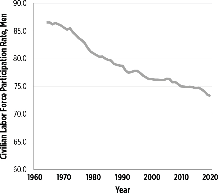
NOTE: Civilian labor force participation rate for men, annual, seasonally adjusted.
SOURCE: U.S. Bureau of Labor Statistics, Civilian Labor Force Participation Rate: Men [LNS11300001], retrieved from FRED, Federal Reserve Bank of St. Louis. Available: https://fred.stlouisfed.org/series/LNS11300001 [April 12, 2018].
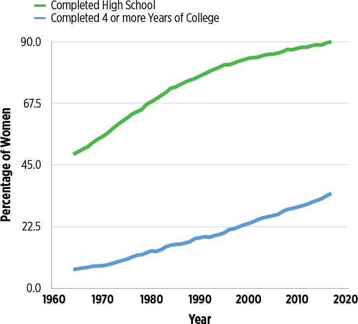
NOTE: Percent of women 25 years and over who have completed high school or college.
SOURCES: Data for 1952 to 2002 from March Current Population Survey; data for 2003 to 2017 from Annual Social and Economic Supplement to the Current Population Survey (noninstitutionalized population, excluding members of the Armed Forces living in barracks); 1950 Census of Population and 1940 Census of Population (resident population).
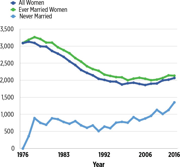
NOTE: Fertility rate for children born per 1,000 women aged 40–44 by marital status from 1976 to 2016. For information on confidentiality protection, sampling error, nonsampling error, and definitions, see the technical documentation available at https://www.census.gov/programs-surveys/cps/technical-documentation.html.
SOURCE: U.S. Census Bureau, Current Population Survey, June 1976–2016.
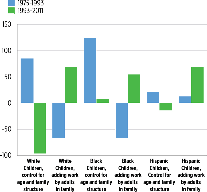
SOURCE: Adapted from Nichols (2013).
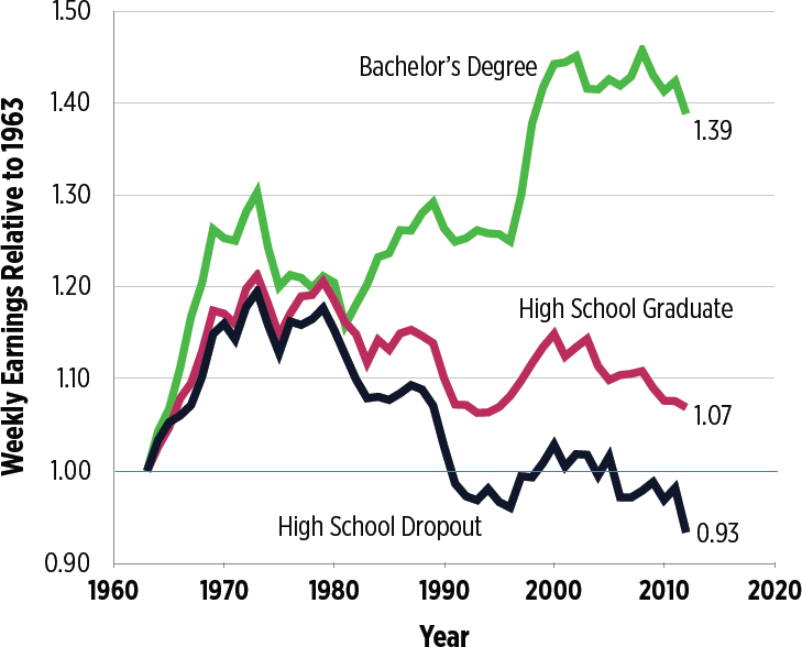
NOTE: Conversion to real 2012 dollars using CPI-U-RS price series.
SOURCE: Autor (2014).
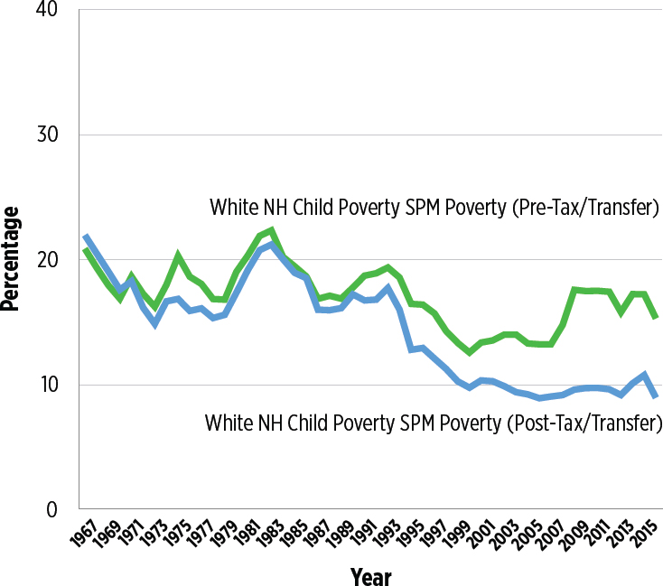
NOTE: “Pretax/Pretransfer” income was calculated by taking the total SPM resources and removing total taxes (tax credits and taxes paid), SNAP, WIC, School Lunch, LIHEAP, housing subsidies, TANF, SSI, Social Security, Unemployment Insurance, and a few smaller government insurance payments such as veteran’s assistance.
SOURCE: Wimer (2017).
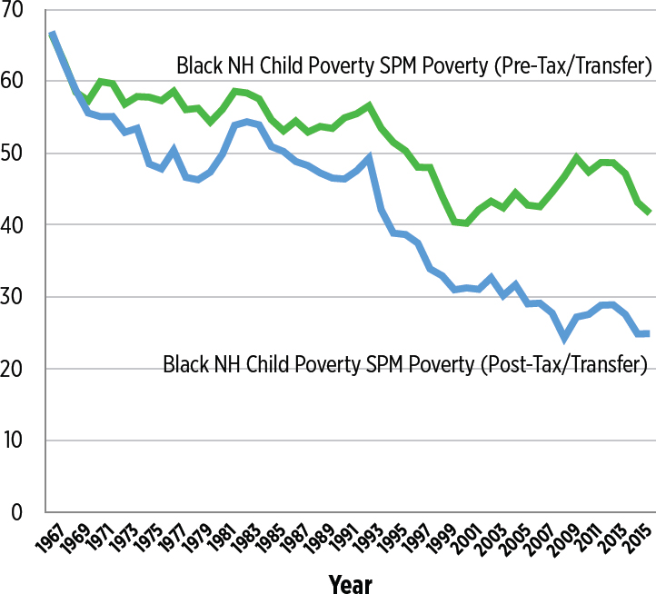
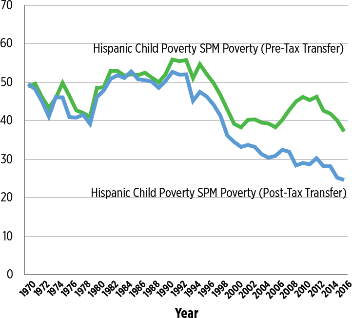
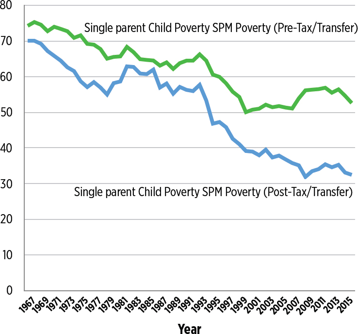
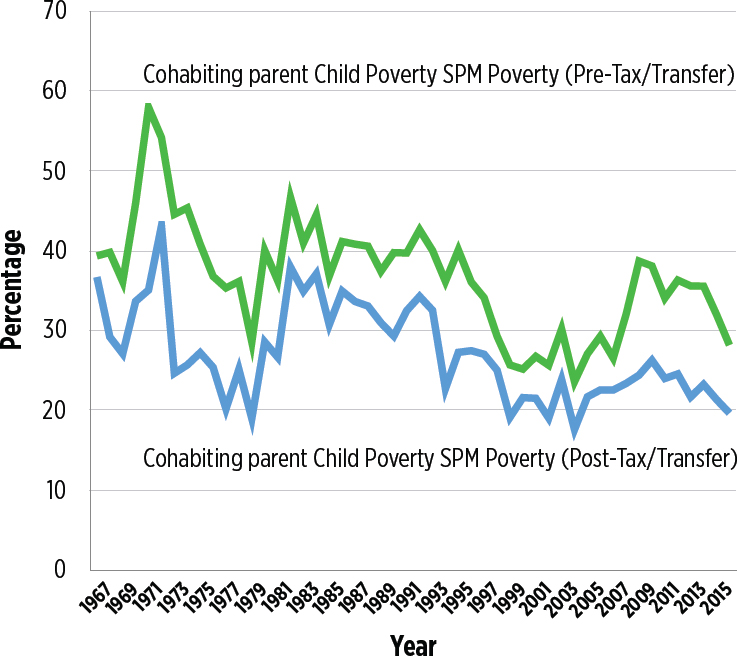
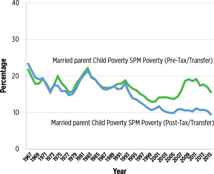
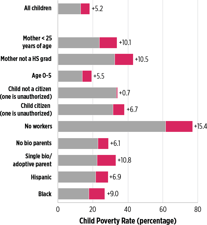
NOTE: Family incomes are adjusted for underreporting.
SOURCE: Estimates from TRIM3 commissioned by the committee.
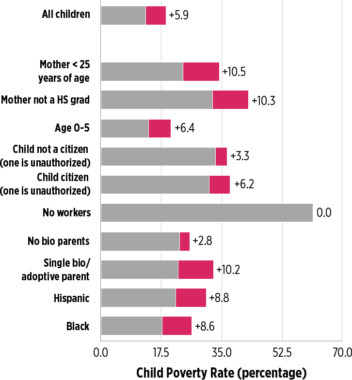
NOTE: Family incomes are adjusted for underreporting.
SOURCE: Estimates from TRIM3 commissioned by the committee.
TABLE D4-1 Federal Expenditures in the United States on Children by Program, Selected Years, 1960–2017 (in billions of 2017 dollars)
| 1960 | 1980 | 2000 | 2010 | 2017 | |
|---|---|---|---|---|---|
| Nutrition | 1.5 | 22.5 | 30.9 | 60.8 | 58.0 |
| SNAP (Food Stamps) | — | 11.7 | 13.4 | 36.1 | 30.6 |
| Child Nutrition | 1.5 | 9.1 | 12.7 | 18.3 | 22.3 |
| WIC | — | 1.6 | 4.8 | 6.4 | 5.0 |
| Income Security | 14.6 | 33.6 | 46.4 | 58.0 | 54.3 |
| Social Security | 7.0 | 17.7 | 18.6 | 22.3 | 20.8 |
| AFDC/TANF | 4.8 | 11.0 | 15.9 | 17.2 | 12.8 |
| Supplemental Security Income | — | 0.9 | 6.7 | 11.0 | 10.5 |
| Veterans Compensation (Disability Compensation) | 2.5 | 3.5 | 2.1 | 3.5 | 6.8 |
| Child Support Enforcement | — | 0.9 | 4.4 | 4.9 | 4.1 |
| Other Income Security | 0.3 | -0.4 | -1.3 | -1.0 | -0.6 |
| Housing | — | 2.8 | 8.3 | 10.7 | 9.5 |
| Section 8 Low-Income Housing Assistance | — | 1.4 | 6.5 | 8.0 | 7.7 |
| Low-Rent Public Housing | — | 0.6 | 1.1 | 1.3 | 1.0 |
| Other Housing | — | 0.8 | 0.8 | 1.4 | 0.7 |
| Refundable Portions Of Tax Credits | — | 3.1 | 34.5 | 81.8 | 74.0 |
| Earned Income Tax Credit | — | 3.1 | 33.3 | 54.8 | 53.1 |
| Child Tax Credit | — | — | 1.1 | 25.4 | 19.4 |
| Premium Tax Credit | — | — | — | — | 0.6 |
| Other Refundable Tax Credits | — | — | — | 1.6 | 0.8 |
| Tax Reductions | 41.2 | 50.1 | 93.1 | 105.1 | 106.2 |
| Dependent Exemption | 40.6 | 42.3 | 39.7 | 36.0 | 37.8 |
| Exclusion for Employer-Sponsored Health Insurance | NA | 4.1 | 13.7 | 21.5 | 22.9 |
| Child Tax Credit (Non-Refundable Portion) | — | — | 26.8 | 33.4 | 29.9 |
| Earned Income Tax Credit (NonRefundable Portion) | — | 1.8 | 5.9 | 5.3 | 7.0 |
| Dependent Care Credit | — | — | 3.2 | 3.8 | 3.3 |
| Other Tax Reductions | 0.7 | 1.9 | 3.7 | 5.1 | 5.3 |
| Health | 0.2 | 7.6 | 36.8 | 95.1 | 111.9 |
| Medicaid | — | 6.9 | 32.8 | 80.7 | 89.9 |
| Chip | — | — | 1.7 | 8.5 | 15.4 |
| Vaccines for Children | — | — | 0.7 | 4.0 | 4.4 |
| Other Health | 0.2 | 0.8 | 1.6 | 1.9 | 2.1 |
NOTE: CHIP = Children’s Health Insurance Program; WIC = Special Supplemental Nutrition Program for Women, Infants, and Children.
SOURCE: Adapted from Isaacs et al. (2018).
TABLE D4-2 Estimated Change in Child Poverty If Current Programs Were Eliminated
| Social Securitya | UC, WC, other | Federal EITC, ACTC | SNAP | Housing Subsidies | SSI | Other benefitsb | |
|---|---|---|---|---|---|---|---|
| Change in number of children by poverty level (thousands) | |||||||
| < 100% | 1,715 | 524 | 4,375 | 3,829 | 1,328 | 1,346 | 1,917 |
| < 50% | 1,095 | 240 | 615 | 2,049 | 300 | 779 | 716 |
| 50% to <100% | 620 | 285 | 3,760 | 1,780 | 1,028 | 568 | 1,201 |
| 100% to <150% | -357 | 80 | -1,311 | -2,361 | -958 | -709 | -514 |
| Percentage point change in children in each poverty range | |||||||
| < 100% | 2.3 | 0.7 | 5.9 | 5.2 | 1.8 | 1.8 | 4.1 |
| < 50% | 1.5 | 0.3 | 0.8 | 2.8 | 0.4 | 1.1 | 1.0 |
| 50% to < 100% | 0.8 | 0.4 | 5.1 | 2.4 | 1.4 | 0.8 | 1.6 |
| 100% to < 150% | -0.5 | 0.1 | -1.8 | -3.2 | -1.3 | -1.0 | -0.7 |
NOTE: ACTC = Additional Child and Dependent Care Tax Credit; EITC = Earned Income Tax Credit; Other = Veterans Benefits (non means-tested), State Temporary Disability Benefits, and Black Lung Miner Benefits; SNAP = Supplemental Nutrition Assistance Program; SSI = Supplemental Security Income; UC = Unemployment Compensation; WC = Worker’s Compensation.
a Social Security includes Social Security Income (including Social Security Retirement, Social Security Disability, Social Security Survivors, and Railroad Retirement).
b Other benefits include Temporary Assistance for Needy Families (TANF), Solely State-Funded Assistance, Other public assistance, means-tested veterans’ benefits, means-tested education assistance, Low Income Home Energy Assistance Program (LIHEAP), National School Lunch Program, and the Special Supplemental Nutrition Program for Women, Infants, and Children (WIC).
SOURCE: Original analyses commissioned by the committee from TRIM3.
APPENDIX D, 5-1
ADJUSTING ESTIMATES OF POVERTY REDUCTION FOR BEHAVIORAL EFFECTS
As discussed at the beginning of Chapter 5, tax and transfer programs may change behaviors in ways that could magnify or moderate program impacts on poverty. Key behaviors involve labor market (employment and hours of work) and family structure choices (marriage and fertility). For example, evidence consistently suggests that the Earned Income Tax Credit (EITC) increases employment and earnings among single mothers (Nichols and Rothstein, 2016). This strong pro-work effect (coupled with little evidence of earnings reduction for those already in the labor market) strengthens the anti-poverty effect of the program over what it would be if family income only increased by the amount of the initial benefit. On the other hand, that benefits phase out at higher income levels in income-tested programs like the Supplemental Nutrition Assistance Program (SNAP), public housing, and the Supplemental Security Income (SSI) program can lead to reductions in employment and/or hours worked. Earning reductions weaken the anti-poverty effects of the programs over what they would be if family income only increased by the amount of the benefit.
A large volume of scholarly research on behavioral effects of policies over the last 40 years has shown that policies can and sometimes do affect employment and hours of work, although the magnitude of the impacts vary across studies and often appear only for some population groups. However, while transfer programs frequently affect the employment and hours of work of their recipients, a given program’s caseload is often too small to change the aggregate poverty rate very much, leading one recent review to conclude that, while there are significant behavioral side effects of many programs, they have little effect on the aggregate poverty impact of the safety net system (Ben-Shalom, Moffitt, and Scholz, 2012). Nevertheless, because behavioral effects on employment and hours of work can be nonnegligible if the caseload is large and if the impact on recipients is significant, the committee’s judgments regarding consensus estimates of these behavioral effects are incorporated in the poverty estimates reported in Chapters 5 and 6. Program-by-program details on our behavioral assumptions are provided in this appendix, with additional implementation details provided in Appendix F.
A smaller research literature attempts to estimate behavioral effects of programs and policies on family structure and childbearing. As described in Chapter 7, estimates from this research are much more tenuous and variable than those for the effects of programs and policies on labor market behavior. More often than not, no statistically significant responses are found. As a result, the committee did not simulate behavioral responses on family structure and childbearing. We refer to this evidence selectively below.
APPENDIX D, 5-2
MODIFICATIONS TO THE EARNED INCOME TAX CREDIT
The committee simulated the impacts of two policy options for the EITC:
EITC Policy #1: Increase payments along the phase-in and flat portions of the EITC schedule.
This option was proposed in Giannarelli et al. (2015) and based on 2011 data. We adapt their proposal to our 2015 data. Specifically, the revised credit would phase in at a greater rate, reach the “plateau” region (where the credit does not increase with earned income) at an earlier point, and begin decreasing the credit at a lower level of income (but at the same marginal tax rate).
EITC Policy #2: Increase payments by 40 percent across the entire schedule, keeping the current earnings eligibility range.
Appendix F provides the details of these two proposed policy changes.
Behavioral Responses to Expanding the EITC
A central feature of the EITC is that it requires earned income to be eligible. The credit is phased in at low earnings levels and then phased out at higher earnings levels. For single earner families, the EITC leads to increases in employment (Eissa and Liebman, 1996; Grogger, 2003; Hoynes and Patel, 2018; Meyer and Rosenbaum, 2000, 2001). The effects are large—the 1993 expansion led to a 7 percentage point increase in employment for low educated single women (Hoynes and Patel, 2018), consistent with the high subsidy rate in the phase-in region of the credit (40% for single parents with two or more children).
The credit is predicted to reduce labor supply for those in the labor market for all but the lowest-earning single parent workers (e.g., those in the phase-in region have negative income effects but positive substitution effects). However, there is little empirical support for this prediction other than some evidence that self-employed workers adjust to maximize the credit along the phase-in region (Chetty, Friedman, and Saez, 2013; Chetty and Saez, 2013; Saez, 2010). Theory is more complicated for two earner couples, but we expect secondary earners to reduce work effort at the extensive (employment) and intensive margin (hours of work) of labor supply. The research shows small reductions in employment and intensive margin responses for secondary earners and little effect on primary earners (Eissa and Hoynes, 2004, 2006).
The EITC may affect pretax wages. To the extent that the EITC increases labor force participation, tax incidence models suggest that the earnings subsidy in the EITC will be shared between the employers and employees. The implication is a reduction in the pretax wage, allowing employers of EITC recipients to capture a portion of the money spent on the EITC. There is limited evidence on the magnitude of the wage effects (Leigh, 2010; Rothstein, 2008, 2010) yet a recent review concluded “Although none of the evidence is airtight, it appears that employers of low-wage labor capture a meaningful share of the credit through reduced wages and that this comes to some extent at the expense of low-skill workers who are not eligible for the credit (due, e.g., to not having children)” (Hoynes and Rothstein, 2017, p. 214).
The EITC also creates incentives for low-income one-earner couples to marry and creates incentives for low-income two-earner couples to avoid marriage or separate. Therefore, the EITC, like ordinary income taxes, creates marriage penalties for some and marriages bonuses for others; these incentives are inherent in a family-based tax system. Because the credits increase with the number of children, they may incentivize additional births. For marriage, the evidence is largely inconclusive and any effects appear to be quite small (Ellwood, 2000; Herbst, 2011; Michelmore, 2018; Rosenbaum, 2000). There is less evidence on the effects of the EITC on fertility (Baughman and Dickert-Conlin, 2009) but again the results suggest small effects.
To incorporate behavioral adjustments into the TRIM3 model, we start by identifying estimates from the literature. Based on the research papers we have referenced above, we make the following assumptions:
- Single mothers / Extensive margin: We assume that a $1,000 in EITC payments (in 2013 dollars) will generate a 7 percent (5.6 percentage point) increase in employment for women with some college or less (all education groups). [Source: Hoynes and Patel, 2018]
- Single mothers / Intensive margin: We assume no adjustment in hours or earnings.
- Single fathers: We assume no adjustment of labor supply.
- Married couples / Extensive margin: We assume that there is no adjustment for married men and that the magnitude of the 1984–1996 increase in the EITC leads to a 1.1 percentage point reduction in employment for married women. [Source: Eissa and Hoynes, 2004]
- Married couples / Intensive margin: We assume that there is no adjustment for married men and that the magnitude of the 1984–1996 increase in the EITC leads to a 46 annual hours reduction in employment for married women. [Source: Eissa and Hoynes, 2004]
TABLE D5-1 Behavioral Assumptions for the Two EITC Policy Options
| Single Mother Extensive Margin | Married Mother Extensive Margin | Married Mother Intensive Margin | |
|---|---|---|---|
| Policy #1: Increase Payments Along Phase-in and Flat Portions of the EITC Schedule | +3 ppt | No Change | No Change |
| Policy #2: Increase Payments by 40% Across the Entire Schedule | 4 Times Policy A | 4 Times Policy A | 4 Times Policy A |
Given these estimates from the literature, Table D5-1, shows the behavioral assumptions that we implement in TRIM3, for each of the policy simulations. Appendix F provides the details of how these assumptions about the magnitude of the behavioral response are implemented in TRIM3.
The employment effects of both EITC-based policies are large. Policy #1 results in an additional 270,000 workers in the economy and is estimated to increase aggregate earnings by $4.9 billion.41 Policy #2 generates a net increase of 541,000 workers and an earnings increase of $9.0 billion. These effects constitute a significant contribution to the poverty reduction of the policies. Policy #1 reduces child poverty from 13.0 percent to 12.2 percent without employment effects but down to 11.8 percent with those effects; for Policy #2, the reduction is to 12.1 percent without employment effects but 10.9 percent with them.
___________________
41 As with all of the policy simulations in the report, data on earnings and employment changes are restricted to individuals living in families with incomes below 200 percent of the SPM poverty thresholds.
APPENDIX D, 5-3
MODIFICATIONS TO CHILD CARE SUBSIDIES
The committee simulated the impacts of two policy options for expanding child care subsidies.
Child Care Policy #1: Convert the Child and Dependent Care Tax Credit (CDCTC) to a fully refundable tax credit and concentrate its benefits on families with the lowest incomes and with children under the age of 5.
This policy proposal expands the CDCTC along the lines suggested by Ziliak (2017) in his memo to the committee. Specifically, it would:
- Convert the CDCTC from a nonrefundable credit to a refundable credit;
- Cap the eligibility for CDCTC at $70,000;
- Make the CDCTC credit a progressive function of adjusted gross income (AGI) and age of child (based on the fact that the cost of child care is higher for infants and toddlers than older children). For families with children under the age of 5 and an AGI less than or equal to $25,000, the credit rate would be 100 percent up to $4,000 in qualifying child care expenses for the first child, with maximum allowable expenses of $6,000 for two or more children. The credit rate declines by 10 percent for each additional $5,000 in AGI, and is set to zero for an AGI above $70,000. For families with children ages 5-12, the credit rate would be 70 percent for families with an AGI below $25,000 and decline by 7 percent for each additional $5,000 in AGI above $25,000; and
- Keep the definition of “qualifying child care expenses” the same as current policy; both formal and informal child care expenses would qualify if the child care provider has a tax identification number.
The ceilings for qualifying child care expenses stipulated above derive from two sources: (1) Ziliak’s (2014) calculations of data on out-of-pocket child care costs pooled across the 2012–2013 waves of the Current Population Survey, and (2) estimates of child care costs from the National Association of Child Care Resource and Referral Agencies. Calculations based on the Current Population Survey indicated that for single working mothers with a child under age 5, median family earnings was $19,200 and median out-of-pocket child care costs was $3,000, with an interquartile range of $4,400 in out-of-pocket child care costs (interquartile range is the difference between the 75th percentile and the 25th percentile of out-of-pocket child care costs). For single working mothers with a child under age 13, median
family earnings was $23,088 and median out-of-pocket child care costs was $2,600, with an interquartile range of $3,800.42
Child Care Policy #2: Guarantee assistance from the Child Care and Development Fund (CCDF) for all eligible families with incomes below 150 percent of the poverty line.
This policy option was proposed in Giannarelli et al. (2015) and would expand CCDF subsidies to guarantee assistance for all eligible families with incomes below 150 percent of poverty who want subsidies, with no limitations based on available funds (Giannarelli et al., 2015). States that currently use an income limit for child care subsidies that is higher than 150 percent of poverty were assumed to continue using those higher limits. This option does not include any changes to the states’ other eligibility policies—such as the definition of family units—or to the states’ methods for computing copayments.
Behavioral Responses to Expanding Child Care Subsidies
A large body of research indicates that government child care subsidy programs increase employment rates among mothers in low-income families. Blau (2003) and Blau and Tekin (2007) report findings from several local-area reforms in the 1980s and early 1990s showing positive impacts on employment. Studies of the impact of the CCDF, one of the programs in our proposal, have also been conducted or reviewed by Blau and Tekin (2007), Fang and Keane (2004), and Tekin (2007). The CCDF was found to increase employment of single mothers by 0.1 to 1.3 percentage points between 1997 and 2002 in one study and by a much larger 13 percentage points in another.
We base our estimated employment responses to both the CDCTC and the CCDF on a review by Blau (2003) of the general impacts of child care subsidies on maternal labor supply. Blau reviewed a large number of studies that had provided estimates of the elasticity of employment with respect to a change in the net hourly cost of child care (the latter defined as the out-of-pocket cost of care per hour of work). The studies he reviewed showed elasticities ranging from -0.34 to 0.07. We take the midpoint of this range, equal to -0.20, implying that a 10 percent reduction in the hourly cost of child care will increase the employment rate by 2 percent. We apply this elasticity to the percentage decrease in aggregate out-of-pocket child care spending due to the policy change to compute the targeted employment
___________________
42 See http://www.hamiltonproject.org/assets/legacy/files/downloads_and_links/child_care_credit_ziliak.pdf.
increase. The additional employment is then distributed randomly across women who, if they began to work, would benefit from the policy. Further implementation details can be found in Appendix F. The research literature focuses almost exclusively on the impacts of child care costs on employment rather than on hours of work conditional on employment. We therefore lacked sufficient research evidence to simulate effects at the intensive margin.
Both policy options have significant impacts on employment and earnings and these are responsible for essentially all of the poverty reduction. Child Care Policy #1 results in an additional 518,000 low-income workers in the economy and a net earnings increase in the economy is $9.3 billion. Child Care Policy #2 generates an additional 236,000 low-income workers and an aggregate net earnings increase of $4.2 billion. In the absence of any employment effects, the two policy options reduce child poverty from its initial 13.0 percent level to 12.7 percent and 12.9 percent, respectively. The employment effects reduce these rates down to the 11.8 percent and 12.4 percent reported in the text.
APPENDIX D, 5-4
MODIFICATIONS TO THE MINIMUM WAGE
The committee simulated two increases in the federal minimum wage:
Minimum Wage Policy #1: Raise the current $7.25 per hour federal minimum wage to $10.25 (moving from current level in 3 years 2017-2020) and index it to inflation after that.
Minimum Wage Policy #2: Raise the federal minimum wage to $10.25 or the 10th percentile of the state’s hourly wage distribution, whichever is lower, and index it to inflation after that.
Policy #1 imposes this increase in all states. The $10.25 amount for 2020 is recommended in order not to disrupt the labor market in low wage states as measured by their wages at the 25th percentile of the wage distribution. It is similar to but below the Congressional Budget Office’s (CBO’s) (2014) and Sawhill and Karpilow’s (2014) proposed minimum wage of $10.10 for 2017. Policy #2 follows Dube (2014), who recommends setting minimum wages to take account of local prevailing wages. We note below that all states have minimums below the 25th percentile of their wage distribution and that that percentile of their wage distribution is above the proposed $10.25 minimum wage for 2015 and 2016. But the 2015 and 2016 10th percentile wages would be affected in many states; hence the
second simulation showed some increase from the $7.25 federal minimum wage, but a lesser increase in low wage states.43
The implementation of the increases follows the methodology of the CBO (2014) as closely as possible. For example, a tolerance of 25 cents below the minimum wage is used to identify individuals in the Current Population Survey who report a wage slightly below the minimum but who may have simply been misreporting. They are considered to be paid the minimum wage. Also, the CBO models a ripple effect of an increase in the minimum wage for workers above the new minimum, with the assumption that the wages of workers up to 50 percent more than the minimum wage also increase. Separate tipped minimum wages were assumed for tipped workers, and their minimums were increased by the same amounts as the overall minimums. More implementation details can be found in Appendix F.
Behavioral Responses to Raising the Minimum Wage
By raising the cost of labor, increases in the minimum wage are expected to reduce employment (while raising earnings for those receiving the minimum wage). For modeling this behavioral adjustment of the increase in the minimum wage, we again follow CBO (2014) as closely as possible. The CBO considered -0.075 for teenagers as a best estimate of the employment elasticity with respect to an increase in the minimum wage. This implies that a 10 percent increase in the minimum wage would reduce teen employment by 0.75 percent. CBO divided this elasticity by the fraction of teenagers who are likely be affected by the minimum wage increase, which they estimated to be one-third. This generates an elasticity of -0.225 for those teenagers actually affected. The CBO then adjusted the elasticity upward by 50 percent of its value because the change in actual wages was typically about that percent greater than the wage change that was necessary for compliance with the new minimum wage. The resulting elasticity for teenagers is -0.3375.
The CBO assumed the elasticity for adults would be one-third of that, or -0.1125. In its simulations, the TRIM3 model was used to calculate employment effects for each person in the model, using the actual change in wages for each individual and multiplying those by the relevant elasticities. No employment losses were assumed to occur for the spillover group. The
___________________
43 The Bureau of Labor Statistics (BLS) Occupational Employment and Wage Statistics series has the 10th percentile of the wage distribution by state. See https://www.bls.gov/oes/2015/may/oessrcst.htm for the 2015 data. A summary of the statistics for other years has been compiled from BLS data by http://www.governing.com/gov-data/wage-average-median-paydata-for-states.html.
TRIM simulation indicated that 28 percent of families with children with incomes under 200 percent Supplemental Poverty Measure (SPM) poverty had at least one worker who was affected by the minimum wages. Simulations of the first policy show a loss of 42,000 jobs among individuals living in families with incomes below 200 percent of SPM poverty. The net increase in earnings for those who continued to work is $3.5 billion.44 For the second policy, 28,000 jobs were lost and net earnings increased by $1.9 billion.
APPENDIX D, 5-5
SCALING UP WORKADVANCE
Based on an MDRC program evaluation (Hendra et al., 2016), the committee simulated the impacts of two policy options involving WorkAdvance.
WorkAdvance Policy #1: All men heading families with children and income below 200 percent of the poverty line would be eligible for WorkAdvance programming and training slots would be created for 10 percent of them.
WorkAdvance Policy #2: All men heading families with children and income below 200 percent of the poverty line would be eligible for WorkAdvance programming and training slots would be created for 30 percent of them.
We begin by restating a point made in Chapter 5: The evaluations of WorkAdvance enrolled men in all four of the evaluation sites but significant numbers of women in only one of them. Consequently, we considered results for women to be too statistically unreliable. We have no evidence-based reason to want to limit the program options for men but were forced to do so owing to the nature of the evidence. Also, our use of the term family “head” refers to individuals the U.S. Census Bureau defines as “householder” or spouses of “householders.”
The 10 percent and 30 percent scale-up assumptions in our two policy proposals would both lead to large programs (487,000 and 1,464,000 enrollees, respectively, for the two programs) compared with the 2,564 enrollees in the MDRC experiment (Hendra et al., 2016) but still considerably less than the numbers of families affected by our other proposals.
___________________
44 As might be expected, both job losses and net earnings changes are several times larger than these amounts in simulations based on the entire population as opposed to just those individuals living in families with incomes below 200 percent of SPM poverty. Of all of the program and policy options we consider, our minimum wage proposals are least targeted to children living below or near the poverty line.
Nevertheless, the difference in impacts for our two proposals provides a sense of how the poverty impact would vary with program size. The enrollees in the MDRC experiment also had higher levels of education than the average in the population because a minimal level of skills was judged necessary to make the training program effective—56 percent of the MDRC study enrollees had at least some college and 44 percent had a high school degree or less. The proportions of enrollees simulated to receive training were therefore adjusted to meet this ratio. Our proposals therefore affect a more highly skilled population, with higher earnings, than most of our other policies.
The MDRC experimental results showed an average impact across all four sites of $1,900 per year in 2015 dollars, but the impacts varied by initial employment status. Those unemployed for 7 or more months experienced a gain of $1,933, those unemployed for 1 to 6 months experienced a gain of $3,112, and those unemployed for less than 1 month or who were employed experienced a loss of $327. The Current Population Survey data on which the TRIM3 model is based has information on the employment status of individuals and the length of time they have been unemployed, so the simulated earnings impacts were conducted separately for each of these three groups. The MDRC experiment enrolled participants in the three employment-status groups in these rough proportions: 40 percent, 30 percent, and 30 percent, respectively. The simulations selected men for the program in these same proportions.
Behavioral Responses to WorkAdvance
The nature of the program is such that no behavioral responses need be simulated on top of the direct creation of additional earnings. The simulation simply randomly selects men in the eligible category and in the proportions noted above, and assigns them the earnings levels just noted. The number of enrollees in the 10 percent and 30 percent programs is simulated to be 487,000 and 1,464,000, respectively. Aggregate earnings increase by $817 million per year for the first program and by $2.4 billion for the second. The direct administrative cost is $2.99 billion and $8.99 billion, respectively, for the two programs, but the increased earnings of enrollees results in additional tax revenues and reduced benefits from other programs, for savings of $271 million for the first program and $801 million for the second program.45 The resulting net costs are $2.72 billion and $8.19 billion, respectively.
___________________
45 MDRC reports the direct administrative cost of WorkAdvance as $5,950 per enrollee in 2012 dollars, or $6,142 in 2015 CPI-U dollars.
APPENDIX D, 5-6
MODIFICATIONS TO THE SUPPLEMENTAL NUTRITION ASSISTANCE PROGRAM (SNAP)
The committee simulated two SNAP policy options:
SNAP Policy #1: Increase SNAP benefits by 20 percent and make adjustments for the number of children greater than or equal to 12 years of age in the home ($360 more per each teenager per year) plus Summer Electronic Benefit Transfer for Children (SEBTC) ($180 more per child in pre-kindergarten through 12th grade per year).
SNAP Policy #2: Increase SNAP benefits by 30 percent and make adjustments for the number of children greater than or equal to 12 years of age in the home ($360 more per each teenager per year) plus Summer Electronic Benefit Transfer for Children (SEBTC) ($180 more per child in pre-kindergarten through 12th grade per year).
Both the general benefit increase and the teen adjustment were implemented by increasing the Thrifty Food Plan (TFP) allotments by these amounts.
In formulating these options, the committee reviewed memos received from several experts and used these as the basis for formulating its policy options that were simulated using the TRIM3 model (Allen, 2017; Sherman, 2017; Ziliak, 2017). The first two memos recommended that the SNAP benefit, currently set at the U.S. Department of Agriculture’s (USDA’s) TFP level, be increased to the USDA’s Low-Cost Food Plan level, a 30 percent increase, which Allen and Sherman estimate to reduce poverty by 16 percent. For a family of three, this would amount to an increase of about $1,896 per year in SNAP benefits, according to Sherman (2017). Ziliak (2017) proposed a 20 percent increase, based on a completely different rationale. He argued that the TFP does not take into account the amount of time necessary for food preparation. Ziliak cites research indicating that 13 to 16 hours per week of food preparation time is needed to achieve the TFP, which is impossible for adults who are working full time and, in fact, almost no parents currently spend anywhere close to that amount of time in food preparation. Adults who work must instead economize on their time and purchase more expensive food. He cites research that valued the time that must be given up to prepare food at the hourly wage rate; the results suggest about a 20 percent increase in the SNAP benefit.
Another issue examined in the policy simulations was an adjustment to SNAP benefits to account for the age of the children in the home. Currently, SNAP benefits do not account for the age of children (USDA assumes, for the TFP calculation, that there are two children under the age of 12
in the home). Ziliak (2017) mentions this as an issue, noting that dietary requirements for teenagers are almost as high as those for adults. Further, food insecurity has been repeatedly shown to be higher among families with teenagers (Nord, 2009). Anderson and Butcher (2016) demonstrated that families with teenagers have higher unmet food needs and suggested that an additional $30 SNAP benefit per month per capita would eliminate that need.
A third issue that the committee considered was the addition of the Summer Electronic Benefit Transfer for Children (SEBTC). This benefit is designed to address food gaps for children during the summer when they lack access to school-based food assistance programs. USDA has piloted this in five states, in three of which benefits were distributed via the SNAP model. In 2013, they used an experimental design to test two levels of support, $60 or $30 per month per child in pre-kindergarten through 12th grade. The $60 per month amount was found to reduce very low food security for children by 26 percent and also helped improve food security for the entire family. The $30 per month amount yielded similar impacts on children, but was less effective for the household (Collins et al., 2016).
TRIM3 Implementation
The implementation of the increase in SNAP benefits and the increase in the teen increment in the TRIM3 model was implemented by increasing the TFP allotment. This increases benefits for SNAP recipients at all income levels and also increases the income eligibility point in SNAP, although only in cases where the maximum income limit was not hit first. All other features of the SNAP benefit formula were left unchanged. The TRIM3 model has a participation equation which predicts how many eligible families participate in the program as a function of the benefit level and family characteristics. This equation was used to simulate families who would begin to receive program benefits after the benefit increase. For the SEBTC, since all children participating in the School Breakfast Program (SBP) or National School Lunch Program (NLSP) are eligible for SEBTC, and since SNAP receipt makes a family eligible for SBP or NLSP, SNAP receipt was used as the criterion for receiving the SEBTC. An SEBTC of $60 was added as a lump sum to the SNAP benefit for each of the three summer months a family with a child in school received SNAP. Since the SEBTC is also provided to children in pre-school, those families were also simulated to receive SEBTC, using a 40 percent takeup rate for 3-year-olds in poor families, a 50 percent takeup rate for 4-year-olds in poor families, a 35 percent takeup rate for nonpoor families with 4-year-olds, and a 66 percent takeup rate for families with a 5-year-old (all based on studies of preschool enrollment rates of children of different ages and poverty statuses).
Behavioral Responses to Expanding SNAP
A handful of studies estimate the effects of the SNAP program and its predecessor, the Food Stamp Program, on employment, earnings, and labor supply (see reviews by Currie, 2003; Hoynes and Schanzenbach, 2016). Most studies have found very modest negative effects of the program, possibly because the rate at which benefits are phased out as income increases (30%) is fairly modest. We rely on the estimates of Hoynes and Schanzenbach (2012) which used the rollout of the Food Stamp Program in the 1970s to assess the effects of the program on work effort. Those authors found that the program reduced the employment rate of single mothers from 11 to 27 percentage points, with a midpoint estimate of 19 percentage points. They also found a reduction in annual hours of work from 281 to 505, with a midpoint of 393. The 20 percent increase in benefits in the committee’s proposal is about one-fifth of the rollout benefit increase, which would amount to a 3.8 percentage point reduction in employment and a reduction in annual hours of 78.6. Because the rollout is relatively old and occurred when there were few other programs, we posit a lower bound estimate of 1 percentage point reduction in employment and a 50-hour reduction in annual hours. For cost reasons, we conduct only one simulation and use the midpoint of our upper and lower bound estimates for single mothers, for a 2.4 percentage point reduction in employment and a 64.3 reduction in annual hours. For single mothers made newly eligible for SNAP because of the higher income eligibility level (and hence lower benefits), we assume no employment reduction but a 25-hour-per-year hours reduction.
There is much less research on effects of the program on work effort of married men and married women with children. We assume no employment reduction for men and an upper bound of 0.5 percentage point reduction employment for married women, with a lower bound of 0 and hence an average of 0.25 percentage points. We assume no response for those made newly eligible.
The simulations show a reduction of 139,000 workers for the first SNAP reform and 157,000 for the second. The aggregate earnings reduction is $3.2 billion for the first SNAP reform and $3.6 billion for the second. Benefits increase modestly from other programs but the main cost of the reforms is the direct cost of additional SNAP benefits. The child poverty rate after implementation of the first policy would have been 11.0 percent in the absence of employment effects instead of the 11.3 percent we report in the text. For the second policy, the rate would have been 10.4 percent instead of the 10.7 percent we report.
APPENDIX D, 5-7
MODIFICATIONS TO HOUSING PROGRAMS
The committee simulated two expansions of the Housing Choice Voucher Program, both aimed at increasing the share of eligible families that are able to access and use the vouchers.
Housing Voucher Policy #1: Increase the number of vouchers directed to families with children so that 50 percent of eligible families not currently receiving subsidized housing would use them.
Housing Voucher Policy #2: Increase the number of vouchers directed to families with children so that 70 percent of eligible families not currently receiving subsidized housing would use them.
The TRIM3 model uses estimates of income eligibility in local areas to determine who is eligible for voucher programs, and then applies an approximate rent formula to determine how much the household pays in rent. It identifies who currently resides in subsidized housing programs from questions asked in the Current Population Survey. The simulations for the expansion of vouchers were conducted by randomly selecting either 50 percent or 70 percent of all families eligible for vouchers but not currently receiving them, and assigning those randomly selected a housing unit.
A drawback of the TRIM3 model for subsidized housing program participation is that it relies on a small number of questions on the Current Population Survey that have significant error and do not accurately identify the type of subsidized housing program in which the respondent participates. There are dozens of local and federal housing programs in addition to the best known and largest three, discussed in Chapter 5. When responses to questions on the American Housing Survey are matched to administrative data from the U.S. Department of Housing and Urban Development (HUD) from program records, it is apparent that there are significant reporting errors. In particular, participation in housing voucher and public housing programs is underreported, and significant overreporting occurs as respondents say they are in those housing programs but are really in different housing programs.46 The committee had neither the time nor the resources to improve the accuracy of the Current Population Survey questions (e.g., by matching to HUD administrative records or by statistical imputation).
___________________
46 Personal communication from Dr. Edgar Olsen to the committee (September 2017).
Background to the Policy Proposals
Several of the memos the committee received suggested that housing policy reforms had the potential to reduce child poverty. For instance, Olsen (2017) proposed to increase the number of vouchers, funded either by new expenditure or by reductions in the Low-Income Housing Tax Credit (LIHTC), with the option of making the new vouchers go either to all families or just to those with children. He also suggested reducing the generosity of individual vouchers and increasing their number for revenue neutrality. Desmond (2016) recommended expanding public housing, vouchers, or LIHTC, with the second being lowest cost, and he also recommended emergency rental assistance to reduce evictions, publicly-funded legal representation for renters in housing court, and joint programs with schools to ensure that children in subsidized housing attend school. Allen (2017) recommended the Children’s Defense Fund proposal to make housing vouchers universally available to all families with income less than 150 percent of the poverty line (in all areas, independent of median income, which is currently used for local eligibility) and to those who live in areas where the Fair Market Rent (FMR) is more than 50 percent of their family income. They assumed a 70 percent takeup rate among newly eligible families and their simulations showed a 21 percent reduction in child poverty (from 14.6% to 11.5%) for about $23 billion. Sherman (2017) also recommended the Children’s Defense Fund plan, plus a proposal from the Bipartisan Policy Center’s Housing Commission that recommended making vouchers available to all households with incomes at or below 30 percent of the area median income (which, on average, is roughly equal to the poverty line). Heymann and Sprague (2017) proposed extending the mortgage interest rate deduction in the federal income tax to renters, making it refundable, and making it a flat percent independent of income bracket.
Behavioral Responses to Expanding Housing Programs
As with other programs, most research on the behavioral effects of subsidized housing programs has concerned their impact on employment and earnings. A particularly strong research design was used by Jacob and Ludwig (2012), who made use of an expansion of housing vouchers in Chicago where those on the waiting list were randomly offered a voucher. Comparisons of the earnings levels of those in the experimental group to those in the control group showed employment and earnings reductions that sometimes differed by gender and headship status. Based on their results, we assumed no employment response for male heads but a 3.3 percentage point reduction in the employment rate for female heads and married women, and a 7.3 percent reduction in annual hours for all heads and spouses regardless
of gender, for those in the labor market. These effects were applied to those families simulated to be new voucher recipients, and who have children in the household, were under 65, were not disabled, and were not students.
The TRIM3 simulations showed that about 66,000 individuals transitioned from employment to nonemployment for the 50 percent program (Housing Voucher Policy #1) and about 93,000 for the 70 percent program (Housing Voucher Policy #2). Aggregate earnings losses were estimated to total $4.1 billion and $5.9 billion, respectively. On the cost side, the earnings reductions generated increases in benefits from other programs and therefore costs (except for the EITC and child care subsidies, which were reduced and therefore resulted in government cost savings), but the cost changes induced by these indirect changes were extremely small relative to the direct cost (or benefit from the perspective of the recipients) of the new housing subsidies. The impact on poverty rates of the employment effects were modest, for the child poverty rate after implementation of Housing Voucher Policy #1 would have been 10.8 percent in the absence of employment effects instead of the 10.9 percent we report in Chapter 5, whereas for Housing Voucher Policy #2, the rate would have been 9.8 percent instead of the 10.1 percent we report.
APPENDIX D, 5-8
MODIFICATIONS TO THE SUPPLEMENTAL SECURITY INCOME (SSI) PROGRAM
We propose two child-focused modifications to the SSI program, both of which involve increasing child benefit levels:
SSI Policy #1: Increase by one-third the maximum child SSI benefit (to $977 per month from a current baseline of $733).
SSI Policy #2: Increase by two-thirds the maximum child SSI benefit (to $1,222) from a current baseline of $733).
Implementation of these proposals in the TRIM3 model is discussed in Appendix F. Child disability is not identified in the Current Population Survey but family receipt of SSI and the presence of children are both identified. All families with children receiving SSI are selected for this proposal implementation.47 The proposal raises the SSI guarantee, called the Federal Benefit Rate (FBR) in program regulations. Benefits in the program are calculated as the FBR minus countable income, where countable income
___________________
47 For a listing of the diagnoses that qualify an individual for SSI, see Appendix D, Table D5-2.
TABLE D5-2 Recipients Under Age 18, by Diagnostic Group and Age, December 2016
| Diagnostic Group | All Ages | Under 3 | 3-5 | 6-12 | 13-17 |
|---|---|---|---|---|---|
| Number | |||||
| All Recipients Under Age 18 | 1,213,079 | 73,451 | 147,092 | 559,027 | 433,509 |
| Congenital Anomalies | 66,646 | 12,993 | 14,029 | 26,349 | 13,275 |
| Endocrine, Nutritional, and Metabolic Diseases | 9,114 | 593 | 1,862 | 4,264 | 2,395 |
| Infectious and Parasitic Diseases | 699 | 28 | 71 | 302 | 298 |
| Injuries | 5,800 | 495 | 940 | 2,570 | 1,795 |
| Mental Disorders | |||||
| Autistic Disorders | 174,866 | 1,782 | 26,682 | 96,311 | 50,091 |
| Developmental Disorders | 239,215 | 4,686 | 43,040 | 124,954 | 66,535 |
| Childhood and Adolescent Disorders Not Elsewhere Classified | 233,490 | 46 | 3,849 | 117,581 | 112,014 |
| Intellectual Disability | 117,646 | 472 | 4,376 | 46,979 | 65,819 |
| Mood Disorders | 38,412 | 6 | 238 | 11,338 | 26,830 |
| Organic Mental Disorders | 27,211 | 803 | 4,229 | 13,024 | 9,155 |
| Schizophrenic and Other Psychotic Disorders | 3,058 | 0 | 11 | 747 | 2,300 |
| Other Mental Disorders | 31,318 | 56 | 747 | 13,094 | 17,421 |
| Neoplasms | 10,886 | 777 | 2,316 | 4,955 | 2,838 |
| Diseases of the— | |||||
| Blood and Blood-forming Organs | 11,557 | 395 | 1,610 | 5,726 | 3,826 |
| Circulatory System | 4,405 | 627 | 836 | 1,699 | 1,243 |
| Digestive System | 15,408 | 5,123 | 4,771 | 3,927 | 1,587 |
| Genitourinary System | 2,945 | 226 | 425 | 1,230 | 1,064 |
| Musculoskeletal System and Connective Tissue | 9,456 | 783 | 1,618 | 3,840 | 3,215 |
| Nervous System and Sense Organs | 95,835 | 5,590 | 15,117 | 45,594 | 29,534 |
| Respiratory System | 24,437 | 1,889 | 4,665 | 11,130 | 6,753 |
| Skin and Subcutaneous Tissue | 2,309 | 131 | 377 | 1,195 | 606 |
| Other | 74,818 | 34,807 | 13,397 | 16,104 | 10,510 |
| Unknown | 13,548 | 1,143 | 1,886 | 6,114 | 4,405 |
| Diagnostic Group | All Ages | Under 3 | 3-5 | 6-12 | 13-17 |
|---|---|---|---|---|---|
| Percent | |||||
| All Recipients Under Age 18 | 100.0 | 100.0 | 100.0 | 100.0 | 100.0 |
| Congenital Anomalies | 5.5 | 17.7 | 9.5 | 4.7 | 3.1 |
| Endocrine, Nutritional, and Metabolic Diseases | 0.8 | 0.8 | 1.3 | 0.8 | 0.6 |
| Infectious and Parasitic Diseases | 0.1 | (L) | (L) | 0.1 | 0.1 |
| Injuries | 0.5 | 0.7 | 0.6 | 0.5 | 0.4 |
| Mental Disorders | |||||
| Autistic Disorders | 14.4 | 2.4 | 18.1 | 17.2 | 11.6 |
| Developmental disorders | 19.7 | 6.4 | 29.3 | 22.4 | 15.3 |
| Childhood and Adolescent Disorders Not Elsewhere Classified | 19.2 | 0.1 | 2.6 | 21.0 | 25.8 |
| Intellectual Disability | 9.7 | 0.6 | 3.0 | 8.4 | 15.2 |
| Mood Disorders | 3.2 | (L) | 0.2 | 2.0 | 6.2 |
| Organic Mental Disorders | 2.2 | 1.1 | 2.9 | 2.3 | 2.1 |
| Schizophrenic and Other Psychotic Disorders | 0.3 | 0.0 | (L) | 0.1 | 0.5 |
| Other Mental Disorders | 2.6 | 0.1 | 0.5 | 2.3 | 4.0 |
| Neoplasms | 0.9 | 1.1 | 1.6 | 0.9 | 0.7 |
| Diseases of the— | |||||
| Blood and Blood-forming Organs | 1.0 | 0.5 | 1.1 | 1.0 | 0.9 |
| Circulatory System | 0.4 | 0.9 | 0.6 | 0.3 | 0.3 |
| Digestive System | 1.3 | 7.0 | 3.2 | 0.7 | 0.4 |
| Genitourinary System | 0.2 | 0.3 | 0.3 | 0.2 | 0.2 |
| Musculoskeletal System and Connective Tissue | 0.8 | 1.1 | 1.1 | 0.7 | 0.7 |
| Nervous System and Sense Organs | 7.9 | 7.6 | 10.3 | 8.2 | 6.8 |
| Respiratory System | 2.0 | 2.6 | 3.2 | 2.0 | 1.6 |
| Skin and Subcutaneous Tissue | 0.2 | 0.2 | 0.3 | 0.2 | 0.1 |
| Other | 6.2 | 47.4 | 9.1 | 2.9 | 2.4 |
| Unknown | 1.1 | 1.6 | 1.3 | 1.1 | 1.0 |
NOTE: (L) = less than 0.05 percent.
SOURCE: Social Security Administration, Supplemental Security Record, 100 percent data.
is family income after a number of exclusions and deductions, including a general deduction of 50 percent of earned income in the family (adults and children).
An increase in take-up among eligible families (defined as those with children but with income below the SSI eligibility point) of 5 and 10 percentage points for the two respective proposals is assumed, based on calculations from the American Community Survey (which does have a child disability question as well as family income) of a current participation rate of 66 percent among children with a disability combined with the fraction of all children with a disability. Finally, we assume additional participation from families made newly eligible by the increase in the FBR, since our proposals raise the income eligibility point. An increase of 5 percentage points among those made newly eligible is assumed (the number of families made newly eligible is higher in the second policy than in the first).
Behavioral Responses to Expanding Child SSI Benefits
We use the review of behavioral responses by Duggan, Kearney, and Rennane (2016) and a study by Deshpande (2016) to assess work and employment responses to the SSI program. Since almost all SSI children, including teenagers, have disabilities that prevent them from working, we assume no work response among children to the child SSI program. Duggan, Kearney, and Rennane (2016) report very few rigorous studies of the effect of an increase in SSI benefits on parental work and those that are reviewed find little effect. However, Deshpande, in a study of 18 year olds who transition off the child SSI program, finds that parental earnings increase by almost the same amount as the child SSI benefit falls. The estimates from the Deshpande study are likely overestimates for the population of all families with child SSI receipt, which include children of all ages and parents with young disabled children who are unlikely to be able to work as much as parents of 18 year olds. We therefore assume an offset of 30 percent for our behavioral response and therefore reduce parental earnings by 0.30 times the simulated increase in the SSI benefit for each of the two proposals.
The simulations show that SSI Policy #1 generated an earnings reduction of $434 million, while SSI Policy #2 showed earnings reductions totaling $1.05 billion. However, these reductions were too small to change the child poverty rates after the two policies are implemented (at 12.8% and 12.6%, respectively, both with and without the inclusion of employment effects).
APPENDIX D, 5-9
INTRODUCING A CHILD ALLOWANCE
The committee simulated two child allowance policies.
Child Allowance Policy #1: Pay a monthly benefit of $166 per month ($2,000 per year) per child to the families of all children under age 17 who have Social Security numbers—that is, all children born in the United States or who are naturalized citizens. At the same time, eliminate the current Child Tax Credit and Additional Child Tax Credit. Phase out child allowance benefits using the same schedule as the current Child Tax Credit.
Child Allowance Policy #2: Pay a monthly benefit of $250 per month ($3,000 per year) per child to the families of all children under age 18 who have Social Security numbers—that is, all children born in the United States or who are naturalized citizens. At the same time, eliminate the current Child Tax Credit and Additional Child Tax Credit. Phase out child allowance benefits between 300 percent and 400 percent of the poverty line.
As part of our fourth program and policy package included in Chapter 6, we also include a $2,700 per child per year child allowance, which has the same parameters as Child Allowance Policy #1 except for the benefit level. For all of our child allowance policies, the child allowance benefit is neither taxable for income tax purposes nor countable for means-tested benefits.
Our first child allowance variant sets the allowance value at $2,000 per year or $166 per month. Our second proposal sets the annual child allowance payments at a higher level: $3,000 per year, or $250 per month per child. To reduce costs, we phase out the $3,000 benefits at lower income levels than under current law—between 300 and 400 percent of the SPM poverty level. In addition, the Child Tax Credit (CTC) and additional CTC would be eliminated. The child allowances we proposed would go to all children under age 18 who have Social Security numbers (SSNs)—that is, all children who were born in the United States or who are naturalized citizens—except for children in very high-income families. The child allowance benefit is neither taxable for income tax purposes nor countable for means tested benefits. It is, however, included in the EITC. We would retain the EITC, which would be paid annually as it is now. The child allowance and EITC programs together combine consistent monthly support with the annual large EITC bonus that is paid to working families every winter or spring.
Switching from annual to monthly payment of the child benefit, as noted above, effectively converts the CTC into a child allowance. Paying benefits on a monthly basis will help to stabilize incomes for low-income families whose earnings are often irregular as well as low. This and other advantages of regular monthly payments as opposed to one annual payment are described in more detail in Chapter 8. The Social Security Administration (SSA) has experience making monthly payments and for this reason we recommend that SSA administer the program. Paying benefits on a monthly basis would entail some extra administrative costs.
The U.S. federal tax system’s current $2,000 CTC can be thought of as a once-a-year child allowance. But benefits from the current CTC are not universal—most low-income families (and the very rich) are not eligible for them. Our Child Allowance Policy #1 proposal amounts to converting the current $2,000 per year partially refundable CTC into a nearly universal CTC by making the credit fully refundable, even to those with no earnings. Our more generous Child Allowance Policy #2 sets the annual child allowance payments at $3,000 per child. To reduce its costs, we phase out the $3,000 benefits at lower income levels than current law—between 300 and 400 percent of the SPM poverty level.
Behavioral Responses to the Child Allowance Proposals
In its simplest form, a universal child allowance with no phase-out simply provides additional income to each family with children in receipt of a benefit. In the conventional static model of labor supply in economics, this corresponds to an income effect. Economic theory predicts that increases in income that do not increase or decrease the marginal return to an extra dollar of earnings will reduce the incentive to work, and empirical work in economics strongly supports this prediction, although the magnitude of the reduction differs across studies.
For the simulation of the effects of this policy on employment and hours of work, estimates of income elasticities were drawn from a comprehensive review of the literature conducted by Blundell and Macurdy (1999). We take the rough midpoint of the estimates reviewed in that study to reach employment elasticities -0.05 for men, -0.12 for married women, and -0.085 for single mothers (e.g., a 10% increase in family income will reduce the male employment rate by 0.5%). The simulation is implemented by multiplying the number of children by the per-child allowance amount, dividing that by each family’s income to reach a percent increase in income, and then multiplying that by the pertinent elasticity to reach the percent
reduction in the employment rate for each demographic group.48 The Blundell-Macurdy review also reported estimates from the literature on the intensive-margin response, namely, reductions in hours of work among those continuing to work. We also drew from the midpoint of the estimates in the review to use hours-of-work income elasticities of -0.05 for men, -0.09 for married women, and -0.07 for single mothers.
For Policy #2, we computed employment reductions and hours of work reductions for those in the phaseout region, assuming that the income effects would dominate any substitution effects from the phaseout marginal benefit reduction rate. The percent increase in income for each family in this range was computed as the actual percent at this initial income level, which is necessarily below the percent they would have received had their income been lower because the allowance was being phased out. However, our treatment of this group had virtually no effect on any of our simulation results because the fraction of families whose incomes were reduced by these disincentives to a level below 150 percent of the SPM poverty line (and we only examine impacts on fractions of the population below that income) was negligible.
Net changes in earnings associated with Policies #1 and #2 were substantial, totaling $-1.6 billion and $-3.9 billion, respectively. But behavioral responses for Policy #1 were not large enough to change its substantial 3.4 percentage point drop in child poverty. The employment effects for Policy #2 reduced poverty reduction slightly—from 5.4 to 5.3 percentage points.
APPENDIX D, 5-10
A CHILD SUPPORT ASSURANCE PROGRAM
The committee simulated the impacts of two options for a child support assurance policy:
Child Support Assurance Policy #1: Set a guaranteed minimum child support of $100 per month per child.
Child Support Assurance Policy #2: The key program parameter is the same as #1 but with $150 per month minimum child support guarantee.
Simulations of both policies assume that child support payments do not change in response to a government guarantee of a minimum child support payment. In both cases, eligibility is limited to families with a nonresident
___________________
48 If the child allowance is counted against benefits or tax credits in any other tax or cash transfer program, the percent increase in income computed for the purpose of applying the elasticity is the percent increase net of those other changes.
parent who is legally required to pay child support. Child support income up to the amount of the guarantee (from either the nonresident parent or the government) would not count in determining eligibility and benefits for means-tested programs. In conjunction with a $250 per month child allowance, an assured child support benefit of $150 per month would raise the floor undergirding the economic fortunes of children in single-parent families to $400 per month.
The simulations also make the following assumptions:
- All Current Population Survey–reported child support is legally obligated, with an assigned child support assurance amount equal to the difference between the monthly child support income and the child support assurance guarantee ($150 or $100 per child, depending on simulation).
- Assume these simulations would not capture revisions to the award based on a standard based on the nonresident parent’s income. Instead, they would reflect current levels of support as reported in the Current Population Survey Annual Social and Economic Supplement.
Behavioral Responses to a Child Support Assurance Policy
The policy simulation identifies families with a nonresident parent who is legally required to pay child support and determines the amount of monthly child support being received by such families for each child covered by the child support order. The number of such children in the family is multiplied by $100 in the first simulation and $150 in the second simulation. The publicly provided child support payment is then the difference between this total and the actual child support received.
Employment effects are assumed to occur only through the types of income effects discussed above for the child allowance. Only work reductions on the part of the resident parent stemming from that increase in income are calculated. Those reductions are obtained by first calculating the percent increase in family income that the public child support payment represents and then by multiplying that percent by the same employment and hours-of-work elasticities used for the child allowance behavioral responses given above.
The employment and hours effects from the simulation were negligible in size. The percentage point reductions in the poverty rate from these child support assurance policies were not affected at the level of the third significant digit. This is because the percent increases in income from these modest child support assurance amounts are too small to induce any significant reduction in work effort.
APPENDIX D, 5-11
CHANGES IN IMMIGRANT POLICIES
Given the demographic importance of immigrants and their children, their higher likelihood of living in poverty, an existing policy regime that limits immigrant eligibility and may discourage immigrants from accessing programs even when eligible, and current proposals to further restrict immigrant access to anti-poverty programs, the Committee considered two policy proposals to improve immigrants’ eligibility:
Immigrant Policy #1: Restore program eligibility for nonqualified legal immigrants. This option would eliminate eligibility restrictions for nonqualified parents and children in the SNAP, Temporary Assistance for Needy Families (TANF), Medicaid, SSI, and other means-tested federal programs.
Immigrant Policy #2: Expand program eligibility for all noncitizen children and parents. This option would eliminate eligibility restrictions for all noncitizen parents and children in the SNAP, TANF, Medicaid, SSI, and other means-tested federal programs.
Background to the Policy Proposals
Historically, immigration has been an important component of U.S. population and labor force growth. A 2017 National Research Council report shows that overall immigration has contributed to U.S. economic prosperity (e.g., long-run economic growth) and innovation (National Academies of Sciences, Engineering, and Medicine, 2017). Also, immigrants’ contributions to the labor force reduce the prices of some goods and services, which benefits consumers.
At the same time, a shorter-run perspective on immigration impacts is less positive. Because immigrant parents are more likely to have lower educational attainment and to live in poverty than their U.S.-born counterparts, immigration may increase child poverty rates in the short run. Moreover, evidence suggests that an influx of low-skilled immigrant workers has a small negative impact on the employment and wages of U.S.-born workers with less than high school education, which may in turn increase the chances that the family incomes of the children of these nonimmigrant workers fall below poverty thresholds. In terms of fiscal impacts, in the short run, first-generation immigrants are more costly to state and local governments than the U.S. born largely due to the costs of educating their children. However, as adults, the children of immigrants (the second generation) contribute more in taxes than either their parents or the rest of the
native-born population. In the long run, the fiscal impact of immigrants is generally positive at the federal level but negative at the state and local level (with significant geographic variation) (National Academies of Sciences, Engineering, and Medicine, 2017).
Children living in immigrant families (families where at least one parent is foreign born) comprise about one quarter of the U.S. child population (25.2%, 18.2 million, 2015).49 Despite being more likely to live in poverty than other children (see Chapter 2), their access to anti-poverty programs is limited compared to that of children in nonimmigrant families, primarily because their parents face restricted eligibility due to their immigrant status. Although the vast majority of children in immigrant families are citizens (90.7%, 2015), 40 percent of them live with parents who are not citizens. Around 2011, there were approximately 5.1 million children (79% of whom were U.S. citizens) living with at least one unauthorized immigrant parent (Capps, Fix, and Zong, 2016).
Eligibility rules for federal anti-poverty programs explicitly exclude several classes of immigrants even if they are income eligible (Institute of Medicine and National Research Council, 1998; Singer, 2016). Additionally, the complexity of immigrant eligibility rules creates confusion and fear that may further constrain access (Vargas and Pirog, 2016). Current rules restrict eligibility not only for unauthorized immigrants, but also for several classes of legal immigrants. The Committee’s two proposals in Chapter 5 intend to restore the eligibility of legal and unauthorized immigrants for means-tested public programs and simplify eligibility rules to enhance access.
Between the 1930s, with the establishment of federal assistance to the poor, and the 1960s, when federal programs for the poor were considerably expanded, eligibility for programs was not restricted for immigrant families. In the 1970s, in response to concerns about increased immigration, increased cost of public programs, and suspicion that immigrants may be abusing the welfare system, the federal government began to impose restrictions on immigrants’ eligibility for federal benefits. New restrictions on immigrants’ use of benefits, though, primarily targeted undocumented and temporary immigrants (e.g., students, tourists, and temporary workers). Undocumented immigrants were barred from Aid to Families with Dependent Children (AFDC), SSI, food stamps, and Medicaid (other than emergency medical services). Additionally, deeming was used to effectively limit the eligibility of legal immigrants (except for refugees) for the first 3 years after their arrival in the United States. Deeming resulted in
___________________
49 Data from the Integrated Public Use Microdata Series Datasets Drawn From the 2014 and 2015 American Community Survey using the Urban Institute Children of Immigrants Data Tool available at http://datatool.urban.org/charts/datatool/pages.cfm.
restricted eligibility by requiring that within this initial period, in addition to the immigrant’s income, his/her sponsor’s income was included in determining whether the immigrant met income eligibility for programs (Institute of Medicine and National Research Council, 1998).
In the six decades before 1996, lawfully present immigrants were eligible for public benefit programs if they met income eligibility criteria. As discussed above, undocumented immigrants already were—and continue to be—ineligible for federally-funded programs. The Personal Responsibility and Work Opportunity Reconciliation Act of 1996 (PRWORA; P.L. 104-193) established complex restrictions to immigrant eligibility for various categories of immigrants lawfully residing in the United States. For example, PRWORA defines several categories of immigrants as “qualified” to receive public benefits but some “qualified immigrant” categories are not considered eligible unless they meet another condition. Notably, legal permanent residents are not eligible until they have resided in the United States for 5 years (Singer, 2016). Another important change in 1996 was the enactment of the Illegal Immigration Reform and Immigrant Responsibility Act (IIRIRA, P.L. 104-208), which established that immigrants that use public programs may be deemed at risk of becoming a public charge and thus be denied admission or unable to become permanent residents or citizens. Although prior to 1940 the potential of becoming a public charge was common grounds for denying immigrants admission to the United States, it was used infrequently until 1996. However, by defining “public charge” and its consequences more clearly, the 1996 legal changes strengthened the connection between welfare and immigration policy. In turn, this discouraged some immigrants from applying for public programs (Batalova, Fix, and Greenberg, 2018).
Driven by concerns about lack of fairness and negative impacts on immigrant families, several of the eligibility restrictions were eliminated soon after welfare reform but others remain (Singer, 2004). For example, PRWORA initially made all noncitizens ineligible for SSI. However, the Balanced Budget Agreement of 1997 restored eligibility to elderly and disabled immigrants who were receiving SSI benefits at the time PRWORA was enacted or who were already in the United States then and later became disabled. PRWORA originally restricted legal immigrant children’s eligibility for SNAP (then food stamps), but their eligibility was restored in 2003. Despite, partial restorations such as the SSI and SNAP examples, above, legal immigrant eligibility remains restricted. The main programs affected are SNAP, TANF, Medicaid, SSI and in general means-tested federal programs (Singer, 2016). Although the eligibility restrictions introduced in PRWORA and subsequent restorations are complex, the spirit of the law can be summarized as a sharp change in the treatment of legal income-eligible immigrants who were banned from receiving means-tested
programs at least for their first 5 years in the United States, unless they had a significant work history in the United States of at least 10 years (i.e., 40 quarters of Social Security covered earnings) or were in active military duty or honorably discharged veterans. Before 1996, other than lacking the right to vote in federal and state elections, legal immigrants were treated in a comparable way to U.S. citizens and were eligible for public programs (Tienda, 2002).
PRWORA also increased the complexity of immigrant eligibility through variation by immigrant category and public program, and exemptions for certain classes of immigrants, for example, refugees and asylees. Furthermore, PRWORA and subsequent legislation gave states discretion to provide state-only funded benefits to some immigrants ineligible for federal assistance, as well as to decide whether immigrants who entered the United States after 1996 should be eligible for public benefits (e.g., TANF) after the 5-year ban, and whether some subgroups of legal immigrants should be eligible during the 5-year ban (e.g., Medicaid for children and pregnant women). This has led to variation in immigrant eligibility across states (Institute of Medicine and National Research Council, 1998; Singer, 2016). For instance, the 2009 Children’s Health Insurance Program Reauthorization Act (P.L. 111-3) allowed states to provide Medicaid to lawfully residing children and pregnant women without a 5-year waiting period (Singer, 2016).
Finally, even if an immigrant was eligible based on the above criteria, stricter deeming provisions introduced with the 1996 changes to welfare and immigration law further restricted immigrant eligibility. As discussed above, factoring in not only the immigrant’s income but also that of his/her sponsor in determining income eligibility was in place before 1996. However, the 1996 changes made deeming legally enforceable, extended it until immigrant obtains U.S. citizenship, and included all the sponsor’s income (as opposed to only a portion) in the income eligibility determination (Institute of Medicine and National Research Council, 1998; Singer, 2016).
Reduced eligibility for benefits may hurt children in immigrant families even if the children themselves are eligible for anti-poverty programs, for example, by reducing the total amount of benefits available to the household. As an illustration, if a child qualifies for SNAP, the program chooses the lowest benefit between two calculations: benefit excluding the nonqualified immigrant member of the household and the benefit including that person.
In addition to changing eligibility rules, the complexity of PRWORA and its connection to IIRIRA contributed to misinformation, fear and confusion among immigrants regarding use of public benefits. For instance, some immigrants fear that applying for public benefits may prevent them from obtaining U.S. citizenship when they become eligible or put them at risk of deportation because they may be considered a “public charge” for having used public benefits (Batalova, Fix, and Greenberg, 2018; Vargas
and Pirog, 2016). Confusion about eligibility and the implications of using government programs has likely contributed to deterring some immigrants from applying for benefits, thus hurting children who live in those families (see Chapter 8) (Singer, 2004; Thomas and Collette, 2017). Current proposals under consideration at the time the committee wrote its report would significantly expand the definition of “public charge” to include use of certain previously excluded programs, such as Medicaid, SNAP and housing programs, in public charge determinations. Notably, not only immigrants’ use of public assistance but use by any dependents, including U.S.-born citizen spouses and children, would also be considered. These changes would likely result in lower program participation among legal immigrants who may fear jeopardizing their chances to obtain permanent residency or citizenship (Batalova, Fix, and Greenberg, 2018; Henry J. Kaiser Family Foundation, 2018; Perreira, Yoshikawa, and Oberlander, 2018). This would also negatively affect other family members including U.S.-born children. While the committee did not simulate the impact of proposals to expand the definition of public charge, other estimates show that about 10.4 million citizen children with at least one noncitizen parent could have their use of public benefits considered in the public-charge determination (Batalova, Fix, and Greenberg, 2018).
Besides the restrictions established in PRWORA, immigrants face limited access to other anti-poverty programs. Although many working immigrants—included the undocumented—pay taxes, eligibility for the EITC is limited to those with an SSN, while those with only an Individual Tax Identification Number (ITIN) are not eligible. If a primary taxpayer, spouse, or both have ITINs, they are ineligible to receive the EITC, even if their dependents have valid SSNs. In contrast, until the passage of the 2017 Individual Tax Reform and Alternative Minimum Tax Act (P.L. 115–97), the CTC had been available to families with children with both SSNs and ITINs. However, the 2017 Act made those with ITINs ineligible, which may result in about 1 million children losing the CTC (Marr et al., 2017).
Behavioral Response to Immigrant Policies
Both immigrant policies make new groups of families and individuals eligible for benefits in three different programs. We assumed that each program would have the same employment effects that have been estimated for those programs in the general research literature, much of which we have already discussed for other policies such as SNAP and SSI.
We first assessed the importance of behavioral effects by counting the number of immigrants with children who would be newly eligible for, and would participate in, each of the three programs, including counts of how many would be eligible for more than one. Participation rates in each
program were simulated using the participation rate equations in TRIM3 for these three programs, which do not distinguish between immigrants and nonimmigrants. Some of the participation rates of eligibles are very low, such as that for TANF. Because the employment effects in the research literature are almost always separated by marital status and gender, we conducted our counts separately for male heads with children, married mothers, and single mothers. These tabulations showed that receipt of SNAP, and SNAP alone, dominated the other two programs in terms of the number of immigrant households who would be newly eligible for them, with the SNAP counts 10 or 20 times the number newly eligible for the other two. On this basis, we chose to simulate employment responses only for SNAP.
The tabulations also showed that, while some immigrant households became newly eligible with the change in rules, other families with immigrants already had some nonimmigrants in the household who received benefits and some of those lost eligibility because the immigrant income raised household income above the SNAP eligibility point. Still other families in this category did not lose eligibility but had their SNAP benefits reduced because of the higher income levels.
For behavioral responses, we used the same estimates derived from the research literature which we described above for the committee’s SNAP reform proposal, but scaled to fit the immigrant proposals. Those response estimates were appropriate for a 20 percent increase in the SNAP benefit. We therefore used estimates five times larger than those estimates for immigrant households who newly received SNAP benefits. For households that lost eligibility, we assumed that those same response effects would apply but with the opposite sign (i.e., employment would increase). Finally, for households that had a reduction in the SNAP benefit, we calculated the size of the benefit reduction and ratioed the responses relative to a 20 percent benefit change, and applied those scaled behavioral estimates to these families (with benefit reductions increasing employment).
The results for Policy #1 show that a small number of immigrants will begin work (1,000) but a larger number will stop work (40,000). Aggregate net earnings drop by $483 million. These behavioral effects have a very small impact on the overall child poverty rate—the drop to 12.8 percent without them becomes a drop to 12.9 percent once employment changes are factored in. Policy #2 would generate somewhat larger work reductions. Some 4,000 immigrants would begin to work but 90,000 would stop working. Aggregate net earnings drop by $2.2 billion. That said, these behavioral effects have a very small impact on the overall child poverty rate—the drop to 11.7 percent without them becomes a drop to 11.9 percent once employment changes are factored in.
APPENDIX D, 5-12
REDUCING CHILD POVERTY THROUGH A UNIVERSAL BASIC INCOME
In addition to the program and policy enhancements included in Chapter 5, we simulated two Universal Basic Income (UBI) proposals:
Universal Basic Income Policy #1: Provide $250 per month to all citizen children and adults. These UBI payments would substitute for all personal and dependent deductions and tax credits in the federal income tax. The benefit would be counted as taxable income in the federal income tax.
Universal Basic Income Policy #2: Same as option 1, except UBI benefits would also substitute for SNAP, and would count as income for all other income-tested programs, including TANF, SSI, and public housing and housing subsidies, but not the EITC. In addition, to simulate a crude integration of UBI and Old Age, Survivors, and Disability Insurance (OASDI), UBI benefits would only be paid to OASDI beneficiaries if UBI exceeded the OASDI benefit and would be limited to the difference (UBI-OASDI).
A UBI is a universal cash benefit paid to all citizens. Basic Income Guarantee (BIG) or universal demogrants are other commonly used terms for a UBI. A UBI does not have a work requirement, is universal, not means tested; and is directed at individuals, not households. UBI gives every citizen a check each month and taxes the citizen’s earned income (U.S. Basic Income Network, 2018). UBI proposals vary as to the size of the benefit and whether benefits vary by age. In the English-speaking world, the earliest proponent of a UBI was the author of Common Sense, Thomas Paine, who proposed a universal endowment for 21-year-olds and a pension for everyone over the age of 50 (Sloman, 2017).
A Negative Income Tax (NIT) is a benefit limited to the poor (Garfinkel and McLanahan, 1986). During the 1960s, Milton Friedman and Robert Lampman proposed different versions of a Negative Income Tax, which found its way into President Richard Nixon’s 1969 welfare reform proposal—the Family Assistance Program (FAP). Though FAP failed to pass Congress, the debate led to the enactment of Supplementary Security Income (an NIT for the aged, blind, and disabled), the EITC (an earnings supplement for those with very low earnings and an NIT for those with modest earnings), and the nationalization of the Food Stamp Program (a nationwide NIT in food stamps). Also during the 1960s, James Tobin and Peter Miezkowski proposed a UBI, which found its way into the 1972
Democratic Party platform and was championed by candidate George McGovern. McGovern’s resounding defeat contributed to a marked diminution in interest in a UBI.
The concept of providing a UBI has been around for many years, and most rich nations already distribute unconditional cash transfers to certain subgroups of the population, such as the aged and children. Universal pensions for the aged are, for the most part, earned benefits, but the same cannot be said for child allowances. A UBI may be thought of as a child allowance plus an adult allowance (OECD, 2017). Its attractions include its universality and simplicity. The UBI has been controversial because it aims to reduce not just poverty, but also inequality.
Common arguments against the UBI include concerns that recipients will squander cash grants, that it is too expensive, and that it discourages work (Fleischer and Hemel, 2017). In addition, there are concerns that existing benefits would be reduced and some disadvantaged groups would suffer if existing benefits are replaced with a UBI. A UBI provided to middle- and upper-income families and charging taxes to the same families to pay for the UBI is seen by some as inefficient (OECD, 2017).
Despite these objections, there is growing interest in and modest but growing support for the UBI or variations of the UBI50 across the political spectrum, including among libertarians (see for example, Fleischer and Hemel, 2017), conservatives (e.g., Baker et al., 2017), and progressives (e.g., Jackson, 2017; Nikiforos, Steinbaum, and Zezza, 2017). In addition, there has been a recent surge in interest in the UBI around the world as evidenced by the introduction of small-scale experiments to test the UBI. Countries that have been experimenting with the UBI include Namibia, India, Finland, Canada, and the Netherlands (Sloman, 2017) and other countries are considering experiments (e.g., France, see OECD, 2017). These smaller scale experiments have raised the visibility of the UBI among organizations such as the OECD (2017). There is also an on-going campaign among European Union countries for an unconditional basic income (Forget, Peden, and Strobel, 2013).
As described in Chapter 5, the committee considered whether to simulate a UBI to meet the goal of reducing child poverty by one-half in the next 10 years. The UBI did not meet all of the committee’s criteria laid out in Chapter 1, specifically the cost. At the same time the committee agreed that the UBI could be simulated based on evidence from the NIT experiments and other labor supply research and that these results would be reported in this appendix.
___________________
50 One of the proposed variations of the UBI is a carbon dividend in which proceeds from a carbon tax would be returned to all Americans as individual dividend payments (Baker et al., 2017).
In North America and Europe, evidence on the effects of the UBI has come primarily in the form of micro-simulation modeling similar to our TRIM simulations, a few smaller-scale natural experiments, and one large natural experiment. Garfinkel, Huang, and Naidich (2006) use a microsimulation model similar to TRIM without labor supply effects on the Current Population Survey and find that modest income guarantee plans of around $4,000 per adult and $2,000 per child reduce poverty by one-half. The large-scale natural experiment is the Alaska Permanent Fund which since 1982 has paid all Alaska residents a yearly cash dividend of about $2,000 per resident. Jones and Marinescu (2018) use Current Population Survey data and synthetic controls to estimate the aggregate employment effect from receiving around $2,000 per year per person and they find no substantive change in employment. Their methodology captures labor demand as well as labor supply effects, or more generally, general equilibrium effects of these modest, permanent unconditional cash transfers. The World Bank has also been funding impact evaluations of both conditional and unconditional cash transfers in low- and middle-income countries (Forget, Peden, and Strobel, 2013). With regard to natural experiments, Chapter 3 provides examples of studies of casino development on American Indian lands (see Costello et al., 2010) and the impacts of income supplements on Eastern Cherokee children and their families, as well as an examination of cash transfers’ impacts on children in Canada (Jones and Marinescu, 2018; Milligan and Stabile, 2007).
Nikiforos, Steinbaum, and Zezza (2017) examined the impacts of cash transfers on the economy using the Levy Institute macroeconomic model. The authors examined three types of unconditional cash transfers—$1,000 per month to all adults; $500 per month to all adults; and a $250 per month child allowance. Nikiforos and colleagues’ modeling approach made the assumption that receiving an unconditional cash transfer would not impact labor supply decisions in households.
It is important to note that our simulations of the two UBI proposals do not attempt to account for what some believe are potentially quite substantial reductions in work and earnings that they would likely bring about. That said, UBI impacts on poverty and government spending are shown in Table D5-3.
Policy #1 is estimated to cut poverty by more than one-half, thus meeting its mandated 50 percent poverty reduction. Policy #2, which considers UBI payments as countable income for the determination of benefits from other government programs, cuts child poverty substantially less—by about one-third. Thus, making UBI benefits countable for income-tested programs substantially vitiates its anti-poverty effectiveness. At the same time, Policy #2 costs only two-thirds as much as Policy #1.
TABLE D5-3 Simulated Reductions in Poverty and Deep Poverty for Children for Two UBI Policies
| Reduction in <100% SPM Poverty | Reduction in <50% SPM Poverty | Total Change in Government Spending (Billions) | |||
|---|---|---|---|---|---|
| ppt | % | ppt | % | ||
| 2015 Tax Law | |||||
| BIG Policy #1 | 7.3 | 55.9% | 1.9 | 65.5% | $502.0 |
| BIG Policy #2 | 4.4 | 33.7% | 1.6 | 55.2% | $332. 1 |
| 2018 Tax Law | |||||
| BIG Policy #1 | 7.1 | 56.7% | 1.9 | 67.9% | $624.9 |
| BIG Policy #2 | 4.5 | 35.8% | 1.6 | 57.1% | $437.0 |
NOTE: Estimates do not include employment effects.
SOURCE: Estimates from TRIM3 commissioned by the committee.
The costs of a UBI are very large—ranging from $332 billion to $624 billion, depending on the policy and tax regime. These figures are more than three times the costs of the packages simulated in Chapter 6. UBI costs are notably higher under 2018 tax law than 2015 tax law. This is because part of the costs of UBI in 2015 are financed by eliminating personal exemptions in the income tax, whereas in 2018 tax law, personal exemptions have already been eliminated. In view of the large costs of a UBI, it is impossible to conduct a full evaluation of a UBI without specifying how the UBI would be financed.
APPENDIX D, 5-13
CONSTRUCTION OF SUMMARY TABLES 5-1 AND 5-2
Background for Table 5-1
Social inclusions proved to be a difficult concept to operationalize with the TRIM3-based data that were available to us. Some writers (e.g., Garfinkel, Smeeding, and Rainwater, 2010) believe universal programs promote and targeted programs reduce social inclusion. Ethnographic accounts of recipients of the work-promoting Earned Income Tax Credit program show that it appears to promote a strong sense of social inclusions (Halpern-Meekin et al., 2015).
We took a different approach, concentrating on whether a policy or program option reduced poverty across demographic subgroups. Specifically, we constructed a color-coded table (Table 5-1, Chapter 5) showing whether poverty reductions across the various demographic subgroups presented in Chapter 2 were disproportionately large or small. To determine these relative impacts, we first calculated subgroup poverty rates for each of the 20 program and policy options. These are shown in Appendix D, Table D5-4. Because baseline poverty rates differed markedly across subgroups, we opted to focus on relative rather than absolute changes for each policy and subgroup combination. We calculated relative differences by dividing the post-program poverty rate by the pre-program poverty rate. In other words, the relative change in poverty for a group is defined as: 1 – (Rpp/Rbaseline), where Rpp is the post-program poverty rate and Rbaseline is the pre-program poverty rate for that subgroup. These values are shown in Appendix D, Table D5-5. One way of thinking about these relative changes is that they represent the percentage of the children in a particular group brought out of poverty by the given policy or program option.
For the final step in calculating a group’s relative change in poverty, we subtracted the relative poverty reduction for all children taken together from a given group’s relative poverty reduction. Results are shown in Appendix D, Table D5-6. So, for example, the “2.0 percent” entry in the top row for Black children means that while the EITC Policy #1 reduced the overall number of poor children by 9.2 percent, the reduction for Black children was 2.0 percent higher—in other words 11.2 percent. Positive entries indicate that the group did better than average. Negative values indicate the group did worse.
To simplify the presentation of these relative changes in subgroup poverty, we color-coded three levels of change based on the distributions for children in a given subgroup compared to the poverty reduction for all children. Subgroup poverty reductions greater than 1 percent of the reduction for all children were coded as disproportionally benefiting the subgroup (coded as green). Continuing with the example of EITC Policy #1 for Black children, because their poverty reduction (11.2%) was more than one percentage point greater than the 9.2 percent average, it is coded in Table 5-1 with a green circle. A red circle denotes cases where subgroup poverty levels failed to decline as much as the change for all children and the gap was greater than one percentage point. Poverty reductions within +/ 1 percent of the reduction for all children were coded with a clear symbol. It is important to keep in mind that even though a group might have benefited less than average for a given policy, in almost all cases their absolute rates of poverty fell. (Exceptions are indicated by negative entries in Table D5-5.)
TABLE D5-4 Baseline and Post-program Poverty Rates by Demographic Group
| All Children | Black | Hispanic | Mother Not a HS Graduate | No Bio Parents | Single Bio/Adoptive Parent | No Workers | Child Not a Citizen* | Child Citizen* | Mother < 25 Years Old | |
|---|---|---|---|---|---|---|---|---|---|---|
| Baseline Poverty Rate | 13.0% | 17.8% | 21.7% | 32.5% | 22.9% | 22.4% | 61.5% | 33.3% | 31.5% | 23.8% |
| Post-program Rate | ||||||||||
| EITC 1 | 11.8 | 15.8 | 19.9 | 29.4 | 21.6 | 19.6 | 61.0 | 33.3 | 31.3 | 20.3 |
| EITC 2 | 10.9 | 14.2 | 18.7 | 27.4 | 21.3 | 17.1 | 59.0 | 33.0 | 30.6 | 19.7 |
| Child Care 1 | 11.8 | 15.9 | 19.7 | 29.2 | 21.4 | 18.8 | 59.6 | 32.6 | 29.2 | 20.7 |
| Child Care 2 | 12.4 | 17.0 | 20.7 | 31.0 | 22.3 | 20.7 | 60.1 | 31.7 | 30.2 | 23.0 |
| Minimum Wage 1 | 12.8 | 17.5 | 21.4 | 32.1 | 22.6 | 22.1 | 61.7 | 31.6 | 31.2 | 23.4 |
| Minimum Wage 2 | 12.9 | 17.7 | 21.5 | 32.2 | 22.9 | 22.2 | 61.7 | 32.9 | 31.2 | 23.6 |
| WorkAdvance 1 | 13.0 | 17.8 | 21.6 | 32.4 | 22.7 | 22.4 | 61.1 | 33.3 | 31.5 | 23.8 |
| WorkAdvance 2 | 12.9 | 17.8 | 21.6 | 32.2 | 22.2 | 22.3 | 59.7 | 33.3 | 31.6 | 23.5 |
| SNAP 1 | 11.3 | 15.3 | 18.9 | 28.3 | 19.6 | 20.2 | 55.8 | 32.7 | 27.2 | 20.8 |
| SNAP 2 | 10.7 | 14.6 | 18.2 | 26.7 | 18.9 | 19.1 | 53.1 | 31.8 | 26.2 | 19.0 |
| Housing Vouchers 1 | 10.9 | 14.7 | 17.2 | 25.9 | 20.4 | 18.6 | 52.6 | 32.1 | 26.4 | 19.6 |
| Housing Vouchers 2 | 10.1 | 13.3 | 15.5 | 23.6 | 18.9 | 17.0 | 50.0 | 31.9 | 24.3 | 17.7 |
| SSI 1 | 12.8 | 17.5 | 21.3 | 32.0 | 22.1 | 22.0 | 60.2 | 33.3 | 31.2 | 23.4 |
| SSI 2 | 12.6 | 17.3 | 20.9 | 31.4 | 21.8 | 21.6 | 59.0 | 33.3 | 30.5 | 23.2 |
| Child Allowance 1 | 9.6 | 11.8 | 17.3 | 23.9 | 16.6 | 15.9 | 44.7 | 34.8 | 24.9 | 17.1 |
| Child Allowance 2 | 7.7 | 9.7 | 13.4 | 18.6 | 14.3 | 12.6 | 36.6 | 34.2 | 18.6 | 14.1 |
| Child Support 1 | 12.8 | 17.4 | 21.4 | 32.1 | 22.9 | 21.5 | 60.1 | 33.3 | 31.5 | 23.6 |
| Child Support 2 | 12.4 | 17.0 | 20.7 | 31.0 | 22.3 | 20.7 | 60.1 | 32.7 | 30.2 | 23.0 |
| Immigration 1 | 12.9 | 17.7 | 21.4 | 31.9 | 22.8 | 22.4 | 61.5 | 34.3 | 31.5 | 23.9 |
| Immigration 2 | 11.9 | 17.2 | 17.9 | 27.4 | 22.2 | 21.9 | 61.8 | 20.3 | 19.7 | 22.9 |
*One member in the household is an unauthorized citizen.
SOURCE: Analyses commissioned from TRIM3 by the committee.
TABLE D5-5 Relative Poverty Reductions by Demographic Subgroup
| Black | Hispanic | Mother Not a HS Graduate | No Bio Parents | Single Bio/Adoptive Parent | No Workers | Child Not a Citizen* | Child Citizen* | Mother < 25 Years Old | |
|---|---|---|---|---|---|---|---|---|---|
| EITC 1 | 0.112 | 0.083 | 0.095 | 0.057 | 0.125 | 0.008 | 0.000 | 0.006 | 0.147 |
| EITC 2 | 0.202 | 0.138 | 0.157 | 0.070 | 0.237 | 0.041 | 0.009 | 0.029 | 0.172 |
| Child Care 1 | 0.107 | 0.092 | 0.102 | 0.066 | 0.161 | 0.031 | 0.021 | 0.073 | 0.130 |
| Child Care 2 | 0.045 | 0.046 | 0.046 | 0.026 | 0.076 | 0.023 | 0.018 | 0.041 | 0.034 |
| Minimum Wage 1 | 0.017 | 0.014 | 0.012 | 0.013 | 0.013 | -0.003 | 0.051 | 0.010 | 0.017 |
| Minimum Wage 2 | 0.006 | 0.009 | 0.009 | 0.000 | 0.009 | -0.003 | 0.012 | 0.010 | 0.008 |
| WorkAdvance 1 | 0.000 | 0.005 | 0.003 | 0.009 | 0.000 | 0.007 | 0.000 | 0.000 | 0.000 |
| WorkAdvance 2 | 0.000 | 0.005 | 0.009 | 0.031 | 0.004 | 0.029 | 0.000 | -0.003 | 0.013 |
| SNAP 1 | 0.140 | 0.129 | 0.129 | 0.144 | 0.098 | 0.093 | 0.018 | 0.137 | 0.126 |
| SNAP 2 | 0.180 | 0.161 | 0.178 | 0.175 | 0.147 | 0.137 | 0.045 | 0.168 | 0.185 |
| Housing Vouchers 1 | 0.174 | 0.207 | 0.203 | 0.109 | 0.170 | 0.145 | 0.036 | 0.162 | 0.176 |
| Housing Vouchers 2 | 0.253 | 0.286 | 0.274 | 0.175 | 0.241 | 0.187 | 0.042 | 0.229 | 0.256 |
| SSI 1 | 0.017 | 0.018 | 0.015 | 0.035 | 0.018 | 0.021 | 0.000 | 0.010 | 0.017 |
| SSI 2 | 0.028 | 0.037 | 0.034 | 0.048 | 0.036 | 0.041 | 0.000 | 0.032 | 0.025 |
| Child Allowance 1 | 0.337 | 0.203 | 0.265 | 0.275 | 0.290 | 0.273 | -0.045 | 0.210 | 0.282 |
| Child Allowance 2 | 0.455 | 0.382 | 0.428 | 0.376 | 0.438 | 0.405 | -0.027 | 0.410 | 0.408 |
| Child Support 1 | 0.022 | 0.014 | 0.012 | 0.000 | 0.040 | 0.023 | 0.000 | 0.000 | 0.008 |
| Child Support 2 | 0.045 | 0.046 | 0.046 | 0.026 | 0.076 | 0.023 | 0.018 | 0.041 | 0.034 |
| Immigration 1 | 0.006 | 0.014 | 0.018 | 0.004 | 0.000 | 0.000 | -0.030 | 0.000 | -0.004 |
| Immigration 2 | 0.034 | 0.175 | 0.157 | 0.031 | 0.022 | -0.005 | 0.390 | 0.375 | 0.038 |
NOTE: Relative change in poverty for a group is defined as: 1 - (Rpp/Rbaseline), where Rpp is the post-program poverty rate and Rbaseline is the pre-program poverty rate.
*One member in the household is an unauthorized citizen.
SOURCE: Analyses commissioned from TRIM3 by the committee.
TABLE D5-6 Relative Changes in Poverty Rates by Demographic Group
| All Children | Black | Hispanic | Mother Not a HS Graduate | No Bio Parents | Single Bio/Adoptive Parent | No Workers | Child Not a Citizen* | Child Citizen* | Mother < 25 Years Old | |
|---|---|---|---|---|---|---|---|---|---|---|
| EITC 1 | 9.2% | 2.0% | -0.9% | 0.3% | -3.6% | 3.3% | -8.4% | -9.2% | -8.6% | 5.5% |
| EITC 2 | 16.2% | 4.1% | -2.3% | -0.5% | -9.2% | 7.5% | -12.1% | -15.3% | -13.3% | 1.1% |
| Child Care 1 | 9.2% | 1.4% | 0.0% | 0.9% | -2.7% | 6.8% | -6.1% | -7.1% | -1.9% | 3.8% |
| Child Care 2 | 4.6% | -0.1% | 0.0% | 0.0% | -2.0% | 3.0% | -2.3% | -2.8% | -0.5% | -1.3% |
| Minimum Wage 1 | 1.5% | 0.1% | -0.2% | -0.3% | -0.2% | -0.2% | -1.9% | 3.6% | -0.6% | 0.1% |
| Minimum Wage 2 | 0.8% | -0.2% | 0.2% | 0.2% | -0.8% | 0.1% | -1.1% | 0.4% | 0.2% | 0.1% |
| WorkAdvance 1 | 0.0% | 0.0% | 0.5% | 0.3% | 0.9% | 0.0% | 0.7% | 0.0% | 0.0% | 0.0% |
| WorkAdvance 2 | 0.8% | -0.8% | -0.3% | 0.2% | 2.3% | -0.3% | 2.2% | -0.8% | -1.1% | 0.5% |
| SNAP 1 | 13.1% | 1.0% | -0.2% | -0.2% | 1.3% | -3.3% | -3.8% | -11.3% | 0.6% | -0.5% |
| SNAP 2 | 17.7% | 0.3% | -1.6% | 0.2% | -0.2% | -3.0% | -4.0% | -13.2% | -0.9% | 0.8% |
| Housing Vouchers 1 | 16.2% | 1.3% | 4.6% | 4.2% | -5.2% | 0.8% | -1.7% | -12.6% | 0.0% | 1.5% |
| Housing Vouchers 2 | 22.3% | 3.0% | 6.3% | 5.1% | -4.8% | 1.8% | -3.6% | -18.1% | 0.5% | 3.3% |
| SSI 1 | 1.5% | 0.1% | 0.3% | 0.0% | 2.0% | 0.2% | 0.6% | -1.5% | -0.6% | 0.1% |
| SSI 2 | 3.1% | -0.3% | 0.6% | 0.3% | 1.7% | 0.5% | 1.0% | -3.1% | 0.1% | -0.6% |
| Child Allowance 1 | 26.2% | 7.6% | -5.9% | 0.3% | 1.4% | 2.9% | 1.2% | -30.7% | -5.2% | 2.0% |
| Child Allowance 2 | 40.8% | 4.7% | -2.5% | 2.0% | -3.2% | 3.0% | -0.3% | -43.5% | 0.2% | 0.0% |
| Child Support 1 | 1.5% | 0.7% | -0.2% | -0.3% | -1.5% | 2.5% | 0.7% | -1.5% | -1.5% | -0.7% |
| Child Support 2 | 4.6% | -0.1% | -0.0% | 0.0% | -2.0% | 3.0% | -2.3% | -2.8% | -0.5% | -1.3% |
| Immigration 1 | 0.8% | -0.2% | 0.6% | 1.1% | -0.3% | -0.8% | -0.8% | -3.8% | -0.8% | -1.2% |
| Immigration 2 | 8.5% | -5.1% | 9.0% | 7.2% | -5.4% | -6.2% | -8.9% | 30.6% | 29.0% | -4.7% |
NOTES: The first column shows relative poverty reductions for all children for a given policy. Subgroup columns show the difference between subgroup poverty reductions and reductions for all children.
*One member in the household is an unauthorized citizen.
SOURCE: Analyses commissioned from TRIM3 by the committee.
Background for Table 5-2
To aid in understanding the extent to which a given program and policy change met the various criteria the committee developed, we present in Table 5-2, Chapter 5, a color-coded table to describe the poverty reductions, cost, work encouragements, and social inclusion for each proposed policy. We summarize performance across each of the first six criteria listed in Table D5-7. Reductions in poverty, cost, and work encouragement were derived directly from the TRIM3 output (see Appendix E). However, we created a novel scale to describe social inclusion as the number of subgroups for which poverty gaps decrease. To calculate social inclusion values, we subtracted the number of subgroups with poverty increases by the number of subgroups with poverty decreases such that larger values indicated the policy decreased relative poverty for more subgroups than the policy increased relative poverty. See the previous section detailing the construction of Table 5-1 section and Tables D5-4 to D5-6 for information regarding how social inclusion was defined.
To create Table 5-2, we then specified cutpoints to denote five levels of performance. These cutpoints are given in Table D5-8. Lastly, the strength of the research evidence on policy impacts on child well-being is provided in the final column. These judgments are based on the analysis presented in Chapter 3.
TABLE D5-7 Values for Table 5-2
| Percentage Point Reduction in 100% SPM Poverty | Percentage Point Reduction in <50% SPM Poverty | Percentage Point Reduction in <150% SPM Poverty | Budget Cost (Billions) | Earnings Change in $ Billions for Individuals With Incomes <200% SPM | Social Inclusion | Research Evidence on Child Impacts? | |
|---|---|---|---|---|---|---|---|
| EITC 1 | 1.2 | 0.2 | 1.2 | 8.4 | 4.9 | -1 | Strong |
| EITC 2 | 2.1 | 0.4 | 2.5 | 20.2 | 9.0 | -2 | |
| Child Care 1 | 1.2 | 0.3 | 1.1 | 5.1 | 9.3 | -1 | No Evidence |
| Child Care 2 | 0.6 | 0.2 | 0.4 | 6.9 | 4.2 | -3 | |
| Minimum Wage 1 | 0.2 | 0.0 | 0.3 | -3.7 | 3.5 | 0 | No Evidence |
| Minimum Wage 2 | 0.1 | 0.0 | 0.1 | -2.0 | 1.9 | -1 | |
| WorkAdvance 1 | 0.0 | 0.0 | 0.0 | -0.3 | 0.8 | 0 | No Evidence |
| WorkAdvance 2 | 0.1 | 0.1 | 0.1 | -0.8 | 2.4 | 1 | |
| SNAP 1 | 1.7 | 0.5 | 1.8 | 26.4 | -3.2 | -2 | Strong |
| SNAP 2 | 2.3 | 0.7 | 2.6 | 37.4 | -3.6 | -4 | |
| Housing Vouchers 1 | 2.1 | 0.6 | 0.6 | 24.1 | -4.1 | 1 | Some |
| Housing Vouchers 2 | 3.0 | 0.9 | 0.7 | 34.9 | -5.9 | 2 | |
| SSI 1 | 0.2 | 0.0 | 0.3 | 4.2 | -0.4 | 0 | No Evidence |
| SSI 2 | 0.4 | 0.1 | 0.7 | 9.4 | -1.1 | 0 | |
| Child Allowance 1 | 3.4 | 1.1 | 3.3 | 32.9 | -1.6 | 2 | Some |
| Child Allowance 2 | 5.3 | 1.5 | 8.2 | 54.4 | -3.9 | 7 | |
| Child Support 1 | 0.2 | 0.1 | 0.7 | 5.7 | -0.2 | -2 | No Evidence |
| Child Support 2 | 0.4 | 0.1 | 0.5 | 8.9 | -0.4 | -2 | |
| Immigration 1 | 0.1 | 0.0 | 0.1 | 3.9 | -0.5 | -1 | No Evidence |
| Immigration 2 | 1.1 | 0.3 | 0.4 | 16.9 | -2.2 | -1 |
TABLE D5-8 Cutpoints for Table 5-2
| Criteria |  |
 |
 |
 |
 |
|---|---|---|---|---|---|
| Percentage Point Reduction in <100% TRIM3 SPM Poverty | <0.3 | 0.3 — 1 | 1 — 2 | 2 — 3 | 3+ |
| Percentage Point Reduction in <50% TRIM3 SPM Poverty | 0 | 0 — 0.3 | 0.3 — 0.5 | 0.5 — 1 | 1+ |
| Percentage Point Reduction in <150% TRIM3 SPM Poverty | 0 — 0.5 | 0.5 — 1 | 1 — 1.5 | 1.5 — 3 | 3+ |
| Low Cost (Billions) | $30+ | $20 — 30 | $10 — 20 | $0 — 10 | <$0 |
| Encourages Work (Billions) | $5+ Earnings Loss | $3 — 5 Earnings Loss | < $3 Earnings Loss | $0 — 5 Earnings Gain | $5 + Earnings Gain |
| Social Inclusion Scale | < -3 | -3 — -1 | 0 | 1 — 3 | 3+ |
NOTE: All of these cutoffs should be mutually exclusive.
REFERENCES
Allen, M.L. (2017, June). A Call to End Child Poverty Now. Memo submitted to the Committee on Building an Agenda to Reduce Child Poverty by Half in 10 Years. Washington, DC: Children’s Defense Fund.
Anderson, P.M. and Butcher, K.F. (2016). The Relationships Among SNAP Benefits, Grocery Spending, Diet Quality, and the Adequacy of Low-Income Families’ Resources. Washington, DC: Center on Budget and Policy Priorities. Available: https://www.cbpp.org/sites/default/files/atoms/files/6-14-16fa.pdf [May 8, 2018].
Baker, J.A., Feldstein, M., Halstead, T., Mankiw, N.G., Paulson, H.M., Shultz, G.P., Stephenson, T., and Walton, R. (2017, February). The Conservative Case for Carbon Dividends. Washington, DC: The Climate Leadership Council.
Batalova, J., Fix, M., and Greenberg, M. (2018). Chilling Effects: The Expected Public Charge Rule and Its Impact on Legal Immigrant Families’ Public Benefits Use. Washington, DC: Migration Policy Institute.
Baughman, R., and Dickert-Conlin, S. (2009). The Earned Income Tax Credit and fertility. Journal of Population Economics, 22(3), 537–563.
Ben-Shalom, Y., Moffit, R., and Scholz, J.K. (2012). An assessment of the effectiveness of antipoverty programs in the United States. In P.N. Jefferson (Ed.), The Oxford Handbook of the Economics of Poverty. Oxford, United Kingdom: Oxford University Press.
Blau, D.M. (2003). Child care subsidy programs. In R.A. Moffitt (Ed.), Means-Tested Transfer Programs in the United States. (pp. 443–516). Chicago: University of Chicago Press.
Blau, D.M., and Tekin, E. (2007). The determinants and consequences of child care subsidies for single mothers in the USA. Journal of Population Economics, 20, 719–741.
Blundell, R., and Macurdy, T. (1999). Labor supply: A review of alternative approaches. In O. Ashenfelter and D. Card (eds.), Handbook of Labor Economics, Volume 3 (pp. 1559–1695). New York: Elsevier.
Capps, R., Fix, M., and Zong, J. (2016). A Profile of U.S. Children With Unauthorized Immigrant Parents. Washington, DC: Migration Policy Institute.
Chetty, R., Friedman, J.N., and Saez, E. (2013). Using differences in knowledge across neighborhoods to uncover the impacts of the EITC on earnings. American Economic Review, 103(7), 2683–2721.
Chetty, R., and Saez, E. (2013). Teaching the tax code: Earnings responses to an experiment with EITC recipients. American Economic Journal: Applied Economics 5(1), 1–31.
Collins, A.M., Briefel, R., Klerman, J.A., Wolf, A., Rowe, G., Logan, C., Envera, A., Fatima, S., Gordon, A., Lyskawa, J., and Fatima, S. (2016, May). Summer Electronic Benefit Transfer for Children (SEBTC) Demonstration: Summary Report. Cambridge, MA: Abt Associates Inc. and Mathematica Policy Research. Available: https://fns-prod.azureedge.net/sites/default/files/ops/sebtcfinalreport.pdf [May 8, 2018].
Congressional Budget Office (2014). The Effects of a Minimum-Wage Increase on Employment and Family Income. Available: https://www.cbo.gov/publication/44995 [October 15, 2018].
Costello, E.J., Erkanli, A., Copeland, W., and Angold, A. (2010). Association of family income supplements in adolescence with development of psychiatric and substance use disorders in adulthood among an American Indian population. Journal of the American Medical Association, 303(19), 1954–1960.
Currie, J. (2003). U.S. food and nutrition programs. In R.A. Moffitt (Ed.), Means-Tested Transfer Programs in the United States. Chicago: University of Chicago Press.
Deshpande, M. (2016). The effect of disability payments on household earnings and income: Evidence from the SSI Children’s Program. Review of Economics and Statistics, 98(4), 638–654.
Desmond, M. (2016). Evicted: Poverty and Profit in the American City. New York: Crown.
Dube, A. (2014). Proposal 13: Designing Thoughtful Minimum Wage Policy at the State and Local Levels. Washington, DC: The Hamilton Project, The Brookings Institution. Available: http://www.hamiltonproject.org/assets/legacy/files/downloads_and_links/state_local_minimum_wage_policy_dube.pdf [October 15, 2018].
Duggan, M., Kearney, M. S., and Rennane, S. (2016). The Supplemental Security Income (SSI) Program. In R.A. Moffitt (Ed.), Economics of Means-Tested Transfer Programs in the United States, Volume II. Chicago: University of Chicago Press.
Eissa, N., and Hoynes, H. (2004). Taxes and the labor market participation of married couples: The Earned Income Tax Credit. Journal of Public Economics, 88(9-10), 1931–1958.
Eissa, N. and Hoynes, H. (2006). Behavioral responses to taxes: Lessons from the EITC and labor supply. In J. Poterba (Ed.), NBER Book Series Tax Policy and the Economy: Volume 20 (pp. 74–110). Cambridge, MA: The MIT Press.
Eissa, N. and Liebman, J.B. (1996). Labor supply response to the Earned Income Tax Credit. The Quarterly Journal of Economics, 111(2), 605–637.
Ellwood, D.T. (2000). The impact of the Earned Income Tax Credit and social policy reforms on work, marriage, and living arrangements. National Tax Journal, 53(4 Part 2), 1063–1103.
Fang, H. and Keane, M. (2004). Assessing the impact of welfare reform on single mothers. Brookings Papers on Economic Activity, 1–116.
Fleischer, M.P., and Hemel, D.J. (2017). Atlas nods: The libertarian case for a basic income. Wisconsin Law Review, 6, 1189–1271.
Forget, E.L., Peden, A.D., and Strobel, S.B. (2013). Cash transfers, basic income, and community building. Social Inclusion, 1(2), 84–91.
Garfinkel, I., and McLanahan, S. (1986). Single Mothers and Their Children: A New American Dilemma. Washington, DC: Urban Institute Press.
Garfinkel, I., Smeeding, T., and Rainwater, L. (2010). Wealth and Welfare States: Is America a Laggard or Leader? New York: Oxford University Press.
Garfinkel, I., Huang, C.C., and Naidich, W. (2006). The effects of a Basic Income Guarantee (BIG) on poverty and income distribution. In B. Ackerman, A. Alstott, E.O. Wright, and P. Van Parijs (Eds.), Real Utopias Project, Volume V—Redesigning Distribution: Basic Income and Stakeholder Grants as Cornerstones of a More Egalitarian Capitalism. New York: Verso.
Giannarelli, L., Lippold, K., Minton, S., and Wheaton, L. (2015). Reducing Child Poverty in the US: Costs and Impacts of Policies Proposed by the Children’s Defense Fund. Washington, DC: Urban Institute.
Grogger, J. (2003). The effects of time limits, the EITC, and other policy changes on welfare use, work, and income among female-headed families. Review of Economics and Statistics, 85(2), 394–408.
Halpern-Meekin, S., Edin, K., Tach, L., and Sykes, J. (2015). It’s Not Like I’m Poor: How Working Families Make Ends Meet in a Post-Welfare World. University of California Press.
Hendra, R., Greenberg, D.H., Hamilton, G., Oppenheim, A., Pennington, A., Schaberg, K., and Tessler, B.L. (2016). Encouraging Evidence on Sector-Focus Advancement Strategy. New York: MDRC.
Henry J. Kaiser Family Foundation. (2018). Proposed Changes to “Public Charge” Policies for Immigrants: Implications for Health Coverage. Available: https://www.kff.org/disparitiespolicy/fact-sheet/proposed-changes-to-public-charge-policies-for-immigrants-implicationsfor-health-coverage [February 15, 2019].
Herbst, C. (2011). The impact of the Earned Income Tax Credit on Marriage And Divorce: Evidence from flow data. Population Research and Policy Review, 30(1), 101–128. Available: http://www.jstor.org/stable/41487857.
Heymann, J. and Sprague, A. (2017). Policy Approaches to Address Child Poverty in the United States. Memo submitted to the Committee on Building an Agenda to Reduce Child Poverty by Half in 10 Years.
Hoynes, H.W., and Patel, A.J. (2018). Effective policy for reducing poverty and inequality?: The Earned Income Tax Credit and the distribution of income. Journal of Human Resources, 53(4), 859–890.
Hoynes, H., and Rothstein, J. (2017). Tax policy toward low-income families. In A. Auerbach and K. Smetters (Eds.), Economics of Tax Policy. Oxford University Press.
Hoynes, H.W., and Schanzenbach, D.W. (2012). Work incentives and the Food Stamp Program. Journal of Public Economics, 96, 151–162.
________. (2016). U.S. food and nutrition programs. In R. Moffitt (Ed.), Economics of Means-Tested Transfer Programs in the U.S., Volume I. Chicago: University of Chicago Press.
Institute of Medicine and National Research Council. (1998). From Generation to Generation: The Health and Well-Being of Children in Immigrant Families. Washington, DC: National Academy Press.
Jackson, A. (2017). Basic income: A social democratic perspective. Global Social Policy, 17(1), 101–104.
Jacob, B.A., and Ludwig, J. (2012). The effects of housing assistance on labor supply: Evidence from a voucher lottery. American Economic Review, 102(1), 272–304.
Jones, D., and Marinescu, I. (2018). The Labor Market Impacts of Universal and Permanent Cash Transfers: Evidence from the Alaska Permanent Fund. Working Paper No. w24312. Cambridge, MA: National Bureau of Economic Research.
Leigh, A. (2010). Who benefits from the Earned Income Tax Credit? Incidence among recipients, coworkers and firms. B.E. Journal of Economic Analysis and Policy, 10(1).
Marr, C., Huang, C.-C., Sherman, A., and Horton, E. (2017). House Tax Bill’s Child Tax Credit Increase Excludes Thousands of Children in Low-Income Working Families in Every State. Washington, DC: Center on Budget and Policy Priorities.
Meyer, B.D., and Rosenbaum, D.T. (2000). Making single mothers work: Recent tax and welfare policy and its effects. National Tax Journal, 53(4, part 2), 1027–1062.
________. (2001). Welfare, the Earned Income Tax Credit, and the labor supply of single mothers. Quarterly Journal of Economics, 116(3), 1063–1114.
Michelmore, K. (2018). The Earned Income Tax Credit and union formation: The impact of expected spouse earnings. Review of Economics of the Household, 16(2), 377–406.
Milligan, K., and Stabile, M. (2007). The integration of Child Tax Credits and welfare: Evidence from the Canadian National Child Benefit Program. Journal of Public Economics, 91(1-2), 305–326.
National Academies of Sciences, Engineering, and Medicine. (2017). The Economic and Fiscal Consequences of Immigration. Washington, DC: The National Academies Press.
Nichols, A., and Rothstein, J. (2016). The Earned Income Tax Credit. In R.A. Moffitt (Ed.), Economics of Means-Tested Transfer Programs in the United States, Volume I. Chicago: University of Chicago Press.
Nikiforos, M., Steinbaum, M., and Zezza, G. (2017, August). Modeling the Macroeconomic Effects of a Universal Basic Income. New York: Roosevelt Institute.
Nord, M. (2009). Food insecurity in households with children: Prevalence, severity, and household characteristics. Economic Information Bulletin No. EIB-56. Washington, DC: Economic Research Service, U.S. Department of Agriculture.
Olsen, E.O. (2017). Reducing poverty by reforming housing policy. In R. Doar (Ed.), A Safety Net That Works: Improving Federal Programs for Low-Income Americans. Washington, DC: American Enterprise Institute.
Organisation for Economic Co-operation and Development (OECD) (2017). Basic Income as a Policy Option: Can It Add Up? Policy Brief on the Future of Work. Paris: OECD Publishing. Available: www.oecd.org/employment/future-of-work.htm [July 18, 2018].
Perreira, K.M., Yoshikawa, H., and Oberlander, J. (2018). A new threat to immigrants’ health—the public-charge rule. New England Journal of Medicine, 379(10), 901–903.
Rosenbaum, D. (2000). Taxes, the Earned Income Tax Credit, and Marital Status. Northwestern University/University of Chicago Joint Center for Poverty Research.
Rothstein, J. (2008). The Unintended Consequences of Encouraging Work: Tax Incidence and the EITC. Princeton University and the National Bureau of Economic Research.
________. (2010). Is the EITC as good as an NIT? Conditional cash transfers and tax incidence. American Economic Journal: Economic Policy, 2(1), 177–208.
Saez, E. (2010). Do taxpayers bunch at kink points? American Economic Journal: Economic Policy, 2(3), 180–212.
Sawhill, I. and Karpilow, Q. (2014). Raising the Minimum Wage and Redesigning the EITC. Washington, DC: The Brookings Institution. Available: https://www.brookings.edu/wp-content/uploads/2016/06/30-Raising-Minimum-Wage-Redesigning-EITC-sawhill. pdf [October 17, 2018].
Sherman, A. (2017, June). Policy Options for Reducing Child Poverty. Memo submitted to the Committee on Building an Agenda to Reduce Child Poverty by Half in 10 Years. Washington, DC: Center on Budget and Policy Priorities.
Singer, A. (2004). Welfare reform and immigrants: A policy review. In P. Kretsedemas and A. Aparicio (Eds.), Immigrants, Welfare Reform, and the Poverty of Policy. Westport, CT: Praeger.
________. (2016). Noncitizen Eligibility for Federal Public Assistance: Policy Overview. Washington, DC: Congressional Research Service.
Sloman, P. (2017). Universal Basic Income in British politics, 1918–2018: From a ‘vagabond’s wage’ to a global debate. Journal of Social Policy, 47(3), 1–18.
Tekin, E. (2007). Childcare subsidies, wages, and employment of single mothers. Journal of Human Resources, 42, 453–487.
Thomas, C.R., and Collette, E. (2017). Unaccompanied and excluded from food security: A call for the inclusion of immigrant youth twenty years after welfare reform. Georgetown Immigration Law Review, 31(197), NYLS Legal Studies Research Paper No. 3040215. Available: https://ssrn.com/abstract=3040215.
Tienda, M. (2002). Demography and the social contract. Demography, 39(4), 587–616.
U.S. Basic Income Network (2018). What is a Basic Income Guarantee? Available: https://usbig.net/about-big [July 13, 2018].
Vargas, E.D., and Pirog, M.A. (2016). Mixed-status families and WIC uptake: The effects of risk of deportation on program use. Social Science Quarterly, 97(3), 555–572.
Ziliak, J.P. (2014). Proposal 10: Supporting low-income workers through the refundable child-care credits. In M.S. Kearney and B.H. Harris (Eds.), Policies to Address Poverty in America. Washington, DC: The Brookings Institution, The Hamilton Project.
________. (2017, June). Proposals to Cut Short-Run Poverty by Half. Memo submitted to the Committee on Building an Agenda to Reduce Child Poverty by Half in 10 Years.


