
Appendix F
Urban Institute TRIM3 Technical Specification: Using Microsimulation to Assess the Policy Proposals of the National Academies Committee on Reducing Child Poverty
INTRODUCTION
This report describes the work conducted by the Urban Institute in support of the Committee on Building an Agenda to Reduce the Number of Children in Poverty by Half in 10 Years—a committee established by the National Academies of Sciences, Engineering, and Medicine (the National Academies) in response to a directive in December 2015 legislation. Under contract with the National Academies, Urban Institute staff used the TRIM3 microsimulation model to assess how various policy options could reduce child poverty. Poverty was measured with the Supplemental Poverty Measure (SPM), which captures the impact of changes in noncash benefits and tax credits as changes in cash income. Policies were simulated individually and in combination, and results were provided to the committee members showing anti-poverty impacts for all children and for various subgroups of children. Estimates were also provided for the costs of the policy options.
This report describes the methods used for the work and presents key results. The first section describes the TRIM3 model, explains the procedures used to establish baseline simulations and simulate alternative policies, and presents the “baseline” data for this project—a set of simulations of the key transfer and tax programs as of 2015 (the most recent year of simulations available at the start of this work)—and the associated estimates of child poverty. The second section provides details on the modeling of each of the individual policies considered by the Committee, and the third section describes the modeling of packages of policies. Fourth, we describe the methods for applying the policy changes in the context of the
recently enacted tax law changes. The final section sums up and provides some overall caveats for the interpretation of the findings.
THE TRIM3 MODEL AND THE 2015 BASELINE
The estimates for the Committee were developed by applying a comprehensive microsimulation model—the Transfer Income Model, version 3, or TRIM3—to data from the Census Bureau’s Current Population Survey, Annual Social and Economic Supplement (CPS-ASEC). TRIM3’s computer code applies the rules of government tax and benefit programs to each household in the survey data, either mimicking their real-world operations or simulating hypothetical policy changes. Full documentation of TRIM3 is available on the project’s website, http://trim.urban.org. In this section, we provide a brief overview of the model, describe the aspects of the data preparation that are most relevant to this project, describe the process of creating baseline simulations, and present the results of the 2015 baseline simulations, in terms of both individual programs and child poverty. Lastly, we comment on some recent research regarding the use of microsimulation to adjust survey data for underreporting.
TRIM3 Overview
TRIM3 is a comprehensive microsimulation model of the tax and benefit programs affecting U.S. households. It has been used for over 40 years to support analyses of income support programs—how they operate currently, how they interact, and how changes to these programs can affect families’ economic well-being (Zedlewski and Giannarelli, 2015). The model is funded and copyrighted by the Department of Health and Human Services, Office of the Assistant Secretary for Planning and Evaluation (HHS/ASPE); the Urban Institute developed the model, and has held a continuous series of contracts to maintain it, augment it to meet new aspects of the policy environment, and use it in support of ASPE analyses. ASPE also allows the Urban Institute to use TRIM3 for other projects such as this one.
TRIM3 is a microsimulation model, which means that its estimates are developed by applying the rules of benefit and tax programs to each of the households in a survey data file, one by one. The model can simulate either the actual rules of programs (“baseline” simulations) or potential alternative policies. When policy changes are modeled, the results might show that a particular family receives more in benefits under an alternative policy than under the baseline. Aggregate impacts are estimated by adding up the individual-level impacts using the “weights” for each person or household.
Several aspects of TRIM3 are particularly important for this analysis:
-
Comprehensiveness: TRIM3 models all the major benefit and tax programs that directly affect the economic well-being of low-income U.S. families. The simulations used in this analysis are:
- Cash benefits: Supplemental Security Income (SSI) and Temporary Assistance to Needy Families (TANF),
- Nutrition benefits: Supplemental Nutrition Assistance Program (SNAP), and the Women, Infants, and Children (WIC) program,
- Other in-kind benefits and subsidies: Public and subsidized housing, child care subsidies through the Child Care and Development Fund (CCDF), and Low Income Home Energy Assistance Program (LIHEAP) benefits, and
- Taxes: Payroll taxes, federal income taxes and credits, and state income taxes and credits.
- Detailed modeling: Baseline simulations capture programs in as much detail as feasible, given the limits of the survey data. When policies vary at the state level—in particular for TANF, CCDF, and state income taxes—the state variations are captured in great detail.
- Interactions: TRIM3’s simulations are internally consistent, capturing the interactions that occur across programs. For example, benefits from SSI and TANF are counted as income by the SNAP program, so if a change in SSI or TANF is modeled, the secondary impact of that change on SNAP benefits can also be estimated.
- Ability to capture employment effects: External estimates of how a policy change would affect employment can be applied to the data (e.g., identifying some people to either start or stop working or to work more or less), and benefit and tax programs can be resimulated including the estimated employment changes.
- Flexibility: The system can be used to simulate changes in existing programs and to simulate proposed new programs, such as a national child support assurance system.
CPS-ASEC Data Preparation
The underlying input data file for this analysis was the 2016 CPS-ASEC, which captured families’ demographic characteristics as of Spring 2016 and their incomes and employment status during calendar year 2015. This year of data was the most recent for which a full set of baseline simulations was available at the time the work began. The file includes information on about 185,000 people in 69,000 households. When tabulated using the sampling weights developed by the Census Bureau, the file is statistically representative of the civilian noninstitutionalized population of the United States. (The institutionalized population—including people
in homeless shelters, detention facilities, or residential programs for people with special needs—is not included in the CPS-ASEC and therefore not covered by this analysis.)
The CPS-ASEC provides very detailed information on household demographics, employment, and income. However, the survey is missing some information that is important for simulating benefit and tax programs that affect lower-income families. The two most relevant limitations for this analysis are lack of monthly income data and lack of data on noncitizens’ immigrant status.
Monthly Income Data
Monthly income information is required by the simulations in order to capture the changes that may occur during the year in which a family is eligible for a safety net program and, if they are eligible, the amount for which they are eligible. For example, a family may be eligible for SNAP for the first 4 months of a year when a parent is unemployed, but then lose eligibility once that parent finds employment. If eligibility were assessed using only annual income, the family might incorrectly appear to be eligible for the entire year or ineligible for the entire year.
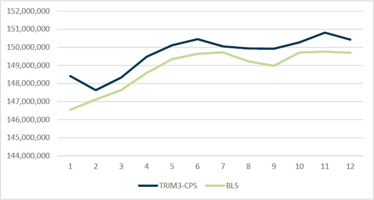
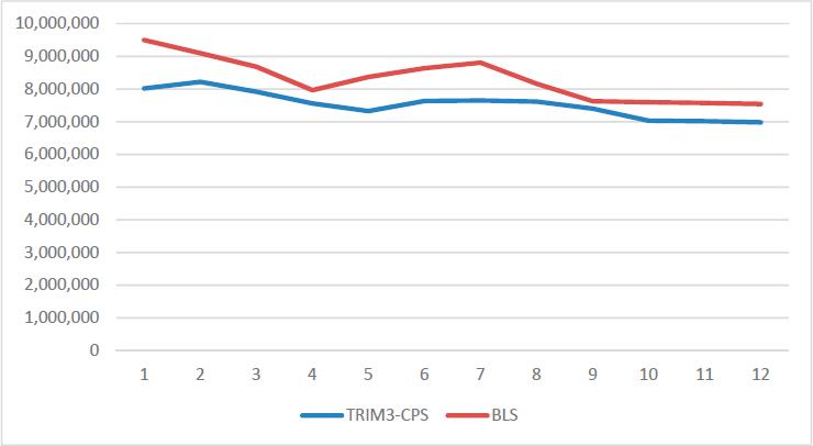
Different methods are used to allocate different types of income across the year, with the most detailed approach taken to allocate earnings and other employment-based income. For individuals who are reported to work fewer than 52 weeks, we first choose a starting-point week and then assign the survey-reported weeks of employment from that point forward (“wrapping” from December to January if needed). The starting point is selected in such a way that the trend in weeks of employment across the months of the calendar year follows the trend from the monthly Bureau of Labor Statistics data (Figure F-1). Similarly, for people who are reported to be unemployed (looking for a job) for part of the year but not the entire year, one or more spells of unemployment is identified (Figure F-2). After the weeks of employment have been identified, earnings are generally assigned evenly across those weeks, implicitly assuming that a person’s weekly earnings are unchanged throughout the year. However, for people who report that they worked part time in some weeks and full time in other weeks, the assignment of weekly earnings reflects those differences.1 Monthly earnings amounts are then generated, treating each month as having 4.333 weeks.
___________________
1 If a person reports usually working full time (35 or more hours per week) but also reports some part-time weeks, we assume he or she works 20 hours per week in the part-time weeks. If a person reports usually working part time, but also reports some full-time weeks, we assume he or she works 40 hours per week in the full-time weeks.
The monthly allocation methods for other types of income are as follows:
- Unemployment compensation: The annual survey-reported unemployment compensation (UC) income amount is generally allocated to all or a subset of a person’s weeks of unemployment, subject to the constraints that UC is not allocated over more weeks than the maximum possible weeks of benefits in a person’s state of residence and that the weekly benefit amount that is assigned falls within the range of minimum and maximum weekly benefit amounts in that state. When people report both UC and earnings during the year, we use state-specific UC rules to estimate a worker’s weekly benefit amount, and that information is also used in the assignment.
- Workers’ compensation: Workers’ compensation is generally divided over all weeks in which a person was either unemployed or out of the labor force; but a portion of recipients are simulated to receive their workers’ compensation as a lump sum.
- Child support and alimony: The number of months over which alimony and child support income amounts are allocated is determined probabilistically based on look-up tables generated from the Survey of Income and Program Participation. Different tables are used for families that do and do not receive TANF; within a subgroup, the probability of a particular number of months of positive child support varies by the annual amount of child support or alimony income, in ranges. Once a number of months is established, the specific months are selected randomly.2
- Other unearned income: Other unearned income amounts—including Social Security, pension income, interest, dividends, rental income, veterans’ payments, regular contributions, educational assistance, black lung/miner benefits, and unspecified “other” income—are allocated evenly across the months of the year.
Note that the above discussion of the monthly allocation of annual values does not mention SSI, TANF, or SNAP amounts, each of which is also reported in the CPS-ASEC in annual terms. Monthly amounts for those programs are developed as part of the baseline simulations, described below.
___________________
2 For people who report both child support and TANF income, and whose annual child support income equals their state’s “pass through” amount times their reported months of TANF income, the months of child support receipt is automatically set equal to the months of reported TANF receipt.
Immigrant Status
The CPS-ASEC asks if people are citizens and, if they are not, asks when they came to the United States. However, the survey does not ask about a noncitizen’s legal status—whether she or he is a lawful permanent resident (LPR), refugee/asylee, temporary resident (e.g., residing in the United States with a student or work visa), or unauthorized immigrant. Whether a noncitizen is potentially eligible for various benefits and for some tax credits depends on his/her specific legal status.
To enable detailed modeling of the program rules regarding immigrant eligibility, an immigrant status is assigned to each noncitizen (Table F-1). The methods follow an approach first developed by Dr. Jeffrey Passel and Dr. Rebecca Clark (1998) and further developed by Dr. Passel and coauthors (Passel, VanHook, and Bean, 2006, Passel and Cohn, 2011). In brief, the approach proceeds as follows:
- Reclassification of some naturalized citizens: Among people who report being naturalized citizens, 1.9 million are reclassified as noncitizens, based on prior analyses indicating overreporting of naturalization.
- Temporary residents: 1.4 million noncitizens are identified as temporary residents, due to having demographic and employment characteristics suggesting that they are in the United States on a work or student visa.
- Refugees/asylees: Noncitizens are initially identified as refugees/asylees if, in the year that they entered the United States, more than one-half of the people arriving from their country of origin were refugees or asylees. Some random adjustments are made to the initial determinations as needed to come closer to externally derived targets. The final results include 1.3 million noncitizens imputed to have had an initial status of refugee or asylee.
TABLE F-1 Key Results of Immigrant Status Imputation Procedures, CY 2015 CPS-TRIM Data
| Group | Imputation result |
|---|---|
| Status Modified from Naturalized Citizen to Noncitizen | 1.9 million |
| Total Noncitizens After Adjustment | 24.9 million |
| Imputed to be Temporary Residents | 1.4 million |
| Imputed to be Refugees/Asylees | 1.3 million |
| Imputed to be LPRs | 11.5 million |
| Imputed to be Unauthorized Noncitizens | 10.7 million |
- Among noncitizens not already identified as refugees/asylees or temporary residents, people are identified as LPRs if they are in an occupation that would require legal status (e.g., police officer) or if they report a type of benefit that would require legal status.
- Among the remaining noncitizens, people are probabilistically assigned to either LPR status or unauthorized immigrant status based on their characteristics, coming acceptably close to a set of externally derived targets for the number and characteristics of unauthorized immigrants in the CPS-ASEC data.
- Adjustments are made as needed to the person-level imputations to ensure logical intrafamily consistency.
Dr. Passel develops the targets that guide the imputation of unauthorized status using numerous sources of data on legal entrants to the United States over time and adjusting those figures to account for age progression, naturalization, emigration, and death; this results in estimates of people in the country legally. The total noncitizens in the CPS-ASEC data minus the number in the country legally provides the estimate of unauthorized immigrants in the CPS-ASEC data. The final imputations include 10.7 million unauthorized immigrants and 11.5 million LPRs.
Baseline Simulation Methods
Before any use of TRIM3 to assess the potential impacts of changes in policies, a set of baseline simulations must first be completed. The baseline simulations apply the actual rules that were in place in the year of the data being used as input to the households in those data. The simulations create new items of information for each household, telling if they are eligible for various programs, their level of tax liability, and so on. Each simulation follows the same steps that an individual would use to compute his or her income taxes or that a caseworker would use to determine a family’s eligibility for benefits. Simulations of benefit programs also identify which of the eligible people or families receive benefits from, and hence participate in the program, in order to create a simulated caseload that comes close to the actual caseload size and characteristics obtained from external administrative and government sources.
In the case of most of the benefit programs discussed here (all except CCDF-funded child care subsidies), the simulated data on program receipt are used to augment, and to some extent replace, the survey-reported CPS-ASEC data on those programs. Specifically, the CPS-ASEC includes annual income and benefit amounts for SSI, TANF, SNAP, and LIHEAP, and includes variables telling whether a household is in public or subsidized housing and whether a family receives benefits from WIC. However, this information is
not sufficient to support modeling of alternative policies, for a few reasons. First, the reported amounts and caseloads fall substantially short of targets, even after missing survey responses have been adjusted through the Census Bureau’s imputation procedures. Second, the survey-reported receipt sometimes does not appear consistent with known program rules. For example, there are cases of families with no young children and no woman of childbearing age who report WIC benefits, or people reporting SSI who are younger than 65 and whose other data show no indications of disability. Third, even when individuals report receiving benefits from a given program appear generally eligible for that program, the specific amounts that are reported are usually not perfectly consistent with what would be computed by applying the program rules to the family’s income and demographic data. That is to be expected, since many respondents probably round various dollar amounts, and since some amounts are imputed by the Census Bureau. However, when alternative policies are modeled, the benefits under the new policy are computed based on the rules and the survey-reported household income and demographic data; it is important that the only difference between the baseline benefit amount and the alternative benefit amount is that resulting from the policy change, and the only way for that to be the case is for the baseline benefits to be computed with the same methods that will be used in modeling the alternative policies.
Although the CPS-ASEC includes questions about benefit receipt, the survey does not ask respondents about their tax liabilities. The Census Bureau imputes federal and state income tax liabilities to the households in the CPS-ASEC as part of their development of SPM poverty estimates, and they make those imputations available to researchers; however, to ensure complete consistency with other simulated data, the TRIM3 analyses use the baseline tax liability amounts modeled within the TRIM3 system.
The baseline simulations are performed sequentially, so that information from one baseline can be used as input to subsequent simulations, creating an internally consistent picture of families’ benefits, tax liabilities, and tax credits. Cash benefits are simulated first, followed by in-kind benefits (which may include cash benefits as part of their income definition). Similarly, federal income taxes are simulated prior to state income taxes, since many states’ income tax systems use information from the federal tax form. Additional key points about the baselines are provided below.
Baseline Simulations of Benefit Programs
In general, the simulations of benefit programs proceed in three steps: determining eligibility, computing potential benefits, and determining which eligible families are enrolled in the program. These steps are performed month-by-month, capturing the fact that a family with part-year work
might be eligible for different benefits during months of employment than during months of unemployment.
The steps in eligibility modeling often include: defining the “filing unit” (the individuals in the household who are considered together in assessing eligibility and benefits); applying immigrant-related restrictions and other restrictions based on demographic characteristics (for example, two-parent families are ineligible for TANF in some states); determining countable income; applying assets tests; and applying income tests. When eligibility policies vary by state, TRIM3 captures the state-by-state variations in eligibility policies with a high degree of detail.
Benefits are computed according to each program’s actual policies. Benefit computation formulas often vary by income levels and other characteristics, but may also be flat amounts (for example, in the case of LIHEAP). In the case of housing and child care subsidies, TRIM3 computes the value of the benefit as an assumed full value of what is being provided minus the family’s required payment. As with eligibility modeling, state-level variations in benefits-related policies are captured in detail. Benefit amounts are computed for all families and individuals who appear to be eligible, including those for whom there is a benefit amount in the public-use data. This ensures that all the baseline benefit data are completely consistent with the known policies and the reported income and family characteristics, which is an important precondition for assessing the impact of policy changes.
The specific methods for determining which eligible families or individuals are enrolled in a program vary across the programs, but similar principles are followed. They are:
- If an eligible person or family reported receiving a benefit in the CPS-ASEC survey (a true report, not an imputed report), that person or family is automatically included in the program’s caseload.
- Among eligible people/families who did not report receipt of a benefit, recipients are selected probabilistically in a way that comes acceptably close to the size and characteristics of the actual caseload—the caseload “targets.” Those targets are derived from administrative data, with adjustments as needed for greater consistency with the TRIM3 universe. (For example, targets for SSI exclude the institutionalized recipients, since the CPS-ASEC surveys only noninstitutionalized households.)
- Probabilistic assignments are made by comparing a potential assistance unit’s estimated probability of enrollment (based on a variety of characteristics, which vary across programs) to a random number. Specifically, if the unit’s probability of participation exceeds the unit’s random number for purposes of participation for this program, the unit is simulated to participate.
- For each benefit program, a unique set of random numbers is used for all probabilistic enrollment assignments for that program for a particular year of data. This ensures that when an alternative simulation results in a change to the unit’s probability of participation, any changes in enrollment decisions are logically consistent with the alternative policy change. For example, assume that a hypothetical policy change increases a unit’s potential TANF benefit, raising the unit’s probability of participation. If the unit participated in TANF in the baseline, the unit will not stop participating; if the probability was previously higher than the random number, the now-higher probability will still be higher than the random number, since the random number did not change. However, if the unit was previously an eligible nonparticipant, the unit may start to participate, if the now-higher probability exceeds the unchanged random number.
- Only families and individuals who are simulated to be eligible for a program are considered as possible program recipients. Because of that assumption, if an ineligible person or family reports a benefit, we implicitly assume that the report was made in error, and that person or family is not included in the simulated caseload. This simplification avoids complications that would arise from applying policy changes to a simulated baseline caseload that included ineligible participants.3
Details of the methods for each simulation are available on the TRIM3 project’s website (http://trim3.urban.org). Here, we summarize key points and note some challenges involved in modeling each program.
- SSI:
- Portion of program modeled: Benefits to individuals in households (not institutionalized).
- Timeframe: Monthly
- Policies: Primarily national-level; state-level supplement amounts are obtained from a combination of national and state-level sources.
___________________
3 Future model development could consider some allowance for technically ineligible units being in the caseload, based on administrative estimates of the extent of that type of enrollment error. However, this would require decisions regarding how to handle these cases in alternative simulations. (For example, if an ineligible unit that has been included in the caseload is modeled to receive higher earnings due to a minimum wage increase, it is unclear whether it would be more appropriate to continue to include the unit in the caseload, or whether to assume the unit would lose benefits due to exceeding the eligibility limit by an even greater amount.)
-
- Eligibility and benefits challenges: Assessing potential eligibility based on age (65 or older) is straightforward, but assessing potential eligibility based on disability is complex. For adults, disability is inferred through a combination of the survey-reported reason for not working and survey-reported disability income. Disability cannot be assessed for children.
- Caseload selection: For adults, the caseload is aligned to targets by reason for eligibility (age vs. disability), type of unit (single or couple), state, and citizenship status. For children, after identifying children whose parents report them as SSI recipients, the rest of the caseload is randomly selected from among children in income-eligible families, to reach targets by family structure (two-parent, single-parent, no-parent) and by state. We also come close to the number of children in multiple-recipient households (about 500,000), according to analysis by the Government Accountability Office (Government Accountability Office, 2016).
- TANF:
- Portion of program modeled: TRIM3 models cash aid provided through TANF and Separate State Program (SSP) funds. The model also identifies benefits paid through Solely State Funded (SSF) programs; those are separately classified as SSF, not TANF.
- Timeframe: Monthly
- Policies: Almost entirely state-level; source of rules is the Welfare Rules Database (for the 2015 policies, see Cohen et al., 2016).
- Eligibility and benefits challenges: The data do not allow us to directly assess if a family that appears eligible may in fact be ineligible due to previously having reached a time limit. A portion of otherwise-eligible families are treated as ineligible due to time limits, in order to reach estimated state-level targets for time-limited families; the targets are derived from administrative data. Also, the families simulated to be eligible nonparticipants include some who have been excluded due to failure to meet program requirements. Benefits are computed based on family characteristics and detailed state policies, but they do not incorporate the impact of either special-needs payments (additional payments in some states for reasons such as the start of the school year, pregnancy, or a special hardship) or monetary sanctions (reductions of benefits for failure to comply with a requirement).
- Caseload selection: For the TANF/SSP caseload, key targets include type of unit (single-parent units with and without
-
- earnings, two-parent units, and child-only units by various reasons for child-only status), state, and presence of noncitizens. An underlying participation function also incorporates varying probabilities of participation by other characteristics, including level of potential benefit, race/ethnicity, and number and ages of children. There is no single source for SSF targets; SSF targets are derived from caseload-reduction reports submitted to the federal government and from various state data systems and reports.
- CCDF:
- Portion of program modeled: Children subsidized through CCDF funds. (States may combine other funds with CCDF funds to serve more children; however, the baselines for this analysis identify only the children viewed by Health and Human Services’ Administration for Children and Families as served by CCDF funds.)
- Timeframe: Monthly
- Policies: Almost entirely state-level; source of rules is the CCDF Policies Database (for 2015 policies, see Stevens et al., 2016).
- Eligibility and benefits challenges: In some cases, the family’s required copayment depends in part on the hours that the children require care; that is inferred based on the mother’s usual hours of work. The model treats all months of the year the same, without any special treatment of the summer months.
- Caseload selection: The key target is the average monthly number of children served, by state. Probabilities vary by age of child, single-parent vs. two-parent families, and relative income levels. The simulation also takes into account the survey-reported amount of child care expenses; to the extent feasible, eligible families whose simulated copayment is similar to what they reported spending in child care expense have a higher likelihood of being included in the simulated caseload, and eligible families whose simulated copayment is quite different from what they reported spending (e.g., we simulate that their copayment would be $50/month, but they reported spending $3,600 across the year) have a lower likelihood of being included in the simulated caseload.
- Public and subsidized housing:
- Portion of program modeled: Public housing and vouchers for obtaining rental housing.
- Timeframe: Monthly
- Policies: The same policies are applied nationally for the definition of income and the computation of each assisted
-
- household’s required rent. Fair Market Rents (FMRs) are obtained from the U.S. Department of Housing and Urban Development (HUD), and vary by county and metropolitan area.
- Eligibility and benefits challenges: Because eligibility policies may vary from one Public Housing Authority to another, baseline simulations do not explicitly model eligibility beyond requiring that household income be below 80 percent of area median income. However, among households reported to be in public or subsidized housing in the CPS-ASEC data, required rents are estimated based on the national-level formulas and the household’s income, and each assisted household’s subsidy value is estimated as the appropriate FMR (based on the county or metropolitan area and the needed apartment size) minus the required rent.
- Caseload selection: Unlike other simulated benefit programs, the public and subsidized housing simulation does not include a participation function or alignment to external targets. Among households reported to be in public or subsidized housing in the CPS-ASEC data, if the required rent is less than the assumed FMR (based on location and estimated number of bedrooms), the household is treated as enrolled. If the required rent is greater than the assumed FMR, the household is treated as though it is not in public or subsidized housing.
- SNAP:
- Portion of program modeled: All recipients except those who are homeless or in institutions.
- Timeframe: Monthly
- Policies: Policies are obtained from the Food and Nutrition Service (FNS); some state-level variations are obtained from the SNAP State Options Report (Food and Nutrition Service, 2016) and other sources.
- Eligibility and benefits challenges: Estimates of SNAP eligibility are very sensitive to assumptions about which members of complex households would jointly file for SNAP. The TRIM3 methods follow the explicit rules about which family members are required to file for SNAP together and make assumptions about other situations.
- Caseload selection: The key enrollment targets include family structure, presence of cash benefits (SSI or TANF), level of potential SNAP benefit, presence of earnings, state, and citizenship status.
-
WIC:
- Portion of program modeled: Benefits to infants, their mothers, and young children. (Benefits to pregnant women are captured only to the extent that a childless woman of childbearing age reports WIC in the CPS-ASEC.)
- Timeframe: Monthly
- Policies: Policies are obtained from FNS data. Basic policies are national, but there is state variation in the value of the benefit and in the certification period for children.
- Eligibility and benefits challenges: The WIC program does not explicitly define whose income is counted in determining eligibility; we assume that the eligibility process considers all people related to the children, including both parents in the case of unmarried couples.4 One aspect of WIC eligibility—nutritional risk—cannot be observed in the CPS data. The simulation assumes that all people who pass the demographic and financial eligibility tests are at nutritional risk.
- Caseload selection: For infants and children, enrollment is aligned to state-level targets.
- LIHEAP:
- Portion of program modeled: Heating and cooling help (weatherization help is not modeled).
- Timeframe: Annual
- Policies: State-specific eligibility policies are obtained from the LIHEAP Clearinghouse website (https://liheapch.acf.hhs.gov). Because most LIHEAP benefits are provided in the winter, based on eligibility determination in the fall, the simulation uses the eligibility policies in place in the fall of the calendar year; specifically, the CY 2015 LIHEAP eligibility simulation used the FY 2016 eligibility policies (which went into effect in October 2015).
- Eligibility and benefits challenges: Local programs may differ in their income definitions or the period over which they assess income, at the point that a household applies for help; we assume all places use annual income.
- Caseload selection: The simulated caseload is aligned to state-specific targets, which are estimates of the unduplicated count of households receiving heating and/or cooling help over that calendar year.
___________________
4 The WIC eligibility estimates produced for the Food and Nutrition Service (Trippe et al., 2018) also use a broad definition of the economic unit. If eligibility was estimated with a narrower unit—considering related subfamilies as separate units—more children would be identified as eligible.
Baseline Simulations of Tax Programs
The simulations of taxes require the identification of the tax unit and then the computation of the tax amounts. People are assumed to pay all the taxes that they owe, and with only a few exceptions they are assumed to take all available tax credits; therefore, the modeling of taxes does not involve alignment to caseload targets in the same way as the modeling of benefits does. However, modeling of income taxes does require additional imputations to estimate items of information not available in the CPS-ASEC data. Key aspects of the tax simulations are:
- Payroll taxes:
- Portion of program modeled: Old age, survivors, disability, and health insurance taxes (OASDHI); includes taxes on self-employment earnings and Civil Service Retirement Service (CSRS) contributions.
- Timeframe: Annual
- Policies: Social Security website
- Federal income taxes:
- Portion of program modeled: Most aspects of individual income tax computation. Some tax features that are applicable only to very high-income taxpayers or very rare situations are not modeled.
- Timeframe: Annual
- Policies: 1040 (and supporting schedule) forms and instructions
- Imputations preceding the modeling: Data from the Internal Revenue Service (IRS) Statistics of Income Public Use File are used to impute amounts of itemized deductions, capital gains/losses, and individual retirement account (IRA) contributions.
- Alignment of usage of selected credits: In general, taxpayers are assumed to take all credits for which they appear eligible. However, the modeling of the child and dependent care expense credit assumes that a portion of the units who appear eligible—based on having working parents, children under age 13, and child care expenses—do not in fact take the credit for some reason (for example, because they are ineligible due to their flexible-spending-account benefits). The take-up of the credit is aligned to data on the actual number of tax units taking the credit.
- State income taxes:
- Portion of program modeled: Most aspects of states’ individual income tax computation. Some tax features that are applicable only to very high-income taxpayers or very rare situations are not modeled.
-
- Timeframe: Annual
- Policies: State-by-state tax rules compiled by a team led by Dr. Jon Bakija, Williams College
2015 Baseline Simulation Results vs. Targets
The 2015 simulations of benefit programs were, in almost all cases, very successful at meeting administrative targets. As discussed above, these simulations generally select a simulated caseload from among the households that appear to be eligible in order to meet overall caseload targets (shown in Table F-2) as well as subgroup targets. The simulation of taxes differs from the simulation of benefits in that there is almost no alignment involved. Instead, the results are determined almost entirely by applying the tax rules to the survey data. Results are then compared to administrative data for validation purposes, but overall results are not aligned to come closer to those targets. The result of the TRIM3 baseline simulations is a data file that comes as close as feasible to capturing the real-world incidence and amounts of benefits and taxes in 2015 (Table F-3).
Benefit Program Simulations Compared with Targets
For SSI, TANF, LIHEAP, and CCDF-funded child care subsidies, the simulated caseloads and aggregate benefits all come very close to administrative data figures. For each of these programs, the simulated caseload and the simulated aggregate benefits are no more than 3 percent from total national targets. In addition, the simulations come very close to the actual distribution of the caseload in terms of state of residence and key demographic characteristics. The aggregate amounts of simulated benefits exceed the amounts according to the survey data (including both truly reported amounts and amounts imputed by the Census Bureau) by 11 percent in the case of SSI, 69 percent in the case of TANF, and 56 percent in the case of LIHEAP. (CCDF-funded child care subsidies are not reported in the survey.)
In the case of SNAP, the simulated caseload is very close to the actual figure, but simulated aggregate benefits fall short of the amount, according to administrative data, by 8.5 percent. This pattern of falling short of target for aggregate benefits while hitting the target for the simulated caseload is consistent with other baseline years. TRIM3 finds fewer units eligible for high benefits than are observed in administrative data, and it makes up for the shortfall by exceeding the target for units eligible for lower benefits. The shortfall in high-benefit units is not unique to TRIM3 and is also observed in eligibility estimates produced by Mathematica Policy Research for the FNS. Despite the shortfall in dollars relative to the administrative data, the simulated aggregate SNAP benefit amount of $63.0 billion is much closer
TABLE F-2 TRIM3-Simulated Benefit and Tax Data versus Targets, 2015
| Counts of Persons or Units are in Thousands; Dollar Amounts are in Millions | CPS-ASEC Reported Dataa | TRIM-Simulated | 2015 Admin. Datab | TRIM as % of Admin. Data |
|---|---|---|---|---|
| SSI (Noninstitutionalized)c | ||||
| Adults with SSI During Year for Self or Child | 6,414 | — | — | — |
| Avg. Monthly Adult Recipients (Persons) | — | 7,103 | 6,958 | 102.1% |
| Avg. Monthly Child Recipients | — | 1,234 | 1,254 | 98.5% |
| Annual Benefitsd | $50,715 | $56,399 | $55,569 | 101.5% |
| TANFe | ||||
| Avg. Monthly Caseload (Families)f | 800 | 1,325 | 1,326 | 99.9% |
| Annual Benefits | $3,931 | $6,646 | $6,462 | 102.8% |
| SNAPg | ||||
| Avg. Monthly Units (Households)f | 12,245 | 22,367 | 22,404 | 99.8% |
| Annual Benefits | $36,602 | $63,039 | $68,859 | 91.5% |
| Public and Subsidized Housing | ||||
| Ever-subsidized Householdsh | 5,760 | 5,165 | 4,635 | 111.4% |
| Annual Value of Subsidy | na | $36,955 | na | — |
| LIHEAPi | ||||
| Assisted Households | 4,205 | 6,747 | 6,748 | 100.0% |
| Annual Benefits | $1,717 | $2,673 | 2,675 | 100.0% |
| WIC | ||||
| Families With Any Benefits | 3,780 | 4,071 | na | — |
| Avg. Monthly Recipients, Infants/Children | na | 5,861 | 5,891 | 99.5% |
| Avg. Monthly Recipients, Womenj | na | 907 | 1,865 | 48.6% |
| Annual Value of Benefit, Pre-rebatek | na | $4,875 | na | — |
| CCDF-funded Child Care Subsidies | ||||
| Avg. Monthly Families with CCDF Subsidy | na | 834 | 840 | 99.4% |
| Avg. Monthly Children with CCDF Subsidy | na | 1,351 | 1,387 | 97.4% |
| Aggregate Value of Subsidy | na | $6,611 | $6,585 | 100.4% |
| Counts of Persons or Units are in Thousands; Dollar Amounts are in Millions | CPS-ASEC Reported Dataa | TRIM-Simulated | 2015 Admin. Datab | TRIM as % of Admin. Data |
|---|---|---|---|---|
| Payroll tax | ||||
| Workers Subject to OASDI Tax | na | 157,185 | 168,899 | 93.1% |
| Taxable Earnings for OASDI | na | $6,748,090 | $6,395,360 | 105.5% |
| Taxes Paid by Workers (OASDI + HI) | na | $560,877 | $541,055 | 103.7% |
| Federal Income Taxes | ||||
| Number of Positive Tax Returns | na | 104,461 | 99,022 | 105.5% |
| Total Tax Liability, Positive Tax Returns | na | $1,312,511 | 1,435,849 | 91.4% |
| Earned Income Tax Credit | ||||
| Returns with Credit | na | 19,712 | 28,082 | 70.2% |
| Total Credit | na | $41,770 | $68,525 | 61.0% |
| State Income Taxes | ||||
| Number of Positive Tax Returns | na | 89,970 | na | — |
| Taxes Paid, Net of Creditsl | na | $318,089 | $340,468 | 93.4% |
NOTE: na = not available; avg. = average; admin. = administrative.
a CPS-ASEC reported data included the data that are “allocated” by the Census Bureau in cases of nonresponse. Items not asked in the survey that are imputed by the Census Bureau (such as tax liabilities) are not shown.
b Administrative figures are adjusted or combined for consistency with simulation concepts. In particular, fiscal year administrative data are adjusted for greater comparability with calendar year simulated data, and benefits paid to individuals in the territories are excluded. Benefits include both federally-funded and state-funded amounts.
c SSI figures include state supplements.
d Administrative data for SSI include retroactive payments, which are approximately 9 percent of total payments; TRIM does not simulate retroactive payments.
e Includes benefits funded by federal TANF money and separate state programs, but not solely state-funded programs. The administrative figure for aggregate benefits is computed as the average per unit benefit from administrative microdata applied to the actual caseload.
f For TANF and SNAP, an average monthly caseload is computed using the CPS-reported number of months that benefits are received.
g The administrative figures for SNAP exclude SNAP disaster assistance.
h Administrative figure is the number of occupied public and assisted units.
i An exact unduplicated number of assisted households is not available; an unduplicated count is estimated using estimates of the overlap between groups receiving heating, cooling, and crisis benefits.
j Benefits to pregnant women are not captured in the TRIM simulation.
k The TRIM benefit amount includes the pre-rebate value of infant formula. An administrative figure for WIC food costs net of the rebate was not available.
l The actual state income tax amount is from the Census Bureau’s Annual Survey of State Government Tax Collections, which reflects tax collections during a fiscal year; TRIM3’s figures are estimates of tax liability during the tax year.
TABLE F-3 TRIM3 Benefits and Expenses Incorporated into the 2015 SPM
| SPM Benefit or Expense | Notes |
|---|---|
| SSI | TRIM3 SSI amounts are used instead of the reported amounts. |
| TANF | TRIM3 TANF amounts are used instead of the reported amounts. |
| SNAP | TRIM3 SNAP amounts are used instead of the reported amounts. |
| WIC | TRIM3 simulated amounts are used instead of the Census Bureau values assigned to people who report WIC receipt in the CPS ASEC. |
| LIHEAP | TRIM3 simulated amounts are used instead of reported amounts. |
| Public and Subsidized Housing | Uses TRIM3 public and subsidized housing subsidies rather than amounts imputed by the Census Bureau to households reporting receipt of public and subsidized housing assistance. TRIM3 follows the Census Bureau SPM methodology of capping the amount of the subsidy counted for the SPM at the share of the SPM threshold representing shelter and utility expenses, less the household’s required rental payment. |
| Child Care Expenses | Primarily reflects CPS reported amount. However, for families simulated by TRIM3 to receive CCDF child care subsidies, reflects the required copayment amount. Child care expenses are counted as an expense in the SPM. |
| Payroll Taxes | TRIM3 simulated amounts are used instead of Census Bureau simulated amounts. |
| Realized Capital Gains/Loss | Statistically matched from the IRS Public Use File as part of the federal income tax baseline. The Census Bureau tax model does not impute capital gains and so they are not included in the Census Bureau SPM. However, capital gains are included in the TRIM3 SPM because they are included in the calculation of TRIM3 federal and state income taxes.a |
| Federal Income Tax | TRIM3 simulated amounts are used instead of Census Bureau simulated amounts. Includes taxes on capital gains (not included in the Census Bureau estimate). Includes refundable credits (EITC and Additional Child Tax Credit). |
| State Income Tax | TRIM3 baseline simulated amounts are used instead of Census Bureau simulated amounts. Includes taxes on capital gains. Includes refundable credits. Replaces Census Bureau simulated amounts. |
a Capital gains are obtained through a statistical match with the IRS Public Use File as part of the TRIM3 federal income tax baseline.
to the actual figure ($68.9 billion) than the amount captured in the survey data ($36.6 billion).
In the case of public and subsidized housing, TRIM3 includes any households living in public or subsidized housing according to the public-use survey data as long as their income is below 80 percent of the area median income published by HUD and their required rent payment would be lower than the HUD Fair Market Rent based on the number of bedrooms estimated for the household and their county or metropolitan area; these methods overshoot by about 11 percent the number of households in public housing or with housing vouchers for low-income families funded by HUD, probably because some of the identified households are receiving other types of housing help.
The WIC simulation comes very close to targets for the number of infants and children with WIC. However, the simulation is only able to capture WIC receipt by women who are the mothers of infants; benefits received by pregnant women are not fully captured because the CPS does not identify pregnancy.
Tax Simulations Compared with Targets
In simulating payroll taxes, the number of workers observed as subject to OASDI taxes is about 7 percent short of the actual figure. However, the aggregate taxable earnings seen in the data and the resulting simulated payroll taxes are somewhat higher than the administrative data target. This pattern of falling short of the target for the number of workers who are subject to OASDI taxes while exceeding the total amount of taxes is consistent with other baseline years and is driven by reported employment and earnings in the CPS-ASEC. A contributing factor to the excess in OASDI taxes is that CPS-ASEC respondents are likely to report their full earnings, rather than their earnings less nontaxable components such as pretax health insurance premium payments and contributions to medical and dependent care flexible benefits plans. Such reductions to earnings are not captured in the baseline simulation.
The federal income tax simulation counts a number of tax returns with positive income tax liability that is 5.5 percent higher than the actual number of returns for tax year 2015, but the model falls short of the actual amount of tax liability on positive-tax returns by 8.6 percent. The shortfall in taxes is likely due to the CPS-ASEC not capturing all the income in the highest portion of the income distribution. The same issue is observed in the simulation of state income taxes, which identifies an aggregate amount of state income liability that is 6.6 percent below the aggregate target.
The simulation also falls short in the identification of units with the EITC. The shortfall in simulated EITC is not unique to TRIM3 and is commonly observed in other microsimulation estimates based on CPS-ASEC
data. Some of the shortfall is explained by the fact that TRIM3 does not model noncompliance with EITC rules. CPS-ASEC data issues may also contribute to the shortfall (Wheaton and Stevens, 2016). TRIM3 assigns EITC to all units found eligible according to the CPS-ASEC data. Assigning additional units to receive the EITC would require modeling noncompliant receipt of the EITC or adjusting the earnings and family composition data in the CPS-ASEC, both of which are beyond the scope of this study.
To validate the TRIM3 SPM calculations, we first calculate the SPM following the Census Bureau methodology using unadjusted CPS-ASEC variables and Census Bureau imputed variables obtained from the Census Bureau’s SPM research file.5 We then substitute TRIM3 variables for the CPS ASEC and Census Bureau imputed variables and compare the effects of the TRIM3 variables on the estimates.
The estimates presented here are comparable with the Census Bureau’s revised 2015 SPM estimates that are included in the Census Bureau’s 2016 SPM report (Fox, 2017). In preparing the 2016 SPM, the Census Bureau revised the EITC, housing subsidy, and work-related expense imputations. For consistency, the Census Bureau re-issued estimates for 2015, using the same methodology, and included the results in the 2016 SPM report. We use the revised 2015 variables for our estimates.
When we use the TRIM3 model to calculate SPM poverty using only the CPS-ASEC and the Census Bureau imputed values, we find that 12.038 million children were in SPM poverty in 2015, compared with 12.026 million according to the Census Bureau (Table F-4).6 Small differences such as this arise because our calculated results are generated using public-use data rather than internal Census Bureau files and because certain household heads younger than 18 who are living with parents are classified as “children” when calculating the SPM threshold in our calculated results, but not in the published results.7
___________________
5 See Fox (2017) for discussion of the Census Bureau’s methods. The SPM research file is available at the Census Bureau’s website at: https://www.census.gov/data/datasets/2015/demo/supplemental-poverty-measure/spm.html.
6 See appendix table A-1 of Fox (2017).
7 The change in the number of children results from TRIM3’s restructuring of “inverted households” in the TRIM3 conversion process. These households are ones in which a teen or young adult is reported to be the household reference person, despite having one or both parents present. Many of these households involve immigrants, and it is likely that the teen or young adult was selected as the reference person because of his/her English capability. TRIM3 reorganizes the inverted households, so that a parent is the household reference person. If the teen is under the age of 18, reclassifying the teen from “head” to “child” increases the number of children in the unit, thus affecting the SPM poverty threshold. If the teen is working, then reclassification as a “child” also affects the unit’s work expenses, as the SPM methodology does not assign work expenses to children under the age of 18 unless they are the head or spouse of the SPM unit.
TABLE F-4 Effect of TRIM3 Adjustments on SPM Child Poverty and Deep Poverty Estimates, 2015
| Children in Poverty | Children in Deep Poverty | |||
|---|---|---|---|---|
| Total (1,000s) | Percent | Total (1,000s) | Percent | |
| Census Bureau (Published) | 12,026 | 16.2% | 3,628 | 4.9% |
| Census Bureau (Calculated) | 12,038 | 16.3% | 3,636 | 4.9% |
| TRIM3 Adjustments: | ||||
| Correction for Underreportinga | ||||
| SSI | 11,462 | 15.5% | 3,388 | 4.6% |
| + TANF | 11,205 | 15.1% | 3,138 | 4.2% |
| + SNAP | 9,502 | 12.8% | 2,081 | 2.8% |
| + WIC | 9,362 | 12.6% | 2,081 | 2.8% |
| + LIHEAP | 9,324 | 12.6% | 2,076 | 2.8% |
| Other TRIM3 Adjustmentsb | ||||
| + Housing | 9,295 | 12.5% | 2,078 | 2.8% |
| + Child Care Expenses | 9,378 | 12.7% | 2,106 | 2.8% |
| + Taxes and Tax Credits | 9,633 | 13.0% | 2,136 | 2.9% |
a The “correction for underreporting” rows show the effects of replacing the CPS ASEC amounts with TRIM3-simulated variables that correct for underreporting. First, TRIM3-simulated SSI is substituted for reported SSI. Starting from that simulation, TRIM3-simulated TANF is then substituted for reported TANF, and so-on. TRIM3 child support income adjustments are incorporated at the same time as TANF.
b The “other TRIM3 adjustments” rows show the effects of replacing the CPS ASEC amounts (obtained from the Census Bureau’s SPM research file) with TRIM3-simulated variables. Starting from the correction for underreporting simulation that includes LIHEAP, TRIM3-simulated housing subsidies are substituted for the Census Bureau imputed subsidies. Next, TRIM3 child care expenses are substituted for the Census Bureau amounts. Finally, TRIM3 payroll taxes, federal income taxes and credits, and state income taxes and credits are substituted for the Census Bureau values. TRIM3 imputed realized capital gains (and loss) are incorporated at the same time as taxes.
SOURCES: Published Census Bureau estimates are from Fox (2017), Appendix Table A-1. Other estimates are obtained from TRIM3 tabulations of the 2016 CPS ASEC.
We next show the incremental effects of substituting TRIM3 variables for the CPS-ASEC and Census Bureau variables in the poverty calculation, focusing first on TRIM3 correction for underreporting of SSI, TANF, SNAP, WIC, and LIHEAP, and then describing the effects of incorporating other TRIM3 variables. We find that substituting TRIM3-simulated SSI income into the Census Bureau SPM poverty definition lowers the estimated SPM child poverty rate from 16.3 percent to 15.5 percent. If we keep the TRIM3-simulated SSI in the SPM definition and next substitute TRIM3-simulated TANF for the CPS-reported amount, the child poverty rate drops from 15.5 percent to 15.1 percent. Replacing CPS-reported SNAP with TRIM3-simulated SNAP decreases the estimated child poverty rate from 15.1 percent to 12.8 percent. Replacing the Census Bureau’s
WIC value with TRIM3-simulated WIC decreases the child poverty estimate slightly—from 12.8 percent to 12.6. Replacing reported LIHEAP with TRIM3-simulated LIHEAP has little effect on the estimated number of children in poverty. Taken together, the TRIM3 adjustments for underreporting reduce the estimated SPM child poverty rate from 16.3 percent to 12.6 percent.
The remaining rows in Table F-4 show the effects on the SPM poverty estimate as other TRIM3 adjustments (housing subsidies, child care expenses, and taxes) are incorporated into the SPM definition. As noted previously, these adjustments do not replace reported variables but instead replace values imputed by the Census Bureau. They are typically included in TRIM3 poverty estimates and analyses to preserve internal consistency between simulated programs and between baseline and alternative policy scenarios.
Incorporating TRIM3 housing subsidies into the SPM estimate that includes TRIM3 correction for underreporting reduces the estimated child poverty rate by 0.1 percentage points. Incorporating TRIM3 child care expenses into the SPM increases the estimated child poverty rate by 0.2 percentage points.8 Substituting TRIM3 taxes and tax credits for the Census Bureau amounts and incorporating TRIM3-imputed realized capital gains and losses increases the child poverty rate 0.3 percentage points.9 Taken together, the TRIM3 corrections for underreporting and other TRIM3 adjustments reduce the child poverty rate from 16.3 percent to 13.0 percent.
The TRIM3 adjustments also affect the deep poverty rate—the share of children below one-half of the poverty threshold. Correction for underreporting reduces the estimated deep poverty rate from 4.9 percent to 2.8 percent for children. Incorporating TRIM3 housing subsidies, child care expenses, and taxes and tax credits has little effect on the deep poverty rate, increasing it by 0.1 percent.
Note that although TRIM3 adjusts for the underreporting of several key elements of family resources, other elements of resources—which may
___________________
8 The TRIM3 SPM estimate allows higher expenses for some families because it does not cap child care expenses (combined with other work-related expenses) at the earnings of the lower earning spouse or partner. As noted previously, TRIM3 does restrict the expenses to parents/guardians who work or are in school. In some cases, the simulated child care copayment may be higher than the reported CPS amount.
9 One reason that the poverty rate increases when the Census Bureau’s tax amounts are replaced with TRIM3-simulated amounts is that the Census Bureau EITC assignment does not prevent unauthorized immigrants from receiving the EITC. Under federal income tax rules, the tax unit head, spouse, and qualifying child must each have a valid Social Security number to claim the EITC. In the absence of this restriction, the TRIM3 SPM child poverty rate would have been 12.3 percent in 2015 (not shown). Thus, if TRIM3 did not deny the EITC to unauthorized immigrants, substituting TRIM3-simulated taxes and tax credits for Census Bureau amounts would have lowered, rather than raised, the SPM child poverty rate.
also be underreported—are used as they appear in the public-use survey data. Rothbaum (2015) compares CPS-ASEC income amounts to aggregates from the National Income and Product Accounts and finds that the CPS-ASEC data for 2012 captured only 72 percent of interest income, 66 percent of unemployment compensation, 60 percent of self-employment income, 28 percent of workers’ compensation income, and 68 percent of total pension income, among other findings. Some poor children are affected by these income amounts. For example, in the CY 2015 CPS-ASEC data used for this analysis, 12 percent of children in SPM poverty (according to our baseline measure) lived in an SPM unit with some self-employment income, and 2 percent lived in a unit with some type of pension income. (These figures include both truly reported amounts and amounts imputed by the Census Bureau when responses are not provided.) To the extent that income amounts that are not adjusted by TRIM3 are underreported by families with children, our estimates of children’s poverty could be overstated.
On the other hand, some of the data imputations made by the Census Bureau could be leading us to identify as nonpoor some children who might be poor. For example, while only 8 percent of poor children live in SPM families that truly reported interest or dividend income (compared with 27 percent of all children), the Census Bureau’s procedures to “allocate” (fill in) missing data increase that percentage to 24 (compared to 62 percent for all children). Regarding the most common type of income—earnings—research by Bollinger and colleagues (forthcoming) finds that when the Census Bureau imputes amounts of earnings due to nonresponse, the imputed figures are biased upward for low earners (and downward for very high earners). If Census Bureau data imputations are assigning too much income of certain types to low-income families with children, that would operate in the direction of understating child poverty.
Critique of TRIM3 Poverty Estimates
Two recent studies have examined the effect on poverty of TRIM3 SNAP adjustments relative to poverty estimates based on survey data combined with linked SNAP administrative case-level data (Mittag, 2016; Stevens, Fox, and Heggeness, 2018). The studies conclude that TRIM3 overassigns benefits to low-income households, thus underestimating the poverty rate.
This finding contradicts our own distributional comparisons, which find that TRIM3 underassigns benefits to the lowest income households. In 2015 we find that 8 percent of TRIM3 SNAP participating units with children had $0 in monthly gross income, compared with 13 percent according
to the SNAP Quality Control Data (QC).10 Twenty-two percent of participating units with children had monthly gross income above $2,000, compared with 12 percent according to the QC. TRIM3’s underassignment of SNAP to the lowest income households stems from an apparent shortfall of such households in the survey data.
A possible explanation for these apparently contradictory results is that the linked data analyses take the survey income data as “truth” when examining the distribution of SNAP households by income level. However, survey income may be misreported or imputed by the Census Bureau for nonresponse. In addition, household composition at the time of the survey may not be the same as household composition at the time benefits are received. These factors may distort the true relationship of income and SNAP benefits when benefits obtained from linked administrative data are compared with survey income.
In contrast, TRIM3 assigns SNAP benefits that are consistent with the income and household composition in the survey data, whether these data are accurately or inaccurately reported or imputed by the Census Bureau for nonresponse. Assigning baseline benefits consistently with the income and household composition in the survey data enables alternative simulations that modify program rule parameters to generate internally consistent results. Such consistency is critical for the types of analyses performed in this report.
While analysis of linked administrative data offers opportunities for insights to improve microsimulation, further research is needed before final conclusions can be reached as to the over- or underestimation of poverty in TRIM3.
POLICY CHANGES TO REDUCE CHILD POVERTY
Under this project, alternative policies were modeled in 11 different policy areas: the Earned Income Tax Credit (EITC), child care expenses, the minimum wage, an employment program, SNAP, housing subsidies, SSI, child allowances, child support assurance, immigrant eligibility for safety-net benefits, and a basic income guarantee. For each policy area, two or more variations of the policies were simulated. After each simulation, children’s SPM poverty was computed using the modified data.
The impact of each policy is estimated by comparing the alternative policy’s results—in terms of child SPM poverty as well as program costs and caseloads—to the baseline results. To capture secondary impacts, the full sequence of benefit and tax programs was modeled for each policy. For example, if earnings increase due to a minimum wage change, the family
___________________
10 The SNAP QC estimates are obtained from table A.3 in Gray, Fisher, and Lauffer (2016).
could become eligible for lower TANF and SNAP benefits; could have to pay higher contributions toward subsidized housing or subsidized child care; would owe higher payroll taxes; and would likely see a change in federal or state income tax liability or tax credits.11
This chapter first reviews assumptions used throughout the simulations, regarding program participation, family expenditures, and employment and earnings impacts. We also summarize some strengths and limitations of these approach. The remainder of the chapter then describes, for each policy area, the specific methods and assumptions used to simulate that option—both the explicit policy changes and any assumed changes in employment status or hours of work. Results are also briefly described.
This work builds on prior work by TRIM3 project staff to assess the anti-poverty impacts of policy changes, individually and as a package. See Giannarelli, Morton, and Wheaton (2007) and Lippold (2015) for projects assessing how policy changes could reduce poverty across the entire population and Giannarelli and colleagues (2015) for a prior project examining the potential for policies to reduce child poverty.
OVERVIEW OF SIMULATION ASSUMPTIONS
Assumptions needed to be made about the extent to which the policy changes would change families’ behavior in three areas: program participation, expenditures that impact the SPM, and employment or hours of work. A decision also needed to be made regarding the modeling of benefit programs with fixed budgets.
Program Participation Decisions
Regarding program participation, one type of change happens automatically: If a family becomes ineligible for a program, it stops receiving the benefit. However, assumptions are needed for the treatment of families who become eligible for a different benefit amount due to the policy change or who become newly eligible. We made the simplifying assumption that a family already receiving benefits from a program before the policy change (in the baseline simulation) would continue to participate in the program even if its benefit fell; although in reality a family might decide to stop participating due to a drop in potential benefit, modeling that type
___________________
11 This analysis does not pick up any impacts on a family’s SPM poverty level due to changes in medical out-of-pocket spending. Those expenses could be affected by changes in Medicaid or CHIP eligibility or enrollment, enrollment in employer-sponsored health insurance, or eligibility for or use of health insurance exchanges and associated tax credits. Also, this analysis did not capture changes in eligibility for free or reduced-priced school meals.
of change would complicate the interpretation of the simulation results. In the case when a policy change causes a family to become newly eligible for a program, the model’s internal participation methods were generally used to estimate whether or not that family would begin to receive the benefit. Some specific assumptions regarding the program participation decisions are discussed in the sections on the individual policies.
A change in participation in one program can have secondary impacts on other programs or types of income. For example, because SNAP recipients are eligible for WIC even if their income is higher than the WIC eligibility estimates, a change in SNAP enrollment status can affect a family’s WIC eligibility. Also, because most states’ TANF programs retain all or a portion of the child support paid to TANF recipients, a change in whether a family receives TANF can also change its child support income.
Family Expenditure Decisions
Two key types of expenses affect the program simulations and the SPM poverty calculations and housing and child care expenses. The modeling assumes that changes in a family’s income—for example, higher earnings due to a minimum wage increase—do not result in the family moving to a different apartment or child care provider. Like the assumption of constant program participation behavior, this ensures that simulated changes in a family’s economic well-being are closely tied to the modeled policy change. Of course, for a family with a housing subsidy or child care subsidy, the required rental payment or copayment could change when income changes, and those changes are modeled.
In the case of child care, the one type of behavioral change that may be modeled is the imputation of new child care expenses for some parents who are modeled to start working. When that possibility is modeled, previously estimated equations are used to estimate the probability that a newly working family will need to pay for nonparental care, and if so, the amount of the child care expense. The equations are calibrated so that, when applied to all the families in the CY 2015 CPS-ASEC data, they approximate the incidence and amount of child care expenses reported in the CPS-ASEC data, overall and by income group. The equations predict that the majority of low-income working families do not have any nonparental child care costs, consistent with what is reported in the survey.
Two other categories of expenses that affect the SPM poverty calculation—out-of-pocket medical expenses and child support payments (when a member of the family is paying child support to someone living elsewhere)—are treated as constant across the simulations. The model is not programmed to estimate changes in out-of-pocket health spending due to the types of programmatic or income changes modeled in this project,
and it is not currently able to estimate how income or employment changes could affect a noncustodial parent’s payment of child support.
Employment and Earnings Changes
Changes in whether individuals were employed and in their hours of work were implemented for almost all the simulations, based on specifications provided by the Committee. These types of changes sometimes involved numeric “targets” for people to start working or stop working, based on the Committee’s interpretation of the available econometric evidence. In those cases, the specific people to start or stop working were randomly selected from among those people affected by the policy. In other cases, reductions or increases in hours of work per week were specified for everyone affected by a policy in a certain way. (Details for each policy area are described below.)
Note that the employment and earnings effects were not explicitly restricted to poor families with children. Depending on the specific policy and how the employment and earnings changes were defined and implemented, those changes might have affected nonpoor families, or in some cases might have affected families without children. For example, a minimum wage increase affects low-wage workers even if they live in higher-income families and/or families with children. As another example, EITC employment and earnings changes were restricted to families affected by the EITC changes, meaning that their earnings were low enough to be eligible for the EITC, although only a portion of these individuals are poor. Unless otherwise noted, employment and earnings changes discussed in this Appendix include all of the individuals for whom these changes are modeled, without restriction to poor or low-income families with children.
Changes in employment were assumed to affect unemployment compensation and workers’ compensation in some cases. Specifically, if a person selected to start working had either unemployment compensation or workers’ compensation, that income was assumed to change to $0 due to the new job. In the case of people selected to stop working, unemployment compensation benefits were added only in the case of job loss due to minimum wage increases. In all other simulations with reductions in employment, the job loss was assumed to be voluntary, meaning that no unemployment compensation would be paid.
In all cases, the assumed changes in employment, earnings, and/or other incomes were imposed for the duration of the policy simulation, so that all the simulations of benefit and tax programs for that policy option would consistently treat the person as having the modified employment/earnings/income data. For example, if a person who starts working was previously eligible for safety-net benefits, the levels of potential benefits may decline,
or he or she might become ineligible for some of the benefits. A new worker might be modeled to start to have child care expenses; but might also become eligible for child care subsidies.
Changes in employment status also affect a person’s estimated level of work expenses other than child care. Following the Census Bureau’s SPM methods, a family’s resources are offset by $40.07 for each week that an adult has earnings to reflect spending on transportation and other work expenses (other than child care). For example, if a mother is simulated to move from no work during the year to 52 weeks of work due to one of the policies, the increase to her resources due to the new earnings is offset by $2,084 for purposes of the SPM calculation; conversely, if a mother is simulated to stop working, the reduction to her resources is partially offset by the fact that she is no longer treated as having those work-related expenses. These changes somewhat mitigate the changes in poverty status produced by changes in employment status.
Programs with Fixed Funding
A final issue regarding the simulation assumptions concerns the modeled benefit programs that operate with fixed amounts of funding: LIHEAP, WIC, TANF, and CCDF-funded child care subsidies. The above procedures resulted in some changes to the simulated total benefits costs of these programs as a secondary impact of other policy changes. We did not attempt to recalibrate caseloads or benefits to hold spending constant.
Strengths and Limitations of this Approach
The use of this type of microsimulation modeling allows us to consider the impacts of the potential policies using consistent methods and a consistent metric—the Supplemental Poverty Measure—for all policies. In effect, microsimulation allows us to “try out” the policies using data on a representative sample of the U.S. population. Given the characteristics of the input data and the assumptions described above, the TRIM3 computer code can compute what would happen to a particular family’s economic resources under a proposed policy. The simulations capture not only the direct impacts of policies but also the secondary impacts—for example, the fact that an increase in a child’s SSI benefit could affect the family’s SNAP benefit, since SSI is considered cash income in determining SNAP eligibility and benefits. These calculations are all simulated by the model’s computer code with as much accuracy as possible, given our understanding of the policies and the limitations of the input data.
Of course, there are limitations to these approaches. One overall limitation is the uncertainty in the modeling of behavioral changes, and in
particular in the modeling of employment and earnings changes. As discussed above, this analysis imposed employment and earnings changes specified by the members of the Committee. Another overall limitation is that TRIM3 focuses on the year represented by the input data; it does not currently include the ability to age the population into the future and to capture how the policy changes could affect individuals in successive years, within the broader context of a changing population and economy. Focusing on this particular analysis, other limitations include the fact that the “baseline” data represent 2015, and the fact that mechanisms to pay for the new policies were not modeled.
Because of these issues, it is quite possible that, even if one of the Committee’s policies were put into place exactly as described here, the actual anti-poverty impact could differ from the impact modeled here. However, we do not have a quantitative estimate of the extent of this potential deviation. Looking back at past TRIM3 analyses of the anti-poverty impacts of potential policies, it is almost never the case that a simulated policy is enacted exactly as it was modeled, and without any other policy changes or economic changes occurring at the same time.12
Nevertheless, within the assumptions and population data used for this analysis—in the terminology of economics, “all else equal”—microsimulation modeling provides a way to assess the anti-poverty impacts of the different policies, using the same data, computation mechanisms, and assessment metrics for each one.
EITC
The Committee requested exploratory analysis of several changes to the EITC in the federal income tax system. The two options selected for final analysis were these:
- EITC #1: An expansion of the phase-in range of the EITC, based on a proposal from the Children’s Defense Fund (Children’s Defense Fund, 2015).
- EITC #2: A 40 percent increase in both the credit rate and the phase-out rate.
___________________
12 For example, Zedlewski and colleagues (1996) estimated that the federal welfare reform legislation proposed in early summer of 1996 would increase the number of poor children by 1.1 million. In fact, child poverty declined in the years following welfare reform. However, a major driver of the estimated increase in children’s poverty was the expected loss of food stamps by immigrant children; instead, the year following the passage of the initial legislation, a subsequent bill restored benefits for immigrant children who were living in the United States at the time that the first law was enacted. Also, the late 1990s saw very high levels of GDP growth, which was not foreseen or accounted for by the 1996 modeling.
EITC Policy: Implementation Assumptions
For each policy, we determined the set of EITC parameters consistent with the Committee’s requests (Table EITC-1). For each option, the modified policies replaced the baseline EITC policies in the simulation of federal income taxes, with no other changes made in any other aspect of federal income tax law. For example, the simulations of the alternative EITC policies retain the current-law rule that the taxpayer, spouse (if present), and qualifying children must all have a Social Security number (SSN) to claim the EITC for the qualifying children. (Citizens and legal immigrants are assumed to all have SSNs; unauthorized immigrants and temporary residents do not have SSNs.)
Because many states have state EITC policies that use information from the federal EITC, assumptions were needed regarding those interactions. These simulations assume that there would be no explicit changes in states’ EITC parameters due to the simulated federal changes. Therefore, in a state computing their state EITC as a percentage of a taxpayer’s federal EITC, any increase in the federal EITC will also cause the state EITC to increase.
EITC Policy: Employment and Earnings Effects
Based primarily on econometric analyses conducted by Hoynes and Patel (2017) and Eissa and Hoynes (2004), the Committee specified a set of changes in both employment and hours of work for unmarried and married mothers (Table EITC-2). For unmarried mothers, both EITC policies were assumed to increase employment; for married mothers, the 40 percent EITC increase was assumed to reduce employment and also reduce annual hours of work. (No changes were specified for men’s employment status or hours of work.)
The Committee also requested that the new employment among unmarried mothers be assigned in such a way that the educational distribution of EITC recipients remains approximately the same as in the baseline data, and that the characteristics of new jobs (weeks, hours, and hourly rates) be consistent with the job characteristics of current EITC recipients in each of five educational-attainment groups: less than high school, high school, some college, 2-year college degree, and 4-year college degree or more.
To implement the employment effects, we began by counting the numbers of unmarried and married women who are mothers of a child under age 18 who are not students and who do not have a disability; those counts came to 10.144 million unmarried mothers and 25.107 million married mothers. The targeted numbers of women starting jobs and leaving jobs were obtained by applying the percentage point changes (Table EITC-2) to those universes. For example, in modeling EITC Policy #1 (the expanded
TABLE EITC-1 EITC Parameters for the Two EITC Policy Options
| Credit Rate (Phase-in) | Maximum Earnings to Which Rate Applied | Maximum Credit | Earnings When Phase-out Begins | Phase-out Rate | Earnings When Eligibility Ends | |
|---|---|---|---|---|---|---|
| Actual 2015 EITC Policies | ||||||
| Single, No Children | 7.65% | $6,580 | $503 | $8,240 | 7.65% | $14,820 |
| Single, One Child | 34.00% | $9,880 | $3,359 | $18,110 | 15.98% | $39,131 |
| Single, Two Children | 40.00% | $13,870 | $5,548 | $18,110 | 21.06% | $44,454 |
| Joint, No Children | 7.65% | $6,580 | $503 | $13,760 | 7.65% | $20,340 |
| Joint, One Child | 34.00% | $9,880 | $3,359 | $23,630 | 15.98% | $44,651 |
| Joint, Two Children | 40.00% | $13,870 | $5,548 | $23,630 | 21.06% | $49,974 |
| Single, >= Three Children | 45.00% | $13,870 | $6,242 | $18,110 | 21.06% | $47,747 |
| Joint, >= Three Children | 45.00% | $13,870 | $6,242 | $23,630 | 21.06% | $53,267 |
| EITC Policy #1—Expanded Phase-in Range | ||||||
| Single, No Children | 7.65% | $6,580 | $503 | $8,240 | 7.65% | $14,820 |
| Single, One Child | 68.00% | $6,484 | $4,409 | $11,541 | 15.98% | $39,131 |
| Single, Two Children | 74.00% | $8,875 | $6,567 | $13,269 | 21.06% | $44,454 |
| Joint, No Children | 7.65% | $6,580 | $503 | $13,760 | 7.65% | $20,340 |
| Joint, One Child | 68.00% | $6,484 | $4,409 | $17,061 | 15.98% | $44,652 |
| Joint, Two Children | 74.00% | $8,875 | $6,567 | $18,789 | 21.06% | $49,973 |
| Single, >= Three Children | 79.00% | $10,300 | $8,137 | $15,199 | 25.00% | $47,747 |
| Joint, >= Three Children | 79.00% | $10,300 | $8,137 | $20,640 | 24.94% | $53,267 |
| Credit Rate (Phase-in) | Maximum Earnings to Which Rate Applied | Maximum Credit | Earnings When Phase-out Begins | Phase-out Rate | Earnings When Eligibility Ends | |
|---|---|---|---|---|---|---|
| EITC Policy #2—40% Increase in Phase-in and Phase-out Rates | ||||||
| Single, No Children | 10.71% | $6,580 | $705 | $8,240 | 10.71% | $14,820 |
| Single, One Child | 47.60% | $9,880 | $4,703 | $18,110 | 22.37% | $39,131 |
| Single, Two Children | 56.00% | $13,870 | $7,767 | $18,110 | 29.48% | $44,454 |
| Joint, No Children | 10.71% | $6,580 | $705 | $13,760 | 10.71% | $20,340 |
| Joint, One Child | 47.60% | $9,880 | $4,703 | $23,630 | 22.37% | $44,651 |
| Joint, Two Children | 56.00% | $13,870 | $7,767 | $23,630 | 29.48% | $49,974 |
| Single, >= Three Children | 63.00% | $13,870 | $8,738 | $18,110 | 29.48% | $47,747 |
| Joint, >= Three Children | 63.00% | $13,870 | $8,738 | $23,630 | 29.48% | $53,267 |
TABLE EITC-2 Changes in Mothers’ Employment and Earnings Due to EITC Policy Options
| EITC #1 | EITC #2 | |
|---|---|---|
| Unmarried Mothers (10.144 million a) | ||
| Percentage Point Change in Employment Rate | Pos. 3.0 | Pos. 7.4 |
| Target Number of New Jobs | 304,000 | 771,000 |
| Married Mothers (25.107 million a) | ||
| Percentage Point Change in Employment Rate | — | Neg. 0.8 |
| Target Number Stopping Work | 0.201 mill. | |
| Change in Annual Hours of Work, if Working and Receiving EITC | — | Neg. 100 hours |
a Mothers with at least one child under age 18, who are not students and who do not have a disability.
phase-in range), the Committee selected a 3.0 percentage point increase in the employment rate of unmarried mothers; 3.0 percent of 10.144 million women gives an estimate of 304,000 newly employed unmarried mothers due to the EITC policy.
Before selecting specific women to either start or stop working, preliminary simulations were needed to determine which women would be affected by the EITC changes in ways that might induce labor force changes. Specifically, we do not want to assign a new job to an unmarried mother who, even if she took the job, would be ineligible for the EITC (for example, due to immigrant status, or due to unearned income placing the tax unit above the maximum-allowable adjusted gross income or investment-income limit); and we do not want to simulate a married woman to stop working who, if she stopped working, would no longer be eligible for the EITC (because her husband is not working). To gain this information, we conducted preliminary simulations in which we simulated all employed unmarried mothers to start working, and all employed married mothers to stop working, and observed which tax units were able to take the EITC under each of the new EITC policies. This identifies the potential universes from which the women starting or leaving jobs can be selected; we also looked at the information on potential new workers by education group. A final preparatory task was to tabulate average job characteristics among unmarried mothers modeled as taking the EITC in the baseline data; average weeks, hours, and wages were computed separately for those working full time and full year vs. those working either part time or part year (Table EITC-3).
The final simulations of the EITC policies used the preparatory information described above.
Increased Employment for Unmarried Mothers
For each policy option, a portion of unmarried women who would gain EITC eligibility by starting to work were randomly selected to start working, with the probabilities varying by educational attainment. Specifically, for the universe of women who would be able to take the EITC if they started to work, the probabilities of starting to work across the education groups have the same relationship to each other as the probabilities that an unmarried employed mother currently takes the EITC across the education groups. Table EITC-4 shows the result of this process for EITC Policy #1. For example, among unmarried employed mothers who are not ineligible due to citizenship/immigrant status, the likelihood of taking the EITC is about two times as high for women with exactly a high school education (81%) as it is for those with at least a 4-year degree (40%); likewise, among unmarried mothers who could gain EITC eligibility by starting to work, the probability of taking a job was about twice as high for the high-school
TABLE EITC-3 Among Unmarried Mothers Taking the EITC in 2015, Average, by Educational Attainment: Percentage Working Part Time vs. Full Time, and Mean Weeks, Hours, and Wages for Each Group
| Percent by Job Type | Mean of Weeks Worked | Mean Hours/Week | Mean Hourly Wage | |
|---|---|---|---|---|
| Less Than High School | ||||
| Full Time and Full Year | 37% | 51.9 | 41 | $10.36 |
| Part Time or Part Year | 63% | 34.6 | 30 | $9.67 |
| Exactly High School | ||||
| Full Time and Full Year | 53% | 52.0 | 41 | $11.78 |
| Part Time or Part Year | 47% | 38.1 | 31 | $10.64 |
| Some College | ||||
| Full Time and Full Year | 58% | 52.0 | 41 | $12.51 |
| Part Time or Part Year | 42% | 37.2 | 31 | $12.48 |
| 2-Year Degree | ||||
| Full Time and Full Year | 62% | 52.0 | 41 | $13.30 |
| Part Time or Part Year | 38% | 37.0 | 32 | $13.14 |
| Bachelor’s or More | ||||
| Full Time and Full Year | 62% | 52.0 | 41 | $14.46 |
| Part Time or Part Year | 38% | 39.6 | 30 | $14.22 |
TABLE EITC-4 Data for Modeling New Jobs for EITC #1
| Education Group | Number of Unmarried Mothers Who, If They Start Working, Qualify for the EITC | Percent Who Now Take the EITC, Among Unmarried Working Mothers Not Excluded by Immigration Status | Percent of the potential New Workers to be Simulated to Take a Job | Target Number of New Jobs, EITC #1 |
|---|---|---|---|---|
| Less Than High School | 259,549 | 89.5% | 36.0% | 93,458 |
| Exactly High School | 377,317 | 80.9% | 32.6% | 122,849 |
| Some College | 186,841 | 76.3% | 30.7% | 57,359 |
| 2-Year Degree | 76,367 | 64.7% | 26.0% | 19,876 |
| 4-Year Degree+ | 67,762 | 39.6% | 15.9% | 10,791 |
| TOTAL | 967,836 | 304,333 |
group (33%) as for the 4-year college group (16%). Note also that the sum of the new jobs figures across the education groups is approximately 304,000—the same as the targeted number of new jobs shown in table EITC-2 for this policy option. Final simulations came close to the targets by education group but did not reach them exactly; the fact that the average weight in the CPS-ASEC data is over 1,000 means that the best possible alignment to a target may still deviate from that target by 1,000 or more in weighted terms.
We also had to make assumptions related to child care for the new workers. We assumed that some portion of the new workers would begin to receive CCDF-funded child care subsidies; the likelihood of a subsidy-eligible family receiving a subsidy was estimated using the same participation probabilities as in the baseline simulation (about 17 percent on average, but with higher probabilities for single-parent families and lower-income families). We assumed that families with young children not obtaining a subsidy would obtain child care at no cost through friends or family; this simplification avoided complications in the determination of whether a mother would become better off by starting to work.
Reductions in Employment for Married Mothers
For EITC Policy #2 (the 40% increase), in addition to modeling increased employment for unmarried mothers, we also modeled the targeted reductions in employment for married mothers. The universe for the reductions is limited to those married women whose families would qualify for the EITC under the new policy, assuming they were not working. (This means that the husband must be working.) We also restricted the population to those married women whose earnings in the baseline data were no higher than their husbands’ earnings (to avoid modeling a woman to leave her job when that would cause the family to lose more than one-half of the family’s earnings). Because the women who were randomly chosen to leave their jobs were assumed to have done so voluntarily, we did not model any unemployment compensation benefits for these women.
Hours Reductions for Married Mothers
Finally, the simulation of EITC Policy #2 included reductions in hours-worked for all married mothers whose tax units would receive the EITC under the new policy (prior to any changes in weekly hours of work13),
___________________
13 This excludes what is likely a very small number of women who, if they did slightly reduce their usual weekly hours, would become newly eligible for the EITC; however, identifying that group would have required additional preparatory work.
and who were not selected as leaving their jobs. The Committee’s desired changes were approximated by reducing the weekly-hours-worked for this group by 2 hours/week. (For each affected woman, the reduction in her annual hours ranged from 2 to 104 hours, depending on her annual weeks of work.)
EITC Simulation Results
The EITC policy changes reduced child poverty to as low as 10.9 percent (with EITC Policy #2, and including employment and earnings changes). The anti-poverty impacts were larger when the employment and earnings changes were included than when they were not included.
Without Employment and Earnings Effects
In the absence of employment and earnings changes (see the columns labeled “No EE” in Table EITC-5), EITC Policy #1 increases the annual amount of federal EITC (and decreases annual federal income tax liability) by $8.2 billion, and EITC Policy #2 increases the amount of federal EITC by $16.7 billion, relative to the simulated baseline level of EITC of $41.8 billion. When these policies are modeled without employment changes, the same families remain eligible for the EITC, and the increase in aggregate credit comes entirely from those families receiving higher credits.
The increased federal EITC results in higher state EITC payments and thus lower state income tax liability in the states that have state EITCs that are calculated as a percentage of the federal credits. The aggregate decline in state income tax liability is about 5 percent of the decline in federal income tax liability. Considering both the federal and state tax liability changes, the cost of the changes to all levels of government, prior to employment effects, is $8.7 billion for EITC #1 and $17.6 billion for EITC #2.
As discussed above (and shown in Table F-2), TRIM3’s federal tax simulation does not find as many families eligible for the EITC as actually receive it. Therefore, the costs and impacts of the EITC policies may be understated. (Of course, to the extent that the baseline is missing a portion of baseline EITC benefits, that has some impact on the poverty results of all the simulations.)
Prior to implementation of employment and earnings effects, the less-expansive of the Committee’s EITC policy changes (EITC #1) reduced SPM child poverty from the 13.0 percent baseline by 0.8 percentage points (to 12.2%) and the more-expansive (EITC #2) reduced it by 0.9 percentage points (to 12.1%).
TABLE EITC-5 Selected Impacts of EITC Policy Changes, 2015
| Baseline 2015 | Changes from the Baseline | ||||
|---|---|---|---|---|---|
| EITC Policy #1: Expanded Phase-in | EITC Policy #2: 40% Increase in Credit and Phaseout Rates | ||||
| No EE | With EE | No EE | With EE | ||
| Number of Children in SPM Poverty (Millions) | 9.633 | -0.574 | -0.903 | -0.692 | -1.546 |
| SPM Child Poverty Rate a | 13.0% | -0.8 | -1.2 | -0.9 | -2.1 |
| Selected Program Results | |||||
| Federal Income Taxes | |||||
| Federal Earned Income Tax Credit | |||||
| Units With Credit (Thousands) | 19,712 | 294 | +824 | ||
| Amount of Credit ($ Millions) | $41,770 | +$8,202 | +$9,655 | +$16,712 | +$21,809 |
| Amount of Tax Liability ($ Millions) | $1,254,515 | -$8,202 | -$10,008 | -$16,712 | -$23,081 |
| State Income Taxes | |||||
| Amount of Tax Liability ($ Millions) | $318,089 | -$450 | -$483 | -$897 | -$1,181 |
| Employment and Earnings Changes | |||||
| People Who Start Working (Thousands) | +307 | +771 | |||
| People With Decreased Earnings (Thousands, Working in Baseline) | +1545 | ||||
| People Who Stop Working (Thousands) | +198 | ||||
| Net Annual Earnings Change ($ Millions) | +$5,728 | +$9,521 | |||
| Spending and Tax Summary ($ Millions) | |||||
| Aggregate Benefits Paidb | $192,944 | -$1,225 | -$2,542 | ||
| Aggregate Taxes: Payroll, Federal, State | $2,588,958 | -$8,652 | -$9,609 | -$17,609 | -$22,748 |
| Total Change, Annual Government Spending | +$8,652 | +$8,384 | +$17,609 | +$20,206 | |
NOTE: EE = Employment Effects.
a Changes are shown in percentage points.
b The benefit programs included in these figures are unemployment compensation benefits, SSI, TANF, child care subsidies, housing subsidies, SNAP, LIHEAP, and WIC.
With Employment and Earnings Effects
For each of the policies, the numbers of women simulated to start and stop working come very close to the targeted number. (See the columns labeled “EE” in table EITC-5.) The total increase in aggregate earnings—the simulated earnings for new workers minus any reductions in earnings for married mothers—is $5.7 billion for EITC #1 and $9.5 billion for EITC #2.
These employment and earnings changes increase the amount of new federal EITC relative to the simulations without the employment and earnings changes. For example, in the case of EITC #1, the increase in the amount of federal EITC credit was $8.2 billion before employment and earnings changes, and is modeled at $9.7 billion with those changes. For both policies, the increase in the number of units with the credit (relative to the simulation without the employment changes) differs somewhat from the number of new jobs that were assigned. In EITC Policy #1, the increase in EITC cases is slightly lower than the number of new jobs, due to cross-unit interactions in some complex households. In EITC Policy #2, the increase in EITC cases exceeds the number of new jobs because some of the married couples in which the wife was simulated to stop working become newly eligible for the EITC.
The employment and earnings changes are also estimated to change net government spending on benefit programs. The aggregate reduction in benefits is $1.2 billion due to EITC Policy #1 and $2.5 billion due to EITC Policy #2. For example, when employment and earnings effects are modeled for EITC #2, SNAP benefits fall by $1.5 billion, TANF benefits fall by $0.9 billion, the value of housing subsidies falls by $0.6 billion, SSI and unemployment compensation benefits each decline by $0.1 billion, and LIHEAP and WIC each decline by smaller amounts, while the value of child care subsidies increases by $0.7 billion. The estimated reductions in benefits offset to some extent the anti-poverty impacts of the EITC increases; in the case of families simulated to newly receive a child care subsidy, that assumption affects their SPM resources only to the extent that they are required to pay a copayment. (Note that all the aggregate dollar estimates in this report are annual.)
For both options, the implementation of the employment effects increases the poverty reduction. In other words, even when reductions in employment and earnings are assumed for married women, the poverty-reducing impacts of increased employment for the unmarried women outweigh the potential poverty-increasing impacts of the employment and hours reductions for married women. With the employment and earnings effects included, EITC #2—the 40 percent increase in both the phase-in and phase-out rate—reduces child SPM poverty by 2.1 percentages points, to 10.9 percent.
CHILD CARE EXPENSES
The Committee requested simulations of two policies directed at reducing the net costs that families pay for child care:
- Child Care Policy #1: Expand the Child and Dependent Care Tax Credit (CDCTC). The proposed credit has a much higher potential value for lower-income tax units and is fully refundable. The credit is eliminated for tax units with an adjusted gross income (AGI) over $70,000.
- Child Care Policy #2: Expand the availability of federally funded child care subsidies through the Child Care and Development Fund (CCDF).
CDCTC Policy: Implementation Assumptions
The current CDCTC provides a nonrefundable tax credit equal to a percentage of a family’s child care costs. The amount of expense to which the percentage can be applied is capped at $3,000 for families with one child and $6,000 for families with two or more children. The percentage varies inversely with income, from 35 percent for families with AGI below $15,000 to 20 percent for tax units with AGI over $43,000. Because the credit is nonrefundable, lower-income families with no positive federal income tax liability do not receive any benefit from the credit.
The Committee proposed a substantial expansion of the CDCTC, as follows:
- The CDCTC would become fully refundable.
- Eligibility for the credit would end at AGI of $70,000.
- The credit would become much higher for the lowest income families, especially for those with young children. The maximum expenses to which the percentage is applied would also increase somewhat for families with young children.
- For families with children under age of 5 (and no children ages 5 to 12):
- The maximum expenses to which the percentages can be applied is $4,000 for the first child, and a total of $6,000 for two or more children.
- The credit rate increases to 100 percent for tax units with AGI under $25,000. The credit rate would decline by 10 percentage points for each additional $5,000 in AGI, reaching 0 above $70,000.
-
For families with children ages 5 to 12 (and no children under age 5):
- The maximum expenses to which the percentages can be applied remain at $3,000 for one child and $6,000 for two or more children.
- The credit rate increases to 70 percent for tax units with AGI under $25,000. The credit rate declines by 7 percentage points for each additional $5,000 in AGI above $25,000, reaching 0 above $70,000.
- For families with exactly one younger child and at least one older child, the young-child rules apply for up to $4,000 in expenses using the young-child rates, and the older-child rules apply for any expenses over $4,000 and up to the two-child maximum expenses ($6,000), using the older-child rates.
Figure CC-1 displays the maximum potential credit for a tax unit with one child and with AGI varying from $15,000 to $100,000. One line shows the baseline (nonrefundable) credit; two other lines show the proposed credit for one child under age 5 and for one child age 5 or over.
TRIM3’s simulation of federal income taxes captures the current credit. The child care expenses used to model the credit are primarily the expenses reported in the CPS-ASEC survey;14 for families simulated to received subsidized child care, the reported expenses are replaced by the family’s simulated copayment. The 2015 baseline simulation identified 6.3 million tax returns taking the credit and receiving $3.6 billion in credit, almost exactly matching the actual figures for tax year 2015. To simulate the Committee’s proposed policy, we modified the parameters to make the credit refundable and to capture the changes in allowable expenses, credit percentage, income brackets, and refundability as specified by the Committee. Because some states’ income tax systems include a child and dependent care tax credit that relies on the federal amounts or calculations in some way, an assumption was needed about how states would respond to the change in the federal credit. We assumed that states would make no changes in their explicit policies but would instead continue to use the federal credit amount (the sum of the younger-child and older-child amounts) in their calculations.
One caveat is necessary in considering the results from the CDCTC simulation—the fact that the total amount of child care expenses captured
___________________
14 The household’s respondent provides a single annual amount for all child care expenses paid by the household for purposes of work or school. As part of data preparation, this amount is allocated across months of the year. Also, if the household has more than one subfamily with earnings and with children, the child care expenses are allocated across the subfamilies.
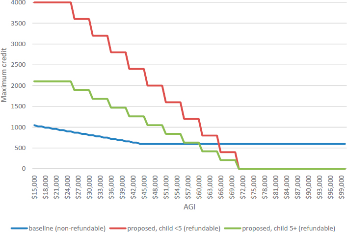
in the CPS-ASEC appears lower than captured in other surveys.15 For this analysis, we did not impose any procedures to augment the reported amounts. To the extent that the survey underidentifies the incidence or amount of child care expenses for lower-income families, the relative impact of the policy changes could be misestimated.
CCDF Policy: Implementation Assumptions
The federal government’s CCDF block grant provides money to states that they use to provide child care subsidies to lower-income families with children who are age 12 or under or who have a special need. The parents or guardians in the families must generally be employed, in school, or looking for work. One key point about the current program is that the eligibility limits vary by state. States may set the limits no higher than 85 percent of state median income; most states’ limits are lower. A second key point is
___________________
15 The CY 2015 CPS-ASEC captures $48.2 billion in child care expenses, compared with $59.0 billion in annual expense according to the National Survey of Early Care and Education (NSECE), which was fielded in 2012. (The NSECE figure was tabulated by TRIM3 project staff from the publicly available microdata; it is the average weekly aggregate amount from the data, times 52.)
that the subsidies are not an entitlement. The number of families receiving a subsidy in the average month of 2015—834,000—is about 17 percent of the total estimated by TRIM3 as being eligible for the subsidies. Some portion of the eligible families who do not receive CCDF-funded subsidies are receiving other types of help, such as TANF-funded child care, Head Start or state-funded pre-kindergarten, and others may not want or feel that they need assistance. However, some portion of the unassisted eligible families may be unable to receive subsidies due to funding constraints in their state or locality.
The Committee’s proposed change to CCDF is to guarantee assistance to all families with income below 150 percent of poverty who want the subsidy, implicitly assuming that funding would increase as needed to pay for the additional subsidies. To simulate this policy, we made the following assumptions regarding eligibility, copayments, and the value of the subsidy:
- In states with baseline eligibility limits below 150 percent of the 2015 poverty guidelines, the limits were raised to exactly equal 150 percent of poverty, for each family size. States with baseline eligibility limits higher than 150 percent of poverty were assumed to continue using those higher limits. (The modeling captured the fact that Alaska and Hawaii have higher poverty guidelines than the 48 contiguous states and the District of Columbia.)
- All other eligibility-related policies—such as the definition of the family unit, whether or not specific types of income are considered in determining eligibility, and whether a parent must work a minimum number of hours per week to be considered eligible based on employment—were all assumed to remain at the baseline settings in each state. (These policies vary across the states.)
- All policies related to copayments and reimbursement rates were also assumed to remain at each state’s baseline settings.
Assumptions also had to be made regarding enrollment—the extent to which eligible families who are guaranteed a subsidy under the hypothetical policy would choose to receive a subsidy. We assumed that families with income under 150 percent of the poverty guideline who did not receive a subsidy in the baseline simulation would start to receive a subsidy only if they reported child care expenses in the CPS-ASEC survey. This conservative assumption regarding take-up ensured that no families would become worse-off financially as measured by the SPM measure. (If a family with no baseline child care expenses had been modeled to begin to receive a subsidy and to owe a positive copayment, the SPM measure would show that family as worse-off financially, since the SPM considers child care expenses as a subtraction from resources, rather than considering the value of the subsidy
as an addition to resources.) Since many lower-income working families do not report having any child care expenses, this assumption minimized the number of new recipients according to the simulation. No changes in participation were modeled for families with income approximately 150 percent of poverty.
In families simulated to begin receiving a subsidy, assumptions also need to be made about the type of care they would choose for their children (child care center, family day care home, or informal care) since those choices affect the cost of the new subsidies (and in some states also affect the family’s copayment). We assumed that the percentage distribution of the newly subsidized children across different types of child care providers would be the same as distribution of currently subsidized children in the same age group and state of residence.
Child Care Expense Policy: Employment and Earnings Effects
The Committee assumed that both of the hypothetical policies related to child care expenses would increase maternal employment by reducing the effective cost of child care. Blau (2003) summarized the results of numerous studies showing the relationship between the price of child care and maternal employment. The Committee chose a price elasticity of 0.2 as being the approximate midpoint across a group of studies viewed as most applicable. With an elasticity of 0.2, a 10 percent reduction in the net price of child care causes a 2 percent increase in the employment rate.
For each of the child care expense simulations, the price elasticity was used to compute a target for increased employment. The first step in this computation was to compute estimates of aggregate net out-of-pocket child care expenses under different assumptions, for the universe of women who are working in the baseline (prior to any policy changes). For both unmarried mothers of children age 12 and under and married mothers of children age 12 and under, three aggregate amounts were computed: aggregate net child care expenses in the baseline, aggregate net child care expenses with the CDCTC policy in place, and aggregate net child care expenses with the CCDF policy in place. Aggregate net child care expenses were defined as aggregate child care expenses (including unsubsidized expenses plus the copayments paid by subsidized families), minus the aggregate amount of federal CDCTC, minus the aggregate amount of state-level CDCTC. For each of the two policies, we compared the aggregate net out-of-pocket expenses with the policy in place to the aggregate net out-of-pocket expenses in the baseline to determine the percentage reduction in net expenses. The absolute value of the percentage change was multiplied by 0.2 to obtain the percent increase in employment for each marital status, for each policy. The percentage
changes were multiplied by the numbers of currently employed mothers to obtain the targets for increased employment.
The CDCTC policy caused substantial reductions in out-of-pocket child care expenses for unmarried mothers of children age 12 and under, reducing the aggregate level of those expenses by 42.6 percent (see Table CC-1). (For some individual women, expenses were reduced by 100 percent, since the credit percentage was 100 percent for the lowest-income mothers of young children.) For married women, however, the CDCTC policy increased aggregate expenses, due to the fact that tax units with AGI above $75,000 lost the CDCTC, and most of those units were married couples. Applying the elasticity to the percentage changes in aggregate expenses and to the baseline numbers of employed mothers resulted in targets of 607,000 newly working unmarried mothers and a decline in employment of 128,000 for married mothers.
The CCDF policy was estimated to have a smaller impact on aggregate child care expenses, reducing expenses by 16.6 percent among currently working unmarried mothers and by 0.6 percent for married mothers. Those changes resulted in estimates of 237,000 newly-working unmarried mothers and 15,000 newly-working married mothers.
To assign the new jobs, it was necessary to identify which women would benefit from the new policies if they began to work. Three preliminary simulations were performed in which currently nonworking women were modeled to begin to work, using the same distribution of job characteristics
TABLE CC-1 Changes in Maternal Employment due to Child Care Expense Policies
| Child Care Policy #1: CDCTC Expansion | Child Care Policy #2: CCDF Expansion | |
|---|---|---|
| Unmarried Mothers of Children <= 12 (7.119 Million Employed in Baseline) | ||
| Percent Reduction in Aggregate Child Care Costs | 42.6 percent | 16.6 percent |
| Multiplied by Elasticity of 0.2 | .085 | .033 |
| Targeted Increase in Employment | 607,000 | 237,000 |
| Married Mothers of Children <= 12 (13.183 Million Employed in Baseline) | ||
| Percent Reduction in Aggregate Child Care Costs | Neg. 4.9 percent | 0.6 percent |
| Multiplied by Elasticity of 0.2 | -.010 | .001 |
| Targeted Increase in Employment | -128,000 | 15,000 |
and hourly wages as used for the EITC simulation (Table EITC-3). The three simulations used three different sets of policy rules:
- Baseline policies for both CDCTC and CCDF. In this simulation, all newly employed mothers are assumed to have to pay for child care. A regression equation predicts the amount of expense based on family characteristics and the children’s ages. (The equation was calibrated to produce the same average nonzero expense amounts as reported in the survey data, by AGI level.) We assume none of the new workers can receive CCDF; however, they take the CDCTC if they are eligible.
- Hypothetical CDCTC policy. This simulation is the same as #1, but the federal CDCTC policy is the Committee’s proposed expanded policy.
- Hypothetical CCDF policy. This simulation is the same as #1, but the CCDF policy is the same as the Committee’s proposed expanded policy. This simulation identifies which women, when they start to work, are guaranteed a subsidy.
The new jobs due to the CDCTC policy were assigned randomly among the subset of the unmarried mothers who were identified as better off in the second preliminary simulation (in which they start to work and must pay for child care, but the new policy is in place) compared with the first preliminary simulation (in which they start to work and must pay for child care, but the CDCTC is at baseline levels).
The new jobs due to the CCDF expansion were assigned to a subset of women—both unmarried and married—who are guaranteed a subsidy when they start to work under the new policy.
For the CDCTC policy, the job reductions for married women were assigned randomly among the subset of married mothers who were worse-off under the new policy than the baseline policy, when the new CDCTC policy was modeled without employment changes.
Child Care Expense Policy: Simulation Results
In the absence of employment effects, the two policies focused on child care expenses resulted in relatively modest reductions in child poverty. In both cases, the assumptions about employment changes caused additional reductions in poverty.
The CDCTC expansion, prior to employment changes, causes federal tax liability to decline by $1.6 billion (Table CC-2). State tax liability also declines, due to the state income tax credits that are calculated based on the amount of federal credit. The reductions in tax liability reduce children’s
TABLE CC-2 Selected Impacts of Child Care Expense Policy Changes, 2015
| Baseline 2015 | Changes from the Baseline | ||||
|---|---|---|---|---|---|
| Child Care Policy #1: Expansion of CDCTC | Child Care Policy #2: Expansion of CCDF | ||||
| No EE | With EE | No EE | With EE | ||
| Number of Children in SPM Poverty (Millions) | 9.633 | -0.198 | -0.872 | -0.109 | -0.427 |
| SPM Child Poverty Ratea | 13.0% | -0.3 | -1.2 | -0.1 | -0.6 |
| Selected Program Results | |||||
| Child Care Subsidies | |||||
|
Families Eligible for Child Care Subsidies (Avg. Mo., Thousands) |
5,016 | 340 | 303 | 516 | |
|
Families Receiving Child Care Subsidies (Avg. Mo., Thousands) |
834 | 807 | 1,019 | ||
|
Aggregate Annual Value of Subsidy ($ Millions) |
$6,611 | $6,228 | $7,936 | ||
| Federal income taxes | |||||
|
Amount of Tax Liability ($ Millions) |
$1,254,515 | -$1,606 | -$7,462 | $6 | -$1,166 |
| State income taxes | |||||
|
Amount of Tax Liability ($ Millions) |
$318,089 | -$210 | -$699 | $40 | -$15 |
|
Employment and Earnings Changes |
|||||
|
People Who Start Working (Thousands) |
0.600 | 0.250 | |||
|
People Who Stop Working (Thousands) |
0.130 | 0.000 | |||
| Net Annual Earnings Change ($ Millions) | $4,699 | $4,492 | |||
| Spending and Tax Summary ($ Millions) | |||||
| Aggregate Benefits Paidb | $197,816 | $0 | -$2,171 | $5,891 | $6,407 |
| Aggregate Taxes: Payroll, Federal, State | $2,588,958 | -$1,816 | -$7,313 | $46 | -$487 |
| Total Change, Annual Government Spending | $1,816 | $5,141 | $5,845 | $6,894 | |
NOTE: EE = Employment Effects.
a Changes are shown in percentage points.
b The benefit programs included in these figures are unemployment compensation benefits, SSI, TANF, child care subsidies, housing subsidies, SNAP, LIHEAP, and WIC.
SPM poverty rate by 0.3 percentage points. Despite the large increase in the amount of the CDCTC, and the fact that it becomes fully refundable, the policy still only has the potential to raise a family out of SPM poverty if the family has child care expenses, and many lower-income families do not report any child care expenses. For example, in the CY 2015 CPS-ASEC data, among families with employed parents/guardians, children age 12 and under, and AGI of $25,000 or less, only about 30 percent reported any positive child care expenses.
The employment effects increase the anti-poverty impacts of the CDCTC expansion. When the CDCTC policy is modeled together with 600,000 unmarried women starting to work, and 130,000 married women leaving their jobs, the impact of the new jobs predominates, and child SPM poverty falls by 1.2 percentage points from the baseline (to 11.8%). The reduction in federal tax liability relative to the baseline is $7.5 billion, since all of the new workers are benefiting from the CDCTC, and most are also receiving the EITC. Note that although many of the new workers become eligible for CCDF subsidies (increasing the average monthly number of families eligible for CCDF by 340,000), we assumed that none of them would receive CCDF subsidies; instead, we assumed that if CCDF subsidies had actually been an option for these women, they would have begun to work previously.
The CCDF expansion, prior to employment changes, causes 303,000 additional families to be eligible for child care subsidies (because state income limits below 150 percent of poverty in the baseline were raised to that level) and causes 807,000 families to newly receive CCDF subsidies. However, the number of children in SPM poverty was reduced by only 109,000—a drop of 0.1 percentage point in the SPM poverty rate for children. One reason for the limited anti-poverty impact of the CCDF policy is that, in some cases, the family copayment required by the CCDF program was almost as high as the amount of unsubsidized expense the family paid in the baseline. (For a single parent with earnings of $20,000 and a twoyear-old child in full-time center-based care, the median copayment in 2015 was $117 per month—or $1,404 per year.16)
When the CCDF expansion is modeled together with 250,000 new jobs, the number of families eligible for CCDF in the average month of the year increases by 213,000 relative to the simulation without employment increases. (The increase in average monthly eligibility is less than the 250,000 increase in employed mothers because some of the newly employed women are ineligible for CCDF in some months of the year for various reasons, such as a spouse being out of the labor force in those months.) All of the families newly eligible for CCDF take the subsidy. Even though
___________________
16 See Stevens et al., 2016, Table 31.
most of these families must pay a copayment, the copayment is much less than the amount of their new earnings. Also, most of the new workers can also claim the EITC; federal income tax liability declines by $1.2 billion relative to the baseline when the CCDF expansion is modeled together with the employment increases. Combining all of these changes, children’s SPM poverty falls by 0.6 percentage points relative to the baseline.
MINIMUM WAGE
Since 2009, the federal minimum wage for most workers has been set at $7.25 per hour. The federal minimum wage for tipped workers is $2.13. The Committee requested two simulations of minimum wage increases:
- Minimum Wage Policy #1: An increase in the federal minimum wage to $10.25 in 2020 dollars, in all states. The figure of $10.25 was deflated to $9.15 for purposes of the simulations, for consistency with the dollars of the input data.17 This results in an increase of 26.2 percent in the 2015 minimum wage. The same minimum wage was assumed to be applied in all states, except that states with a minimum higher than $9.15 in 2015 were assumed to keep their 2015 minimum wage. The federal tipped minimum wage is assumed to increase by the same percentage as the regular minimum wage, bringing it to $2.69 per hour. As with the regular minimum wage, states with higher state levels for their tipped workers retain those higher minimums.
- Minimum Wage Policy #2: This policy is the same as Minimum Wage #1, with one exception. In this variation, the new value for the regular minimum wage in each state equals the lesser of $9.15 or the 10th percentile of the hourly earnings distribution in that state.
To model these policies, information was obtained on each state’s actual minimum wages in 2015—for most workers and for tipped workers—as well as the 10th percentile of each state’s hourly earnings distribution (Table MW-1). Four states—Connecticut, Oregon, Vermont, and Washington—and the District of Columbia had minimum wages higher than $9.15 in 2015, and were therefore largely unaffected by the minimum wage policies.
___________________
17 The most recent Congressional Budget Office estimate of the 2020 Consumer Price Index, All Urban Consumers (CPI-U) at the time this work began (CBO, 2017) was 262.8, 11 percent higher than the actual 2015 CPI-U of 237.0. Applying those estimates to the 2020 minimum wage proposal of $10.25 would result in a 2015 value of $9.24; the Committee specified a slightly lower value of $9.15. (CBO forecasts are available on the CBO website, https://www.cbo.gov/about/products/budget-economic-data.)
TABLE MW-1 State-level Minimum Wage Data, 2015
| State | Regular Minimum Wage ($) | Tipped Minimum Wage ($) | 10th Percentile Wage ($) | State | Regular Minimum Wage ($) | Tipped Minimum Wage ($) | 10th Percentile Wage ($) |
|---|---|---|---|---|---|---|---|
| Alabama | 7.25 | 2.13 | 8.36 | Missouri | 7.65 | 3.83 | 8.63 |
| Alaska | 8.75 | 8.75 | 10.62 | Montana | 8.05 | 8.05 | 8.91 |
| Arizona | 8.05 | 5.05 | 8.96 | Nebraska | 8.00 | 2.13 | 8.95 |
| Arkansas | 7.50 | 2.63 | 8.31 | Nevada | 7.25 | 7.25 | 8.67 |
| California | 9.00 | 9.00 | 9.48 | New Hampshire | 7.25 | 3.26 | 9.08 |
| Colorado | 8.23 | 5.21 | 9.21 | New Jersey | 8.38 | 2.13 | 9.33 |
| Connecticut | 9.15 | 5.78 | 9.63 | New Mexico | 7.50 | 2.13 | 8.62 |
| Delaware | 8.25 | 2.23 | 9.10 | New York | 8.75 | 4.90 | 9.33 |
| Dist. of Col. | 10.50 | 2.77 | 11.49 | North Carolina | 7.25 | 2.13 | 8.52 |
| Florida | 8.05 | 5.03 | 8.82 | North Dakota | 7.25 | 4.86 | 9.70 |
| Georgia | 7.25 | 2.13 | 8.46 | Ohio | 7.25 | 4.05 | 8.90 |
| Hawaii | 7.75 | 7.25 | 9.23 | Oklahoma | 7.25 | 2.13 | 8.49 |
| Idaho | 7.25 | 3.35 | 8.52 | Oregon | 9.25 | 9.25 | 9.71 |
| Illinois | 8.25 | 4.95 | 9.17 | Pennsylvania | 7.25 | 2.83 | 8.80 |
| Indiana | 7.25 | 2.13 | 8.57 | Rhode Island | 9.00 | 2.89 | 9.40 |
| Iowa | 7.25 | 4.35 | 8.70 | South Carolina | 7.25 | 2.13 | 8.38 |
| Kansas | 7.25 | 2.13 | 8.69 | South Dakota | 8.50 | 4.25 | 9.17 |
| Kentucky | 7.25 | 2.13 | 8.51 | Tennessee | 7.25 | 2.13 | 8.49 |
| Louisiana | 7.25 | 2.13 | 8.35 | Texas | 7.25 | 2.13 | 8.55 |
| Maine | 7.50 | 3.75 | 9.07 | Utah | 7.25 | 2.13 | 8.78 |
| Maryland | 8.25 | 3.63 | 9.10 | Vermont | 9.15 | 4.58 | 10.05 |
| Massachusetts | 9.00 | 3.00 | 9.87 | Virginia | 7.25 | 2.13 | 8.83 |
| Michigan | 8.15 | 3.10 | 8.99 | Washington | 9.47 | 9.47 | 10.63 |
| Minnesota | 7.25 | 7.25 | 9.28 | West Virginia | 8.00 | 2.40 | 8.63 |
| Mississippi | 7.25 | 2.13 | 8.26 | Wisconsin | 7.25 | 2.33 | 8.75 |
| Wyoming | 7.25 | 2.13 | 9.19 |
Twenty-nine states used minimum wages for tipped workers in 2015 that were higher than $2.69; the highest minimum wage for tipped workers was $9.47, in the state of Washington (with the same wage for tipped and nontipped workers). In 33 states, the 10th percentile of the 2015 hourly wage distribution was lower than $9.15; in these 33 states, the simulated minimum wage in the Minimum Wage #2 policy was lower than $9.15. The lowest figure for the 10th percentile of the 2015 hourly wage distribution was $8.26, in Mississippi.
Minimum Wage Policy: Implementation Assumptions Concerning Wage Increases
For a given individual identified as receiving a wage increase due to an increase in the minimum wage, the modeling of the policy is straightforward. For example, if a person works full time, full year at $8.15/hour, the increase to $9.15/hour increases his or her monthly earnings by $173 ($1 times 40 hours per week times 4.333 weeks in a month). Computationally, the model computes the percentage increase from a person’s original hourly wage to the new hourly wage, and then it applies that percentage increase to the person’s monthly and annual earnings amounts.
However, complications arise in determining current hourly wages, identifying which workers might be affected by the increase, modeling some additional wage increases that might occur even if not legislatively required (sometimes called “spillover” increases), modeling changes for workers receiving the tipped minimum wage, and modeling changes for other tipped workers. Decisions in these areas were reached jointly between Urban Institute and Committee staff.
Computing Current Hourly Wages
The hourly wages we use to implement the minimum wage increase come from two sources: explicitly reported wages from the CPS “earnings sample” (ES) data, and estimated hourly wages computed from annual CPS-ASEC data. The monthly CPS questionnaire asks people to report their exact hourly wage at the time of the survey if they are in the “earnings sample”—people in their 4th or 8th month of participation with the CPS (also referred to as the outgoing rotation group); thus, the CPS-ASEC for CY 2015 includes hourly wages only for those CY 2015 earners who were in their 4th or 8th month of CPS participation in the month in which the ASEC questions were administered, and who were also working in that month. To maximize the number of people with these data, we also obtain the ES data from other monthly CPS files to the extent it is available. However, even after that additional information is obtained, usable ES data
are not available for many CY 2015 workers, either because the person was working during the CY but not working in the month when the wage question was asked, or because the person’s identification number is not located in the monthly CPS when the person should have been asked the ES questions (due to attrition from the sample or due to matching problems).
The second possible source of hourly wage data is to compute the wage from annual ASEC data. Specifically, we compute an hourly wage as (annual earnings) divided by (weeks of work times usual hours per week). Of course, this gives an imperfect hourly wage, since any inaccuracy in the reporting of any of the three pieces of information will mean an inaccurate wage. On net, those inaccuracies tend to result in a distribution with too many very-low-wage workers, relative to wage distributions based solely on outgoing-rotation-group data.
For each person with CY 2015 earnings, the ES hourly wage is generally used when it is available. However, the ES wage is not used in two situations. First, if the ES wage was “allocated” (imputed by the Census Bureau) and the annual earnings, weeks of work, and hours per week were all truly reported, then the hourly wage computed from the annual data is used instead. Second, if the person’s CY 2015 annual earnings divided by the ES hourly wage indicates that it would take more than two full-time full-year jobs to earn that level of earnings at the given hourly wage, that suggests that the person changed jobs between the calendar year and the outgoing month; in that case, the wage computed from the annual data is used instead of the ES wage. The hourly wage computed from the annual data is also used in all cases when an ES wage is not available.
Identifying Workers Covered By the Regular Minimum Wage
In general, we identify workers covered by the standard minimum wage (not the tipped minimum) as those whose hourly wage (determined as described above) is no more than 25 cents below the larger of the federal minimum wage or their state’s minimum wage. (See the first column of Table MW-1 for state-specific minimum wage levels.) This use of a “tolerance” for identifying minimum wage workers compensates for the fact that some people who are true minimum wage workers might have a slightly lower computed wage due to rounding of some element of their annual data. For example, in a state that does not have a minimum wage higher than the federal minimum, workers with hourly wages between $7.00 and $9.14 would be directly affected by an increase in the minimum wage to $9.15. This approach does not attempt to apply the rules regarding jobs exempt from minimum wage laws (including seasonal workers, informal workers, some workers with disabilities, and others); we implicitly assume that those workers would either have an hourly wage below the cutoff that
is considered affected by the minimum age, or that their wages might be affected even if that would not be legally required. Also, we did not model any wage increases for workers with both wage or salary income and self-employment income, due to challenges in computing hourly wages for individuals with both types of earnings.
Modeling Spillover Increases
Estimates of the impact of minimum wage increases generally assume that employers would increase the wages of some employees beyond what is legislatively required. This could occur when an employer wants to maintain a certain relative ordering of hourly wages across a group of employees. For example, if the employer currently has employees making $7.25, $9.00, and $9.75, and the minimum wage increases to $9.15, the employer would be required to raise the wages of the two lower-paid employees to $9.15. The employer might choose to raise the second employee’s wages to something higher than $9.15 so that person continues to earn more than the person who previously earned $1.75 less; in that case, the employer might also choose to somewhat raise the wages of the person making $9.75.
The Committee requested that we follow the approach of the Congressional Budget Office’s minimum wage analysis (CBO, 2014) in estimating these types of spillover increases. Specifically, in the CBO analysis (CBO, 2014, p. 29), “Ripple effects were included for workers whose wages under current law were projected to be slightly less and slightly more than the minimum wages under each option.” Regarding people with baseline wages slightly more than the new minimum wage, CBO assumed (CBO, 2014, p. 21) that a person would get some wage increase if the person’s current wage is “up to the amount that would result from an increase that was 50 percent larger than the increase in their effective minimum wage (incorporating both their state minimum and the new federal minimum) under either option.” Considering a state that uses the federal minimum wage of $7.25, the effective minimum wage increase being applied in the 2015 data is $1.90; 50 percent of that amount is $0.95, resulting in a wage of $10.10. Thus, spillover increases would occur for workers with baseline wages up to $10.10. The CBO report was not as specific regarding the treatment of workers with baseline wages slightly below the new minimum; in the absence of that information, project staff and Committee members agreed that the spillover area below the new minimum should have the same width. Thus, for a state using the federal minimum wage, spillover increases occur from $8.20 (95 cents below the new minimum) to $10.10 (95 cents above the new minimum). The spillover ranges were modified for states with higher minimum wages. For example, in Arizona, which used an $8.05 minimum wage, the spillover increases occurred from $8.60 to $9.70.
For workers with a baseline wage above the new minimum, but below the ending point of the spillover range, the new wage equals the new plus an additional amount, computed as follows: the gap between the current wage and the starting point of spillover in their state multiplied by 0.5. For example, in the case of a worker earning $9.00 in a state with a $7.25 minimum, the new wage equals $9.15 plus an additional increase of $0.40—computed as (($9.00-$8.20) * 0.5)—giving a final new wage of $9.55. The relationship between the new required wages and the wages including the spillover assumptions is shown in Figure MW-1 for a state using the federal minimum wage.
Modeling Changes for Workers Who Receive the Tipped Minimum Wage
Workers in some occupations that receive a large portion of their compensation in tips often receive what is known as the “tipped minimum wage,” currently set at $2.13 at the federal level and higher in some states. Based on data on median hourly base pay, we treat the following
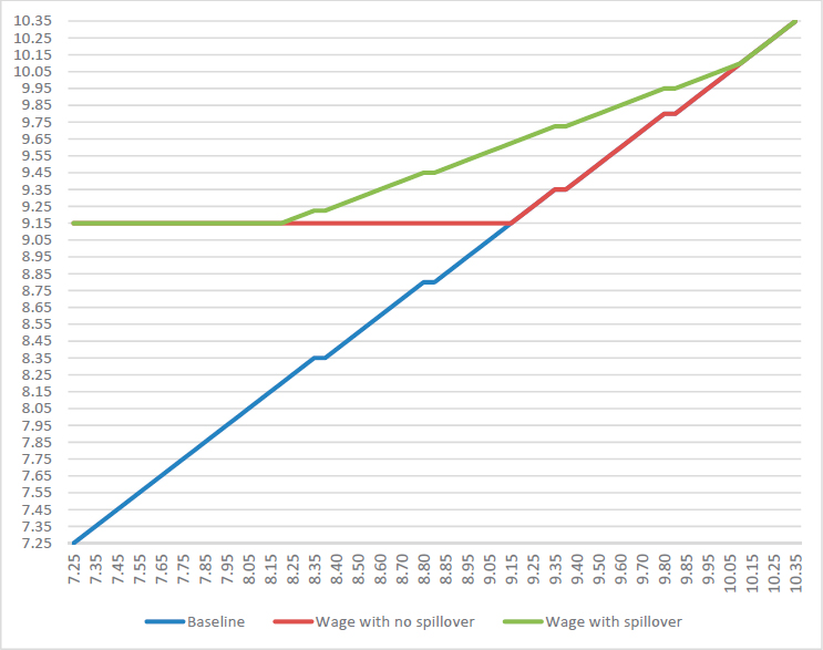
occupations as receiving the tipped minimum wage: waiters, bartenders, gaming service workers, and dining room and cafeteria attendants.18 Under the tipped minimum wage, the employer is required to pay only that tipped minimum as long as the worker’s tips bring his or her total compensation to at least the regular minimum wage; if not, the employer is required to pay additional wages to raise the total to the regular minimum. For example, in a state using the federal levels of $2.13 for the tipped minimum and $7.25 for the regular minimum, as long as the employee receives at least $5.12 per hour in tips, the employer need only pay the tipped wage of $2.13 per hour.
How a worker making the tipped minimum wage is affected by an increase in the tipped and regular minimum wage amounts depends on the worker’s current total hourly pay (including tips) relative to the tipped minimum wage, the current regular minimum wage, and the new minimum wage. As mentioned above, values up to 25 cents below the regular minimum are assumed to be at the regular minimum; similarly, values up to 13 cents below the tipped minimum are assumed to be at the tipped minimum. To obtain that total pay, for this group of workers we rely solely on the hourly wages computed from the CPS-ASEC annual data, which include tips as well as base pay. (The ES wages exclude tips.) Wages are modified for workers assumed to be receiving the tipped minimum wage as follows:
- When total hourly pay is below the current regular minimum wage (range of $2.00 to $7.00 in a state with federal minimum wage values): If a worker’s estimated total hourly pay is within the range from 13 cents below the state’s tipped minimum wage to 26 cents below the state’s regular minimum, we assume the employer was not complying with the minimum wage law, and would continue to not comply. Therefore, for these workers, wages are increased by only the amount of the tipped minimum wage increase. In a state with the federal values, this is an increase of 56 cents per hour; if the state’s tipped minimum already exceeds $2.69, no increase is modeled.
- When total hourly pay is between the current regular minimum and the new minimum (range of $7.00 to $9.15 in a state with federal minimum wage values): In this situation, either the employer is bringing the employee’s total pay up to the current minimum, or the employee is making more than the current minimum due to
___________________
18 In data developed by the compensation research firm PayScale (https://www.payscale.com/tipping-chart-2012) the median hourly base pay (excluding tips) in these occupations in 2012 was below $8.00 ($5.10 for waiters, $7.60 for gaming services workers, and $7.70 for both bartenders and for dining room and cafeteria workers). For all other occupations identified as receiving substantial levels of tips (e.g., hairdressers), median hourly base pay exceeds $8.00, indicating that these occupations generally receive tips in addition to a regular wage of at least the minimum wage.
- tips. We increase these workers’ wages to exactly the regular minimum wage; since we do not have any evidence to the contrary, we assume that the employers in these cases would add sufficient base pay to raise the total hourly pay to the new minimum.
- When total hourly pay is equal to or higher than the new minimum (hourly pay of $9.15 or above): We assume workers in one of the tipped-minimum-wage occupations who already have total pay above the new minimum are making substantial tips. However, they would still benefit from the increased tipped minimum. We increase these workers’ wages by the amount of the tipped minimum wage increase, which is 56 cents per hour in the states with the federal wage values.
Modeling Changes for Other Workers Who Receive Tips
In addition to workers who receive the tipped minimum wage, many other workers receive tips in addition to receiving a base pay amount that is at least as high as the regular minimum wage. We consider the following occupations as receiving tips, but not the tipped minimum wage: barbers, hairdressers, other personal appearance workers, massage therapists, hosts and hostesses, taxi and chauffer drivers, and all other person care and service workers.19
For this group of workers, estimating the impact of the minimum wage increase requires not only an estimate of the total hourly pay including the tips, but also the amount of base pay vs. tips. As with the modeling of the workers receiving the tipped minimum, the modeling for this group uses the hourly wages computed from the annual data rather than the ES wages as the combined amount of base pay and tips. The hourly base pay is estimated as that person’s total pay minus the median value of hourly tips for the person’s occupation.20
The impact of the new minimum wage on this group of workers depends on their estimated hourly wage without tips relative to the new minimum wage.
If the estimated wage without tips is more than 25 cents below the current minimum, we assume the person is not covered by the minimum wage law (the same assumption made for nontipped workers) and no changes are made.
___________________
19 This list of occupations includes all those listed as predominantly tipped occupations in an analysis by Allegretto and Cooper (2014) other than those considered to receive the tipped minimum wage.
20 The median hourly tips for these occupations range from $1.90 for hosts and hostesses to $5.30 for taxi drivers and chauffeurs. The data were collected by the compensation research firm PayScale in a 2012 survey; see https://www.payscale.com/tipping-chart-2012.
If the estimated wage without tips is between the current minimum (with the 25-cent tolerance) and the new minimum, the new base wage equals the new minimum. (For simplicity, no spillover increases were modeled for this group.) The person’s new total wage equals the new base wage plus the estimated value of hourly tips, which are assumed to be unchanged. (If customers reduce their tips when the minimum wage increases, then we are overestimating the total pay increase for this group.)
If the estimated wage without tips exceeds the new minimum, the person’s wages are unchanged.
Minimum Wage Policy: Employment Effects
The Committee assumed that increases in the minimum wage would cause some reduction in employment; they requested that the simulations follow the job-reduction approach used by CBO (2014) as closely as possible.
The CBO’s approach derives separate targets for the reduction in employment for teenagers and adults. The starting point for the process is the identification of a single estimate for teenagers of the elasticity of job loss due to a minimum wage increase; for an increase of $9.00, the CBO researchers reviewed the literature and identified -0.075 as the most appropriate starting estimate. Since the increase estimated here is very close to $9.00, we begin with the same teen-worker elasticity. This suggests that, across all teen workers, employment falls by 0.75 percent due to a 10 percent increase in the minimum wage, or by 1.97 percent due to the 26.2 percent increase in the minimum wage enacted in this policy.
However, the CBO procedures make two adjustments to that estimate so that it is more appropriate to apply in a microsimulation context. First, to make the elasticity applicable to directly affected teenagers—estimated to comprise about one-third of all teen workers in the period covered by the reviewed literature—the figure is divided by one-third; this gives a revised elasticity of -0.225. Second, CBO adjusts the elasticity to apply to the wage change that is required to reach the new minimum—which is less than the full change in the minimum wage since many affected workers are already making above the current minimum wage. Because the full increase was observed by CBO to generally be about 50 percent higher than the wage increases required for compliance, the elasticity is multiplied by 1.5, for a final elasticity of 0.3375. For adults, the CBO estimated that the elasticity would be one-third the size of the elasticity for teens, or 0.1125.
Based on discussion with the Committee members, we used these elasticities to estimate the targeted number of lost jobs, creating separate estimates for teens and adults. For each age group, we calculated the mean percent change in wages for all those directly affected by the wage increase.
(The directly affected group excludes those whose only increase is due to spillover.) In the simulation of Minimum Wage Policy #1, the average hourly wage increases for this group were 13.8 percent for teens and 11.9 percent for adults (Table MW-2). Multiplying these percentages by the elasticities produces estimates that employment will fall by 4.7 percent among directly affected teens and by 1.3 percent among directly affected adults due to the minimum wage increase. When applied to the universe of directly affected teens and adults, these percentages generate targets for job loss of 28,000 among directly affected teens and 121,000 among directly affected adults due to Minimum Wage Policy #1. For Minimum Wage Policy #2, the estimated average wage increases and targeted job losses are somewhat lower.
The targeted employment reduction was achieved by randomly selecting workers to stop working, from among all those workers who were directly affected by the minimum wage policy. In other words, a teenager with a current hourly wage of $7.25 and a teenager with a current hourly wage of $9.10 both had the same likelihood of job loss. The Committee chose this approach rather than an approach giving different likelihoods of job loss depending on a person’s starting wage, since the available evidence does not specifically address the relative likelihoods of job loss depending on a worker’s starting wage.
For each age group, the job loss was distributed proportionally across three broad groups of workers—nontipped workers, workers receiving the tipped minimum wage, and other tipped workers—in the same proportions
TABLE MW-2 Key Data for Estimates of Employment Reduction Among Workers Directly Affected by a Minimum Wage Increase
| Minimum Wage Policy #1 | Minimum Wage Policy #2 | |||
|---|---|---|---|---|
| Teen Workers | Adult Workers | Teen Workers | Adult Workers | |
| Elasticity, Adjusted to Apply to Average Increase in Wage for Directly Affected Workers | -0.3375 | 0.1125 | -0.3375 | 0.1125 |
| Average Increase in Wage | 13.8% | 11.9% | 10.5% | 9.2% |
| Average Increase * Elasticity = Estimated Percent Employment Change for Directly Affected Workers | -4.7% | -1.3% | -3.5% | -1.0% |
| Directly Affected Workers | 604,000 | 9,002,000 | 556,000 | 7,038,000 |
| Targeted Employment Change = Percent Change Times Number Directly Affected Workers | -28,000 | -121,000 | -20,000 | -73,000 |
as those groups comprised of the entire group of directly affected workers. For example, because about 83 percent of directly affected adults are not in tipped occupations, about 83 percent of the job loss for adults also occurs among nontipped directly affected adults.
Because this job loss was assumed to be involuntary, all the individuals modeled to lose their jobs were assumed to receive unemployment compensation for 26 weeks, offsetting a portion of the impact of the lost wages. Because some portion of people losing their jobs would likely be ineligible for unemployment compensation (due to insufficient work history to meet their state’s requirements), the receipt of unemployment compensation in this simulation is probably overstated.
Minimum Wage Policy: Simulation Results
The minimum wage policy changes reduced child SPM poverty slightly—from 13.0 percent to 12.8 percent (Minimum Wage Policy #1) or 12.9 percent (Minimum Wage Policy #2).
Results Prior to Employment Loss
The initial simulations of the minimum wage policies included direct wage increases and spillover effects, but no job loss. (See the columns labeled “No EE” in Table MW-3). Prior to the simulation of any job loss, Minimum Wage Policy #1 provides increased wages for 14.5 million workers, and Minimum Wage #2 increases wages for 10.3 million workers. In aggregate, wages increase by $13.9 billion and $8.0 billion, respectively. The impacts in Minimum Wage #2 are smaller because, in the 33 states in which the 10th percentile of the wage distribution is lower than $9.15, the increase in the minimum wage is not as large as it is in Minimum Wage #1.
Considering the number of people who receive a raise from the simulated increases in the minimum wage, it is initially surprising that the anti-poverty impacts are not larger. The relatively modest anti-poverty impacts are due to two main factors. First, only a portion of the affected workers are in low-income families with children. For example, in the implementation of Minimum Wage Policy #1, among the total 14.5 million workers who receive a raise, only 0.8 million are in families meeting two key criteria—having children under age 18 and having baseline family resources less than 100 percent of the SPM poverty threshold. All the other people who receive a wage increase are either in families without children or in families that are not low-income according to the SPM definition. Second, among the 0.8 million workers receiving a wage increase who are in families in SPM poverty with children under 18, only 42 percent (342,000) work both full time and full year during CY 2015; for the others, the
TABLE MW-3 Selected Impacts of Minimum Wage Policy Changes, 2015
| Changes from the Baseline | |||||
|---|---|---|---|---|---|
| Minimum Wage Policy #1: Increase to $9.15 in 2015 Dollars | Minimum Wage Policy #2: Increase to 10th Percentile Wage or $9.15, Whichever Is Less | ||||
| Baseline 2015 | No EE | With EE | No EE | With EE | |
| Number of Children in SPM Poverty (Millions) | 9.633 | -0.128 | -0.121 | -0.065 | -0.059 |
| SPM Child Poverty Ratea | 13.0% | -0.2 | -0.2 | -0.1 | -0.1 |
|
People With Increased Earnings (Thousands, Working in Baseline) |
14.468 | 14.321 | 10.345 | 10.252 | |
|
People Who Stop Working (Thousands) |
0.000 | 0.147 | 0.000 | 0.093 | |
|
Net Annual Earnings Change ($ Millions) |
$13,867 | $12,624 | $7,997 | $7,227 | |
| Spending and Tax Summary ($ Millions) | |||||
|
Aggregate Benefits Paidb |
$197,816 | -$933 | -$78 | -$571 | $10 |
|
Aggregate Taxes: Payroll, Federal, State |
$2,588,958 | $3,950 | $3,609 | $2,226 | $2,031 |
|
Total Change, Annual Government Spending |
-$4,883 | -$3,688 | -$2,797 | -$2,021 | |
NOTE: EE = Employment Effects.
a Changes are shown in percentage points.
b The benefit programs included in these figures are unemployment compensation benefits, SSI, TANF, child care subsidies, housing subsidies, SNAP, LIHEAP, and WIC.
impact of the minimum wage increase on annual earnings is muted by the fact that they work part year and/or part time. Third, the increases in wages have secondary impacts on all the benefit and tax program included in these simulations. In the Minimum Wage Policy#1, for example, aggregate benefits fall by $0.9 billion due to the wage increases, and aggregate taxes increase by $4.0 billion. These secondary impacts lessen the anti-poverty impacts of the minimum wage increase. (For calculations showing how a minimum wage increase could affect a family’s benefits and taxes, see Acs et al., 2014.)
Results Including Employment Loss
When employment losses are included in the simulation, in addition to the other minimum wage impacts (the direct impacts, spillover increases, and secondary impacts on benefits and taxes), the reduction in child poverty is lessened by a very small amount, relative to the simulations without job losses. For example, in Minimum Wage Policy #1, the number of children raised out of SPM poverty is 128,000 without any job loss being modeled and 121,000 when job loss is modeled. As mentioned earlier, most of the people affected by the minimum wage increase were either not in families with children or not in families in SPM poverty; job loss has the potential to affect the child poverty results only for job-losers who are in poor families with children that would be raised out of SPM poverty by the minimum wage increase.
EMPLOYMENT POLICY
The Committee requested two simulations to approximate the implementation of a work training program—the WorkAdvance program—that has been implemented as a demonstration project and which appears to increase participants’ earnings (Hendra et al., 2016). The simulations assume that the WorkAdvance program has been operational for a number of years with a focus on low-income men who head households with children. The Committee requested two simulations, as follows:
- Work Program Policy #1: Assumes that 10 percent of men in the target group have received training under the program at some point prior to the year of the simulation.
- Work Program Policy #2: Assumes that 30 percent of men in the target group have received training under the program at some point prior to the year of the simulation.
Employment Policy: Implementation Assumptions
Simulating the WorkAdvance policy involved two initial steps before the earning effects could be imposed: identifying the potential universe and selecting the affected individual from within that universe.
Identifying the Potentially Affected Men
In the simulations, the WorkAdvance program is focused on men meeting all of the following criteria: the man is either unmarried and heading a household with children or part of a married couple heading a household with children; the cash income of the man’s family is below 200 percent of the official poverty threshold; the man is age 50 or younger; the man does not have a disability; the man is not a student; and the man is not an unauthorized immigrant. Regarding the last criterion, a report describing the WorkAdvance demonstration project (Tessler et al., 2014) states that participants were required to be legally authorized to work in the United States.
Selecting the Individuals Who Have Been Enrolled in the Program
The specific individuals identified as having received training under the program were selected to mimic the distribution of the demonstration program’s actual participants along two dimensions—educational attainment and recent employment history. Regarding education, 56 percent of the demonstration program participants had at least some college education and 44 percent had no more than a high school education or equivalent (see table 3.6 in Tessler et al., 2014).
Regarding recent work experience, men were classified in one of the following groups: either employed or not working for less than 1 month; not working for 1 to 6 months; or either not working for 7 or more months or never employed. These are the groups for which the evaluation provides separate estimates of impacts, as described further below. Based on the characteristics of the actual participants, we determined that among the simulated participants, 22 percent should be employed or have less than 1 month of nonwork during the year; 39 percent should have 1 to 6 months when they were not working during the year; and 39 percent should have 7 or more months during which they did not work during the year.21
___________________
21 These percentages are based primarily on table 3.5 in Tessler et al. (2014). However, that table grouped together participants unemployed for less than 3 months (without separate identification of those unemployed less than 1 month). We inferred that about 2 percent of enrollees were unemployed for less than 1 month. With that assumption, when the earnings impacts for the three employment subgroups are weighted by that subgroup’s estimated portion of the total (22, 39, and 39 percent), the resulting overall earnings impact equals the overall reported impact.
To come as close as possible to the desired characteristics, we first tabulated the universe of potential participants by education and by the three employment groups. Then, for each of the two options, we determined a set of probabilities for each combination of characteristics that would come as close as possible to achieving both the desired distribution by educational attainment and the desired distribution by weeks of work vs. nonwork. In the simulation in which 10 percent of the universe is assumed to have participated, the distribution of the simulated participants comes very close to the desired distributions (Table Work-1). For the simulation with 30 percent enrollment, the alignment is not quite as close; the number of men with 1 to 6 months of nonwork was not sufficient to reach the target for this simulation.
Employment Policy: Earnings Effects
According to the available evaluation results, the average impacts of WorkAdvance on participants’ annual earnings have been as follows: (1) for participants with less than 1 month of nonwork, a $327 reduction in earnings; (2) for participant with 1 to 6 months of nonwork, an annual increase of $3,112; and (3) for those with 7 or more months of nonwork, an annual increase of $1,933. On average, the annual impact was a $1,900 increase in earnings.
The changes were implemented in the simulation by assuming that every person identified as a participant would have the annual earnings change appropriate for his weeks-of-work group (rather than by simulating
TABLE Work-1 Simulated WorkAdvance Participants
| Work Program Policy #1 | Work Program Policy #2 | |
|---|---|---|
| Number of Potential Participants | 4.879 million men | |
| Simulated Participants | 0.488 million | 1.449 million |
| Distribution by Educational Attainment | ||
| High School Diploma or Less | 44.1% | 49.5% |
| Some College or More | 55.9% | 50.5% |
| Distribution by Weeks of Work During the Year | ||
| 49 or More (< 1 Month of Nonwork) | 21.9% | 23.0% |
| 27 to 48 (1–6 Months of Nonwork) | 39.2% | 37.0% |
| < 27 (More Than 6 Months of Nonwork) | 39.0% | 40.0% |
a larger change for some individuals and no change for others).22 The $327 reduction in annual earnings for the nonworker group was achieved by reducing weekly hours of work by 0.5 for every man in that group. For men in the second group, the $3,112 increase in earnings was achieved primarily by either increasing weeks or by increasing hours of work at the current wage rate. However, if those increases were insufficient to reach the needed amount (for example, for a man already working 48 weeks for 40 hours per week at $10 per hour, adding another 4 weeks of full-time work increases earnings by only $1,600) then the remainder of the increase was accomplished by assuming an increase in the hourly wage. The procedures for men in the third group were the same as for those in the second group.
The overall average simulated earnings changes came close to the targeted average change. The average annual earnings change for the 10-percent participation simulation was an increase of $1,891. For the 30-percent participation simulation, the average annual earnings change across the entire affected group was an increase of $1,842; the average was somewhat lower than the desired target because the simulated participants included too many men in the group experiencing a slight reduction in earnings rather than an increase.
Employment Policy: Simulation Results
The WorkAdvance simulations had modest impacts on child poverty. When 30 percent of the potential universe was modeled to have participated, child poverty fell by one-tenth of a percent (Table Work-2). When enrollment was assumed for only 10 percent of the potential universe, only 20,000 children were modeled to be raised out of SPM poverty. The policy does result in substantial impacts in earnings; when 30-percent enrollment is assumed, aggregate earnings increase by $2.7 billion.
There are probably at least three reasons for the relatively small antipoverty impacts. First, while all of the affected men had children, and had low incomes according to the official poverty definition, not all were poor according to the SPM. Second, for over one-fifth of the participants, earnings fell slightly rather than increasing. Third, the earnings increases were offset by benefit reductions and tax increases. In the simulation of 30-percent WorkAdvance enrollment, aggregate benefits fall by $0.5 billion due to the increased earnings, and aggregate tax liabilities increase by
___________________
22 Nonworkers with more than $1,933 in unemployment compensation were excluded from having any change in earnings modeled. Because the standard programming removes unemployment compensation from individuals who are simulated to become unemployed, modeling a nonworker in this situation to move from $0 to $1,933 in earnings would have caused that person’s total resources to fall.
TABLE Work-2 Selected Impacts of WorkAdvance Policy, 2015
| Baseline 2015 | Changes from the Baseline | ||
|---|---|---|---|
| WorkAdvance Policy #1: 10% Participation in Program | WorkAdvance Policy #2: 30% Participation in Program | ||
| EE | EE | ||
| Number of Children in SPM Poverty (Millions) | 9.633 | -0.020 | -0.096 |
| SPM Child Poverty Ratea | 13.0% | 0.0 | -0.1 |
| Employment and Earnings Changes | |||
| People with Increased Earnings (Thousands, Working in Baseline) | 0.245 | 0.700 | |
| People Who Start Working (Thousands) | 0.136 | 0.416 | |
| People with Decreased Earnings (Thousands, Working in Baseline) | 0.107 | 0.333 | |
| Net Annual Earnings Change ($ Millions) | $923 | $2,669 | |
| Spending and Tax Summary ($ Millions) | |||
| Aggregate Benefits Paidb | $197,816 | -$137 | -$504 |
| Aggregate Taxes: Payroll, Federal, State | $2,588,958 | $135 | $297 |
| Total Change, Annual Government Spending | -$271 | -$801 | |
NOTE: EE = Employment Effects.
a Changes are shown in percentage points.
b The benefit programs included in these figures are unemployment compensation benefits, SSI, TANF, child care subsidies, housing subsidies, SNAP, LIHEAP, and WIC.
$0.3 billion. Together, the benefit and tax changes offset 30 percent of the increase in aggregate earnings under this scenario.
SNAP
The Committee requested several simulations increasing benefits from the Supplemental Nutrition Assistance Program (SNAP) and also from two other enhancements: a Summer Electronic Benefit Transfer to Children (SEBTC) program and an adjustment for children ages 12 and older. Under SEBTC, additional funds are transmitted to families with children during the summer months to help compensate for the loss of school-based food assistance. SEBTC has been piloted in 10 states and tribal organizations, some of which have used SNAP as the mechanism for transmitting benefits.23 The simulations initially requested by the Committee included:
- SNAP Policy #1: A 20-percent increase in SNAP benefits combined with two other changes:
- an adjustment for the number of children in the home who are 12 years of age or older ($360 for each qualifying-age child per year).
- an SEBTC benefit ($180 per child in pre-kindergarten through 12th grade per year).
- SNAP Policy #2: Same as #1, but SNAP benefits are increased by 30 percent relative to the baseline.
As part of one of the final packages of policies (as described in a later section of this report) a third variant was modeled:
- SNAP Policy #3: Same as #1 and #2, but the SNAP benefit is increased by 35 percent from the baseline values.
SNAP Policy Implementation Assumptions
The SNAP policies involved three separate types of change—increases in the regular SNAP benefits, the adjustment for children ages 12 and over, and the SEBTC benefit.
___________________
23 See https://fns-prod.azureedge.net/sites/default/files/ops/sebtcfinalreport.pdf.
Increases in SNAP Benefits
We simulated the percentage increases in SNAP benefits by increasing the maximum SNAP allotment by the specified percentage.24 SNAP benefits are calculated by subtracting 30 percent of the SNAP unit’s net income (gross income after various deductions) from the maximum SNAP allotment, which varies by family size.
Families without any net income receive the maximum SNAP allotment, and therefore experience an increase in their benefit equal to the stated percentage. For example, if the maximum SNAP allotment increases by 20 percent, families with no net income (who receive the maximum allotment) will all receive a 20-percent increase in their SNAP benefit. Families with positive net income receive a smaller SNAP benefit but, in these scenarios, the percentage increase in their SNAP benefit relative to the baseline is higher than the percentage increase in the maximum allotment (Table SNAP-1). For example, a three-person SNAP unit without any net income would receive $511 in SNAP benefits per month in the 2015 baseline, which would increase by 30 percent to $664 when the maximum SNAP allotment is increased by 30 percent. If the same family had $600 in net income, then the 30 percent increase in the maximum SNAP allotment would cause their SNAP benefit to rise from $331 in the baseline (computed as the $511 maximum minus 30 percent of $600) to $484 (computed as $664 minus 30 percent of $600)—an increase of 46 percent.
Additional Benefits for Children Ages 12 -17
To adjust SNAP benefits for SNAP units with children ages 12 to 17, we added $30 per month to the unit’s maximum SNAP allotment for each child in the unit between the ages of 12 and 17 who is not the head or spouse of the SNAP unit. For example, when simulating a 30-percent increase in the maximum SNAP allotment plus a $30 supplement for children ages 12 to 17, the maximum SNAP benefit for a married couple with one teenager was increased from $664 to $694 (Table SNAP-1).
SEBTC Benefits
We assigned $60 per month in SEBTC benefits to each eligible child receiving SNAP benefits in June, July, and August. Children receiving SNAP benefits in all 3 months received a total of $180 in benefits for the summer.
___________________
24 We made a corresponding adjustment to the minimum SNAP allotment guaranteed to 1 and 2 person households so that the value continued to equal 8 percent of the maximum SNAP allotment for a 1-person SNAP assistance unit.
TABLE SNAP-1 Monthly SNAP Benefit Under Alternative Policy Scenarios, by Monthly Net Income and Family Size, 2015a
| Baseline Benefit | SNAP Policy #1 20% Increase in Maximum Allotment | SNAP Policy #2 30% Increase in Maximum Allotment | SNAP Policy #3 30% Increase in Maximum Allotment Plus $30 for Each Child 12-17 | ||||
|---|---|---|---|---|---|---|---|
| SNAP Benefit | % Increase in Family’s Benefit | SNAP Benefit | % Increase in Family’s Benefit | Benefit if One Teenb | Benefit if Two Teensb | ||
| Family Net Income = $0 | |||||||
| Two Person | $357 | $428 | 20% | $464 | 30% | $494 | $524 |
| Three Person | $511 | $613 | 20% | $664 | 30% | $694 | $724 |
| Four Person | $649 | $779 | 20% | $844 | 30% | $874 | $904 |
| Five Person | $771 | $925 | 20% | $1,002 | 30% | $1,032 | $1,062 |
| Family Net Income = $600 | |||||||
| Two Person | $177 | $248 | 40% | $284 | 61% | $314 | $344 |
| Three Person | $331 | $433 | 31% | $484 | 46% | $514 | $544 |
| Four Person | $469 | $599 | 28% | $664 | 42% | $694 | $724 |
| Five Person | $591 | $745 | 26% | $822 | 39% | $852 | $882 |
a Values shown in the table assume that the assistance unit lives in one of the contiguous 48 states or DC. (Benefits are higher in Alaska and Hawaii.)
b Monthly benefits during the school year are shown, not including additional SEBTC benefits paid during the summer months.
If the child’s SNAP unit only participated in SNAP in one of the summer months, the SNAP unit would receive $60 in SEBTC benefits for each child.
The intention of the policy is that children are eligible for SEBTC based on age and school attendance. Specifically, children are eligible for SEBTC in the summer months following a year of school (even if it was their last year of school). The CPS-ASEC does ask about school attendance, but that question applies to the survey month rather than the calendar year, and it is only asked about people ages 16 and older; therefore, additional assumptions were needed. Following the committee’s specifications, we assigned SEBTC to children receiving SNAP as follows:
- Ages 0 to 2: no children are assumed to be eligible for SEBTC
- Age 3: 40 percent of poor 3-year-olds (to reflect school lunch participation while in Head Start or preschool); no nonpoor 3-year olds
- Age 4: 50 percent of poor 4-year olds and 35 percent of nonpoor 4-year-olds (to reflect a combination of Head Start and preschool attendance)
- Age 5: 66 percent of children, regardless of family income (to reflect a combination of preschool and kindergarten attendance)
- Ages 6 to 15: all children
- Ages 16, 17, and 18:
- If a child aged 16 to 18 is attending school full time in the month of the survey, we assume he or she also attended school in the prior calendar year and was therefore eligible for SEBTC in the summer months.
- If a child aged 16 to 18 is not attending school full time in the month of the survey, but the child is age 16 and the highest grade completed is 11th, or the child is 17 or 18 and the highest grade completed is 12th, we assume she or he was in school during the prior calendar year and eligible for SEBTC in the summer.
Participation Assumptions
The simulations increase potential benefits for units already eligible for SNAP—some of which were not simulated to be enrolled in the program in the baseline—and cause some families to become newly eligible for SNAP. Using the same participation probabilities determined during the development of the baseline SNAP simulation for 2015, which increase for higher ranges of potential benefits, some previously eligible units are modeled to enroll in SNAP (due to the now-higher potential benefits) and some of the newly eligible units are also modeled to enroll. The enrollment decision is based on the amount of the SNAP benefit including the additional amount for children ages 12 through 17. SEBTC is then assigned for eligible children modeled to receive SNAP in the summer months.
SNAP Policy: Employment and Earnings Effects
The Committee assumed there would be reductions in both employment and hours of work due to the expanded nutrition benefits. Changes were estimated only for employed mothers; no changes were estimated for women who are not mothers or for any men.
The Committee first derived upper-bound and lower-bound estimates of the employment and earnings effects of the SNAP increase (Table SNAP-2).
TABLE SNAP-2 Changes in Maternal Employment and Earnings Due to a 20-Percent SNAP Increase—Upper and Lower Bound Estimates
| Upper Bound Estimates | Lower Bound Estimates | |
|---|---|---|
| Unmarried Mothers (5.524 Million Have SNAP in Baselinea) | ||
| Reduced Employment | ||
| Percentage Point Change in Employment Rate | Neg. 3.8 | Neg. 1.0 |
| Target Number of Mothers to Stop Working | -210,000 | -55,000 |
| Average Change in Annual Hours (People Remaining Employed) | ||
| People With SNAP in Baseline | -78.6 | -50 |
| People Who are Newly Eligible for SNAP | -25 | -25 |
| Married Mothers (3.091 Million Have SNAP in Baselinea) | ||
| Reduced Employment | ||
| Percentage Point Change in Employment Rate | Neg. 0.5 | (no chg.) |
| Target Number of Mothers to Stop Working | 15,000 | (no chg.) |
| Average Change in Annual Hours (People Remaining Employed) | ||
| People With SNAP in Baseline | -25 | (no chg.) |
| People Who are Newly Eligible for SNAP | (no chg.) | (no chg.) |
a Mothers who receive SNAP in at least 1 month of the year in the baseline simulation.
The key study used to derive the assumptions is Hoynes and Schanzenbach (2012), which analyzes the employment and earnings impacts of the initial implementation of the SNAP program. The Committee extrapolated from those findings to estimate the impacts of increasing benefits in the already-existing program. For example, the upper-bound employment and earnings impacts of a 20-percent SNAP benefit increase on unmarried mothers are derived by starting a Hoynes and Schanzenbach estimate of the impacts of the initial roll-out of SNAP and multiplying by 0.2. (Since SNAP benefits are indexed annually for inflation, the impact of a 20-percent benefit increase is assumed to be approximately one-fifth as large as the impact of starting the program.) The upper-bound estimates assume that employment and earnings will decline for both unmarried and married mothers; the lower-bound estimates assume changes only for unmarried mothers. The estimated impacts on hours of work (for mothers who remain employed) are assumed to vary between those newly eligible for SNAP and those already receiving SNAP in the baseline simulation.
To model employment and earnings effects due to each of the SNAP policies, the starting-point impacts were the midpoints of the employment
and earnings changes shown in Table SNAP-2. However, adjustments were made to account for the fact that SNAP Policy #2 and SNAP Policy #3 increased SNAP benefits by a larger percentage than SNAP Policy #1, and to account for SEBTC.
SNAP Policy #1
For families not affected by SEBTC, the employment and earnings effects of SNAP Policy #1 (Table SNAP-3, first column) are the midpoint of those shown in Table SNAP-2. To capture the impact of SEBTC, we computed that for households with at least one child receiving a SEBTC payment when the SNAP Policy #1 is modeled (prior to employment and earnings effects) the average annual benefit (including regular SNAP benefits, SEBTC, and the increment for teens) is 11.0 percent higher than if the SNAP increase is modeled without the additional child and teen benefits (and without employment and earnings effects). Therefore, the impacts
TABLE SNAP-3 Changes in Maternal Employment and Earnings Due to SNAP Policies #1 and #2
| SNAP Policy #1 | SNAP Policy #2 | |||
|---|---|---|---|---|
| No SEBTC | With SEBTC | No SEBTC | With SEBTC | |
| Unmarried Mothers | ||||
| Reduced Employment | ||||
| Percentage Point Change in Employment Rate | Neg. 2.4 | Neg. 2.6 | Neg. 2.7 | Neg. 3.0 |
| Average Change in Annual Hours (People Remaining Employed) | ||||
| People With SNAP in Baseline | -64.3 | -71 | -73 | -80 |
| People Who are Newly Eligible for SNAP | -25 | -28 | -29 | -31 |
| Married Mothers | ||||
| Reduced Employment | ||||
| Percentage Point Change in Employment Rate | Neg. 0.25 | Neg. 0.28 | Neg. 0.28 | Neg. 0.31 |
| Average Change in Annual Hours (People Remaining Employed) | ||||
| People With SNAP in Baseline | -12.5 | -14 | -14 | -16 |
| People Who are Newly Eligible for SNAP | (no change) | (no change) | (no change) | (no change) |
for households affected by SEBTC were increased by 11.0 percent (see the second column of Table SNAP-3).25
For example, among unmarried mothers not eligible for SEBTC (primarily mothers whose children are all under age 3) the employment rate was estimated to fall by 2.4 percentage points (the midpoint of the estimates of 3.8 percentage points and 1.0 percentage point shown for a 20-percent SNAP benefit increase in Table SNAP-1). For mothers in families receiving SEBTC, the impacts were estimated to be 11 percent larger.
Implementing Job Reductions
To implement the reduction in jobs, we first identified all married and unmarried mothers receiving SNAP in the baseline simulation. We applied the percentage point changes in the employment rate selected by the Committee to these counts. Using the upper-bound effects, this produced targets of 210,000 unmarried mothers and 15,000 married mothers choosing to stop working; with the lower-bound effects, 55,000 unmarried mothers and no married mothers are assumed to stop working (Table SNAP-2). Not considering the impacts of SEBTC, the midpoints of those estimates are job reductions of 132,500 for unmarried mothers and 7,500 for married mothers.
Next, we identified the group at-risk of leaving their jobs as those employed mothers who, in additional to receiving SNAP in the baseline, also met these criteria: They had earnings in some or all the months in which they received SNAP, and they had no earnings during months when SNAP was not received. (This definition of the group avoided the possibility of modeling job-leaving for women whose employment fell entirely or primarily in months separate from their SNAP receipt.) About 2.6 million unmarried mothers and 0.6 million married mothers were identified as at-risk of a change in employment or earnings due to the SNAP increase. Meeting those targets prior to consideration of SEBTC would require that 5.3 percent of at-risk unmarried mothers would stop working and 1.2 percent of at-risk married mothers would stop working. Therefore, we randomly chose 5.3 percent of the at-risk unmarried mothers without SEBTC and 1.2 percent of the at-risk married mothers without SEBTC to stop working. For at-risk mothers with SEBTC, the probability of leaving their job was increased by 11 percent (to 5.8 percent and 1.3 percent for
___________________
25 The households benefiting from SEBTC also included almost all of the households benefiting from the increment for teenagers. A small number of additional households benefited from the teen increment, if the household included someone age 16 or 17 who was not in school and not identified as having recently left school, or if the household only received SNAP in nonsummer months.
unmarried and married women, respectively). Because all these women are assumed to have left their jobs voluntarily, they are not modeled to begin to receive unemployment compensation.
Implementing Reductions in Hours of Work
To implement the changes in hours of employment, the Committee requested that the reductions be spread as widely as possible over the women at-risk of employment or earnings changes who were not modeled in the prior step to stop working. We identified the smallest change in weekly hours that would achieve the desired average when applied to all or most of the at-risk group, and imposed the following changes:
- Employed mothers receiving SNAP in the baseline, with earnings only in SNAP months
- Unmarried mothers:
- No SEBTC (average reduction=64.3 hours): Hours reduced by 2 hours per week for 77 percent of the group26
- With SEBTC (average reduction=71 hours): Hours reduced by 2 hours per week for 85 percent of the group
- Married mothers:
- No SEBTC (average reduction=12.5 hours): Hours reduced by 1 hour per week for 31 percent of the group
- With SEBTC (average reduction=14 hours): Hours reduced by 1 hour per week for 34 percent of the group
- Employed mothers newly eligible for SNAP (before employment/earnings changes), with earnings only in SNAP months
- Unmarried mothers:
- No SEBTC (average reduction=25 hours/week): Hours reduced by 1 hour per week for 48 percent of the group
- With SEBTC (average reduction=28 hours/week): Hours reduced by 1 hour per week for 53 percent of the group
- Married mothers—no changes in hours
- Unmarried mothers:
SNAP Policy #2 and SNAP Policy #3
To obtain the estimated employment and earnings impacts of SNAP Policy #2, we took into account both the greater increase in the basic
___________________
26 At the point these simulations were conducted, hours could be reduced only in whole-hour increments. Subsequently, the model was modified to be able model fractional changes in hours-per-week.
SNAP benefit (an increase of 30 percent in the maximum allotments, rather than the 20-percent increase in SNAP Policy #1) as well as the impact of SEBTC. We calculated that when the SNAP Policy #2 was implemented without employment and earnings effects, the average annual benefit increased by 13.8 percent for households without SEBTC and by 23.9 percent for households with SEBTC, relative to the average annual benefits simulated for those groups of households when a 20-percent SNAP benefit increase is modeled without the teen or SEBTC benefits, and without employment and earnings effects. Those percentage increases were applied to the midpoints of the estimates shown in Table SNAP-2 to obtain estimated employment and earnings effects for SNAP Policy #2 (right-side columns of Table SNAP-3). The procedure was the same to obtain the (slightly larger) employment and earnings impacts under SNAP Policy #3.
SNAP Policy: Simulation Results
In the absence of employment effects, increasing the maximum SNAP allotment by 20 percent and also adding teen benefits and SEBTC benefits (SNAP Policy #1) decreases the child poverty rate from 13.0 to 11.0 percent (Table SNAP-4). When the teen supplement and SEBTC are combined with a 30-percent increase in the maximum SNAP allotment (SNAP Policy #2), the child poverty rate falls to 10.4 percent. A 35-percent increase in the maximum SNAP allotment combined with the additional benefits reduces child poverty by an additional percentage point, to 10.0 percent.
Simulation of employment effects—including some people leaving their jobs and others reducing their hours—somewhat reduces the estimated anti-poverty effect of the policy scenarios. For example, SNAP Policy #2, which reduces child poverty by 2.6 percentage points without employment and earnings effects, reduces it by 2.3 percentage points when employment and earnings effects are included.
Without employment effects, total estimated SNAP benefits increase by $22.8 billion (36%) when the 20-percent increase in the maximum SNAP allotment is combined with a teen supplement, by $33.7 billion (54%) when a 30-percent increase in the maximum SNAP allotment is combined with a teen supplement, and by $39.4 billion (62%) when the SNAP benefit increase is 35 percent. The increases are due to higher benefits for current SNAP recipients and to units beginning to receive SNAP who were not enrolled in the baseline. For example, in SNAP Policy #1, the number of units eligible for SNAP in the average month of the year increases by 0.8 million (2%), and the number of units receiving SNAP increases by 1.5 million (7%). SEBTC benefits total $3.0 billion under the SNAP Policy #1. The SNAP Policy #2 produces slightly higher aggregate SEBTC benefits ($3.1 billion) because more children receive SNAP (and thus SEBTC) under
TABLE SNAP-4 Selected Impacts of SNAP Policy Changes, 2015
| Baseline 2015 | Changes from the Baseline | ||||||
|---|---|---|---|---|---|---|---|
| SNAP Policy #1: 20% Increase, SEBT, Teenage Allotment | SNAP Policy #2: 30% Increase, SEBT, Teenage Allotment | SNAP Policy #3: 35% Increase, SEBT, Teenage Allotment | |||||
| No EE | With EE | No EE | With EE | No EE | With EE | ||
| Number of Children in SPM Poverty (Millions) | 9.633 | -1.469 | -1.251 | -1.950 | -1.686 | -2.205 | -1.950 |
| SPM Child Poverty Ratea | 13.0% | -2.0 | -1.7 | -2.6 | -2.3 | -3.0 | -2.6 |
| Selected Program Results | |||||||
| Supplemental Nutrition Assistance Program (SNAP) | |||||||
| Units Eligible for Benefits (Avg. Mo., Thousands) | 36,721 | 766 | 766 | 996 | 995 | 1,076 | 1,075 |
| Units Receiving Benefits (Avg. Mo., Thousands) | 22,367 | 1,462 | 1,463 | 2,010 | 2,010 | 2,263 | 2,263 |
| Aggregate Annual Benefits ($ Millions) | $63,039 | $22,873 | $23,464 | $33,732 | $34,417 | $39,370 | $40,098 |
| SEBTC Value ($ Millions) | $0 | $3,033 | $3,033 | $3,107 | $3,107 | $3,130 | $3,130 |
| Employment and Earnings Changes | |||||||
| People With Decreased Earnings (Thousands, Working in Baseline) | 2.243 | 2.541 | 2.716 | ||||
| People Who Stop Working (Thousands) | 0.142 | 0.160 | 0.168 | ||||
| Net Annual Earnings Change ($ Millions) | -$3,376 | -$3,740 | -$3,963 | ||||
| Spending and Tax Summary ($ Millions) | |||||||
| Aggregate Benefits Paidb | $197,816 | $25,908 | $26,642 | $36,842 | $37,647 | $42,503 | $43,342 |
| Aggregate Taxes: Payroll, Federal, State | $2,588,958 | $1 | $228 | $1 | $257 | $1 | $267 |
| Total Change, Annual Government Spending | $25,908 | $26,414 | $36,841 | $37,390 | $42,503 | $43,075 |
NOTE: EE = Employment Effects.
a Changes are shown in percentage points.
b The benefit programs included in these figures are unemployment compensation benefits, SSI, TANF, child care subsidies, housing subsidies, SNAP, LIHEAP, and WIC.
that scenario. Employment effects somewhat increase the estimated costs of the policies, due to higher SNAP benefits received by families with a person who stops working or reduces her hours.
HOUSING
The Committee requested two simulations to increase the number of households receiving assistance through the Housing Choice Voucher Program:
- Housing Policy #1: Increase vouchers so 50 percent of eligible households with children who do not currently receive housing assistance begin to receive vouchers.
- Housing Policy #2: Increase vouchers so 70 percent of eligible households with children who do not currently receive housing assistance begin to receive vouchers.
Housing Policy: Implementation Assumptions
The simulations assign additional vouchers to households meeting all of the following criteria: (1) the household meets the income eligibility limit (i.e., has income below 80 percent of area median income); (2) the household has one or more children; (3) the household reports paying rent; (4) the household includes at least one citizen, legal permanent resident, or refugee/asylee; and (5) the household does not report receiving housing assistance in the CPS-ASEC survey data. To simulate Housing Policy #1, one-half of the households meeting these criteria are randomly assigned housing vouchers. In Housing Policy #2, that share is increased to 70 percent. The probability of an eligible household being selected as a new subsidy recipient does not vary by income, poverty level, ages of children, or any other characteristics.
The value of the housing subsidy for the households simulated to begin to receive vouchers is calculated in the way it is calculated for the baseline caseload—as the difference between a household’s required rental payment (under the rules of the Housing Voucher Program) and the Fair Market Rent (FMR) for the apartment size that the household is calculated to need and in the place where the household lives. For example, if a household is computed to owe $200 toward the rent, and the FMR is estimated to be $800, the value of the monthly subsidy equals $600.
The value of the housing subsidy is used in determining resources for purposes of the SPM, but that value is not necessarily fully counted. Instead, the value of the subsidy is capped at the housing portion of the SPM threshold minus the required rent contribution. In other words, the housing subsidy
is counted as a resource to the extent that it helps the household meet its need for shelter, but the housing subsidy is not considered available to meet needs for food, clothing, or other purposes.
Housing Policy: Employment and Earnings Effects
The Committee assumed that among households newly receiving a housing subsidy, some people would either stop work or reduce their work hours. Changes were assumed to occur only for household heads. Based on analysis by Jacob and Ludwig (2012), the Committee specified the following changes:
- A drop of 3.3 percentage points in the employment rate for women who start to receive a subsidy and who are the head of their household.
- A drop of 7.3 percent in the earnings of new subsidy recipients who are household heads, including both male and female household heads.27
To model the reduction in employment, we tabulated the number of women meeting all of these criteria: new recipients of a housing subsidy, head of a household, and neither a student nor a person with a disability. Also, since the simulated policy increased housing subsidies only for households with children, all of the new subsidy recipients are living in a household with a child. We applied the 3.3-percentage-point increase to the tabulated numbers of women, resulting in an estimate of 69,000 women leaving their jobs under Housing Policy #1 and 96,000 leaving their jobs under the Housing Policy #2 (Table Housing-1). Among women in the identified group who were employed, we randomly selected sufficient women to leave their jobs to reach the target for each simulation. Because these women were assumed to leave their jobs voluntarily, we assumed that none of them would receive any unemployment insurance benefits.
The reduction in earnings was implemented by reducing individuals’ hours of work. The Committee requested that the average reduction be applied across the entire at-risk group. In each household gaining a subsidy, if the head of that household was employed, his or her hours of work were reduced by 7.3 percent; there were no reductions for people classified as the spouse of the household head, or for any other individuals in the affected households.
___________________
27 The 3.3-percentage-point estimate is the weighted average across separate estimates provided in the Jacob and Ludwig (2012) analysis for households with one, two, or three or more children.
TABLE Housing-1 Changes in Employment Due to Housing Subsidy Expansions
| Housing Policy #1 | Housing Policy #2 | |
|---|---|---|
| Female heads of household who begin to receive a housing subsidy, excluding students and people with disabilities | ||
| Total number | 2.077 million | 2.902 million |
| Reduction in number employed (3.3%) | 69,000 | 96,000 |
Housing Policy: Simulation Results
In the absence of employment effects, assigning housing vouchers to one-half of eligible households with children not currently receiving housing assistance reduces the estimated child poverty rate from 13.0 to 10.8 percent (Table Housing-2). Increasing the share assigned vouchers to 70 percent reduces the child poverty rate further to 9.8 percent. Simulating employment effects slightly reduces the estimated anti-poverty effect of the policy scenarios, due to reduced employment among some of the families assigned vouchers. With employment effects, the child poverty rate is 10.9 percent in the first scenario and 10.0 percent in the second scenario.
Total rent subsidies increase by $23.8 billion under Housing Policy #1 and $33.7 billion under the Housing #2 assumption, without modeling employment and earnings changes. Simulating those changes increases the estimated new subsidies to $24.8 billion and $35.5 billion, respectively, due to reduced earnings among some of the recipient households.
The new vouchers would reduce SNAP benefits in some households due to a reduction in the SNAP excess shelter expense deduction. The SNAP excess shelter expense deduction is equal to the amount by which a household’s shelter expenses exceed one-half of its net income after other deductions. The deduction lowers a household’s net income, thus increasing its SNAP benefit. In a household in which shelter costs fall due to receipt of a housing voucher, the value of that deduction may also fall, increasing the household’s net income for purposes of the SNAP program and decreasing their SNAP benefit. For some households, the reduction or loss of the deduction causes a loss of SNAP eligibility. Due to a small estimated reduction in enrollment as well as reduced benefits for some units who retain their SNAP benefits, aggregate SNAP benefits are estimated to fall by $1.9 billion in Housing #1 and $2.7 billion in Housing #2, when each is modeled without employment effects. When employment effects are modeled, this reduction in SNAP benefits is offset by the fact that some households are now modeled to have lower earnings, increasing their SNAP benefits.
TABLE Housing-2 Selected Impacts of Housing Policy Changes, 2015
| Baseline 2015 | Changes from the Baseline | ||||
|---|---|---|---|---|---|
| Housing Subsidy Policy #1: Increase Vouchers with 50% Participation | Housing Subsidy Policy #2: Increase Vouchers with 70% Participation | ||||
| No EE | With EE | No EE | With EE | ||
| Number of Children in SPM Poverty (Millions) | 9.633 | -1.663 | -1.542 | -2.350 | -2.187 |
| SPM Child Poverty Ratea | 13.0% | -2.2 | -2.1 | -3.2 | -3.0 |
| Selected Program Results | |||||
| Public and Subsidized Housing | |||||
| Number of Households (Any Subsidy During Year, Thousands) | 5,165 | 3,466 | 3,466 | 4,907 | 4,907 |
| Aggregate Tenant Payments ($ Millions) | $21,492 | $23,551 | $22,797 | $33,308 | $32,160 |
| Aggregate Rent Subsidies ($ Millions) | $36,955 | $23,797 | $24,836 | $33,744 | $35,471 |
| Supplemental Nutrition Assistance Program (SNAP) | |||||
| Units Eligible for Benefits (Avg. Mo., Thousands) | 36,721 | -98 | -12 | -121 | 49 |
| Units Receiving Benefits (Avg. Mo., Thousands) | 22,367 | -60 | 20 | -71 | 92 |
| Aggregate Annual Benefits ($ Millions) | $63,039 | -$1,916 | -$1,477 | -$2,692 | -$1,981 |
| Employment and earnings changes | |||||
| People With Decreased Earnings (Thousands, Working in Baseline) | 2.267 | 3.235 | |||
| People Who Stop Working (Thousands) | 0.068 | 0.095 | |||
| Net Annual Earnings Change ($ Millions) | -$4,268 | -$6,088 | |||
| Spending And Tax Summary ($ Millions) | |||||
| Aggregate Benefits Paidb | $197,816 | $21,881 | $23,422 | $31,053 | $33,502 |
| Aggregate Taxes: Payroll, Federal, State | $2,588,958 | $0 | -$712 | $0 | -$1,414 |
| Total Change, Annual Government Spending | $21,881 | $24,134 | $31,053 | $34,916 | |
NOTE: EE = Employment Effects.
a Changes are shown in percentage points.
b The benefit programs included in these figures are unemployment compensation benefits, SSI, TANF, child care subsidies, housing subsidies, SNAP, LIHEAP, and WIC.
Without employment and earnings effects, total government spending increases by $21.9 billion under Housing #1 and $31.1 billion under Housing #2—the value of the increased housing benefits offset by the SNAP reduction. With employment and earnings changes, the government cost increases are $24.1 billion and $34.9 billion, respectively.
SSI
The Committee requested exploratory simulations of increases in SSI benefits for children and increases in SSI benefits for adult recipients who are caring for dependent children. The Committee settled on two options for full analysis:
- SSI Policy #1: Increase by one-third the SSI benefit guarantee for children who are SSI recipients.
- SSI Policy #2: Increase by two-thirds the SSI benefit guarantee for children who are SSI recipients.
SSI Policy Implementation Assumptions
Both of these policies were implemented as percentage increases in the SSI “income guarantee”—the dollar amount that determines a person’s financial eligibility for a benefit and that determines the amount of the benefit. In 2015, the SSI income guarantee was $733 per month for one-person units, including children. A one-third increase raised the one-person guarantee to $977.33, and a two-thirds increase raised the one-person guarantee to $1,221.67. The increases in the guarantee were assumed to apply to all children potentially eligible for SSI.
The increases in the guarantees affect both current SSI recipients and nonrecipients. People who are currently receiving SSI and who are in the group affected by the policy will begin to receive a higher benefit. For affected children with no countable income for SSI purposes, the new benefit will be exactly the same as the new benefit guarantee. For affected children with some amount of countable income (either the child’s own income, or income deemed available from a parent), the new benefit will equal the new benefit guarantee minus the countable income. For example, considering a child with $100 in monthly countable income who is receiving SSI, his or her baseline benefit is $633/month (computed as $733 minus $100); under the assumption of a one-third increase in the guarantee, his or her benefit increases to $877.33 (computed as $977.33 minus $100); this child’s monthly benefit increases by 38.6 percent.
The policies also affect some children who are not currently receiving benefits. Some children already eligible for SSI but not receiving it will
become eligible for a higher benefit, and some children whose families have too much income for the child to be eligible for SSI will begin to be eligible. In both of those situations, children could start to participate who did not previously receive SSI. However, modeling these changes in children’s SSI participation is more challenging than modeling participation changes for other programs (or for adult SSI participation), due to the lack of children’s disability information in the CPS-ASEC. TRIM3 identifies a likely children’s SSI caseload from among children in financially eligible families, but does not identify nonenrolled children as being eligible for SSI. Thus, modeling increased caseload due to the hypothetical policies requires establishing targets for the increases, and then selecting additional financially eligible children into the caseload in order to reach those targets.
To estimate the extent to which the caseload would increase due to increased enrollment by currently eligible children, we began by estimating the current participation rate for this group. We used the 2015 ACS data combined with the SSI caseload data to estimate that 67 percent of children ages 5 and over who are eligible for SSI receive the benefit.28 However, if the income guarantee is increased by either one-third or two-thirds, the participation rate would be expected to increase. Based on discussion with the Committee, we estimate that the participation rate would increase by 5 percentage points due to a one-third increase in the guarantee and by an additional 5 percentage points (a total of 10 points from baseline) due to a two-thirds increase in the guarantee. This would result in a total participation rate for children currently eligible for SSI (in both demographic and financial terms) of 72 percent or 77 percent, respectively. (Participation rates of that level or higher were computed for the Aid to Families with Dependent Children [AFDC] program using eligibility estimates developed with the TRIM model [see Figure 8 in Crouse and Macartney, 2018] and participation rates over 80 percent are observed in some states in the case of SNAP benefits [Cunnyngham, 2018a].) Specifically, we assumed that the children’s SSI caseload would rise from the baseline level by 7.5 percent (72 vs. 67%) due to the one-third increase and by 15 percent (77 vs. 67%) due to the two-thirds increase; the numerical targets for the increase in the children’s SSI caseload are 95,000 for simulation SSI Policy #1 and 190,000 for simulation SSI Policy #2. These numbers of additional children were randomly selected to receive SSI from among all children in families that are financially eligible for SSI in the baseline.
___________________
28 The ACS asks about functional limitations for children ages 5 and older. The 2015 ACS suggests that 1.624 million children ages 5 and over have a disability that might result in SSI eligibility and are in families that appear financially eligible for SSI. Dividing the number of children ages 5 and over who received SSI in 2015 by the ACS eligibility estimate gives a participation rate of 66.8 percent.
To estimate increased children’s SSI caseload due to new families becoming eligible, we started from the observed relationship between the children’s SSI caseload and all income-eligible children. In 2015, 1.234 million children received SSI, comprising 7.3 percent of children in financially eligible families in the average month of the year, and 6.7 percent of children in financially eligible families at any point during the year. In other words, about 7 percent of all children in financially eligible families appear to be disabled and to be in families that choose to participate. Because the policy changes would result in somewhat higher-income families being eligible, the Committee chose to use a lower percentage—5 percent—for the simulations. Thus, in policies #3 and #4, among children who become financially eligible for SSI due to the higher guarantee, we assume that 5 percent start to receive SSI; this gives estimates of 94,000 for SSI Policy #1 and 174,000 for SSI Policy #2. The additional children were randomly selected from among all children in families that are financially eligible in the policy option who were not financially eligible in the baseline.
Combining the increases in the children’s caseload from previously eligible children starting to participate and newly eligible children beginning to participate, the total increase in the children’s SSI caseload was estimated at 189,000 for SSI Policy #1 and 364,000 for SSI Policy #2. The simulations came close to these targets, increasing the numbers of children receiving SSI at some point during the year by 180,000 in simulation for SSI Policy #1 and by 348,000 for SSI Policy #2.29
SSI Policy: Employment and Earnings Effects
The Committee assumed that increasing children’s SSI benefit levels could reduce the earnings of their parents or guardians. The Committee specified that for each adult (or couple) with a child receiving SSI and with earnings, earnings should fall by an amount equal to 30 percent of the increment in the SSI income guarantee. In annual terms, the earnings reduction is $878 for SSI Policy #1 (computed as $244 times 12 months times 30%) and $1,757 for SSI Policy #2. The earnings reductions are achieved by reducing each parent’s hours by whatever number of hours per week was needed to reduce annual earnings by the desired amount.30 In the case of married couples, earnings were reduced for only one spouse.
___________________
29 The full targeted increase was achieved for children ages 15 and younger. For children ages 16 and older, enrollment is assigned only to those whose survey data shows some indication of disability; there were an insufficient number of noncitizen teenagers with indications of disability to reach the targeted caseload increase for this portion of the children’s caseload.
30 Parents/guardians were excluded from the earnings changes if the targeted reduction exceeded 50% of their annual earnings.
SSI Policy: Simulation Results
The one-third increase in the children’s SSI guarantee reduces the child poverty rate by 0.2 percentage points, and the two-thirds increase for children reduces the child poverty rate by 0.4 percentage points (Table SSI-1).
Prior to modeling parental earnings reductions, the one-third benefit increase for child recipients was modeled to increase aggregate SSI benefits by $5.0 billion, an increase of 8.9 percent from the baseline. The two-thirds increase raises aggregate SSI benefits by $10.6 billion. The increases come from a combination of higher benefits for existing recipients and for new recipients.
When parental earnings reductions are modeled, the simulation identifies 0.7 million employed parents with a child receiving SSI in simulation SSI Policy #1, and 0.8 million employed parents with a child receiving SSI in simulation SSI Policy #2. The aggregate amount of earnings reduction was $603 million for simulation SSI Policy #1 and $1.5 billion for simulation SSI Policy #2. The earnings reductions increased SSI benefits by reducing the amount of income deemed from parents to children, thereby raising their benefits. The earnings reductions also cause slight increases in the numbers of adults seen as eligible for SSI, mostly in cases when a child with SSI lives with one employed parent and one who has a disability.
CHILD ALLOWANCES
The Committee requested exploration of numerous versions of a child allowance policy, varying in terms of maximum amount, phase-out for higher-income families, and other policy parameters. After considering preliminary results from numerous options, the Committee chose two variants for detailed analysis:
- Child Allowance Policy #1: Maximum allowance of $2,000 per year for each dependent child age 16 or younger, phased out according to the same schedule used to phase out the Child Tax Credit (CTC) in 2015 federal income tax law.
- Child Allowance Policy #2: This policy differs from policy #1 in three ways. The maximum annual allowance per dependent is higher, at $3,000; the allowance is available for each dependent child age 17 or younger (rather than age 16 or under); and the value is phased out linearly between 300 percent of poverty and 400 percent of poverty.
TABLE SSI-1 Selected Impacts of SSI Policy Changes, 2015
| Baseline 2015 | Changes from the Baseline | ||||
|---|---|---|---|---|---|
| SSI Policy #1: Increase SSI Guarantee by 1/3 for Children | SSI Policy #2: Increase SSI Guarantee by 2/3 for Children | ||||
| No EE | With EE | No EE | With EE | ||
| Number of Children in SPM Poverty (Millions) | 9.633 | -0.160 | -0.151 | -0.286 | -0.278 |
| SPM Child Poverty Ratea | 13.0% | -0.2 | -0.2 | -0.4 | -0.4 |
| Selected Program Results | |||||
| Supplemental Security Income | |||||
| Adult Units Eligible for SSI (Avg. Monthly Number, Thousands) | 11,067 | 7 | 7 | ||
| Adult Units Receiving SSI (Avg. Monthly Number, Thousands) | 6,770 | 4 | 3 | ||
| Disabled Children Receiving SSI (Avg. Monthly, Thousands) | 1,234 | 174 | 174 | 330 | 332 |
| Aggregate Annual Benefits ($ Millions) | $56,399 | $4,989 | $5,108 | $10,627 | $10,869 |
| Employment and Earnings Changes | |||||
| People with Decreased Earnings (Thousands, Working in Baseline) | 0.687 | 0.838 | |||
| Net Annual Earnings Change ($ Millions) | -$603 | -$1,474 | |||
| Spending and Tax Summary ($ Millions) | |||||
| Aggregate Benefits Paidb | -$2,661 | $3,967 | $4,092 | $8,742 | $9,030 |
| Aggregate Taxes: Payroll, Federal, State | $0 | -$1 | -$143 | $1 | -$356 |
| Total Change, Annual Government Spending | $3,968 | $4,235 | $8,741 | $9,386 | |
NOTE: EE = Employment Effects.
a Changes are shown in percentage points.
b The benefit programs included in these figures are unemployment compensation benefits, SSI, TANF, child care subsidies, housing subsidies, SNAP, LIHEAP, and WIC.
As part of one of the final packages of policies (as described in a later section of this report) a third variant of a child allowance was used:
- Child Allowance Policy #3: Same as #1, but the maximum annual per-dependent allowance is $2,700.
Child Allowance Policy: Implementation Assumptions
The initial exploration of child allowance policies included simulations that varied in numerous ways—in terms of the maximum per-child amount, the phase-out of the maximum amount (if any) for higher-income families, the maximum age at which a child is eligible for the allowance, whether children who are not dependents are eligible for the allowance, restrictions on eligibility based on citizenship or immigration status, whether the allowance can exceed a family’s tax liability and by how much, how the allowance interacts with other aspects of the federal income tax system (e.g., personal exemptions), and whether the value of the allowance is counted as income for determining a family’s eligibility for safety-net programs
After considering preliminary results from numerous options, the Committee chose to focus on policies sharing several key features:
- The child allowances are implemented as a replacement of the current CTC and Additional Child Tax Credit (ACTC). As of 2015, the CTC/ACTC provided a maximum credit of $1,000 for dependents ages 0 through 16. The CTC is the amount of credit up to the amount of tax liability, and the ACTC allows a portion of the credit to be refunded, but only up to 15 percent of the tax unit’s earnings in excess of $3,000. Tax units with no tax liability and no earnings did not benefit from the CTC/ACTC in 2015.
- Like the CTC/ACTC credits, the simulated child allowances are only available to individuals who are dependents; the small number of older teens who are not dependents do not receive the allowance.
- The simulated child allowances are phased out for upper-income tax units; Child Allowance Policies #1 and #3 use the same phaseout as the current CTC. The phase-out starts at AGI of $75,000 for unmarried taxpayers and $110,000 for married couples, and the maximum amount is reduced by $50 for every $1,000 (or portion of $1,000) in AGI over those limits. (With this approach, the higher the maximum amount, the higher the income at which the allowance phases out completely to zero.) Child Allowance Policy
- #2 phases out the allowance between 300 percent and 400 percent of poverty.31
- The simulated child allowances are fully available to lower-income units regardless of their amount of tax liability or earnings. Unlike with the current CTC/ACTC, there is no limitation on how much of the total amount can be provided as a refund, beyond the portion needed to offset tax liability.
- The simulated child allowances are not counted as income by any safety-net programs.
- For all of the final child allowance simulations applied to the baseline (2015) data, dependent exemptions are disallowed for all dependents aged 18 and younger (regardless of whether the child allowance was taken on behalf of that child).
- When applying the child allowances as separate policies, they are available only for children who are citizens (either native or naturalized). This is more restrictive than 2015 law for the CTC/ACTC, which allows the credit to be taken on behalf of any child with either a Social Security number (SSN) or an Individual Taxpayer Identification Number (ITIN); legal immigrants might have an SSN or ITIN, and unauthorized or temporary residents might have an ITIN.
As with the modeling of the EITC changes, it was necessary to make an assumption about how state income tax systems would respond to the hypothetical changes in federal income taxes. Many states use the number of federal exemptions for determining exemptions for state income tax purposes, so a reduction in the number of federal exemptions reduces state exemptions. A small number of states have credits that use the federal CTC as a starting point for a state credit, so becoming eligible for more or less in CTC could also affect a family’s state income taxes. We assumed that for purposes of numbers of individuals, states would continue to use the baseline concepts; for example, if a state’s tax code allowed an exemption for each child, we assumed she or he would continue to do so even if child exemptions were disallowed as part of a child allowance policy. However, we assumed that states would make no changes in their policies for the use of dollar amounts from the federal income tax computations.
___________________
31 Poverty was assessed using the Official Poverty Measure—family cash income relative to the poverty threshold. In practice, an administrative procedure such as a benefit phase-out would most likely use the poverty guidelines rather than the more-complex poverty thresholds.
Child Allowance Policy: Employment and Earnings Effects
Based on their review of estimates provided by Blau and Kahn (2007) and Blundell and MaCurdy (1999), the Committee identified a set of elasticities to use in determining employment and earnings changes in response to a child allowance policy (Table CA-1). Child allowances are assumed to cause some women (but not men) to stop working, and they are assumed to cause both men and women to reduce their hours of work.
In modeling women to leave their jobs due to the child allowance income, we did not develop any particular “target” for employment reduction. Instead, for each employed adult in a tax unit benefiting from the child allowance, we computed the percentage increase in income due to the child allowance, and then applied the appropriate elasticity to determine the probability that person would leave her job. If a random number was less than the probability, the person was modeled to stop working. The cash income for the computation was defined as the gross cash income of the family unit (a narrow definition, with related subfamilies considered separately from the primary family) minus the tax liability (where tax liability is negative if the tax unit receives credits exceeding their positive liability). For example, if a married couple’s cash income net of taxes is increased from $40,000 to $42,000 due to one of the child allowance policies, that is a 5 percent increase in income, and the mother’s probability of leaving her job is (0.05 * 0.120 = 0.006 = 0.6%).
In modeling the employment reductions, no restrictions were applied based on amount of earnings, or earnings relative to the child allowance. In other words, some of the women randomly selected to stop working had earnings greater than the new child allowance income, and the family’s net income was lower after the policy change (due to the combined effect of the new child allowance offset by earnings loss) than before the policy change. Because all of the employment changes were assumed to be voluntary, none of the women modeled to stop working were assumed to receive unemployment compensation.
TABLE CA-1 Income Elasticities of Parents’ Employment and Work-Hours
| Income Elasticity of Employment | Income Elasticity of Hours | |
|---|---|---|
| Men (Married and Single) | 0 | -0.05 |
| Married Women | -0.12 | -0.09 |
| Unmarried Women | -0.085 | -0.07 |
SOURCE: Assumptions provided by the Committee based on Blau and Kahn (2007) and Blundell and MaCurdy (1999).
To model the reductions in hours, we began by computing the aggregate reduction in hours that would occur if the elasticities in Table CA-1 were applied to the annual hours-of-work of all parents benefiting from child allowances and still employed after the simulated reductions in employment. These aggregates were computed separately for men, married women, and unmarried women. For most parents, the predicted change was a very small number of annual hours—less than 1 hour per week. We determined the portion of each group to reduce their hours by 1 hour per week in order to exactly reach the targeted hours reduction (see Table CA-2).32 The selection of the specific parents to reduce their hours was random among all those benefitting from the child allowance, and not conditioned on their family’s relative income increase due to the allowance.
Child Allowance Policy: Simulation Results
The hypothetical child allowances, when modeled with employment and earnings effects, reduced child poverty from the baseline of 13.0 percent to as low as 7.7 percent (with Child Allowance Policy #2). The antipoverty impacts were slightly smaller when the employment and earnings changes were included than when they were not included.
TABLE CA-2 Percentages of Parents Simulated to Reduce Hours Due to Child Allowance, and Aggregate Reduction in Hours
| Child Allowance Policy #1 | Child Allowance Policy #2 | Child Allowance Policy #3 | |
|---|---|---|---|
| Percentage of Earners With Child Allowance Who Reduce Hours by 1 Hour Per Week | |||
| Men | 6.2% | 19.4% | 10.1% |
| Married Women | 7.3% | 24.3% | 11.2% |
| Unmarried Women | 16.6% | 34.8% | 25.6% |
| Aggregate Reduction in Hours of Employment | 124.2 million | 277.4 million | 247.6 million |
___________________
32 At the point when these simulations were conducted, hours could be reduced only in whole-hour increments. Subsequently, the model was modified to be to able model fractional changes in hours-per-week.
Without Employment and Earnings Effects
Prior to modeling of employment and earnings reductions, Child Allowance #1—the least-expansive option—resulted in $112.6 billion in child allowances—$67.5 billion more than the $45.1 billion of combined CTC/ACTC in the baseline simulation (Table CA-3). Although the maximum credit doubles, from $1,000 in the baseline to $2,000 in Child Allowance #1, the aggregate amount of credit more than doubles, due to the fact that the allowance (unlike the baseline credit) is fully refundable. The total reduction in federal income tax liability is $31.9 billion—much lower than the increase in credit amount—because of the fact that these simulations assume that dependent exemptions would no longer be available. Due to the loss of exemptions, some units see their precredit tax liability increase, and the number of tax units using this child allowance to offset tax liability is 4.4 million higher than the number who used the baseline CTC to offset tax liability. The number of tax units for whom Child Allowance #1 generates a refund (in excess of tax liability) is 4.8 million higher than the number of tax units with the ACTC in the baseline.
Child Allowance Policy #2, with a maximum allowance of $3,000 and modified phase-out, produces aggregate allowance of $132.6 billion—about $20 billion more than Child Allowance #1. Although tax units unaffected by the phase-out can now receive $3,000 per dependent as old as 17—instead of $2,000 per dependent through age 16—some units that were eligible for the CTC are ineligible for Child Allowance #2 due to phasing out at lower income levels. The number of tax units using Child Allowance #2 to reduce positive tax liability is 3.6 million lower than the number of tax units using the baseline CTC/ACTC to offset positive tax liability.
Child Allowance Policy #3 provides a maximum allowance of $2,700 per dependent—almost as high as the maximum amount in Child Allowance #2—while using the same phase-out approach as Child Allowance #1 and the baseline. This policy also limits the credit to dependents ages 0 through 16. The aggregate amount of allowance is about $110 billion higher than the baseline amount of CTC/ACTC, and the aggregate reduction in federal income tax liability is $74.8 billion—the highest cost of any of the Child Allowance options. The child poverty rate drops by 4.7 percentage points, which is a larger drop than produced by Child Allowance #1 (3.4 percentage points) but not as large as the drop produced by Child Allowance #2 (5.4 percentage points). The fact that the cost of this policy is higher than the cost of Child Allowance Policy #2, while the poverty reduction is not as large, is due to the difference in phase-out.
TABLE CA-3 Selected Impacts of Child Allowance Policies, 2015
| Baseline 2015 | Changes from the Baseline | ||||||
|---|---|---|---|---|---|---|---|
| Child Allowance Policy #1: $2,000; Ages 0-16; Same Phase-out as 2015 CTC |
Child Allowance Policy #2: $3,000; Ages 0-17; Phase-out from 300% to 400% Poverty |
Child Allowance Policy #3: $2,700; Ages 0-16; Same Phase-out as 2015 CTC |
|||||
| No EE | With EE | No EE | With EE | No EE | With EE | ||
| Number of Children in SPM Poverty (Millions) | 9.633 | -2.531 | -2.493 | -4.013 | -3.897 | -3.493 | -3.439 |
| SPM Child Poverty Ratea | 13.0% | -3.4 | -3.4 | -5.4 | -5.3 | -4.7 | -4.6 |
| Selected Program Results | |||||||
| Federal Income Taxes | |||||||
| Federal CTC/ACTC or Child Allowance | |||||||
| Units With Credit Offsetting Liability (Thousands) | 21,157 | 4,368 | 4,329 | -3,616 | -3,692 | 5,254 | 5,194 |
| Units With Credit as a Refund (Thousands) | 12,624 | 4,809 | 4,846 | 7,086 | 7,144 | 6,753 | 6,806 |
| Amount of Credit ($ Millions) | $45,104 | $67,462 | $67,463 | $87,482 | $87,464 | $110,342 | $110,427 |
| Amount of Tax Liability ($ Millions) | $1,254,515 | -$31,891 | -$32,188 | -$51,911 | -$52,560 | -$74,771 | -$75,871 |
| State Income Taxes | |||||||
| Amount of Tax Liability ($ Millions) | $318,089 | -$19 | -$104 | -$303 | -$466 | -$520 | -$752 |
| Employment and Earnings Changes | |||||||
| People With Decreased Earnings (Thousands, Working in Baseline) | 2,704 | 6,079 | 5,275 | ||||
| People Who Stop Working (Thousands) | 84 | 149 | 140 | ||||
| Net Annual Earnings Change ($ Millions) | -$2,938 | -$5,733 | -$6,766 | ||||
| Spending and Tax Summary ($ Millions) | |||||||
| Aggregate Benefits Paidb | $192,944 | $180 | $494 | $343 | |||
| Aggregate Taxes: Payroll, Federal, Statec | $2,588,958 | -$31,910 | -$32,724 | -$52,214 | -$53,870 | -$75,291 | -$77,559 |
| Total Change, Annual Government Spending | $31,910 | $32,904 | $52,214 | $54,364 | $75,291 | $77,901 |
NOTE: EE = Employment Effects.
a Changes are shown in percentage points.
b The benefit programs included in these figures are unemployment compensation benefits, SSI, TANF, child care subsidies, housing subsidies, SNAP, LIHEAP, and WIC.
c The child allowance benefit is captured as a change in taxes because it is modeled as a replacement of the Child Tax Credit.
With Employment and Earnings Effects
The Committee’s assumptions result in a reduction in employment ranging from 84,000 with Child Allowance #1 to 149,000 for Child Allowance Policy #2. Considering both employment reduction and reductions in hours, total earnings decline by $2.9 billion (#1) to $6.8 billion (#3). Note that while the reduction in number of hours is greatest due to Child Allowance #2 (Table CA-2), the aggregate amount of earnings reduction is largest in Child Allowance #3, because the average wages of affected workers are higher in Child Allowance Policy #3 than in Child Allowance #2.
The employment and earnings effects have a slight negative impact on the anti-poverty results of the policies. In the case of Child Allowance #2—the variant producing the greatest child poverty reduction—the SPM child poverty rate falls by 5.4 percentage points when this policy is modeled without employment and earnings effects, but by 5.3 percentage points when these effects are included (Table CA-2).
CHILD SUPPORT ASSURANCE
A “child support assurance” program would provide a minimum guaranteed child support payment to children with a nonresident parent who is legally required to pay child support. Children who receive child support below the minimum guaranteed amount would receive a payment from the government that is equal to the difference between the child support guarantee and the amount of child support paid. The Committee requested two child support assurance scenarios:33
- Child Support Assurance Policy #1: Each child with a legally obligated child support order is guaranteed $100 in child support per month. If a child receives less than $100 in child support, he or she receives the remaining amount as a child support assurance benefit.
- Child Support Assurance Policy #2: Each child with a legally obligated child support order is guaranteed $150 in child support per month. If a child receives less than $150 in child support, he or she receives the remaining amount as a child support assurance benefit.
Child Support Assurance Policy: Implementation Assumptions
Simulating the child support assurance policy requires three types of information as input: identification of custodial children (children under
___________________
33 Initial simulations also included a $50 child support assurance option; those results are not presented in this report.
21 living with a biological or adoptive parent who also have a nonresident parent living elsewhere); monthly per-child child support amounts; and imputation of whether a child without CPS-reported child support is due support under a legal agreement.34
Identification of custodial children was performed using TRIM3’s standard methods. TRIM3 uses the CPS ASEC variables that identify each person’s mother and father within the household, and whether the mother or father is biological, adoptive, or step. Children are identified as potential custodial children if they are under 21, living with at least one biological/adoptive parent, and do not have two biological/adoptive parents present in the household. A child with only one resident biological/adoptive parent is not necessarily a custodial child—he or she could have been adopted by a single parent, the other parent may be dead, or the parent may have given up his or her legal rights to the child. Therefore, TRIM3 excludes some mothers from custodial parent status based on imputations developed using data from the 2010 CPS Child Support Supplement (CPS-CSS).35
Month-by-month child-level child support amounts are developed as part of the baseline modeling procedures; those amounts were used for these simulations without further adjustment. As described earlier, survey-reported annual amounts of child support income are allocated across the months consistent with patterns of monthly child support receipt observed in Survey of Income and Program Participation (SIPP) data. For a family with more than one child who appears to be eligible for child support, the child support income is assumed to be divided equally across the children. The simulated scenarios assume no change to current levels of child support orders and payment. In other words, we assume that nonresident parents would neither stop making payments nor lower their payments in response to knowledge of the child support assurance system.
The simulations assume that all custodial children with survey-reported child support have a legal child support order. We imputed legal order status to additional custodial families and aligned the results so that the total number of children who are due support under a formal order, by custodial mother or father status, comes close to counts obtained from the 2016 CPS-CSS.
The child support assurance policy was then simulated using this information. For each month and for each child imputed to be due child support under a formal order, we set the child support assurance benefit
___________________
34 Although TRIM3 adjusts for underreporting of child support by TANF recipients in some years, this was not included in the 2015 TRIM3 baselines. Therefore, the child support amounts reflect the amounts reported in the CPS ASEC.
35 The model does not currently include methods to exclude some fathers of children without a biological or adoptive mother in the household from custodial parent status.
equal to the child support guarantee amount ($150 or $100 depending on simulation) minus the child support income received by that child in that month. Children whose child support in a given month is greater than or equal to the guarantee receive no child support assurance benefit in that month. The child support assurance benefit was computed in the same way regardless of family income; that is, it was computed for middle-income and upper-income families as well as lower-income families, based solely on the amount of child support income being received by children imputed to have a child support order.
The simulations required assumptions about how the child support assurance income would be treated by other programs. To the extent that child support assurance is treated as income by another program, some of the benefit of child support assurance could be offset by reductions in one or more benefits. We assumed that two programs—SNAP and TANF—would institute new policies that would be applied to both child support income and child support assurance income, as follows:36
- TANF: The TANF program’s treatment of child support income is complex. TANF recipients must assign their child support payments to the state to offset the cost of TANF benefits, although some states transfer (or “pass through”) to the family a portion of what is collected, and a few transfer the entire amount. Some states count the full amount of what is collected in determining a family’s eligibility, while others disregard it; for purposes of benefit computation, most states disregard whatever portion they transfer. Amounts that are not transferred to the family (amounts retained by the state) are not counted as income by any other benefit program.
We assume that if a child support assurance program was enacted, all states’ TANF programs would disregard a portion of a family’s total child support and child support assurance income for purposes of eligibility determination, and that they would also transfer that same amount to the family and disregard it for purposes of benefit computation. The amount disregarded and transferred is assumed to be the lesser of (a) the family’s combined child support and child support assurance amounts, and (b) if the family has one child, then the amount of the per-child child support assurance guarantee, or if the family has more than one child, then twice the guarantee amount. For example, under a $150 child support assurance policy, $150 would be disregarded for families with one child, $300 for families with two children, and $300 for families with three or more children. States that currently have more generous child support disregard
___________________
36 These decisions were made in part based on existing capabilities of the TRIM3 model.
policies (such as disregarding all child support income for both eligibility and benefits, which occurs in three states) would maintain those policies.
Considering a family with $0 child support income in the baseline, receiving the full child support assurance amount in the policy simulations, these assumptions mean that the family’s TANF benefit will be unaffected by the child support assurance if the family has one or two children; if the family has three or more children, the family’s TANF could be affected (since the amount disregarded for eligibility determination will be less than the amount received).
- SNAP: The SNAP program currently counts all child support received by the family as income for purposes of both eligibility and benefits, with no disregards. We assumed that SNAP would begin to disregard child support and child support assurance income on a per-child basis. For each child, the combined value of child support and child support assurance would be disregarded up to the level of the per-child guarantee, for both eligibility determination and benefit determination.
For other programs, we assumed that the program’s current treatment of child support would be extended to child support assurance income, as follows:
- SSI: The SSI program disregards 33 percent of child support income; we assume the program would also disregard 33 percent of child support assurance income, but count the remainder as income.
- Child care subsidies: The great majority of states count child support as income for purposes of eligibility and computation of copayments; four states disregard it. We assumed those same state-level policies would be applied to child support assurance income received by the family.
- Public and subsidized housing: The baseline simulation treats child support as fully counted as income for eligibility and benefits. We assume that child support assurance income received by the family would also be fully counted.
- LIHEAP: We assume that all states’ LIHEAP programs fully count child support income received by the family, and we assumed they would also fully count child support assurance income.
- WIC: The WIC program fully counts child support as income, and we assumed the program would also fully count child support assurance income received by the family.
- Federal and state income taxes: Child support income is not taxed, and we assumed that child support assurance income received by the family would likewise not be taxed.
Child Support Assurance Policy: Employment and Earnings Effects
The Committee assumed that the responsiveness of maternal employment and earnings due to a child assurance policy would be the same as the responsiveness of employment and earnings to a child allowance policy. In other words, they specified that the same income elasticities be used to estimate employment reduction and hours reduction as were used in the child allowance simulations (see earlier discussion of Table CA-1).
As in the modeling of employment reductions due to the child allowances, we did not develop any particular “target” for employment reduction due to the child assurance policies. Instead, for each employed woman receiving child support assurance, we computed the percentage increase in income due to the child support assurance, and then applied the appropriate elasticity to determine the probability that she would leave her job. If a random number was less than the probability, she was modeled to stop working. No restrictions were applied based on amount of earnings, or earnings relative to the child allowance. In other words, some of the women randomly selected to stop working had earnings greater than the new child assurance income. Because all the employment changes were assumed to be voluntary, none of the women modeled to stop working were assumed to receive unemployment compensation.
To model the reductions in hours, we began by computing the aggregate reduction in hours that would occur if the elasticities were applied to the annual hours-of-work of all parents benefiting from child support assurance and still employed after the simulated reductions in employment. These aggregates were computed separately for men, married women, and unmarried women. For most parents, the predicted change was a very small number of annual hours—less than 1 hour per week. We determined the portion of each group to reduce their hours by 1 hour per week in order
TABLE CSA-1 Percentages of Parents Simulated to Reduce Hours Due to Child Support Assurance, and Aggregate Reduction in Hours
| Child Support Assurance Policy #1 | Child Support Assurance Policy #2 | |
|---|---|---|
| Percentage of Earners With Child Support Assurance Who Reduce Hours By 1 Hour Per Week | ||
| Men | 10% | 15% |
| Married Women | 7% | 11% |
| Unmarried Women | 15% | 22% |
| Aggregate Reduction in Hours of Employment | 16.0 million | 25.0 million |
to reach the targeted hours reduction (see Table CSA-1).37 The selection of the specific parents to reduce their hours was random among all those benefiting from the child allowance, and not conditioned on their family’s relative income increase due to the allowance.
Child Support Assurance Policy: Simulation Results
We estimate that 4.8 million children would receive a child support assurance benefit in the average month of the year under the $100 child support assurance scenario, and 5.5 million would receive a benefit under the $150 child support assurance scenario (Table CSA-2). Total annual child support assurance benefits would equal $5.1 billion and $8.2 billion, respectively.
In the absence of employment effects, the $100 child support assurance policy would decrease the estimated child poverty rate by about 0.3 percentage points. The $150 child support assurance policy would decrease the child poverty rate by 0.4 percentage points, from 13.0 to 12.6 percent. Simulation of employment effects causes very little change to these estimates, in part because many of the women simulated to stop working or to reduce their hours of work are not poor. (Of the total 530,000 women estimated to either stop work or reduce their hours when $150 of child support is assured, 323,000 have baseline resources below 200 percent of their SPM poverty threshold.)
The total estimated change in government spending would equal $5.6 billion under the $100 scenario without employment effects and $8.7 billion under the $150 scenario without employment effects. These increases exceed the cost of the child support assurance benefits primarily to a substantial increase in SNAP benefits and small increase in TANF benefits offset by reductions in benefits paid by several other programs. Under the $150 scenario, aggregate SNAP benefits rise by about $900 million (1.4%) due to the impact of the new child support disregard. For example, under the $150 child support assurance policy, a family receiving SNAP with one child and $200 in monthly child support income would become eligible for $45 in additional monthly SNAP benefits (30 percent of $150) due to having $150 of the child support disregarded that was previously counted as income. TANF benefits increase by a much smaller amount—about $40 million, about 0.5 percent of the baseline aggregate benefits. Benefits decline in other programs due to the increased income. The largest benefit reduction is in the public and subsidized housing program; the value of
___________________
37 At the point when these simulations were conducted, hours could be reduced only in whole-hour increments. Subsequently, the model was modified to be able to model fractional changes in hours-per-week.
TABLE CSA-2 Selected Impacts of Child Support Assurance Policies, 2015
| Baseline 2015 | Changes from the Baseline | ||||
|---|---|---|---|---|---|
| Child Support Assurance Policy #1: $100 | Child Support Assurance Policy #2: $150 | ||||
| No EE | With EE | No EE | With EE | ||
| Number of Children in SPM Poverty (Millions) | 9.633 | -0.187 | -0.181 | -0.330 | -0.305 |
| SPM Child Poverty Ratea | 13.0% | -0.3 | -0.2 | -0.4 | -0.4 |
| Selected Program Results | |||||
| Supplemental Nutrition Assistance Program (SNAP) | |||||
| Units Eligible for Benefits (Avg. Mo., Thousands) | 36,721 | 71 | 75 | 108 | 113 |
| Units Receiving Benefits (Avg. Mo., Thousands) | 22,367 | 88 | 92 | 127 | 134 |
| Aggregate Annual Benefits ($ Millions) | $63,039 | $610 | $636 | $872 | $939 |
| Child Support Assurance | |||||
| Children With Child Support Assurance (Avg. Mo, Thousands) | 0 | 4,835 | 4,835 | 5,450 | 5,450 |
| Aggregate Annual Child Support Assurance ($ Millions) | $0 | $5,163 | $5,163 | $8,213 | $8,213 |
| Employment and Earnings Changes | |||||
| People With Decreased Earnings (Thousands, Working in Baseline) | 0.307 | 0.502 | |||
| People Who Stop Working (Thousands) | 0.012 | 0.028 | |||
| Net Annual Earnings Change ($ Millions) | -$381 | -$773 | |||
| Spending and Tax Summary ($ Millions) | |||||
| Aggregate Benefits Paidb | $197,816 | $5,558 | $5,596 | $8,679 | $8,737 |
| Aggregate Taxes: Payroll, Federal, State | $2,588,958 | -$1 | -$65 | -$1 | -$106 |
| Total Change, Annual Government Spending | $5,558 | $5,660 | $8,680 | $8,843 | |
NOTE: EE = Employment Effects.
a Changes are shown in percentage points.
b The benefit programs included in these figures are unemployment compensation benefits, SSI, TANF, child care subsidies, housing subsidies, SNAP, LIHEAP, and WIC.
rent subsidies falls by $260 million—0.7 percent—when the child support assurance policy is simulated without employment effects.
Government spending is somewhat higher when employment effects are simulated, totaling $5.7 billion and $8.8 billion, respectively, due to the additional public assistance benefits received and reduced taxes paid by people who reduce work effort in response to the policy change. (The employment and earnings changes have no impact on the cost of the child support assurance benefits.)
IMMIGRANT ELIGIBILITY POLICIES
The Committee requested two simulations related to the eligibility of noncitizens for transfer benefits:
- Immigrant Eligibility Policy #1: All legal immigrants are potentially eligible for all programs; unauthorized immigrants and noncitizens who are in the country temporarily (e.g., people with student visas or work visas) continue to be ineligible for benefits.
- Immigrant Eligibility Policy #2: There are no eligibility restrictions of any type based on citizenship or legal status. All noncitizens—including legal immigrants, noncitizens with temporary status, and noncitizens in the country without authorization—are potentially eligible for all benefit programs and for the EITC without any additional requirements beyond those imposed on citizens.
Immigrant Eligibility Policy Implementation Assumptions
Most benefit programs, including tax credits, include at least some restrictions on the potential eligibility of noncitizens, beyond the eligibility requirements placed on citizens. (Once a noncitizen becomes a naturalized citizen, there are no differences in eligibility treatment.) Different programs have different restrictions, so an immigrant could be eligible for some programs and not others. TRIM3 uses the imputations of immigrant legal status described earlier in this report, the survey-reported data on number of years in the United States, reported data on current or prior military service, and additional imputations (related to work history and availability of a sponsor) to simulate each program’s immigrant-related eligibility policies as closely as possible.
We considered each program’s 2015 current law eligibility policies regarding noncitizens to determine the changes needed to model the Committee’s intended policies. In brief, Immigrant Eligibility Policy #1 involved changes to SSI, TANF, and SNAP eligibility; Immigrant Eligibility Policy #2 required changes to those three programs and also to the modeling of
CCDF-funded child care subsidies, housing subsidies, LIHEAP, and the EITC. Program-by-program information regarding the changes in eligibility policies is as follows:
- SSI
- Baseline: The eligibility of legal immigrants is restricted based on immigration status, years in the United States, presence of a sponsor, and other factors. Unauthorized immigrants and temporary residents are never eligible for SSI.
- Change modeled for Immigrant Eligibility Policy #1: All restrictions on the potential eligibility of legal immigrants were removed.
- Change modeled for Immigrant Eligibility Policy #2: All restrictions on the potential eligibility of legal immigrants, unauthorized immigrants, and temporary residents were removed.
- TANF
- Baseline: The eligibility of legal immigrants to be in a TANF assistance unit is restricted based on immigration status, years in the United States, presence of a sponsor, and other factors; these policies vary across states. Unauthorized immigrants and temporary residents are never eligible for TANF. The eligibility restrictions apply to individuals, not to entire families. For example, in a family with two parents who are unauthorized noncitizens and two children who are citizens, the children are potentially eligible as a “child-only” unit, and income from the parents “deemed” to the children in determining their financial eligibility.
- Change modeled for Immigrant Eligibility Policy #1: All restrictions on the potential eligibility of legal immigrants were removed.
- Change modeled for Immigrant Eligibility Policy #2: All restrictions on the potential eligibility of legal immigrants, unauthorized immigrants, and temporary residents were removed.
- SNAP
- Baseline: The eligibility of legal immigrants to be in a SNAP assistance unit is restricted based on immigration status, years in the United States, presence of a sponsor, and other factors; one key difference from restrictions imposed by SSI and TANF is that children who are legal immigrants are always potentially eligible for SNAP. Unauthorized immigrants and temporary residents are never eligible for SNAP. When a group of people who would normally file for SNAP as one unit includes some
-
- people excluded due to their immigrant status, a portion of their income is deemed available to the unit.
- Change modeled for Immigrant Eligibility Policy #1: All restrictions on the potential eligibility of legal immigrants were removed.
- Change modeled for Immigrant Eligibility Policy #2: All restrictions on the potential eligibility of legal immigrants, unauthorized immigrants, and temporary residents were removed.
- CCDF-funded child care subsidies
- Baseline: Immigrant-related restrictions apply at the level of the child, not the parents. Any child who is a citizen or legal immigrant is potentially eligible; children who are unauthorized immigrants or temporary residents are not eligible for subsidies.
- Change modeled for Immigrant Eligibility Policy #1: No change was needed.
- Change modeled for Immigrant Eligibility Policy #2: Restrictions were removed on the potential eligibility of children who are unauthorized immigrants or temporary residents.
- Public and subsidized housing
- Baseline: Eligibility policies are not modeled directly; instead, households reporting in the survey that they live in public or subsidized housing are assumed to be enrolled in these programs if it appears that their contribution toward the rent (under subsidized housing policies) would be less than the fair market rent.38
- Change modeled for Immigrant Eligibility Policy #1: No change was needed.
- Change modeled for Immigrant Eligibility Policy #2: Households in which all members are unauthorized noncitizens or temporary residents were considered potentially eligible for a subsidy.
- LIHEAP
- Baseline: A household must include at least one person who is a citizen or legal immigrant.
- Change modeled for Immigrant Eligibility Policy #1: No change was needed.
- Change modeled for Immigrant Eligibility Policy #2: Households in which all members are unauthorized noncitizens or temporary residents were considered potentially eligible.
___________________
38 The simulation does not capture the policy that, when a subsidized housing includes an ineligible noncitizen, the housing benefit may be prorated.
-
WIC
- Baseline: The WIC program does not restrict eligibility based on citizenship or legal status. Even under baseline rules, legal immigrants, unauthorized immigrants, and temporary residents are all potentially eligible.
- Change modeled for Immigrant Eligibility Policy #1: No change was needed.
- Change modeled for Immigrant Eligibility Policy #2: No change was needed.
- EITC
- Baseline: In order to take the EITC, the taxpayer, the taxpayer’s spouse if the taxpayer is filing jointly, and any children who are counted as qualifying children for the EITC must all be either citizens or legal immigrants. In other words, even if the children are citizens, if the parents are unauthorized immigrants or temporary residents, the tax unit cannot take the EITC.
- Change modeled for Immigrant Eligibility Policy #1: No change was needed.
- Change modeled for Immigrant Eligibility Policy #2: The restrictions on federal EITC eligibility for unauthorized immigrants and temporary residents were removed. We also assumed that states that base their own EITCs on the federal EITC would leave those policies unchanged, meaning that units newly eligible for the federal EITC would also become newly eligible for state-level EITCs that use the federal amount in their computations.
Assumptions were also needed regarding the extent to which newly eligible assistance units would begin participating in the programs. In the case of the EITC, we assumed full participation by newly eligible units (the same assumption made in all of our modeling of the EITC). For the benefit programs, based on discussions with Committee members, the simulations assume that a newly eligible assistance unit would have the same probability of participation as a previously eligible unit with similar characteristics, as follows:
- TANF, SNAP, and the adult portion of the SSI program: We used the standard methods used by those simulations to estimate a probability of participation for eligible units. Those standard methods use immigrant status as one factor in determining the likelihood of participation, so a newly eligible immigrant may have a different probability of participation than a newly eligible citizen with otherwise-similar characteristics.
- Public and subsidized housing: Because the standard modeling does not include the determination of an eligible unit’s probability of enrollment, we developed a set of participation probabilities for the policy simulation. The simulation assumes that newly eligible households would have the same likelihood of participation as households headed by an LPR. The probabilities vary by presence of elderly, disabled, or child members, and by income relative to the eligibility limit and were computed by dividing the baseline count of participating LPR households in each category by the count of all income-eligible LPR households in that category.
- CCDF: The participation probabilities vary by other demographic characteristics but not by immigrant status. It was not possible to compute participation rate specific to noncitizen children because the publicly available administrative data do not include information on citizenship status.
- LIHEAP: The participation method assumes all eligible households within a state have the same likelihood of participation. The available administrative data do not include information on the immigrant status of members of assisted households that would support estimation of participation probabilities specifically for such households.
Modeling increased receipt of SSI by noncitizen children posed special challenges. As discussed earlier in this report, disability status cannot be observed for children in the CPS-ASEC data, so we do not have an estimate of the SSI participation rate for program-eligible children. To model an appropriate increase in the children’s SSI caseload for each of the two immigrant policies, we computed the percentage increases in the numbers of children meeting both financial eligibility rules and the immigrant restrictions—first in the baseline situation, then under Immigrant Eligibility Policy #1, and finally under Immigrant Eligibility Policy #2. Including all legal immigrants in this group increases the number by 1.5 percent, and allowing all noncitizens in this group increases the number by 3.0 percent (relative to the baseline). To increase the children’s SSI caseload for Immigrant Policy #1, the potential universe of new participants consisted of legal immigrant children who were ineligible in the baseline, and in families financially eligible for SSI; we selected a sufficient number to increase the children’s SSI caseload by 1.5 percent. For Immigrant Policy #2, we included all of the same new participants included for Immigrant #2, plus additional children selected from financially eligible unauthorized noncitizens and temporary residents, to achieve a total increase of 3.0 percent (from the baseline) in the number of children receiving SSI.
Changes in immigrant eligibility restrictions can affect families in different ways. In most cases, the impact is that a person or family becomes newly eligible for one or more programs, and if they are selected to receive those benefits, their resources increase. However, in cases when some members of a family are already eligible for a program and the lessening or removal of immigrant restrictions causes an additional family member to be included in the unit, that change in unit composition will have different impacts on the family’s potential benefit depending on the person’s income and whether the person’s income was already being “deemed available” to the unit. As one example, consider an unauthorized immigrant mother with two citizen children whose state deems most of her income as available to the children; assuming that the children are eligible for TANF (as a two-person unit) regardless of the deeming, they will continue to be eligible (as a three-person unit) following the mother’s inclusion in the unit, and the potential benefit may rise. The result may be different when a substantial portion of the person’s income was not being deemed available to the unit; in that case, the addition of the new unit member with all of his or her income could lower the unit’s benefit or make the unit completely ineligible for the benefit. Another type of complication is that benefits from one program could reduce benefits in another program; for example, in the case of a legal immigrant who was previously ineligible for SSI but eligible for SNAP, starting to receive SSI could make the person’s family ineligible for SNAP due to the increased cash income.
Immigrant Eligibility Policy: Employment and Earnings Effects
The Committee chose to model the employment and earnings changes expected to be caused by changes in benefits from one program: SNAP. Among programs affecting large numbers of children, SNAP was the program showing the largest aggregate benefit changes. When Immigrant Eligibility Policy #2 was modeled without employment effects, 54 percent of the aggregate benefit increases were due to SNAP benefits. An additional 40 percent of aggregate benefit increases were due to increased SSI changes; however, SSI primarily benefits families without children. The employment and earnings assumption took into account that families experienced different types of changes due to the immigrant eligibility policies; while most affected families gained benefits, some families became eligible for lower benefits or even lost eligibility for benefits. Therefore, we modeled some increases in employment and earnings (due to losing benefits) as well as decreases in employment and earnings (due to gaining benefits).
The employment and earnings changes were based on the same assumptions used in modeling the SNAP policies. In the Hoynes and Schanzenbach (2012) analysis of the employment effects of the original implementation
of SNAP, the midpoints of upper-bound and lower-bound were a 12.0 percentage point decrease in the employment rate for unmarried mothers and a 2.5 percentage point decrease for married mothers. Those impacts were assumed to apply to unmarried and married mothers, respectively, whose households became newly eligible for SNAP due to the immigrant eligibility policy change, and who were modeled to begin taking the benefit. For Immigration Eligibility Policy #1, these assumptions produced job-reduction targets of 15,000 for unmarried mothers and 2,000 for married mothers (see Table IMM-1). For mothers in households newly receiving SNAP who remained employed, hours of work were reduced using the midpoint of the upper-bound and lower-bound estimates of reduced hours of work due to SNAP implementation: 322 for unmarried mothers and 63 for married mothers. Specifically, hours were reduced by 8 hours per week.39 (As with the modeling of the SNAP policy changes, no changes were modeled for women who are not mothers or for men.) Note that the women affected by these changes were not necessarily noncitizens; however, they were all living in households with at least one noncitizen.
A small number of mothers were in households that lost rather than gained SNAP eligibility due to increased income—for example, due to a unit member’s new income from SSI or due to a person becoming a required unit member whose income makes the unit ineligible. For these mothers, the impacts are the opposite of those assumed for mothers gaining SNAP. For example, among unmarried women in this situation, the employment rate is estimated to increase by 12 percentage points, resulting in an estimated 1,000 unmarried mothers starting to work under both Immigration Eligibility Policy #1 and Immigration Eligibility Policy #2.
Large numbers of mothers potentially affected by the policy changes (either the mother was herself a noncitizen or someone else in the household was a noncitizen) received SNAP in the baseline and continued to receive SNAP in the alternative policy simulations. The benefits of the households in this group sometimes stayed the same, but in other cases were either higher (if a new person joined the unit without substantial income, for example) and in other cases benefits were lower in the alternative than in the baseline. On average, household benefits were slightly lower. For example, under the Immigrant Eligibility Policy #1 option, for households including noncitizens, including unmarried mothers, and receiving SNAP in both the baseline and the alternative policy, benefits were on average 1.6 percent lower when the Immigrant Eligibility Policy #1 was modeled without employment effects than in the baseline. We applied the average
___________________
39 The relatively large change in weekly hours was necessary to achieve an average annual reduction of 322; each woman’s reduction in hours ranged from 8 to 416 depending on her weeks of work during the year.
TABLE IMM-1 Changes in Maternal Employment and Earnings Due to Immigrant Eligibility Policies, in Households Including Both Children and Noncitizens
| Type of Change in Household’s SNAP Benefit | ||||||
|---|---|---|---|---|---|---|
| Begins to Receive SNAP | Stops Receiving SNAP | Continues Receiving SNAP | ||||
| Immigrant Eligibility Policy #1 | Immigrant Eligibility Policy #2 | Immigrant Eligibility Policy #1 | Immigrant Eligibility Policy #2 | Immigrant Eligibility Policy #1 | Immigrant Eligibility Policy #2 | |
| Unmarried mothers | ||||||
| Number | 123,000 | 593,000 | 8,000 | 12,000 | 333,000 | 328,000 |
| Percentage Point Change in Employment Rate | Neg. 12.0 | Neg. 12.0 | Pos. 12.0 | Pos. 12.0 | Pos. 0.19 | Pos. 0.49 |
| Employment Changea | -15,000 | -71,000 | +1,000 | +1,000 | +1,000 | +2,000 |
| Average Change in Annual Hours (People Remaining Employed) | -322 | -322 | +322 | +322 | +5 | +13 |
| Married Mothers | ||||||
| Number | 166,000 | 905,000 | 10,000 | 10,000 | 452,000 | 452,000 |
| Percentage Point Change in Employment Rate | Neg. 1.25 | Neg. 1.25 | Pos. 1.25 | Pos. 1.25 | Pos. 0.02 | Pos. 0.12 |
| Employment Changea | -2,000 | -11,000 | — | — | — | 1,000 |
| Average Change in Annual Hours (People Remaining Employed) | -63 | -63 | +63 | +63 | — | +6 |
a Targeted employment changes are rounded to the nearest 1,000; targets smaller than 500 were disregarded.
benefit reductions to the estimated impacts of a full loss of SNAP to estimate the employment and earnings impacts on mothers who continued receiving SNAP.
Immigrant Eligibility Policy: Simulation Results
The removal of restrictions on legal immigrants’ eligibility for benefit programs (Immigrant Eligibility Policy #1) had very modest impacts on child SPM poverty, reducing it by 0.1 percentage point when employment and earnings effects were included (see Table IMM-2). Allowing eligibility for all noncitizens, including unauthorized immigrants and temporary residents, reduced poverty by 1.1 percentage points when employment and earnings effects were included.
The two benefit programs responsible for the majority of the changes were SSI and SNAP. SSI benefits increased by $2.5 billion under Immigrant Eligibility Policy #1 and by $3.8 billion under Immigrant Eligibility Policy #2. A portion of the new SSI recipients were children, and others were parents or guardians. However, most of the new recipients were adults age 65 and over, not living with children. SNAP benefits increased by $1.3 billion when Immigration Eligibility Policy #1 was modeled without employment effects, and by $5.2 billion when the Immigration Eligibility Policy #2 was modeled without employment effects. In total, benefits increased by $3.8 and $9.7 billion under the two scenarios, respectively, when modeled without employment effects.
Tax liabilities were unaffected by Immigrant Eligibility Policy #1, but reduced by Immigrant Eligibility Policy #2, because one element of that policy allowed unauthorized immigrants and temporary residents to take the EITC. Total tax liability falls by $6.6 billion in Immigrant Eligibility Policy #2; $6.3 billion of the reduction is from increased federal EITC payments, and the remaining $0.3 billion in reduced tax liability is due to the secondary impacts of the federal income tax changes on state income tax liabilities.
The employment and earnings changes included increases as well as decreases, but the net effect was to decrease earnings. The aggregate reduction was $0.4 billion in Immigrant Eligibility Policy #1 and $2.2 billion in Immigrant Eligibility Policy #2. Due to the lower earnings, benefits are higher and tax liabilities are lower for each policy when modeled with the employment and earnings impacts than when the policies are modeled without those changes.
BASIC INCOME GUARANTEE
The Committee requested two policies that would give a basic income to all citizens of the United States. These two policies were:
TABLE IMM-2 Selected Impacts of Immigrant Eligibility Policies, 2015
| Baseline 2015 | Changes from the Baseline | ||||
|---|---|---|---|---|---|
| Immigrant Eligibility Policy #1: Restrictions Lifted for Legal Immigrants | Immigrant Eligibility Policy #2: Restrictions Lifted for All Immigrants | ||||
| No EE | With EE | No EE | With EE | ||
| Number of Children in SPM Poverty (Millions) | 9.633 | -0.117 | -0.095 | -0.935 | -0.823 |
| SPM Child Poverty Ratea | 13.0% | -0.2 | -0.1 | -1.3 | -1.1 |
| Selected Program Results | |||||
| Supplemental Security Income | |||||
| Adult Units Receiving SSI (Avg. Monthly Number, Thousands) | 6,770 | 264 | 264 | 420 | 420 |
| Disabled Children Receiving SSI (Avg. Monthly, Thousands) | 1,234 | 17 | 17 | 37 | 37 |
| Aggregate Annual Benefits ($ Millions) | $56,399 | $2,511 | $2,515 | $3,807 | $3,822 |
| Supplemental Nutrition Assistance Program (SNAP) | |||||
| Units Eligible for Benefits (Avg. Mo., Thousands) | 36,721 | 336 | 342 | 1,218 | 1,234 |
| Units Receiving Benefits (Avg. Mo., Thousands) | 22,367 | 449 | 454 | 1,584 | 1,600 |
| Aggregate Annual Benefits ($ Millions) | $63,039 | $1,311 | $1,392 | $5,188 | $5,577 |
| Employment and Earnings Changes | |||||
| People With Increased Earnings (Millions, Working In Baseline) | 0.008 | 0.013 | |||
| People Who Start Working (Millions) | 0.001 | 0.004 | |||
| People With Decreased Earnings (Millions, Working In Baseline) | 0.087 | 0.322 | |||
| People Who Stop Working (Millions) | 0.014 | 0.090 | |||
| Net Annual Earnings Change ($ Millions) | -$483 | -$2,237 | |||
| Spending and Tax Summary ($ Millions) | |||||
| Aggregate Benefits Paidb | $197,816 | $3,761 | $3,897 | $9,663 | $10,174 |
| Aggregate Taxes: Payroll, Federal, State | $2,588,958 | $0 | -$35 | -$6,601 | -$6,748 |
| Total Change, Annual Government Spending | $3,761 | $3,933 | $16,265 | $16,921 |
NOTE: EE = Employment Effects.
a Changes are shown in percentage points.
b The benefit programs included in these figures are unemployment compensation benefits, SSI, TANF, child care subsidies, housing subsidies, SNAP, LIHEAP, and WIC.
- Basic Income Guarantee (BIG) Policy #1: A benefit of $250 per month to every U.S. citizen, including both adults and children. In the federal income tax system, people receiving the new benefit can no longer use personal and dependent exemptions or the Child Tax Credit (CTC). Also, the BIG benefits are counted as income for purposes of federal income tax calculations.
- Basic Income Guarantee Policy #2: Like BIG #1, this policy provides $250 per month to every U.S. citizen, removes personal and dependent exemptions and the CTC for individuals receiving BIG, and counts BIG as income for federal income tax purposes. However, in BIG #2, BIG also counts as income for the purposes of cash and in-kind benefit programs, and the value is reduced or eliminated for Social Security recipients.
Basic Income Guarantee Policy: Implementation Assumptions
The simulation of the policy required computing the initial benefit and then modeling the related changes in income tax computations and in other benefit programs.
Initial Computation
For BIG #1, the initial computation of the benefit was very straightforward. The BIG benefit—$250 per month, or $3,000 annually—was assigned to each U.S. citizen, regardless of age, employment status, or other income. Noncitizens were not eligible for the payment. The payment was given on a person-by-person basis, meaning that a U.S. citizen child in a household headed by a noncitizen parent was eligible for the BIG payment.
For BIG #2, the initial $3,000 amount was reduced or eliminated for Social Security recipients. For people receiving less than $3,000 in Social Security, that amount was subtracted from their BIG payment. For example, a person receiving $200 per month in Social Security would receive an additional $50 per month from BIG. People with $3,000 or more in Social Security benefits (comprising 97 percent of the Social Security recipients in the CY 2015 CPS-ASEC data) were not eligible for BIG.
Interaction with Income Taxes
For both policies, three changes were made in the federal income tax system.
- Exemptions: People receiving a BIG benefit became ineligible for personal and dependent exemptions in the computation of federal
- income tax liability. (People not receiving a BIG benefit could still take personal and dependent exemptions. For example, if a family includes two noncitizen parents and two citizen children, the parents take the personal exemptions because they have not received BIG, but the tax unit is not allowed any dependent exemptions for the children, since the children receive BIG.)
- AGI: BIG benefits were counted as part of federal adjusted gross income (AGI). A taxpayer’s AGI was simulated to include any BIG benefits paid to the taxpayer, the taxpayer’s spouse, or the taxpayer’s dependents. For dependents who also file their own returns, their BIG benefits were counted in the AGI of the tax unit that claims them as dependents, rather than on their own tax return.
- Credits: The federal CTC was eliminated for children eligible for BIG (i.e., children who are citizens). Children not receiving BIG may still qualify for CTC under the standard baseline policies. Although no other explicit changes were made to the federal income tax system, some secondary impacts occurred. For example, because tax units with AGI over a certain level are ineligible for the EITC, some units became ineligible for the EITC due to counting the BIG benefits in AGI, even though no explicit changes were made to EITC policies.
Assumptions were needed regarding how the federal income taxes would affect state income taxes. We assumed that states that rely on federal AGI for their own computations would continue to do so, meaning that a tax unit with higher federal AGI due to BIG might also have higher taxable income for state income tax purposes. Further, in states basing a state-level credit on the amount of the federal CTC amount, the state-level credit would be affected. However, in cases when counts of individuals are currently obtained from the federal tax form—e.g., number of exemptions, or number of children qualifying for the CTC—we assumed that the states would make changes in their forms to derive those counts independently, in the same way as previously defined in federal law prior to the BIG policy. We assumed that there would not be any other changes in state income tax systems.
Interaction with Benefit Programs
In the BIG #1 policy, the BIG benefits were not counted as income by any other benefit program. For example, for a family currently receiving SNAP and child care subsidies, the amount of SNAP and the child care copayment were unaffected by the BIG income. However, for the BIG #2 policy, BIG was counted as unearned income for the purposes of all of
the simulated safety-net programs: SSI, TANF, CCDF-funded child care subsidies, public/subsidized housing, SNAP, LIHEAP, and WIC. For each program, BIG was counted as income for purposes of both eligibility determination and the computation of the benefit or copayment.
Because the different benefit programs have different filing units, as well as policies that sometimes require including (“deeming”) income from people outside a filing unit, assumptions were needed about whose BIG income to count. For each program, we counted the BIG income of each person in the filing unit—including both children and adults. However, the BIG income of people outside the filing unit was counted only to the extent that the unearned income of that person would normally be “deemed available” to the filing unit. The implications of these assumptions can be illustrated by examples for two programs, SSI and TANF.
- SSI: In the case of a single mother who receives SSI due to disability, the mother’s BIG benefit is counted for purposes of her SSI eligibility and benefits, with the result that her SSI benefit is reduced. However, her children’s BIG benefits are not considered, because the SSI program does not consider a child’s income in establishing a parent’s SSI benefit. However, following regular SSI rules for a married SSI recipient with a nondisabled non-aged spouse, the SSI benefit of a spouse on SSI would be affected not only by his/her own BIG benefit but also by a portion of the BIG benefit of the spouse.
- TANF: In the TANF program, the BIG benefits of all unit members—adults and children—were counted in determining the unit’s TANF eligibility and benefits. The BIG benefit of a parent excluded due to immigrant status is counted to the extent that other unearned income of that parent would normally be counted through the state’s income-deeming procedures.
Basic Income Guarantee: Policy Employment and Earnings Effects
The Committee did not request any employment or earnings effects simulations for either of the Basic Income Guarantee policies.
Basic Income Guarantee Policy: Simulation Results
The BIG benefits total $882 billion in BIG Policy #1—which is equal to $3,000 for each of the 294 million citizens (native-born and naturalized) in the country in 2015 (see Table BIG-1). The benefits increase tax liability by $380 billion, resulting in a total government cost of BIG Policy #1 of $502 billion. The SPM poverty rate for children is estimated to decline from
TABLE BIG-1 Selected Impacts of Basic Income Guarantee (BIG), 2015
| Baseline 2015 | Changes From the Baseline | ||
|---|---|---|---|
| BIG Policy #1: $250 Per Month Per Citizen | BIG Policy #2: $250 Per Month Per Citizen; Counts as Income for Safety Net Programs | ||
| No EE | No EE | ||
| Number of Children in SPM Poverty (Millions) | 9.633 | -5.381 | -3.243 |
| SPM Child Poverty Ratea | 13.0% | -7.3 | -4.4 |
| Selected Program Results | |||
| Basic Income Guarantee | |||
| People With an Allowance (Thousands) | 0 | 294,008 | 246,045 |
| Annual Amount of Allowance ($ Millions) | $0 | $882,024 | $735,249 |
| Spending and Tax Summary ($ Millions) | |||
| Aggregate Benefits Paidb | $197,816 | $882,024 | $678,999 |
| Aggregate Taxes: Payroll, Federal, State | $2,588,958 | $380,026 | $346,918 |
| Total Change, Annual Government Spending | $501,998 | $332,081 | |
NOTE: EE = Employment Effects
a Changes are shown in percentage points.
b The benefit programs included in these figures are unemployment compensation benefits, SSI, TANF, child care subsidies, housing subsidies, SNAP, LIHEAP, and WIC.
the baseline level of 13.0 percent to 5.7 percent—a drop of 7.3 percentage points.
BIG Policy #2 is somewhat less expensive, and lowers poverty to a somewhat lesser extent. Because BIG is eliminated or reduced for Social Security recipients, the aggregate amount of BIG payments is $735 billion (17 percent lower than the BIG #1 value). Benefits from other safety net programs decline by a total of $56 billion, so the aggregate increase in benefits under BIG Policy #2 (including both BIG and other benefits) is $679 billion ($56 billion less than the aggregate BIG benefits). The increase in income tax liability is lower under BIG Policy #2 compared with BIG Policy #1, consistent with the lower overall level of BIG benefits. (Social Security recipients who received BIG in BIG Policy #1 but not BIG Policy #2 may have had increased tax liability in BIG Policy #1, but their tax liability in BIG Policy #2 is unchanged from the baseline.) The total government cost of BIG Policy #2 is $332 billion, and children’s SPM poverty rate is reduced from 13.0 percent to 8.6 percent.
POLICY PACKAGES
Following their review of the estimated impacts of individual policies on child poverty, the Committee defined four packages of policies to be simulated in combination (see Table Packages-1). A total of 11 policies in nine policy areas were included in one or more of the four packages. The two areas of policy explored by the Committee that are not included in any of the packages are the SSI program and basic income guarantees.
The four packages designed by the Committee had different focuses. Policy Package #1, the work-focused package, included the less expansive of the two EITC options, an expansion of the CDCTC, a minimum wage increase, and the WorkAdvance policy modeled at the higher participation assumption. Policy Package #2 also included the less expansive EITC option and the expansion of the CDCTC. In addition, it included a child allowance policy. Policy Package #3 included expansions of two key means-tested supports—SNAP and housing subsidies—as well as the same EITC and CDCTC policies in Policy Package #1. Policy Package #4 incorporated universal supports—a child allowance policy and child support assurance, combined with the more-generous EITC expansion, the same CDCTC expansion as in the other two packages, the minimum wage increase, and restoration of legal immigrants’ eligibility for safety-net programs. In defining Policy Package #3 and Policy Package #4, the Committee’s initial specifications used somewhat less-generous versions of the SNAP policy (in Policy Package #3) and the child allowance policy (in Policy Package #4). The packages were modified to use somewhat more-expansive versions
TABLE Packages-1 Policies Included in Each of the Three Policy Packages
| Policy Package #1 (Work-Based Package) | Policy Package #2 (Work-Based and Universal Supports Package) | Policy Package #3 (Means-Tested Supports and Work Package) | Policy Package #4 (Universal Supports and Work Package) | |
|---|---|---|---|---|
|
EITC Policy #1 |
X | X | X | |
|
EITC Policy #2 |
X | |||
|
Child Care Policy #1 |
X | X | X | X |
|
Minimum Wage Policy #1 |
X | X | ||
|
WorkAdvance Policy #2 |
X | |||
|
Modified SNAP Policy #3 |
X | |||
|
Housing Voucher Policy #2 |
X | |||
|
Child Allowance Policy #1 |
X | |||
|
Child Allowance Policy #3 |
X | |||
|
Child Support Assurance Policy #1 |
X | |||
|
Immigration Policy Option #1 |
X |
of those policies such that both of these packages achieved a 50-percent reduction in child poverty.
In this section, we review the methods for simulating the policy packages and show overall results.
Simulating the Policy Packages, Prior to Employment and Earnings Effects
Like the simulation of the individual policies, the policy packages were first simulated without employment and earnings effects. This allowed us to validate the results for various programs against the results obtained when policies were simulated individually.
The simulations were developed by starting from the baseline simulation and imposing each of the policy changes in the package. In parameterizing Policy Package #4, a change was made in the implementation of the child allowance policy for consistency with the immigration-related change also being modeled in that policy. Although the child allowance policies when modeled individually were available only to citizens, the child allowance simulated in Policy Package #4 was made available to all legal immigrants, since other benefits programs were also made fully available to legal immigrants as part of that package. The child allowance policy in Policy Package #2 remained restricted to citizens only, because Policy Package #2 did not include the policy allowing legal immigrants to access other benefits programs.
Simulating Employment and Earnings Effects Due to the Policy Packages
Because the Committee’s employment and earnings assumptions for various policy areas were developed individually, based on the available literature covering that type of benefit or tax credit, assumptions had to be made regarding the expected combined employment and earnings changes. For example, in the case of Policy Package #1, the EITC policy when modeled individually included new jobs for 307,000 women (based on research on the impacts of EITC expansions), and the CDCTC expansion included new jobs for 600,000 women (based on research on the impacts of child care prices); a decision had to be reached regarding the number of new jobs to expect when both of those policies were combined.
The Committee chose to make the following assumptions regarding employment changes in the policy packages.
- When more than one policy in a package added jobs for a particular demographic group, the target for new jobs in the package was computed as the midpoint between the number of people with a
- new job in any of the individual simulations and the sum of the numbers of new jobs across the simulations. For example, in the case of Policy Package #1, we computed that 636,000 women had been simulated to start working due to either the EITC or CDCTC policy when they were simulated individually; the targeted number of newly working women for this package was 772,000 equal to the midpoint between 636,000 and 907,000 (the sum of the two individual job-increase numbers). The new jobs were assigned to a subset of the people gaining jobs in any of the individual policy simulations in a particular package.
- When more than one policy in a package caused job loss for a demographic group, the same process was followed as for job gains.
- The minimum wage and WorkAdvance policies were considered as having employment and earnings effects independent from any other policy. For example, the reduction in jobs due to the minimum wage policy was assumed to be the same when the minimum wage was simulated as part of a package as when the minimum wage was simulated as an individual policy.
Table Packages-2 shows, for each policy package, the employment changes in each policy included in that package (other than the minimum wage and the WorkAdvance policy) and the derivation of the employment-change targets for the package of policies.
When more than one policy in a package caused changes in hours of work for people who remained employed, preliminary work was done to determine each person’s appropriate hours-of-work change for the package. If a person’s hours were modified by only one individual policy in the package, that same change was imposed in the simulation of the package. If a person’s hours were modified by more than one policy in the package, the hours change for the simulation of the policy package was set equal to the smaller hours change plus one-half of the difference between the smaller number of hours and the larger number of hours.
The Committee also requested exploratory simulations using a second set of assumptions for employment and earnings changes in the policy packages. Under this alternate set of assumptions, the number of job changes of a particular type was equal to the sum of numbers across the individual policies. For example, in this alternative implementation of employment effects for Policy Package #1, the combination of the EITC and CDCTC policies was assumed to cause 907,000 women to begin working. For Policy Package #1, the change in child poverty was almost unchanged by the alternate employment-change assumptions. The Committee chose to use the assumptions described above, with somewhat smaller overall levels of both new jobs and job reductions.
TABLE Packages-2 Targets for Employment Changes in the Simulations of Policy Package
| (Numbers Are In Thousands) | Policy #1 | Policy #2 | Policy #3 | Policy #4 | Policy #5 | Unduplicated Count | Sum of Individual Numbers | Target Number for These Policies in the Packagea |
|---|---|---|---|---|---|---|---|---|
| Policy Package #1 | ||||||||
| Component Policies | EITC #1 | Child Care #1 | na | na | na | |||
| Number Who Start Working (Women) | 307 | 600 | 636 | 907 | 771.5 | |||
| Number Who Stop Working | 130 | 130 | 130 | 130.0 | ||||
| Policy Package #2 | ||||||||
| Component Policies | EITC #1 | Child Care #1 | Child Allowance #1 | na | na | |||
| Number Who Start Working | 307 | 600 | 636 | 907 | 771.5 | |||
| Number Who Stop Working | 130 | 84 | 215 | 214 | 214.5 | |||
| Policy Package #3 | ||||||||
| Component Policies | EITC #1 | Child Care #1 | SNAP #3 | Housing #2 | na | |||
| Number Who Start Working | 307 | 600 | 636 | 907 | 771.5 | |||
| Number Who Stop Working | 130 | 168 | 95 | 360 | 393 | 376.5 | ||
| Policy Package #4 | ||||||||
| Component Policies | EITC #2 | Child Care #1 | Child Allowance #3 | Child Support Assurance #1 | Immigrant Eligibility #1 | |||
| Number Who Start Working | 771 | 600 | 0 | 0 | 1 | 867 | 1,372 | 1,119.5 |
| Number Who Stop Working | 198 | 130 | 143 | 12 | 14 | 475 | 497 | 486.0 |
a Targets apply only to the policies shown in the table. Policy Package #1 includes additional employment changes due to the minimum wage increase and WorkAdvance policy, and Policy Package #4 includes additional employment changes due to the minimum wage.
Results of the Policy Packages, Including Employment and Earnings Effects
Policy Package #1—the work-based package, had the least anti-poverty impact of the three policies (Table Packages-3). Package #2 reduced poverty by more than Package #1, but not by 50 percent. Both Package #3 and Package #4 reduced poverty by more than one-half. (As mentioned above, the Committee modified the initial specifications for these packages to achieve the 50 percent reduction.) The results of the three packages were:
- Policy Package #1—the work-based package—reduced child SPM poverty by 2.5 percentage points, a drop of about one-fifth from the baseline level of 13 percent (Table Packages-3). A total of 1.815 million children become nonpoor.
- Policy Package #2—including work-based and universal support—reduced child SPM poverty by 4.6 percentage points. This translates to a 35.6 percent reduction in poverty, with 3.429 million children made nonpoor.
- Policy Package #3—including means-tested supports plus work-related components, reduced child poverty by 6.6 percentage points—a drop of 50.7 percent. The number of children removed from SPM poverty was 4.882 million.
- Policy Package #4—which includes universal benefits, reduced poverty by 6.8 percentage points, a drop of 52.3 percent. A total of 5.035 million children are removed from SPM poverty.
The number of children removed from poverty by the packages differs to some extent from the sum of poverty reductions from the component policies, due to policy interactions. In some cases, a child was raised out of poverty by more than one of the individual policies, which works in the direction of the combined impact being lower than the sum of the individual impacts. In other cases, a child was not raised out of poverty by any of the individual policies, but is raised out of poverty by the combination of policies. In the case of all three of these packages, the anti-poverty impact achieved by the package is slightly lower than the sum of the impacts from the individual policies in the package.
The estimated government costs of these packages of policies ranged from $8.7 billion for Policy Package #1 to $108.8 billion for Policy Package #4. Although Policy Package #3 reduced poverty by almost as much as Policy Package #4, the cost of that policy was 17 percent lower than the cost of Policy Package #4, at $90.7 billion. Package #2 had a total cost of $44.5 billion.
TABLE Packages-3 Selected Impacts of Policy Packages
| Baseline 2015 | Changes from the Baseline | ||||
|---|---|---|---|---|---|
| Policy Package #1, with EE | Policy Package #2, with EE | Policy Package #3, with EE | Policy Package #4, with EE | ||
| Number of Children in SPM Poverty (Millions) | 9.633 | -1.815 | -3.429 | -4.882 | -5.035 |
| SPM Child Poverty Ratea | 13.0% | -2.5 | -4.6 | -6.6 | -6.8 |
| Selected Program Results | |||||
| Supplemental Security Income | |||||
| Aggregate Annual Benefits ($ Millions) | $56,399 | -$162 | -$100 | -$31 | $2,254 |
| Supplemental Nutrition Assistance Program (SNAP) | |||||
| Aggregate Annual Benefits ($ Millions) | $63,039 | -$2,168 | -$1,148 | $36,468 | $188 |
| SEBTC Value ($ Millions) | $0 | $3,125 | |||
| Federal Income Taxes | |||||
|
Federal Earned Income Tax Credit Amount of Credit ($ Millions) |
$41,770 | $10,706 | $10,905 | $10,718 | $21,471 |
|
Federal CTC/ACTC or Child Allowance Amount of Credit ($ Millions) |
$45,104 | $1,218 | $67,564 | $599 | $113,229 |
| Child Support Assurance | |||||
| Aggregate Annual Child Support Assurance ($ Millions) | $0 | $5,163 | |||
| Public And Subsidized Housing | |||||
| Aggregate Tenant Payments ($ Millions) | $21,492 | $411 | $372 | $32,478 | $695 |
| Aggregate Rent Subsidies ($ Millions) | $36,955 | -$614 | -$409 | $34,619 | -$910 |
| Baseline 2015 | Changes from the Baseline | ||||
|---|---|---|---|---|---|
| Policy Package #1, with EE | Policy Package #2, with EE | Policy Package #3, with EE | Policy Package #4, with EE | ||
| Employment And Earnings Changes | |||||
| People With Increased Earnings (Thousands, Working in Baseline) | 15.021 | 14.332 | |||
| People Who Start Working (Thousands) | 1.187 | 0.770 | 0.770 | 1.120 | |
| People With Decreased Earnings (Thousands, Working in Baseline) | 0.333 | 2.701 | 4.994 | 6.916 | |
| People Who Stop Working (Thousands) | 0.277 | 0.215 | 0.377 | 0.635 | |
| Net Earnings Change ($ Millions) | $24,136 | $5,108 | -$1,869 | $14,962 | |
| Spending and Tax Summary ($ Millions) | |||||
| Aggregate Benefits Paidb | $197,816 | -$2,971 | -$2,235 | $73,663 | $6,850 |
| Aggregate Taxes: Payroll, Federal, State | $2,588,958 | -$11,625 | -$46,771 | $17,069 | -$101,921 |
| Total Change in Government Spending | $8,654 | $44,536 | $90,732 | $108,771 | |
NOTE: EE = Employment Effects.
a Changes are shown in percentage points.
b The benefit programs included in these figures are unemployment compensation benefits, SSI, TANF, child care subsidies, housing subsidies, SNAP, LIHEAP, WIC, and child support assurance.
SIMULATIONS USING 2018 TAX LAW
All the simulations discussed to this point in this report were performed against a “baseline” that modeled all benefit and tax programs using the rules that were in place in 2015—the year of the input data being used for this project. In most cases, policy changes from 2015 to the present were viewed as not being substantial enough to warrant different treatment. However, there was one exception: the Tax Cuts and Jobs Act of 2017 (TCJA), which became law on December 22, 2017, and which affects individual federal income taxes starting with tax year 2018. The changes in the TCJA included revisions to tax rates and brackets, changes to the Alternative Minimum Tax, and—most importantly for this project—substantial changes to the CTC and ACTC combined with the removal of personal exemptions. The maximum CTC per child was raised to $2,000 (from the pre-TCJA value of $1,000) and the potential ACTC was increased, although for the first time some noncitizens are not allowed to take these credits.
The TCJA changes raise the possibility that the relative impact of policy changes (especially tax-related policy changes) would differ when the baseline includes the TCJA compared with the results using a pre-TCJA baseline. To address that concern, the Committee requested that we create a baseline in which policies for all other programs remained at their 2015 settings, but the federal tax simulation used the 2018 TCJA policies. Our goal was not to predict what taxes would be paid in 2018, but instead to model what would have occurred if 2018 tax law had been in place in 2015. After creating this alternative baseline, we reran the policy simulations with the alternative baseline as the starting point. Below, we first provide more information on the simulation of the 2018 tax policies and then summarize the impacts of testing the Committee’s policy options in an environment that includes the TCJA policies.
Simulating the New Tax Law
Our simulation of the new tax law captured the following TCJA policies:
- Changed individual tax rates and brackets
- Changed numerous policies related to exemptions and deductions
- Eliminated the personal exemption
- Increased the standard deduction to $12,000 for single filers, $24,000 for joint filers, and $18,000 for head of household filers
-
- Reduced the AGI threshold for the medical expense deduction from 10 percent to 7.5 percent of AGI
- Eliminated miscellaneous deductions
- Disallowed the deduction for casualty and loss
- Capped the deduction for state and local income taxes, sales taxes, and property taxes at $10,000
- Eliminated the limit on total itemized deductions
- Added a deduction of 20 percent for pass-through income, phased out for higher income tax units (we did not capture exemptions to the phase out)
- Changed policies for the CTC and ACTC
- Increased the CTC to $2,000 per child
- Allowed a higher ACTC, but capped it at $1,400 per child
- Lowered the eligibility threshold for the ACTC to $2,500
- Increased the beginning of the phase out of the CTC (to $400,000 for joint filers and $200,000 for single and head of household filers)
- Required Social Security numbers for children for their parents to get the CTC
- Created a new, nonrefundable, $500 credit for dependents other than children
- Changed aspects of the Alternative Minimum Tax (AMT)
- Increased the AMT maximum exemption to $70,300 for single and head-of-household filers, and to $109,400 for joint filers
- Increased the point at which the AMT exemption phase-out begins to $500,000 for single and head-of-household filers, and to $1,000,000 for joint filers
While most aspects of the revised simulation were straightforward, assumptions were needed regarding three issues: whether and how to deflate dollars from 2018 dollars to the 2015 dollars of the input data; how to impose the new CTC/ACTC requirement for a Social Security number; and what to assume about responses of state income tax systems to the change in the federal income tax system.
Deflation from 2018 to 2015 Dollars
Our starting point for the modified baseline simulation of federal income taxes was the tax law in place in 2015 (the year of the input data). With only one exception (mentioned below), dollar amounts that were not specifically covered by the TCJA were left at their 2015 values. However, dollar amounts that were named in the TCJA were deflated from 2018 dollars to 2015 dollars, using the CPI-U.
The one exception to the above decision rule is that we deflated all tax brackets (including the bottom two which are unchanged by the law) from 2018 values, treating these as a “set.” Even though the bottom two brackets are unchanged under the law, deflating from 2018 values produced values somewhat different than in the actual 2015 tax rules. For example, when we deflate the bottom single 2018 bracket amount to 2015 dollars, the result was $9,013, rather than the actual value of $9,225 in effect that year. We believe this to be due to rounding rules used in setting the values when the IRS adjusts for inflation. We used the values arrived at from deflating the 2018 values, rather than using the 2015 bracket values for the bottom two brackets, under the assumption that we should treat the tax brackets as a “set” that are subject to the same assumptions regarding inflation.
We do not capture the effects of the fact that that the TCJA moves to the use of the chained CPI (instead of the CPI-U) to adjust for inflation in 2019 and later years. Over time, switching to the chained CPI will cause taxes to rise and credits to fall, relative to what would have occurred if tax parameters had continued to be adjusted under the CPI-U. The effects of switching to the chained CPI will increase over time. So, to simulate that effect, one would need to pick the future point at which the difference is to be ascertained. For simplicity (and because our focus was on modeling the 2018 tax rules as if they had been in effect in 2015), we did not try to incorporate the effect in 2019 and later years of switching to the chained CPI.
Modeling Social Security Number Requirements
Under the prior tax law (in effect in 2015), the head, spouse, and children in the tax unit must all have an SSN in order for the unit to claim the EITC. However, there was no corresponding requirement for the CTC. TRIM3’s baseline federal income tax simulation for 2015 models this by denying the EITC to tax units with a head, spouse, or child who is an unauthorized immigrant or a temporary resident (such as a person living in the United States with a work visa or student visa).
The 2018 tax law maintains the EITC restrictions, and imposes a new restriction for the CTC/ACTC. Starting in 2018, children must have an SSN in order to be claimed for the CTC. We modeled this by preventing tax units from claiming unauthorized children and children temporarily in the United States for the CTC. However, the head and spouse are not required to have an SSN in order to be able to claim the CTC for their children.
The 2018 tax law also includes a new credit that tax units can claim for dependents who do not qualify for the CTC. The amount is $500 per person in 2018. This credit is not refundable. Tax units can claim this credit for children who cannot be claimed for the CTC due to their immigrant/-
citizenship status. They can also claim the credit for dependents who are too old to qualify for the child tax credit. TRIM3 captures these changes.
Assumptions Regarding Responses by State Income Tax Systems
It is not yet known how states will respond to the federal income tax changes. Many states’ income tax systems currently direct taxpayers to copy specific numbers from the federal income tax form—such as the number of exemptions or the amount of CTC. In the absence of explicit changes in states’ income tax forms and instructions, state income tax liabilities will be indirectly affected by the federal income tax systems. In the absence of information on how states will respond, the simulation allows those indirect effects to occur.
Key Results of the New Tax Law
The simulation of 2018 tax law on the 2015 data (with the deflation described above) lowers federal income tax liability from the $1.25 trillion simulated in the standard 2015 baseline to $1.12 trillion (Table Tax2018-1).
When child SPM poverty is assessed in the 2015 CPS-ASEC data using those tax results, the estimate is 12.6 percent—0.4 percentage points lower than TRIM3’s baseline child SPM poverty estimate for 2015. The expanded CTC/ACTC likely plays a major role in the lower poverty estimate.
Simulating the Committee’s Policy Changes with the New Tax Law
Each of the Committee’s individual policy changes and each of the policy packages was re-simulated from the starting point of the modified baseline that included the 2018 tax law. In most cases, the percentage point change in child SPM poverty was the same or very close to the percentage point change achieved using the pure 2015 baseline as the starting point (Table Tax2018-1). The largest differences are in the anti-poverty impacts of child allowance policies; when simulated against 2018 tax law, child allowance policies have somewhat less anti-poverty impact than when simulated against 2015 tax law, because the 2018 tax law already included an increase in the CTC.
SUMMARY AND CAVEATS
The Committee on Building an Agenda to Reduce the Number of Children in Poverty by Half in 10 Years—established by the National Academies of Sciences, Engineering, and Medicine (the National Academies) in response to a directive in December 2015 legislation—has developed a
TABLE Tax2018-1 Comparison of Key Results from Policy Simulations Using the Standard Baseline vs. the Modified Baseline with 2018 Tax Law
| Standard Baseline (2015 Policies for All Programs) | Modified Baseline (2018 Tax Law) | |
|---|---|---|
| Baseline Federal Income Tax Liability (Millions of 2015 Dollars) | $1,254,515 | $1,118,904 |
| SPM Child Poverty Ratea | ||
| Baseline | 13.0% | 12.6% |
| Percentage Point Changes in the SPM Poverty Rate From the Baseline (When Policies are Simulated Including Employment and Earnings Effects) | ||
| EITC Policy #1 (Increase Phase-in) | -1.2 | -1.2 |
| EITC Policy #2 (40% Increase in Credit And Phase-out Rates) | -2.1 | -2.0 |
| Child Care Policy #1 (Expand CDCTC) | -1.2 | -1.2 |
| Child Care Policy #2 (Expand CCDF) | -0.6 | -0.6 |
| Minimum Wage Policy #1 (Raise to $9.15 in 2015 Dollars) | -0.2 | -0.1 |
| Minimum Wage Policy #2 (Raise to Lower of $9.15 or State’s 10th Percentile Wage) | -0.1 | -0.1 |
| Work Advance Policy #1 (10% Participation in Work Program) | 0.0 | 0.0 |
| Work Advance Policy #2 (30% Participation in Work Program) | -0.1 | -0.2 |
| SNAP Policy #1 (20% Increase in SNAP, SEBTC, Teen Allotment) | -1.7 | -1.5 |
| SNAP Policy #2 (30% Increase in SNAP, SEBTC, Teen Allotment) | -2.3 | -2.1 |
| Housing Voucher Policy #1 (50% Uptake of New Vouchers) | -2.1 | -2.0 |
| Housing Voucher Policy #2 (70% Uptake of New Vouchers) | -3.0 | -2.8 |
| SSI Policy #1 (Increase Benefits to Children by 1/3) | -0.2 | -0.2 |
| SSI Policy #2 (Increase Benefits to Children by 2/3) | -0.4 | -0.4 |
| Child Allowance Policy #1 ($2,000, Citizens Only, 2018 Phase-out) | -3.4 | -3.0 |
| Standard Baseline (2015 Policies for All Programs) | Modified Baseline (2018 Tax Law) | |
|---|---|---|
| Child Allowance Policy #2 ($3,000, Citizens Only, Phaseout 3x-4x Pov.) | -5.3 | -5.0 |
| Child Allowance Policy #3 ($2,700, Citizens Only, 2018 Phase-out) | -4.6 | -4.3 |
| Child Support Assurance Policy #1 ($100 Assurance) | -0.2 | -0.3 |
| Child Support Assurance Policy #2 ($150 Assurance) | -0.4 | -0.4 |
| Immigration Policy Option #1 (Restore Eligibility for Legal Immigrants) | -0.1 | -0.2 |
| Immigration Policy #2 (Restore Eligibility For All Immigrants) | -1.1 | -1.1 |
| Package 1 (Work-Based Package) | -2.5 | -2.4 |
| Package 2 (Work-Based and Universal Supports Package) | -4.6 | -4.3 |
| Package 3 (Means-Tested Supports and Work Package) | -6.6 | -6.3 |
| Package 4 (Universal Supports and Work Package) | -6.8 | -6.5 |
a Changes are shown in percentage points.
range of policies that could reduce child poverty in various ways: increasing the rewards to work, expanding safety-net benefits, and creating universal benefits. The goal of this project was to estimate the anti-poverty impact of each of the policies individually, and to estimate the impact of packages of policies defined by the Committee.
The anti-poverty impacts of the policies were estimated by applying the TRIM3 microsimulation model to data from the CPS-ASEC, and computing the SPM prior to any policy changes and again after the policy changes. The model’s baseline data are adjusted to compensate for underreporting of benefit programs in the survey data, creating an augmented data file in which the incidence and amounts of all the key benefits come very close to actual figures according to administrative data. The simulation model is able to capture changes in each of the 10 policy areas specified by the Committee, to capture cross-program interactions, and to capture the combined impacts of the policy packages.
Considering the policies individually, the reductions in child SPM poverty ranged from less than 0.1 percentage point to 5.3 percentage points. Among policies focused on increasing the rewards to work (see Figure
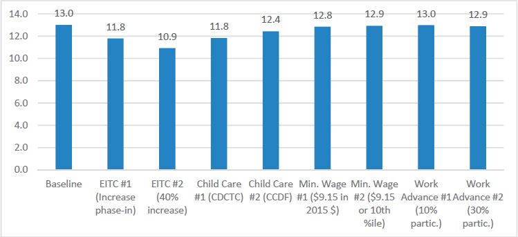
Summary-1) the greatest anti-poverty impact was achieved by a 40 percent increase in the EITC, which reduced child SPM poverty from 13.0 percent to 10.9 percent. A smaller increase in the EITC and an expansion of the CDCTC each reduced child poverty to 11.8 percent. Expansions to CCDF subsidies, reductions in the minimum wage, and the implementation of a WorkAdvance policy had smaller impacts.
Among policies expanding safety-net programs, the greatest antipoverty impact was achieved by an expansion to housing vouchers, in which 70 percent of eligible households with children currently lacking subsidies were assumed to obtain them. That policy reduced child poverty to 10.1 percent (see Figure Summary-2).
A third set of policies created universal benefits—child allowances and child support assurance programs. Of these, the policy with the greatest impact on child poverty was a $2,700-per-child child allowance, modeled using the existing CTC phase-out (see Figure Summary-3). The child support assurance policies that were modeled had smaller anti-poverty impacts than the child allowance policies.
Simulations of basic income guarantees (see Figure Summary-4) produced very large child poverty reductions. However, these policies were simulated without any modeling of employment or earnings impacts, so the results are not as directly comparable to the results of the other policies.
Finally, the Committee’s packages of policies reduced child SPM poverty to as low as 6.2 percent (see Figure Summary-5).
The model is also able to estimate the government costs of the policies, to the extent that the costs can be assessed at the household level. (The model does not capture administrative costs.) The costs of the policies were
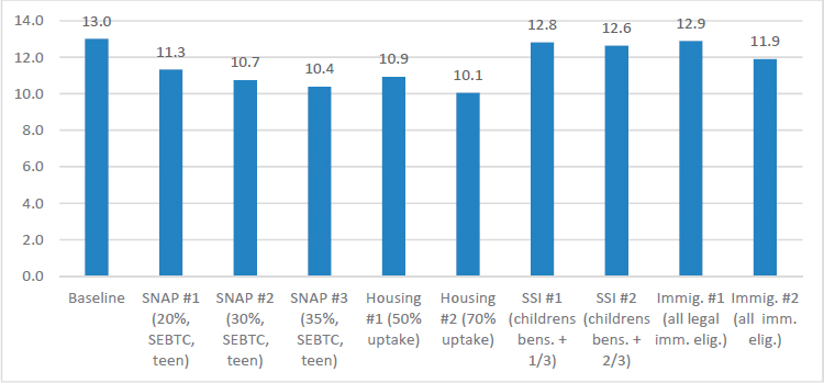
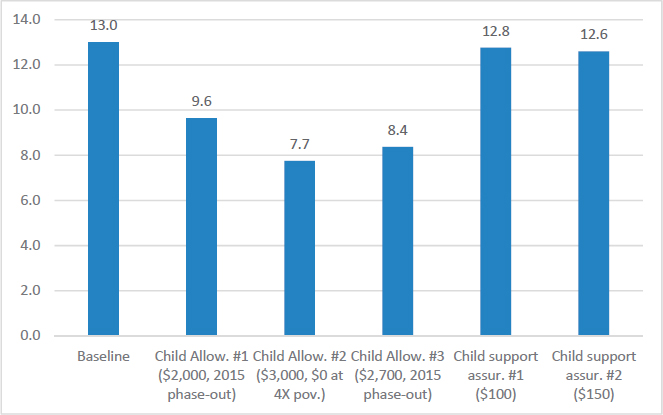
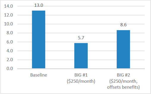
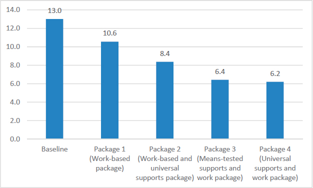
TABLE Summary-1 Percentage Point Reductions in Child Poverty and Government Costs, Selected Policies, Implemented in 2015
| Policy | Percentage Point Reduction in Child SPM Poverty | One-Year Government Cost, Millions |
|---|---|---|
| EITC #1 (Increase Phase-in) | 1.2 | 8,384 |
| EITC #2 (40% Increase) | 2.1 | 20,206 |
| Child Care #1 (CDCTC) | 1.2 | 5,141 |
| Child Care #2 (CCDF) | 0.6 | 6,894 |
| SNAP #1 (20%, SEBTC, Teen) | 1.7 | 26,414 |
| SNAP #2 (30%, SEBTC, Teen) | 2.3 | 37,390 |
| SNAP #3 (35%, SEBTC, Teen) | 2.6 | 43,075 |
| Housing #1 (50% Uptake) | 2.1 | 24,134 |
| Housing #2 (70% Uptake) | 3.0 | 34,916 |
| SSI #1 (Children’s Bens. + 1/3) | 0.2 | 4,235 |
| SSI #2 (Children’s Bens. + 2/3) | 0.4 | 9,386 |
| Immigration #1 (All Legal Imm. Elig.) | 0.1 | 3,933 |
| Immigration #2 (All Imm. Elig.) | 1.1 | 16,921 |
| Child Allow. #1 ($2,000, 2015 Phase-out) | 3.4 | 32,904 |
| Child Allow. #2 ($3,000, $0 at 4X Pov.) | 5.3 | 54,364 |
| Child Allow. #3 ($2,700, 2015 Phase-out) | 4.6 | 77,901 |
| Child Support Assurance. #1 ($100) | 0.2 | 5,660 |
| Child Support Assurance #2 ($150) | 0.4 | 8,843 |
NOTE: Does not include minimum wage policies (because cost is borne primarily by private sector, WorkAdvance (because a substantial portion of cost is administrative), or BIG (because employment effects were not modeled).
generally proportional to their anti-poverty impacts (see Table Summary-1 and Figure Summary-6). Considering the policies that alter benefit programs or taxes, plus the child allowance and child support assurance policies, the smallest reduction in child SPM poverty (0.1 percentage points) was produced by the policy to restore potential benefit eligibility to all legal immigrants, which had the lowest government cost ($3.9 billion) of any of the individual policies. At the opposite extreme, the individual policy with the largest anti-poverty impact—5.3 percentage points—had the second-largest cost, at $54.4 billion.
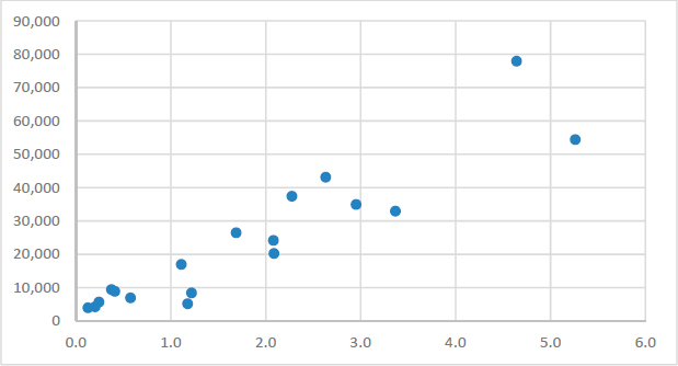
NOTE: The policies shown in this scatterplot are the same policies shown in Table Summary-1.
However, there are some cases in which a less-expensive policy has greater anti-poverty impact. For example, Child Allowance #1 reduces poverty by 3.4 percentage points but costs about $10 billion less than SNAP #3, which reduces child SPM poverty by 2.6 percentage points. Also, the child allowance policy with the greatest anti-poverty impact—child allowance #2—costs substantially less than child allowance #3, which had less anti-poverty impact.
Several caveats are important to note. First, the majority of the analysis is based on data representing the population, economy, and policies in 2015. Additional simulations tested the impacts of the policies when imposed on a modified baseline incorporating 2018 tax law, and showed that, in general, the relative impacts of the policies were similar. However, no attempt was made to adjust for difference in the population or the economy between 2015 and today.
Second, we do not incorporate into the model how the government would pay for any new or expanded programs. If new policies were funded by reducing spending on some current programs or by altering the tax system, the resources of low-income families could be impacted by those changes as well as by the new anti-poverty policies.
Third, the model focuses only on the immediate impacts of policy changes on children’s poverty. There is no estimation of how improvements in current economic well-being could affect children’s future education or employment outcomes.
Fourth, the cost estimates that are shown are the first-year costs of the policies, if they had been applied to the 2015 population with economic
circumstances as they were in 2015. Over a longer period, the annual costs would depend on changes in the total population, the economy, and the number and characteristics of people living in poverty.
Despite those limitations, the analysis shows the potential to substantially reduce child poverty through a combination of increased gains to work, increased safety net benefits, and new universal benefits. This report has summarized the methods used to create these estimates and presented overall results. Detailed programmatic results and substantial additional information on antipoverty impacts for demographic subgroups of children are available in appendix materials.
REFERENCES
Acs, G., Wheaton, L., Enchautegui, M., and Nichols, A. (2014). Understanding the Implications of Raising the Minimum Wage in the District of Columbia. Research report. Washington, DC: Urban Institute. Available: https://www.urban.org/research/publication/understanding-implications-raising-minimum-wage-district-columbia.
Allegretto, S. and Cooper, D. (2014). Twenty Three Years and Still Waiting for Change: Why it’s time to give tipped workers the regular minimum wage. Economic Policy Institute. Available: https://www.epi.org/files/2014/EPI-CWED-BP379.pdf.
Blau, D. (2003). Child care subsidy programs. In Means-Tested Transfer Programs in the United States, edited by Robert A. Moffitt. Chicago: University of Chicago Press. Available: http://www.nber.org/chapters/c10260.
Blau, F.D., and Kahn, L.M. (2007). Changes in the labor supply behavior of married women: 1980-2000. Journal of Labor Economics, 25(3), 393–438.
Blundell, R., and MaCurdy, T. (1999). Labor supply: A review of alternative approaches. Chapter 27 (pages 1559-1695) in Handbook of Labor Economics, edited by O.C. Ashenfelter and D. Card, Volume 3, Part A. London, UK: Elsevier.
Bollinger, C.R., Hirsch, B.T., Hokayem, C., and Ziliak, J.P. (Forthcoming). Trouble in the Tails? What We Know about Earnings Nonresponse Thirty Years after Lillard, Smith, and Welch. Journal of Political Economy. Available: https://www.journals.uchicago.edu/doi/pdfplus/10.1086/701807.
Children’s Defense Fund. (2015). Ending Poverty Now. Washington, DC. Available: http://www.childrensdefense.org/library/PovertyReport/EndingChildPovertyNow.html.
Cohen, E., Minton, S., Thompson, M., Crowe, E., and Giannarelli, L. (2016). Welfare Rules Databook: State TANF Policies as of July 2015. OPRE Report 2016-67. Washington, DC: Office of Planning, Research and Evaluation, Administration for Children and Families, U.S. Department of Health and Human Services.
Congressional Budget Office (CBO). (2017). June 2017 Baseline Forecast-Data Release (Calendar Year). Available: https://www.cbo.gov/sites/default/files/recurringdata/51135-201706-economicprojections2.xlsx.
Congressional Budget Office (CBO). (2014). The Effects of a Minimum Wage Increase on Employment and Family Income. Washington, DC. Available: https://www.cbo.gov/sites/default/files/113th-congress-2013-2014/reports/44995-MinimumWage_OneColumn.pdf.
Crouse, G., and Macartney, S. (2018). Welfare Indicators and Risk Factors. Seventeenth Report to Congress. Washington, DC: U.S. Department of Health and Human Services, Office of the Assistant Secretary for Planning and Evaluation. Available: https://aspe.hhs.gov/system/files/pdf/259196/WELFAREINDICATORS17THREPORT.pdf.
Cunnyngham, K. (2018). Reaching Those in Need: Estimates of State Supplemental Nutrition Assistance Program Participation Rates in 2015. Washington, DC: USDA Food and Nutrition Service. Available: https://fns-prod.azureedge.net/sites/default/files/ops/Reaching2015.pdf.
Eissa, N., and Hoynes, H. (2004). Taxes and the labor market participation of married couples: The Earned Income Tax Credit. Journal of Public Economics, 88, 1931–1958.
Food and Nutrition Service. (2016). State Options Report. Supplemental Nutrition Assistance Program. Options as of October 1, 2015. Washington, DC: United States Department of Agriculture. Available: https://fns-prod.azureedge.net/sites/default/files/snap/12-State_Options.pdf.
Fox, L. (2017). The Supplemental Poverty Measure: 2016. Current Population Reports P60261 (RV). Washington, DC: US Bureau of the Census. Available: https://www.census.gov/content/dam/Census/library/publications/2017/demo/p60-261.pdf.
Giannarelli, L., Lippold, K., Minton, S., and Wheaton, L. (2015). Reducing Child Poverty in the US: Costs and Impacts of Policies Proposed by the Children’s Defense Fund. Washington, DC: The Urban Institute. Available: https://www.urban.org/research/publication/reducing-child-poverty-us.
Giannarelli, L., Morton, J., and Wheaton, L. (2007). Estimating the Antipoverty Effects of Changes in Taxes and Benefits with the TRIM3 Microsimulation Model. Washington, DC: The Urban Institute. Available: http://www.urban.org/UploadedPDF/411450_Estimating_Effects.pdf.
Government Accountability Office. (2016). Supplemental Security Income. SSA Provides Benefits to Multiple Recipient Households but Needs System Changes to Improve Claims Management. GAO-16-674. Washington, DC. Available: https://www.gao.gov/assets/680/679137.pdf.
Gray, K.F., Fisher, S., and Lauffer, S. (2016). Characteristics of Supplemental Nutrition Assistance Program Households: Fiscal Year 2015. U.S. Department of Agriculture, Food and Nutrition Service, Office of Policy Support. Available: https://fns-prod.azureedge.net/sites/default/files/ops/Characteristics2015.pdf.
Hendra, R., Greenberg, D., Hamilton, G., Oppenheim, A., Pennington, A., Schaberg, K., and Tessler, B. (2016). Encouraging Evidence on a Sector-Focused Advancement Strategy. A Preview Summary of Two-Year Impacts from the Work Advance Demonstration. MDRC. Available: https://www.mdrc.org/publication/encouraging-evidence-sectorfocused-advancement-strategy.
Hoynes, H.W., and Patel, A.J. (2017). Effective policy for reducing poverty and inequality? The Earned Income Tax Credit and the distribution of income. Journal of Human Resources 53.
Hoynes, H.W., and Schanzenbach, D.W. (2012). Work incentives and the Food Stamp Program. Journal of Public Economics, 96, 151–162.
Jacob, B.A., and Ludwig, J. (2012). The effects of housing assistance on labor supply: Evidence from a voucher lottery. American Economic Review 102(1). Available: https://www.aeaweb.org/articles?id=10.1257/aer.102.1.272.
Lippold, K. (2015). Reducing Poverty in the United States: Results of a Microsimulation Analysis of the Community Advocates Public Policy Institute Policy Package. Project report. Washington, DC: Urban Institute. Available: https://www.urban.org/research/publication/reducing-poverty-united-states.
Mittag, N. (2016). Correcting for Misreporting of Government Benefits. IZA Discussion Paper No. 10266. Available: http://ftp.iza.org/dp10266.pdf.
Passel, J.S., and Clark, R. (1998). Immigrants in New York: Their Legal Status, Incomes, and Taxes. Project report. Washington, DC: The Urban Institute. Available: http://webarchive.urban.org/publications/407432.html.
Passel, J.S., and Cohn, D. (2011). Unauthorized Immigrant Population: National and State Trends 2010. Pew Research Hispanic Trends Project. Available: http://www.pewhispanic.org/2011/02/01/unauthorized-immigrant-population-brnational-and-state-trends-2010.
Passel, J.S., Van Hook, J., and Bean, F.D. (2006). Narrative Profile with Adjoining Tables of Unauthorized Migrants and Other Immigrants, Based on Census 2000: Characteristics and Methods. Warrington, PA: Sabre Systems, Inc.
Rothbaum, J. (2015). Comparing Income Aggregates: How do the CPS and ACS Match the National Income and Product Accounts? SEHSD Working Paper 2015-01. U.S. Bureau of the Census.
Stevens, K., Fox, L.E., and Heggeness, M.L. (2018). Precision in Measurement: Using State-Level SNAP Administrative Records and the Transfer Income Model (TRIM3) to Evaluate Poverty Measurement. SEHSD Working Paper No. 2018-15. U.S. Census Bureau. Available: https://www.census.gov/content/dam/Census/library/working-papers/2018/demo/SEHSD-WP2018-15.pdf.
Stevens, K., Minton, S., Blatt, L., and Giannarelli, L. (2016). The CCDF Policies Database Book of Tables: Key Cross-State Variations in CCDF Policies as of October 1, 2015. OPRE Report 2016-94. Washington, DC: Office of Planning, Research and Evaluation, Administration for Children and Families, U.S. Department of Health and Human Services.
Tessler, B.L., Bangser, M., Pennington, A., Schaberg, K., and Dalporto, H. 2014. Meeting the Needs of Workers and Employers. Implementation of a Sector-Focused Career Advancement Model for Low-Skilled Adults. MDRC. Available: https://www.mdrc.org/sites/default/files/CEO_WorkAdvanced_FR.pdf.
Trippe, C., Tadler, C., Johnson, P., Giannarelli, L., and Betson, D. (2018). National- and State-Level Estimates of WIC Eligibles and Program Reach in 2015. Project report to the Food and Nutrition Service. Available: https://www.fns.usda.gov/wic/national-and-state-levelestimates-special-supplemental-nutrition-program-women-infants-and-2.
Wheaton, L., and Stevens, K. (2016). The Effect of Different Tax Calculators on the Supplemental Poverty Measure. Research report. Washington, DC: Urban Institute. Available: https://www.census.gov/library/working-papers/2016/demo/wheaton-stevens-2016.html.
Zedlewski, S., Clark, S., Meier, E., and Watson, K. (1996). Potential Effects of Congressional Welfare Reform Legislation on Family Incomes. Washington DC: The Urban Institute.
Zedlewski, S., and Giannarelli, L. (2015). TRIM: A Tool for Social Policy Analysis. Washington, DC: Office of the Assistant Secretary for Planning and Evaluation, Department of Health and Human Services. Available: https://aspe.hhs.gov/pdf-report/trim-tool-social-policy-analysis.
ABOUT THE URBAN INSTITUTE
The nonprofit Urban Institute is dedicated to elevating the debate on social and economic policy. For nearly five decades, Urban Institute scholars have conducted research and offered evidence-based solutions that improve lives and strengthen communities across a rapidly urbanizing world. Their objective research helps expand opportunities for all, reduce hardship among the most vulnerable, and strengthen the effectiveness of the public sector.
Acknowledgments
This project was funded by the National Academy of Sciences, Division of Behavioral and Social Sciences and Education, Committee on Building an Agenda to Reduce the Number of Children Living in Poverty by Half in 10 Years. The views expressed are those of the authors and should not be attributed to the Urban Institute, its trustees, or its funders.
Information presented here is derived in part from the Transfer Income Model, Version 3 (TRIM3) and associated databases. TRIM3 requires users to input assumptions and/or interpretations about economic behavior and the rules governing federal programs. Therefore, the conclusions presented here are attributable only to the authors of this report.
The authors owe sincere thanks to Joyce Morton, Lead Programmer for TRIM3, whose expertise was critical for portions of this analysis. We also thank Ben Goehring, Christine Heffernan, and Victoria Tran for their assistance in simulating several of the policies and analyzing the results. In addition, we thank all the members of the TRIM3 project team whose work contributed to the development of the 2015 baseline simulations (which were the starting point for this project) or the maintenance of the technical aspects of the system during the project period. Those team members are: Elaine Maag and Sarah Minton (senior research staff); Lorraine Blatt, Elizabeth Crowe, Ben Goehring, Sweta Haldar, Christopher Hayes, Christine Heffernan, Caleb Quakenbush, Nathan Sick, Meg Thompson, and Victoria Tran (research staff); and Kara Harkins, Alyssa Harris, and Silke Taylor (programming staff).
We are grateful to the U.S. Department of Health and Human Services, Office of the Assistant Secretary for Planning and Evaluation (HHS/ASPE), for the ongoing support they provide to maintain the CPS-based TRIM3 model, and for granting permission for the HHS-funded TRIM3 baseline simulations to be used as the foundation for other analyses such as this one.
Urban Institute TRIM3 Project Consultants
Linda Giannarelli is a Senior Fellow in the Urban Institute’s Income and Benefits Policy Center, who has led or co-led the maintenance and development of TRIM3 for over 20 years. Her research focuses on the interactions across safety net programs and the use of microsimulation to assess the potential impacts of policy changes on the economic well-being of lower-income families.
Laura Wheaton is a Senior Fellow in the Urban Institute’s Income and Benefits Policy Center, specializing in analyzing government safety net programs, poverty estimation, and the microsimulation modeling of tax and transfer programs. Wheaton co-directs the TRIM3 microsimulation model
project. Her recent projects include an analysis of the anti-poverty effects of nutrition assistance programs.
Joyce Morton is a Senior Research Associate in the Urban Institute’s Income and Benefits Policy Center and Lead Programmer/Analyst for the TRIM3 and ATTIS simulation models. She has worked for more than 20 years with policy analysts and technical staff to develop the simulation models used to assess the impact of changes to safety net programs.
Kevin Werner is a Research Analyst in the Urban Institute’s Income and Benefits Policy Center. He focuses on the development and application of TRIM3 to analyze public assistance programs. He holds a master’s degree in Applied Economics from Georgetown University.


