
Appendix D
Cobweb Model of the Engineering Labor Market
In any occupation, the higher the wage, the more people are willing to work in it, so the supply curve is upward sloping. On the other hand, the higher the wage, the fewer workers employers are willing to hire, so the demand curve is downward sloping.
The supply of workers comprises US citizens, permanent residents, and those with temporary visas (such as the H-1B) who have engineering skills and knowledge that can be used in engineering and other occupations.
Wage and employment levels are determined by the intersection of the demand and supply curves. When there are shifts in demand or supply, known as shocks, the market adjusts. The seminal work of Freeman (1976) used data on degreed engineers to establish a “cobweb” model for the adjustments of the labor market (also see Ryoo and Rosen 2004).
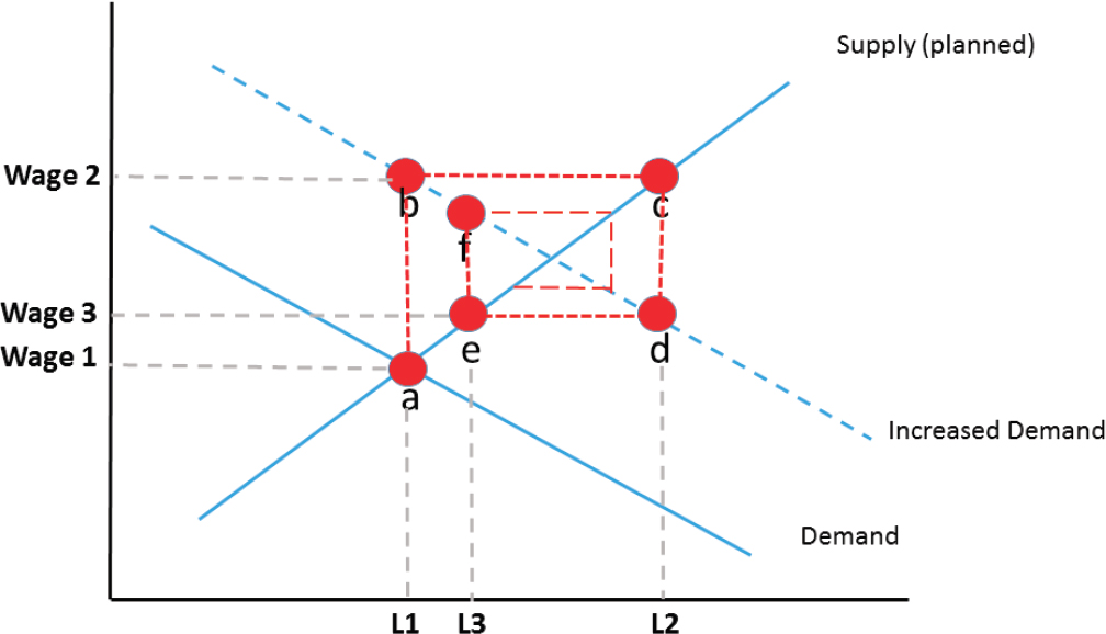
To understand the “cobweb” model, consider the labor market for engineers as sketched in figure D-1, initially in equilibrium (point a) at the intersection of long-run Supply and Demand, with L1 engineers employed at Wage 1. An increase in demand for engineers, such as the establishment of NASA in 1958 (Freeman 1976), shifts demand out to Increased Demand, and the long-run equilibrium lies at the intersection of Increased Demand and Supply.
However, if demand increases suddenly, there is no time for new engineers to be trained (although some might delay retirement or return early from parental leave), and the market equalizes supply and demand through a jump up in wages to W2. In other words, while the long-run supply curve is as drawn in blue, the very short-run supply curve is vertical at L1 (red dotted line).
For about four years (if supply is dependent on new US graduates entering the market, not a surge in engineers from offshore), the market is likely to stay at point b, with employers complaining of “shortages” (i.e., high wages). Meanwhile, the higher wage induces more students to study engineering: the number of people willing to work as engineers when the wage is Wage2 is given by the long-run supply curve (point c): after four years, there will be L2 engineers. Once the additional engineers enter the market, however, the wage drops: with a greater number of engineers from which to choose, employers are now willing to hire L2 engineers only at wage Wage3 (point d).
With the drop in wages, there is likely to be talk of a “glut” of engineers four years after complaints of “shortages.” Enrollment in engineering declines (and some adjustment occurs through withdrawals from the labor force), and four years later engineering employment is at L3. As the long-run equilibrium has not yet been achieved, there is likely to be another set of cycles, as in points e and f, which illustrate why the process is called a cobweb cycle.
The more forward-looking students are, and the more there can be adjustment without lengthy training, the faster the equilibrium will be achieved. Since the expansion in 1990 of the number of skilled immigrant temporary
Source: Adapted with permission from https://policonomics.com/cobweb-model.
visas permitted, immigration has allowed just such a short cut to the equilibrium. The number of engineers can be changed with no more than a year’s lag (the time to apply for the annual visa distribution), so the long-run supply curve is flatter: the cycles are both faster and associated with smaller wage changes.
REFERENCES
Freeman RB. 1976. A cobweb model of the supply and starting salary of new engineers. Industrial and Labor Relations Review 29(2):236–248.
Ryoo J, Rosen S. 2004 The engineering labor market. Journal of Political Economy 112 (February):S110–S140.


