
3
Using Genes and Genomes to Identify Species and Subspecies
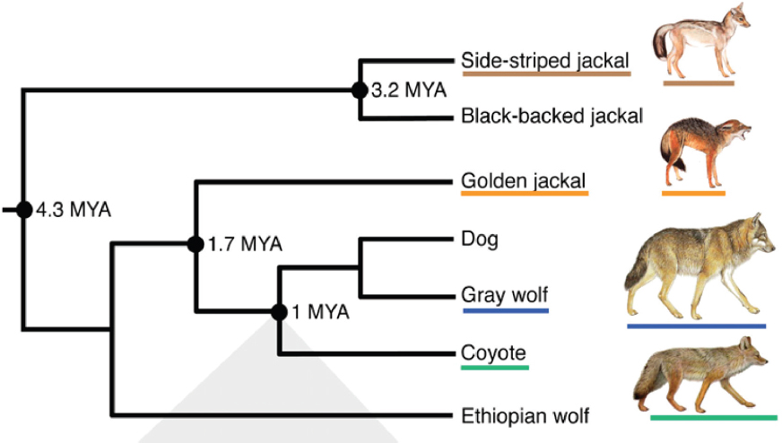
Genetic techniques have become increasingly sophisticated and complicated over the past few decades. The advances in genetic techniques enable scientists to describe the entire genome of an organism and provide the computational power to compare genomes among many organisms. In contrast to the time when George Gaylord Simpson made the assessment quoted above, genetic analyses can now provide this “most priceless data” for reconstructing the phylogenies of species (Figure 3-1).
The nuclear DNA of canids consists of a haploid genome of approximately 2.5 billion base pairs. Thus, the nucleus of each cell contains two copies of this haploid genome, one maternally derived and the other paternally derived. In addition to the nuclear DNA, the mitochondrial genome of a cell contains its own haploid genome of approximately 16,000 base pairs of DNA (mtDNA), which are usually passed on from mother to offspring. Differences in the DNA sequences of individuals, within and between species, arise as a consequence of mutations of various types—those that replace one base pair with another, those that delete or insert new base pairs, and those that re-arrange the order of the base pairs. Description of such genetic changes can provide insight into the past history, as well as into the current reproductive relationships, of populations and species.
This chapter presents an introduction to fundamental concepts and methods necessary to understand the available genetic papers discussed in Chapters 4 and 5, and the committee’s answer to the taxonomic questions in the statement of task. The first topic is the use of single genes to detect genetic differences between individuals and populations within species as well as genetic differences between species. This is followed by explanations of the use of mtDNA to reconstruct the
phylogeny of populations and species and of the use of whole-genome sequence data to describe genetic similarity, phylogeny, and taxonomic relationships among populations and species.
INDIVIDUAL NUCLEAR GENES
Early studies of genetic variation in wolves relied on comparing the DNA sequence at individual locations (loci) within the genome. Different sequences at the same locus are called alleles. The early studies of genetic variation in wolves found such allelic differences at many loci throughout the genome.
Microsatellites
Microsatellites are repetitive segments of DNA that are widely distributed throughout the genome. Microsatellite loci often have many alleles because they have exceptionally high mutation rates (Schlötterer, 1998). The presence of many alleles in populations make these loci especially valuable for estimating genetic differences between individuals and between populations. Hedrick et al. (1997) compared allele frequencies at 20 microsatellite loci in Mexican gray wolves with those found in domestic dogs, northern gray wolves, and coyotes to determine whether the Mexican wolves had unique alleles (two of these loci are shown in Table 3-1). For example, the I allele at the 172 locus was at a frequency of 0.944 in dogs (i.e., 94.4 percent of the alleles genotyped at this locus in dogs were I), but the frequency of the I allele in Mexican gray wolves was only 0.050. In contrast, the G and H alleles were at a combined frequency of 0.950 in Mexican gray wolves, but these alleles were not present in dogs. The researchers concluded on the basis of all 20 loci that the three captive populations of Mexican gray wolves were closely related to each other and they were distinct from dogs and northern gray wolves.
TABLE 3-1 Allele Frequencies at Two Representative Microsatellite Loci (172 and 204) in Gray Wolves, Coyotes, and 27 Breeds of Dogs
| Locus 172 | Locus 204 | ||||||
|---|---|---|---|---|---|---|---|
| G | H | I | A | B | D | E | |
| Mexican gray wolf | 0.825 | 0.125 | 0.050 | 0.211 | 0.158 | 0.500 | 0.132 |
| Northern gray wolf | 0.076 | 0.467 | 0.413 | 0.300 | 0.067 | 0.467 | 0.144 |
| Coyote | 0 | 0.320 | 0.160 | 0.909 | 0.091 | 0 | 0 |
| Dog | 0 | 0 | 0.944 | 0.396 | 0.021 | 0.021 | 0 |
NOTE: The allele frequencies do not sum to 1.0 in all cases because alleles not present in Mexican gray wolves are not shown.
SOURCE: Hedrick et al., 1997.
Single Nucleotide Polymorphisms (SNPs)
Researchers’ ability today to sequence entire genomes allows them to detect genetic differences at many positions throughout the genome. There are some 2.5 billion base pairs in the wolf haploid genome. It is now possible to compare nucleotide differences (A, T, G, or C) at hundreds of thousands of points in the genome where the individual base pairs vary; these points in the genome are referred to as single nucleotide polymorphisms, or SNPs. For example, Fitak et al. (2018) genotyped Mexican gray wolves, northern gray wolves, and domestic dogs at more than 172,000 SNPs. They found that Mexican gray wolves are highly distinct from northern gray wolves and that they lack any detectable admixture from dogs.
MITOCHONDRIAL DNA
The DNA in the mitochondria of mammals is usually transmitted to offspring from their mother. All of the copies of this sequence within a given individual are identical (a situation referred to as haploid). This differs from the situation for nuclear DNA, where each individual has two copies, one from each parent (or diploid). There is no recombination1 in haploid mtDNA, as there is in nuclear DNA. Therefore, mtDNA is inherited as a single locus. Any single locus by itself is not very useful for describing genetic population structure, as noted in the previous section, because the patterns of differentiation between loci will differ by chance alone. Therefore, describing the amount of genetic differentiation between populations or species requires comparing the patterns of differentiation at many loci (e.g., the 20 nuclear loci examined in Hedrick et al., 1997).
On the other hand, the lack of recombination between mtDNA molecules makes them an especially useful marker for reconstructing phylogenetic history. Phylogenetic trees depict the evolutionary history of the relationships among species (Figure 3-1). Species that are more closely related evolutionarily share a more recent common ancestor than more distantly related species, and they appear closer together in a phylogenetic tree. It is important to keep in mind, however, that phylogenies based upon mtDNA reflect only matrilineal genealogical relationships among individuals because only females pass their mtDNA on to offspring.
A gene tree (such as one constructed on the basis of mtDNA) is a phylogenetic tree constructed from a particular gene from each of the species under study. A phylogenetic tree based upon any
___________________
1 Also referred to as genetic reshuffling, recombination is the exchange of DNA between parental chromosomes during the formation of sperm and egg. The result of this exchange is the production of offspring with a combination of genes that differs from either parent.
single gene (a gene tree) may or may not be concordant with the actual phylogenetic history of the species under consideration (species tree).
Most new mutations are lost by chance (genetic drift) before they become common within a population. However, some new mutations increase in frequency in the population due to genetic drift or because of the directional forces of natural selection. When a mutation reaches a frequency of 1.0 in the population—i.e., it has become “fixed”—we say that a substitution has occurred. Most of the time, the mutations that are used in genetic comparison of species are mutations that replace one base with another. The longer that two species are isolated from each other, the more such substitutions they will demonstrate.
The presence or absence of fixed differences does not always provide unambiguous insight into questions regarding species or subspecies status. In some cases, different species may share polymorphisms.2 This can occur two ways. First, the species may have diverged recently from each other. In this case, insufficient time has elapsed for different alleles to be fixed in the species. This pattern is denoted as “incomplete lineage sorting.” Second, there may have been introgression which introduced alleles from one species into another. In either case, the gene trees constructed from these genes may not match the actual phylogenetic history of the two species. A method for distinguishing these two causes of shared polymorphisms, the so-called ABBA/BABA analysis, is discussed below.
The earliest attempts to use molecular data to construct the phylogenetic trees of wolves were based on mtDNA sequences. For example, in Vilà et al. (1999), researchers compared the sequences of 350 base pairs of mtDNA from a worldwide sample of gray wolves and coyotes. The researchers found that more sequence variability was found in coyotes than in wolves. Thirty-four different mtDNA sequences (haplotypes) were found in 259 wolves, while 15 different mtDNA haplotypes were found in just 17 coyotes. On average, the 34 gray wolf haplotypes differed from each other by 5.3 substitutions. The 15 coyote haplotypes differed from each other by an average of 7.4 substitutions. And the gray wolf haplotypes differed from coyote haplotype by an average of 18.8 substitutions.
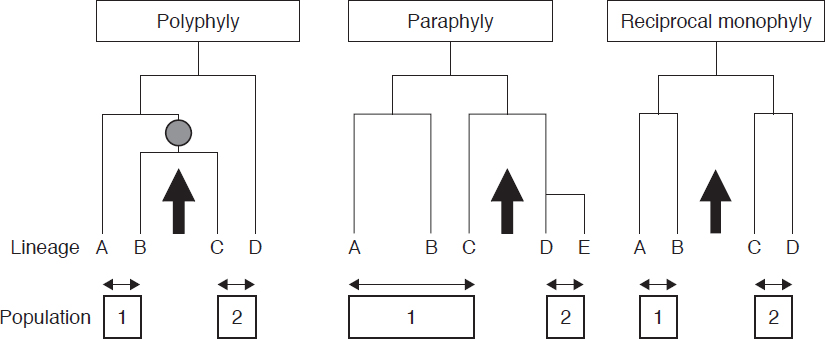
For many species, every individual within the species shares a more recent common ancestor that is not shared with any individuals in other species, a situation known as monophyly (Figure 3-2). The mtDNA sequences reported by Vilà et al. (1999) are reciprocally monophyletic. That is, all of the gray wolf haplotypes share a more recent common ancestor with each other than any of them do with the coyote haplotypes.
Recently diverged species can be non-monophyletic, that is, there may be individuals in one population who share a more recent common ancestor with individuals in the other population than they do with some individuals in their own population. The resulting situation can be either polyphyly or paraphyly, depending on the details of the phylogenetic relationships between the members of the different populations (Figure 3-2). Also, as discussed in Chapter 2, the introgression of mitochondria from one species to another can result in a lack of reciprocal monophyly for mtDNA (in which case the molecular genealogies of mtDNA overlap). For this reason, phylogenies estimated from any single genetic marker, such as mtDNA, might not necessarily reflect the true historical relationships among the populations or species represented by the individuals included in the analysis.
GENOMES
Most recent studies with wolves have described sequence differences over the entire 2.5 billion base pair wolf haploid genome in order to describe the genetic relationships among different
___________________
2 The presence of two or more alleles at the same gene locus within a population.
groups. However, population genomics is more than simply using more loci (e.g., 172,000 SNPs versus 20 microsatellite loci). Population genomics requires having a linkage map showing the chromosomal locations and rates of recombination between different loci so that particular regions of the genome can be studied (e.g., regions of the genome inherited from one of the two contributing parental populations in admixed individuals). That is, instead of using a representative sample of loci to address the average effect of processes acting across the whole genome, population genomics describes variation in those processes in specific regions of the genome.
For example, Sinding et al. (2018) used 40 full-genome sequences to describe the genetics and evolutionary relationships among extant wolves and wolf-like canids in North America. The authors conclude that all North American gray wolves, including the Mexican gray wolf, are monophyletic and thus share a common ancestor that is not shared with any other wolves. They also concluded that the red, Eastern timber, and Great Lakes wolves demonstrate admixture between modern gray wolves and coyotes. Although there were population-specific sequences in their samples of these taxa that might distinguish them from gray wolves and coyotes, the authors did not have sufficient samples to draw conclusions about the significance of these sequences.
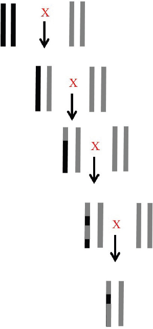
Nuclear DNA differs from mtDNA in many ways, the most important of which are biparental inheritance and the process of recombination. Figure 3-3 illustrates the effects of recombination following the production of hybrids that are then continually crossed back to one of the parental species.
Another difference is that mtDNA has a much higher mutation rate than nuclear DNA; this results in a greater rate of substitution per generation for mitochondrial DNA than for nuclear DNA. Different regions of the nuclear genome will have different gene trees (phylogenies) because of recombination. As mentioned in the discussion of mtDNA trees, some of these trees may differ from
the true species trees because of shared ancestral variation. A phylogeny estimated from nuclear DNA will then reflect a genomic average among all of the trees, but it might not be representative of any specific region of the genome. This problem is not as much of a concern in very distantly related species because the chance of them harboring shared ancestral variation is much less. In addition, because of the enormous size of the nuclear genome, nuclear DNA provides a very large number of independent observations for use in statistical analyses of hypotheses regarding population histories.
Model-Based Approaches
The timing and directionality of an admixture between populations and species can be estimated using model-based approaches. These approaches make various assumptions about the underlying population genetic model in order to estimate the parameters of interest (e.g., migration rates, divergence times between populations, etc.). The model in the software package G-PhoCS (for Generalized Phylogenetic Coalescence Sampler) can be used to calculate posterior probabilities
for species tree topologies, migration rates, and divergence times, using genomic data, with the assumption that the input is from multiple independent non-recombining loci (Gronau et al., 2011). Using this program, vonHoldt et al. (2016) estimated that red wolves evolved as a sister group to coyotes 55,000–117,000 years ago, depending on the model’s assumptions. One important thing to keep in mind regarding many of the methods like this is that they rely on very strong model assumptions, for example, regarding the history of population size changes. Furthermore, they require a tremendous amount of computing power to carry out the calculations, which can lead to various computational problems including, in some cases, providing unstable results.
Genetic Similarity
Some methods of analyzing genomic data look at the genetic similarity of individuals but do not attempt to reconstruct phylogenies in the way discussed above. The more recently that two species shared a common ancestor, the more likely they are to be genetically similar. Therefore, comparing the genetic similarity of individuals can also provide insight about evolutionary relationships. However, certain population genetic processes can obscure these relationships. For example, genetic drift resulting from a small population bottleneck can result in the individuals within a population being very similar to each other and very distinct from even closely related populations.
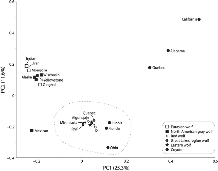
One common type of analysis of genomic data is principal component analysis (PCA) (e.g., Novembre and Stephens, 2008). Principal component analysis, a statistical procedure that simplifies a set of observations on many variables into just a few underlying variables called principal components (PC), is based on genetic similarity. Principal components are uncorrelated with each other, and they can be used to display the total variation in the observations along uncorrelated axes of variation (e.g., PC1). This allows for the identification of clusters of genetically similar individuals. For example, Figure 3-4 shows a PCA of 5.4 million SNPs in 23 Canis genomes. The first axis (PC1) explains 25.3 percent of the total variability in the data, and PC2 explains 11.6 percent of the total variation.
Clusters of genetically similar individuals may occur because the individuals grouped together form a species, subspecies, or population. However, individuals might also cluster together if they are similarly admixed between other species, even if they otherwise share little common history. Also, the axis of variation identified by PCA is strongly dependent on sample size because small sample sizes may fail to capture phenotypes that are comparatively rare. As such, PCA does not provide definitive evidence regarding species or subspecies status (Figure 3-4).
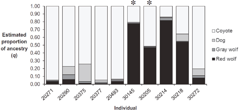
The software program STRUCTURE (Pritchard et al., 2000) categorizes individuals as belonging fractionally to one or more populations on the basis of fundamental population-genetic principles (e.g., genotypic proportions expected with random mating). STRUCTURE analysis can be also used to identify admixture components (Figure 3-5). The admixture components identified with STRUCTURE are typically interpreted as being representative of ancestral populations that may have existed at some (unspecified) time in the past before the admixture happened. In most analyses, the number of admixture components (k) is considered fixed, but there are also methods that attempt to estimate the value of k. When individuals are assigned to the same admixture component, this provides evidence that they have similar alleles. This might be because they have been isolated from other individuals for a long time, or it could, for example, be because they both descended from a population that very recently experienced a sharp reduction in its size. Therefore, admixture analysis using STRUCTURE does not necessarily reflect the hierarchical evolutionary structure of the sample. Also, as is the case with PCA, the sample sizes have significant effects in determining which components are identified.
Ancestry Painting of Chromosomes
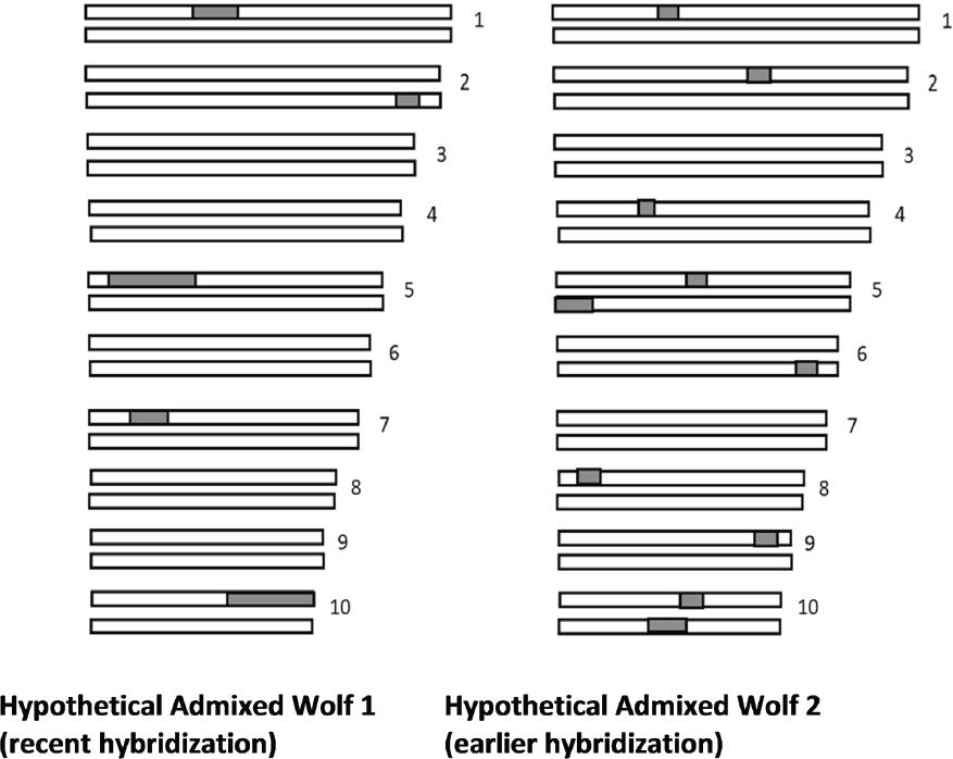
Statistical methods similar to STRUCTURE analysis can be used to identify particular segments of the genome that originate from various pre-defined reference species in admixed populations (Maples et al., 2013). In one method, called ancestry painting of chromosomes, different regions of the chromosomes are color-coded to reflect from which of pre-defined reference species they originated (Figure 3-6). Different individuals in the same population can have different amounts of admixture. In addition, the length of the admixture segments provides information about the amount of time since the hybridization event.
Ancestry painting is a very powerful tool both for detecting hybridization and estimating the time since hybridization. However, its reliability depends heavily on using the appropriate reference populations, and it may produce erroneous results if inappropriate reference populations are used. For example, one could analyze dog chromosomes as an admixture between a mouse and horse,
and this would result in the identification of some segments of the dog genome that look either horse- or mouse-like. However, this would clearly not imply that the dog is an admixture between a horse and a mouse. Thus, ancestry painting is not an appropriate or useful tool to determine the presence or absence of admixture if the correct reference populations are not used.
Detection of Admixture with ABBA/BABA
There are many whole-genome methods available to detect and estimate the amount of admixture (see Sinding et al., 2018). One powerful statistical tool for identifying admixture is the so-called ABBA/BABA analyses (Green et al., 2010), which use the genome-wide average of shared mutations to determine whether there is evidence for admixture. This is achieved by comparing the amount of shared mutations with a possibly admixed population to the amount of shared mutations with a population that is hypothesized not to be admixed (or at least contains less admixture). The test considers ancestral (A) and derived (B) alleles and is based on the prediction that two particular patterns of SNPs, termed ABBA and BABA, should be equally frequent under a scenario of incomplete lineage sorting without gene flow. An excess of ABBA or BABA patterns relative to the other is indicative of gene flow between two of the taxa. For example, the introgression of Neanderthals into modern humans was identified by noting that people outside of Africa share more substitutions with Neanderthals than do individuals inside Africa, a place where Neanderthals are thought never to have been present. While the ABBA/BABA analysis is very powerful for identifying admixture, it does not say anything about the directionality and timing of the admixture. We discuss in Chapter 5 how vonHoldt et al. (2016) used this approach to test the phylogenetic hypothesis of a sister taxa relationship between red wolf and coyote.
REFERENCES
Allendorf, F. W., G. Luikart, and S. N. Aitken. 2013. Genetics and the Conservation of Populations, 2nd ed. Oxford, UK: Wiley-Blackwell Publishing.
Bohling, J. H., and L. P. Waits. 2015. Factors influencing red wolf–coyote hybridization in eastern North Carolina, USA. Biological Conservation 184:108-116.
Fitak, R. R., S. E. Rinkevich, and M. Culver. 2018. Genome-wide analysis of SNPs is consistent with no domestic dog ancestry in the endangered Mexican wolf (Canis lupus baileyi). Journal of Heredity 109(4):372-383.
Green, R. E., J. Krause, A. W. Briggs, T. Maricic, U. Stenzel, M. Kircher, N. Patterson, H. Li, W. Zhai, M. H.-Y. Fritz, N. F. Hansen, E. Y. Durand, A.-S. Malaspinas, J. D. Jensen, T. Marques-Bonet, C. Alkan, K. Prüfer, M. Meyer, Hernán A. Burbano, J. M. Good, R. Schultz, A. Aximu-Petri, A. Butthof, B. Höber, B. Höffner, M. Siegemund, A. Weihmann, C. Nusbaum, E. S. Lander, C. Russ, N. Novod, J. Affourtit, M. Egholm, C. Verna, P. Rudan, D. Brajkovic, Ž. Kucan, I. Gušic, V. B. Doronichev, L. V. Golovanova, C. Lalueza-Fox, M. de la Rasilla, J. Fortea, A. Rosas, R. W. Schmitz, P. L. F. Johnson, E. E. Eichler, D. Falush, E. Birney, J. C. Mullikin, M. Slatkin, R. Nielsen, J. Kelso, M. Lachmann, D. Reich, and S. Pääbo. 2010. A draft sequence of the Neandertal genome. Science 328:710-722.
Gronau, I., M. J. Hubisz, B. Gulko, C. G. Danko, and A. Siepel. 2011. Bayesian inference of ancient human demography from individual genome sequences. Nature Genetics 43:1031-1034.
Hedrick, P. W., P. S. Miller, E. Geffen, and R. Wayne. 1997. Genetic evaluation of the three captive Mexican wolf lineages. Zoo Biology 16:47-69.
Maples, B. K., S. Gravel, E. E. Kenny, and C. D. Bustamante. 2013. RFMix: A discriminative modeling approach for rapid and robust local-ancestry inference. American Journal of Human Genetics 93:278-288.
Novembre, J., and M. Stephens. 2008. Interpreting principal component analyses of spatial population genetic variation. Nature Genetics 40:646-649.
Pritchard, J. K., M. Stephens, and P. Donnelly. 2000. Inference of population structure using multilocus genotype data. Genetics 155:945-959.
Schlötterer, C. 1998. Microsatellites. Pp. 237-262 in Molecular Genetic Analysis of Populations, A. R. Hoelzel, ed. New York: Oxford University Press.
Simpson, G. G. 1945. The principles of classification and a classification of mammals. Bulletin of the American Museum of Natural History 85:1-350.
Sinding, M.-H. S., S. Gopalakrishan, F. G. Vieira, J. A. Samaniego Castruita, K. Raundrup, M. P. Heide Jørgensen, M. Meldgaard, B. Petersen, T. Sicheritz-Ponten, J. B. Mikkelsen, U. Marquard-Petersen, R. Dietz, C. Sonne, L. Dalén, L. Bachmann, Ø. Wiig, A. J. Hansen, and M. T. P. Gilbert. 2018. Population genomics of grey wolves and wolf-like canids in North America. PLOS Genetics 14:e1007745.
Vilà, C., I. R. Amorim, J. A. Leonard, D. Posada, J. Castroviejo, F. Petruccifonseca, K. A. Crandall, H. Ellegren, and R. K. Wayne. 1999. Mitochondrial DNA phylogeography and population history of the grey wolf Canis lupus. Molecular Ecology 8:2089-2103.
vonHoldt, B. M., J. A. Cahill, Z. Fan, I. Gronau, J. Robinson, J. P. Pollinger, B. Shapiro, J. Wall, and R. K. Wayne. 2016. Whole-genome sequence analysis shows that two endemic species of North American wolf are admixtures of the coyote and gray wolf. Science Advances 2(7):e1501714.
vonHoldt, B. M., J. P. Pollinger, D. A. Earl, J. C. Knowles, A. R. Boyko, and H. Parker. 2011. A genome-wide perspective on the evolutionary history of enigmatic wolf-like canids. Genome Research 21:1294-1305.
This page intentionally left blank.


