
Chapter 2: Committee’s Review of the Study
This chapter provides comments on the overall Study, including an issue that cuts across all of the Study chapters. Subsequent sections of this chapter also provide more detailed reviews of each Study chapter. A chapter-by-chapter summary makes particular sense in this case as the Study chapters cover specific tasks involved in air quality modeling and the analysis and development of the EET methods. The committee’s assessment of how the Study accomplishes each objective is detailed in the individual chapter reviews (see Table 1.1 for the mapping of each objective).
COMMENTS ON THE OVERALL STUDY
The committee commends the authors for the extensive amount of work that was done to conduct the Study. The amount of meteorological (Weather Research and Forecasting [WRF]), emissions (National Emissions Inventory [NEI], detailed analysis for the Gulf of Mexico Region [GOMR]), and air quality modeling (Comprehensive Air Quality Model with Extensions [CAMx], American Meteorological Society/Environmental Protection Agency Regulatory Model [AERMOD], Offshore and Coastal Dispersion [OCD], CALPUFF) is significant. The Study: (a) evaluates the base case performance and tests a number of emissions scenarios using photochemical modeling; (b) applies, evaluates, and compares multiple dispersion models; and (c) develops and tests a number of emission exemption thresholds (EETs), including a new approach using Classification And Regression Tree (CART) analysis.
In particular, the Study provides a detailed accounting of emissions in the GOMR. This involved developing an inventory for sources in the Gulf of Mexico including those that are specific to oil and gas exploration, development, and production. The Study also needed an inventory of emissions in Mexico, both at the 4-km level for part of the Gulf Coast that is included in the 4-km modeling domain and at the 12- and 36-km levels. All of this work appears to have been done carefully and with attention to detail, and the Study authors deserve credit for this effort.
Overall, the Study addresses each of the objectives, although to varying degrees of accuracy and completeness (see individual Study chapter reviews for more detail). The findings are documented credibly, though in some cases in a rather abbreviated fashion, and are overly reliant on the information in the appendices. At times, the findings and their support are obscure (e.g., the comparison of dispersion models). The committee also noted that there is no Appendix A; the appendices start with Appendix B.1.
In general, the Study authors did reference the scientific literature, though greater reflection of the scientific literature is called for. For example, several published studies that have evaluated the emissions inventories used in the Study are not cited or used to assess the uncertainties in the modeling. Some of the references and analysis should consider more recent literature. This in part reflects the length of time from when the Study originated. Critical content areas that are missing are detailed in the chapter reviews below.
The text often uses subjective terms when a more quantitative or neutral description is suggested (e.g., the use of terms like “well” and “good”), unless there is support for such terms being used.
In Chapter 3 of the Study, the presentation of the modeled emissions and the lack of quantitative detail make it difficult to judge the credibility of the new inventory. Another term that the Study uses is “validate” when referring to the various models. As noted by Oreskes (1998), environmental models cannot be validated (or verified). The Study authors should review that paper and the NRC (2007) report Models in Environmental Regulatory Decision Making as to how to report the Study findings and to formulate future studies, with particular focus on model evaluation and quantifying and communicating uncertainties.
Implications of the Choice for the Base Case Year
A specific issue that cuts across all chapters is the choice of 2012 as a base case year for much of the analyses. The modeling analysis has two primary objectives: (1) to assess the emissions impact of the 5-year lease sales, and (2) for EET development.
The Study argues that the modeling should be performed for 2012, as the summer of 2011 was an exceptional year in terms of temperature and precipitation, and 2012 was a more average year in terms of meteorological conditions. However, choosing an average year in the 1918-2012 record likely underestimates the temperatures that are expected in the future during pollution episodes.
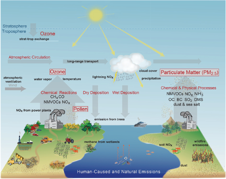
Climate change-driven changes in weather-related processes will impact future air quality. Air quality is driven by several weather conditions, such as temperature, wind patterns, cloud cover, and precipitation (Nolte et al., 2018; see Figure 2.1). For example, hot, sunny (higher photolysis), stagnant (less dispersion) days can increase ozone levels. Temperature is often the largest single driver for ozone (Jacob and Winner, 2009; Shen et al., 2017). Furthermore, higher temperatures themselves lead to increased evaporative and different biogenic volatile organic compounds (VOC) emissions, which are ozone precursors (e.g., Jacob and Winner, 2009; Rubin et al., 2006), as well as more rapid chemistry and organonitrate decomposition.
According to the National Climate Assessment, the U.S. annual average temperature has increased by 1.8°F (1°C) since the early 1900s and it is expected that it will increase an additional 2.5°F over the next few decades, regardless of future emissions (Hayhoe et al., 2018). Moreover, recent record-setting hot years are projected to become common in the near future (Vose et al., 2017). Such warming trends are also projected for all Gulf States in different emissions scenarios (representative concentration pathway [RCP] 4.5 and RCP8.5; Hayhoe et al., 2018).
The summer of 2011 in Texas was not only exceptional in terms of temperature, but also in precipitation. Rainfall can greatly affect the removal of air pollutants from the atmosphere. The year 2012 was a regular year with typical rainfall amount in the Southeastern United States. As it is projected that climate in this region is going to be generally drier (Hayhoe et al., 2018), using 2012 as the year for meteorology inputs would lead to more removal due to wet deposition, thus leading to lower estimation of the outer continental shelf (OCS) impact on onshore receptors.
Thus, choosing a different meteorological modeling year that had conditions most conducive to ozone formation may provide a different picture of how the OCS emissions contribute to ozone nonattainment and visibility impairment (see Figure 2.2).
It should be noted that drought conditions may affect biogenic emissions from different regions in complex ways. Ying et al. (2015) modeled biogenic emissions under drought conditions in
Texas in 2011 and analyzed the corresponding changes in ozone. Their study concludes that the impact on ozone due to drought related biogenic emission change is likely small in most areas and has little impact on the overall model performance of ozone. The driving force that caused the differences in biogenic emissions between 2011 and 2012 is the temperature difference. The uncertainty in modeling the emissions under drought condition should not prevent the Study authors from considering 2011 as the base year for the Study.
The choice of 2012 as the base year also propagates into the modeling of the future year (2036), as the meteorological fields are kept the same. As a result, emissions of biogenic VOCs from vegetation and emissions from wildfires are the same between the base year and the future year (Figure 4-3 of the Study). Accounting for predicted changes in climatological conditions would have led to different biogenic and wildfire emissions and potentially higher impacts from the new oxides of nitrogen (NOX) emissions offshore.
___________________
1 Text modified January 2020. Throughout the report, PM10 was added where PM2.5 is mentioned.
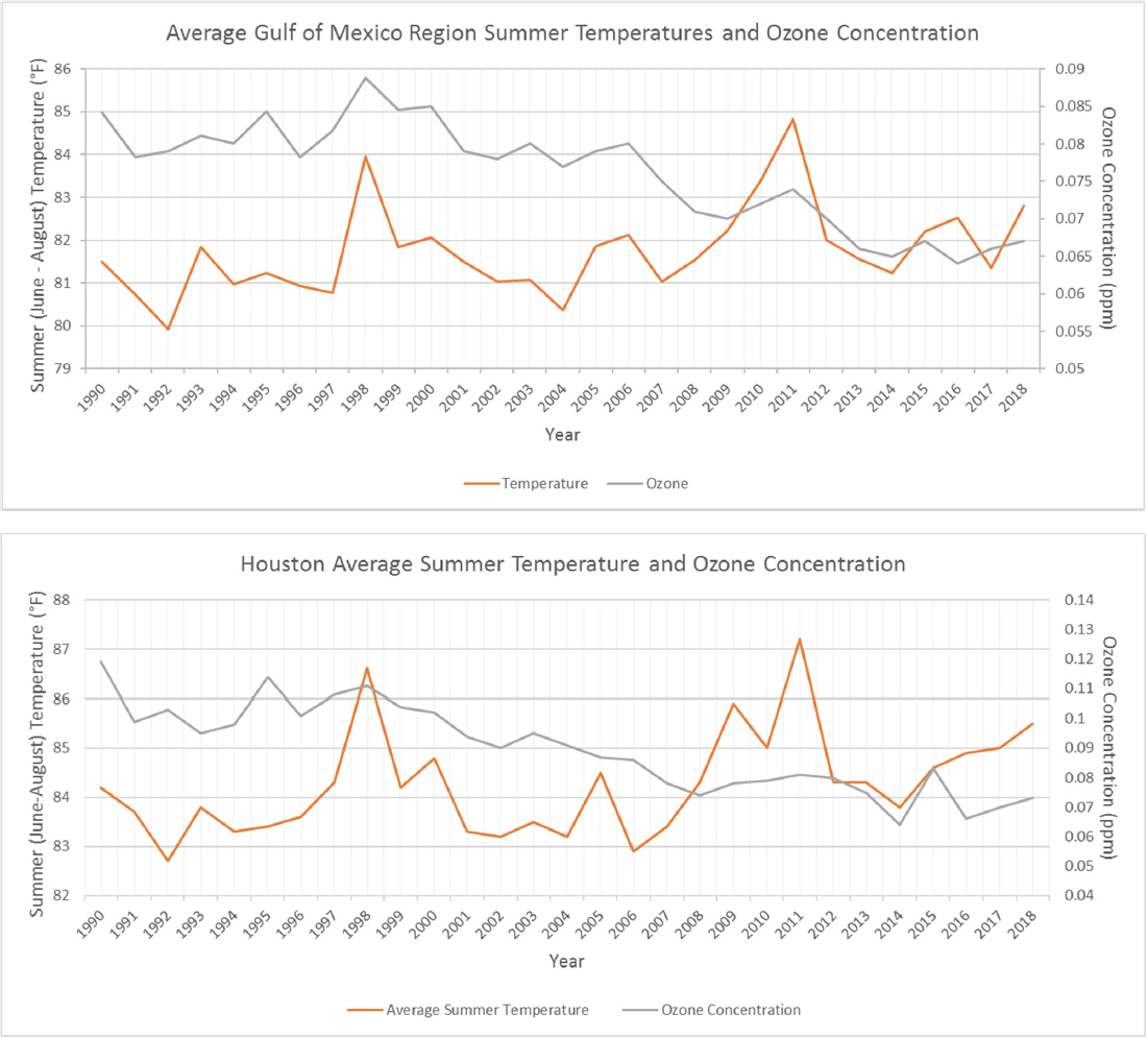
a The averaging time for ozone is the annual fourth-highest daily maximum 8-hour concentration. Generated with data from the U.S. Environmental Protection Agency (EPA; https://www.epa.gov/outdoor-air-quality-data) and the U.S. National Oceanic and Atmospheric Administration’s (NOAA’s) National Centers for Environmental Information (https://www.ncdc.noaa.gov/cag). See Appendix D for data.
___________________
a The resulting regression between ozone, temperature and year over the period shown is (with the standard errors in parentheses): [O3]= 1739 – 0.87 (0.095)*year +1 (0.54) TEMP R2=0.75 The reason for the high intercept is that the “year” variable starts in 1990.
The study’s choice of 2012 for the base year has implications for the development of the new EETs and contributes to the committee’s finding that the new EETs are not protective of the NAAQS for ozone, PM2.5, PM102 (see review of Chapter 5). The main secondary pollutant of interest in the Gulf States is ozone. For this pollutant, the design values are defined as the annual fourth highest 8-hour average mixing ratio averaged over 3 years. Exceedances of the NAAQS are thus caused by exceptional conditions, and the committee notes that agencies such as the U.S. Environmental Protection Agency (EPA) and the California Air Resources Board would specifically model exceptional years in their air quality assessments.
As noted by EPA in their Appendix W document, it is important that the worst-case atmospheric conditions are identified and assessed for screening methods (EPA, 2017). EPA also suggests that base years chosen for regulatory modeling practice be an NEI year. The NEI was readily available for 2011, but the Study authors had to adjust the 2011 inventory to 2012 because of the choice of base year.
Conducting dispersion modeling using 5 years of meteorological data (2010-2014) appropriately captures a large range of conditions both conducive and less conducive to higher concentrations of primary pollutants. However, by choosing 2012 as the base case year, worst-case conditions are not used for ozone, PM2.5, and PM10 (the Study did not conduct modeling of secondary PM10 for EET development)3. This choice (and the Study’s formulation of the CART analysis approach as discussed in the review of Chapter 5) leads to the Study’s effective lack of an emission limit for secondary PM2.5 and PM10, and ozone precursors. The thresholds for emission exemptions for VOC, SOX, and NOX (Tables 5-21 and 5-22 of the Study4) are far greater than the emissions expected from any possible project and, in most cases, even the 10-lease scenario (Figure 4-1 of the Study). Furthermore, as noted in the review of Chapter 2, the meteorological fields had high biases in the wind speeds, likely enhancing dispersion.
___________________
2 Footnote added January 2020: Unless otherwise noted, this report refers to both primary and secondary PM.
3 Text modified January 2020 to acknowledge that the Study did not conduct modeling of secondary PM10 for EET development.
4 Page, line, figure, and table numbers are for the version of the document that BOEM provided to the committee in June 2019. This version is available through the National Academies Public Access Records Office: https://www8.nationalacademies.org/pa/ManageRequest.aspx?key=51411.
REVIEW OF THE EXECUTIVE SUMMARY
The Executive Summary captures the report as it is currently written. Specifically, it provides accurate summaries of each chapter. However, it does not fully capture the linkages between the Study report chapters and analyses, and how the results and methods developed will impact air quality management in the region. The Executive Summary could be improved by providing a clear statement of the Study’s objectives and how and where they were addressed. In addition, the Executive Summary would be more useful if it provided a strong “big picture” view and synthesis of the report, including material in the appendices.
REVIEW OF CHAPTER 1: INTRODUCTION
The introduction chapter provides a study overview that is specific to the Study as reported. The chapter begins with a discussion of the Bureau of Ocean Energy Management (BOEM) requirements for prescribing regulations for the OCS, including areas of jurisdiction, and a discussion of the air quality regulations that are the subject of the modeling conducted. It notes a number of non-attainment areas in the region. Furthermore, it lays out the air quality modeling needs.
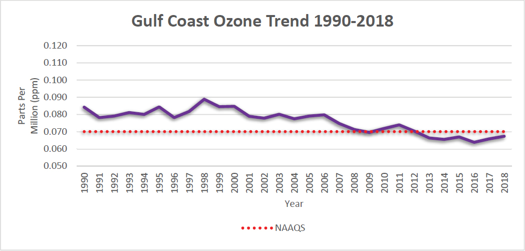
The chapter could be strengthened in two key ways. First, it should state the study objectives, linking to where those are addressed in the Study report. This should be as specific as practicable. Second, it should provide a discussion of some overarching issues related to air quality management in the GOMR that are of importance to understanding the full Study report. For example, a discussion of historic and forecasted future trends in oil and gas exploration, development, and production operations and the associated emissions would help provide greater context for the Study. This would include the trends in near-shore versus deep water drilling. A summary of air quality trends in the GOMR should be included (see Figure 2.3 for an example), as well as the specific research that has been conducted to quantify the impact of offshore emissions. Furthermore, “big picture” discussions of the use of Significant Impact Levels (SILs), Prevention of Significant Deterioration increments, and EETs would be helpful in providing important context.
REVIEW OF CHAPTER 2: WRF MODEL PERFORMANCE EVALUATION
Meteorology in the Gulf of Mexico Region and Its Impact on Air Quality
Meteorology in the GOMR is very complex. It is characterized by land-sea interactions, sea breeze circulation, surface temperature contrasts, and a complex coastline, which result in a warm, humid, subtropical climate with moderate rainfall. There is a range of weather conditions that affect the air quality of this region. Geography complicates the influence of these weather systems, leading to differences in the local meteorological conditions within the GOMR.
Due to differential heating between the land and the waters, a shallow wind system develops in the GOMR. During the day, the air temperature above the land is typically higher than that over
the water because land heats up more rapidly than water. However, during the night, the converse is true; the air temperature above the water is typically higher than that over the land because the land surface cools more quickly than the water. These temperature differences result in a circulation system that affects the direction of transport. Depending on the direction of winds and recirculation processes due to land-sea breeze, the resulting mixing can advect pollution from offshore sources toward coastal areas during the daytime.
Therefore, accurate representation of the diurnal cycle in land-sea breeze circulation is a key to model development in the GOMR. Another important feature to capture in the meteorological models is the spatial variation along the Gulf coast, which results in strong regional and local meteorological trends.
The Lake Michigan Ozone Study5 has been the basis for various air quality modeling studies that have demonstrated that synoptic forcings such as land-sea breeze, seasonal variations, and atmospheric stability together affect plume transport and lead to patterns such as fumigation and looping (Kitada, 1987; Lyons et al., 1995). Meteorological characteristics, including recirculation of ozone due to land-sea breeze and frontal passage, (Morris et al., 2010; Rappenglück et al., 2008) temperature, (Nielsen-Gammon et al., 2005), height of the planetary boundary layer (PBL; Berman et al., 1999), and subsidence (Zhang and Rao, 1999) can result in high ground ozone concentrations and mixing of ozone. The Rappengluck et al. study (2008) is particularly relevant to the Study as it found that ozone exceedances in the Houston region were largely due to recirculation processes within the land-sea breeze system.
In general, meteorological errors can contribute significantly to bias in the air quality models (Cheng et al., 2007; Heidorn and Yap, 1986; Robeson and Steyn, 1990). Meteorological metrics that are important for modeling offshore dispersion sources to onshore locations include wind field, temperature profiles, water vapor mixing ratio, atmospheric stability, boundary layer depth, turbulent fluxes, surface pressure, clouds, shortwave radiation in the lowest 2 or 3 km of the troposphere, and the amount and timing of precipitation. Parameters that influence the performance of meteorological models include the model initial conditions, physical process parameterizations, and spatial and temporal resolutions.
PBL processes are always important for pollution scenarios. They influence the lower atmosphere turbulence and thus the transport and mixing processes; capturing the diurnal variation of PBL is directly relevant to dispersion studies. Currently, it is challenging for WRF simulations to capture the stable PBL height and nighttime surface inversions over land. Furthermore, for air quality model calculation of deposition fluxes (wet deposition in particular), it is important to accurately predict the amount and timing of precipitation (Appel et al., 2011; Qiao et al., 2015).
WRF GOMR Dataset Evaluation and Development of New WRF Dataset
The Study conducts a performance analysis on two existing 2011 WRF datasets. One of the datasets was generated by the EPA’s Office of Research and Development Atmospheric Modeling and Analysis Division in Research Triangle Park, NC, and covers the conterminous
___________________
United States using 12-km grid resolution. The other WRF dataset was developed specifically for the GOMR by ENVIRON in the 12-km and 4-km domain. The analysis presented is similar to ENVIRON’s previous 2001 report (Emery et al., 2001). In fact, the committee noted that large portions of text from the Emery report appear in the Study’s Appendix B-1. In scientific writing, this is generally frowned upon unless the text is in quotes. The authors should correctly cite the use of text from prior works, their own or others.
Based on the results from their evaluation of the existing WRF datasets, the Study authors decided to develop a new 5-year high-resolution WRF dataset. The evaluation of the existing datasets presents errors and biases of wind speed, wind direction, and temperature as WRF performance benchmarks categorized for simple and complex domain conditions.6 The Study authors conclude that the errors and biases are outside the “acceptable conditions” for a few of the months in the dataset and that the datasets would not accurately represent the overwater portions of the Study area.
Performance Evaluation of the New WRF Dataset
Neither the model physics nor the model evaluation was performed with sufficient rigor to demonstrate that the newly developed WRF data capture the key physics that can advect pollution from offshore sources toward coastal areas. The Study’s model evaluation also does not capture the impact of the bias and errors from the meteorological data to the dispersion models.
The 5-year meteorological trends including frontal passage, land-sea breeze circulation, stalled stationary front marked by light and variable winds and low mixing depths, and the role of the synoptic wind field should be the starting point of the meteorological analysis in the GOMR. This is missing in the Study’s analysis. As noted above, the air quality of the GOMR is influenced by large-scale synoptic forcings, orientation of the frontal systems, a variety of fronts (warm, cold, and stationary), and the speed of frontal systems. A comprehensive analysis of meteorological trends and metrics that influence the transport of pollutants would provide a more direct evaluation of dispersion modeling errors and bias. In particular, the following are the concerns noted:
- The Study does not include seasonal, year-to-year, and 24-hour variation analysis of the errors and frequency of unstable and stable events, as well as the regimes of stability, which are primary meteorological features in the GOMR. What are the seasonal patterns of the winds, humidity, surface air temperature, and direction of the fronts?
- The Study does not include meteorological metrics, including PBL height, diurnal patters, and errors in vertical profile. Given that the WRF data serve as input to the dispersion models, it is important to include these meteorological metrics at different locations along the Gulf coast for meteorological conditions where offshore pollution dispersion to onshore is dominant.
___________________
6 Complex and simple conditions refer to the modeled terrain. Simple conditions are flat topography with no roughness. Complex conditions include topography such as valleys, hills, etc.
- The model evaluation does not evaluate combinations of metrics, nor does it encompass the entire 5 years of data that include significant events specific to the GOMR. A time series for the full 5 years and diurnal patterns of PBL height, temperature, and wind speed are missing. It is common practice to compare PBL metrics with observations at a different frequency than the input variable used in the model. This enables evaluation with and without specific observation data (e.g., to remove data from surface observation stations). An understanding of the meteorological trends from the available data would provide guidance to modelers on such evaluation (e.g., meteorological conditions that enhance the offshore pollution transport to onshore locations).
The Study reports onshore and offshore errors and bias in wind speed, direction, and temperature:
- WRF has shown a tendency to have biases in wind speeds in various conditions. Current literature (e.g., Wyszogrodzki et al., 2013; Zhang et al., 2013) indicates that WRF model errors and biases behave differently according to the time of the day, seasons, and geographical (topography and land uses) contrasts. A more comprehensive review of the literature of WRF model performance in similar situations to the Study would be informative as to how well the model should capture the observed meteorologies and the potential impacts of the biases. Sensitivity studies to better estimate the effect of biases in meteorological parameters on predicted concentrations and EETs would be informative as well.
- The Study’s onshore results indicated a positive bias in wind speed and temperature for 2013-2014, which is outside the complex region during the winter months in the refined region. More importantly, the root mean square (RMS) errors in wind speed were around 2-3 m/s for average wind speeds less than 10 m/s. The committee questions the impact of this high wind speed bias and high RMS error during the winter months. The Study does not report the error analysis for offshore data for the coarse domain (i.e., 12-km domain). The Study should conduct an error analysis for different stability regimes as this type of analysis will identify the stability regimes that WRF significantly deviates from. The observations from field measurements should guide the cases to be selected for model evaluation (different stability regimes).
- Several factors may lead to cumulative error in the dispersion modeling analysis: (a) the high sensitivity of the 4-km domain to PBL schemes, input/boundary data and nudging, and cloud microphysics; (b) the positive wind speed bias; and (c) the wide spread of the wind directions outside the simple region for most months. It is important to understand the relation of the errors to the atmospheric stability.
Finally, there is a clear need for better observations (or model predictions) of sea and near-surface air temperature differences in the Gulf of Mexico between the pollution sources and the coast. Data assimilation is one method for reducing model biases by improving the quality of initial conditions. By taking advantage of the new observational technologies and advanced data assimilation techniques (e.g., an off-line high-resolution land-surface model), or the initialization of the model through assimilation of diverse observations, the model-forecast errors could be further mitigated.
Specific Comments on the Newly Developed 5-Year WRF Dataset
To develop the new dataset, the Study uses WRF version 3.7 with one-way nesting of grids with a resolution of 36, 12, and 4 km with the finest resolution centered on the coastal region and overwater portions of GOMR and with 37 vertical layers.
- The Study authors selected North American Model (NAM) data to provide initial and boundary conditions to the WRF model as it has a lower error and bias compared to the other methods. The NAM data were reanalyzed and then nudged to guide the WRF model. This will likely lead to errors in the initial and boundary conditions. The Study authors should nudge the reanalysis/observation data and then compare the datasets to be selected for initial conditions and boundary conditions.
- In the GOMR, the WRF model is very sensitive to sea-surface temperature; however, the Study does not include a discussion on the quality of the selected sea-surface temperature dataset.
- The evaluation metrics do not include parameters, including PBL height, which is an important WRF performance metric. Furthermore, the committee is skeptical that the Yonsei University WRF PBL model is the best option for this Study. For example, it is not clear if the Yonsei University model in the Study includes a top-down mixing due to radiative cooling.
- The Study finds that onshore and offshore error/bias of wind speed, wind direction, temperature, and humidity are within the bounds of complex conditions for most of the months. However, the errors in wind speed and wind direction for offshore are much higher compared to onshore as seen from the error/bias as well as wind rose plots. The comparisons are based on 2010-2014 averaged wind observations, which does not give sufficient confidence in the data. As this domain is prone to high stability conditions, inversion layers, and low-level jets, identifying the frequency of such events and comparison for these events is essential in the GOMR regime. The time series analysis of error/bias for stability regime and model evaluation of a combination of metrics, including PBL height, is more suitable for the GOMR.
- An instantaneous hourly output is stored for analysis instead of using an hourly averaged output. Based on existing work, it is possible to generate hourly averaged data using WRF modifications. Given that the GOMR is prone to high gradients and strong inversion conditions, it is not clear how much error/bias is generated by not using the hourly averaged data for dispersion studies in the Study. A sensitivity analysis for land-sea surface behavior and PBL model is missing and this raises concerns about the confidence in the generated data. The Study should generate hourly averaged output instead of instantaneous hourly output and address the impact of hourly averaging on the dispersion model.
- Section 2.3.4 of the Study only compares total amount of precipitation with observations but does not include any evaluation of the timing of the precipitation using surface observation data. As the air pollutant concentrations change with time, it is important to ensure that the precipitation occurs at the right time with the right amount so that the wet deposition of air pollutants can be properly calculated.
REVIEW OF CHAPTER 3: EMISSIONS INVENTORY FOR THE CUMULATIVE AND VISIBILITY IMPACTS ASSESSMENT
The authors of the Study made a significant effort in developing the emissions used as inputs in the modeling of cumulative air quality and visibility impacts. While the NEI was readily available for 2011, the Study argues that the modeling should be performed for 2012. As a consequence, the 2011 inventory needed to be adjusted to 2012. In addition, the authors developed emissions for most of the sources related to fossil-fuel production on OCS, and also developed emissions for the Mexican part of the different modeling domains. Over the course of this work, the authors needed to make many choices regarding the modeling years, emissions scenarios, and emissions factors.
- In its review of Chapter 3, the committee has some concerns regarding uncertainties and possible biases in the emissions that followed from the choices made by the authors.
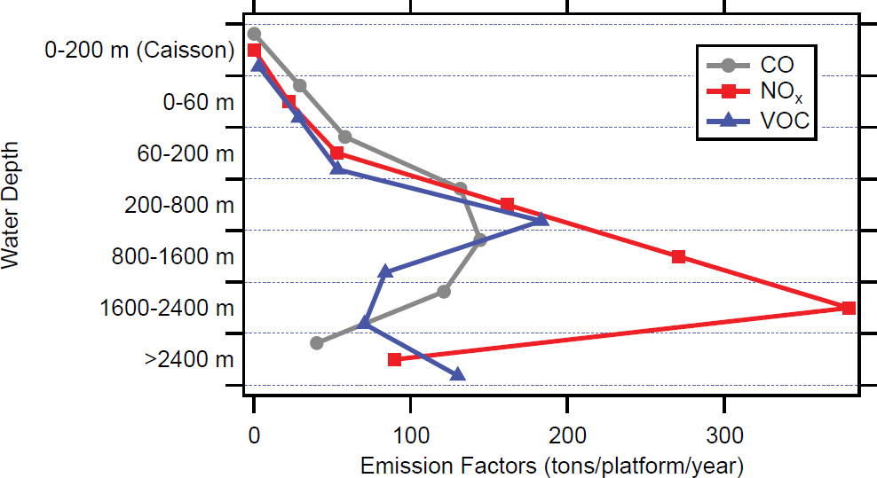
- factors for offshore oil and gas exploration, development, and production have not been widely studied, and the data that are included in the Study raise some questions. For example, in Table 3-6 of the Study emission factors for production platforms are presented in units of tons per platform per year (see Figure 2.4). The committee is struck by the Study’s finding that emission factors of CO and NOX peak at different water depths, while emission factors of VOC show local maxima at two different depths. The committee is not questioning the care and detail that went into the development of these emission factors. However, the apparent incongruity between the emissions of different pollutants does raise a question about the accuracy of these emission factors, and would benefit from additional explanation in the Study.
- There is an extensive body of literature that has been used to evaluate emission inventories using top-down methods. For example, emissions of NOX in the NEI-2011 inventory were evaluated during the National Aeronautics and Space Administration’s Studies of Emissions and Atmospheric Composition, Clouds and Climate Coupling by Regional Surveys mission over the continental United States in 2013 and were found to be biased high by 30-60% (Travis et al., 2016). Biogenic emissions in the Southern United States were evaluated using NOAA and National Science Foundation airborne measurements and the Model of Emissions of Gases and Aerosols from Nature (MEGAN 2.1) inventory used in the Study was found to be systematically higher than the Biogenic Emissions Inventory System (BEIS) inventory (Wang et al., 2017; Warneke et al., 2010). Emissions of highly reactive VOCs from the petrochemical industry along the Houston Ship Channel, which were shown to be of key importance for ozone formation in the Houston area (Wert et al., 2003), have been shown to be systematically underestimated, sometimes by more than an order of magnitude (Mellqvist et al., 2010; Ryerson et al., 2003). These studies are not referenced in the Study but should be used to acknowledge and address uncertainties in the modeled emissions.
Scenarios of Lease Sales
The authors specifically analyze two future emissions scenarios in which a single lease or nine additional leases for new oil and gas development are sold in the 2017-2022 period. The committee notes that emissions in the single-lease scenario rose sharply in a few years (Figure 3-7 of the Study), while emissions in the 10-lease scenario rose much more slowly (Figure 3-6 of the Study). The committee does not question the care and detail that went into calculating these emission scenarios, but the figures do bring up questions about how sensitive the emissions are to assumptions in the calculations.
The Study uses an overly specific and perhaps biased scenario of lease sales. It is unclear to the committee what the likelihood is of a scenario where 10 leases are sold in 2017-2022, but no new leases are sold from 2022 until 2036, which is the year the future model analysis was done. The committee recognizes that such sales are uncertain, as are the associated emissions. However, not considering their potential impact will bias the results. Since this review took place in 2019, and thus already halfway through the 2017-2022 period, actual lease sales could be compared against assumed lease sales in the model. The committee also notes that actual lease sales have been in
deep water,7 while the scenario presented in the Study appears to have many lease sales in shallower waters (Figure 3-9 of the Study) and thus closer to the continent, thereby potentially overestimating the air quality impacts.
The Study also finds that existing OCS emissions can contribute substantially (up to >14 ppb) to elevated ozone levels in the Houston region (which is a non-attainment area). Furthermore, future lease sales could contribute more than 5 ppb of ozone in the Houston region and to nitrogen deposition above the deposition analysis threshold in Class I and II areas in the region.
Finally, the continental emissions in the 2036 scenario are those used for the 2017 modeling. Decreases in NOX emissions from mobile, off-road, and point sources between 2017 and 2036 are thus ignored, which possibly biases the ozone model calculations high.
Finding: The Study uses an overly specific and perhaps biased scenario of lease sales; in particular, the scenario does not include emission-generating activities associated with potential future sales after 2022.
Recommendation: A future update to the Study should evaluate the impacts from other scenarios for continued exploration, development, and production of oil and gas reserves on the outer continental shelf beyond the 2017-2022 lease-sale scenarios.
___________________
7 See https://www.boem.gov/GOMR-Historical-Lease-Sale-Information.
Specific Comments
- A new rule for sulfur emissions from marine vessels was introduced in 2012, i.e., during the base model year. This leads to a potential uncertainty in SO2 emissions during the transition period, which is not addressed in the Study.
- The Study assesses emissions from helicopters using an estimated number of trips and emission factors from Switzerland. An important detail is whether or not the helicopter traffic takes place in the marine boundary layer or further aloft. This question is only addressed by a brief comment in the Study.
- Ammonia emission factors for offshore oil and gas are from a 1994 report. Is there any reason to believe that these have/have not changed since then?
- In Section 3.4.3 of the Study, the text mentions that the ship emissions are based on the Automatic Identification Systems (AIS). The earlier text suggested that the AIS data had not been used.
- The Study does not address VOC speciation in any sort of detail. Clearly the reactivity and potential to contribute to ozone formation vary greatly for different VOCs, and without specific information the committee cannot comment on the accuracy of the assumed speciation.
- The reference for the adjustment to diesel fuel sulfur content should be Section 3.4.4 of the Study, not Section 3.4.3.1 (which does not exist).
REVIEW OF CHAPTER 4: CUMULATIVE AND AIR QUALITY IMPACTS ANALYSIS
This Study chapter describes the cumulative photochemical air quality impact analysis for the future year 20178 using an emission inventory projected from the base year 2012 for two different lease sale scenarios (single sale and 10-lease sales). It begins with a summary of the preparation of meteorology and emission dataset for CAMx modeling. Model performance evaluation for criteria pollutants is conducted using the photochemical modeling results for 2012 based on the base case emission inventory. The chapter moves on to assess the future year air quality impacts with respect to the NAAQS criteria pollutants as well as sulfur and nitrogen deposition and visibility using the source apportionment modeling results. Lastly, it briefly discusses the potential factors that lead to uncertainties in model simulations.
As noted previously, the choice of 2012 as the meteorology modeling time period may not be the most appropriate to assess the impact of offshore OCS activities on ozone, particulate matter (PM), and visibility.
___________________
8 When the Study was conducted to evaluate the future year impacts associated with implementation of the Proposed Action for the 2017–2022 OCS Oil and Gas Leasing Program, emissions were projected from the base year to 2017, which was considered a future year with respect to the base year 2012.
Air Quality Model Performance Evaluation
The discussion of air quality model performance contains numerous errors and omissions. Concentration units should be used for RMS error in Table 4-9 of the Study instead of percentage. Also, fractional bias (FB) and fractional gross error (FE) as defined in the Study’s Table 4-9 should be more accurately called “mean fractional bias” and “mean fractional error.”
EPA guidance also recommends that the correlation coefficient or coefficient of determination be included in the model performance analysis (EPA, 2018).9 However, Table 4-9 does not include this and the subsequent analyses in the Study do not report this model performance criterion. In the introduction part of Section 4.5.3, the Study states that current EPA guidance recommends FB/FE and normalized mean bias/normalized mean error (NMB/NME) as the preferred statistical measures. However, such a statement cannot be found in the latest version of the EPA guidelines or in the reference (EPA, 2014) cited by the Study. In contradiction, in the subsequent model performance analysis, the authors continue to use NMB and NME to evaluate ozone performance.
The Study includes performance statistics for both hourly ozone and daily maximum 8- hour average ozone for cut-off concentrations of 0 and 60 ppb in Table 4-11. This practice follows the EPA recommendations, but it would be more complete if the Study included a discussion of these EPA recommendations in the introduction on pages 175-176. In the discussion of EPA performance guidelines (p. 176, l. 10-23), the Study cites Boylan and Russell (2006) and Morris et al. (2009a,b). However, these references are not EPA guidelines. Table 4-10 listed ozone and PM performance goals and criteria. It should be modified to include proper references. In general, ozone and PM model performance analyses are done for quarterly and annual periods.
Since the study is focused on emissions over the GOMR, the model performance evaluation should be more focused on the days when the meteorological conditions are favorable for transfer of emissions from the GOMR to areas where onshore monitors are located for a more direct evaluation of the quality of the emission data over the GOMR. There are several techniques that the Study authors could consider to identify such days. For example, back trajectories that originated from each receptor can be calculated based on modeled or reanalysis data to select the days when back trajectories pass through the vicinity of known offshore sources in the GOMR. Since source apportionment simulations have been carried out, the Study authors could also select the days based on the source apportionment results—the days with higher contributions to modeled concentrations can be selected for model performance analysis. Different sets of days might be identified at different receptor locations.
In addition, the Study mentions that hourly PM measurements have also been used in the analysis (p. 173, l. 1-8), but the Study does not include the model performance evaluation of these hourly data. However, these data represent an important supplement to the low temporal resolution data based on federal reference method (FRM) and should be included in the model performance evaluation to further establish the confidence in the model performance. Section 4.5.3 should be revised to correct the errors and include additional model performance analysis for the period when the stations are affected by onshore flow.
___________________
9 The draft version of the EPA report was available during the Study’s timeline. The recommended metrics in the draft and final EPA report are the same.
Specific Comments
- Biogenic emissions in the Study are generated using MEGAN v2.1. However, as noted in the review of Chapter 3, it has been demonstrated in several previous studies (e.g., Wang et al., 2017) that default MEGAN inputs for North America lead to significantly high biases in the modeled biogenic emissions in the southeastern United States and can potentially affect ozone simulations. On the other hand, the BEIS simulated biogenic emissions have been shown to better agree with observations. Justification is needed for the selection of MEGAN over BEIS for biogenic emissions and uncertainty analysis should be conducted to evaluate how this would affect model simulations of ozone, PM2.5, and PM10.
- Chlorine (Cl) emissions have been demonstrated to affect ozone formation in Texas (e.g., Chang and Allen, 2006). However, it is not clear if the Study includes anthropogenic Cl emissions from various sources. The Study’s modeling exercise appears to consider particulate Cl from sea salt particles. The Study should consider additional Cl emissions from anthropogenic sources, especially in the coastal areas and over the OCS activity regions.
- The Study states that the CAMx model is configured for two-way (p. 166, l. 27) nesting but the WRF model is configured as one-way. In most off-line air quality modeling studies, the WRF model is configured for two-way nesting while the air quality model is configured for one-way nesting. The Study needs to further explain this uncommon choice in the configuration of the models.
- The Study states that the CAMx model includes a patch that is designed to increase the transport of pollutants from PBL to free troposphere (p. 168, l. 18-24). This patch concerns the committee because it appears to be an unjustified attempt to tune the model predictions. Apparently, the model was overpredicting concentrations, and a quick fix is to move some of the pollution up out of the PBL. The committee considers this to be the type of correction that should go through careful justification using the literature, peer review, and evaluation with field data.
- Nitrate and sulfate deposition fluxes are calculated in the base case model and used in the source apportionment analysis. However, it is unclear if the CAMx deposition module currently includes treatment of sub-grid variation in the dry deposition velocity due to variations in the land use/land cover. Such treatment is available in recent versions of the Community Multi-scale Air Quality (CMAQ) model, but it is unclear if CAMx includes such a capability and if so, whether it is used in the modeling exercises.
- Section 4.5.2 of the Study states that data from three NADP sites are used to evaluate the modeled wet deposition for nitrate and sulfate within the 4-km domain. The locations of these three sites should be illustrated on a map.
- NO2 and NOy concentrations in the 4-km domain are biased high in the simulations (Figure 4-23 of the Study). The Study attributes this high bias to overestimation of the mobile source emissions in the NEI. This is consistent with other top-down evaluations of NEI-2011 NOX emissions (Travis et al., 2016). The Study should address the implications of over-estimated NOX emissions and provide a literature review to support this (e.g., the magnitude of NO2 and NOy bias reported in this Study versus in other
- studies of the region). Similarly, the magnitude of overpredications of nitrate (Figure 4-24 of the Study) should also be compared with previous studies.
- Figure 4-25 of the Study shows significantly high biases in the simulated SO2 in the 4-km domain. The associated text (p. 192), however, does not provide reasons for why SO2 levels are biased high in the model.
- SO4 deposition was biased low in the simulations. The cause of this bias should be better analyzed. For example, a literature review could indicate whether such a bias is consistent with previous studies.
- It is not clear from the Study whether post-processing is applied to adjust the modeled PM2.5 semi-volatile NH4NO3 so that it can be more consistently compared with the PM2.5 concentration data in the AQS based on FRM. Such a treatment is included in the CMAQ post-processing procedure and should be applied in the PM2.5 model performance analysis.
- In 2012, high ozone concentrations were simulated over the Gulf of Mexico and significant contributions were found to be due to new offshore emissions. The Study correctly states that there is not sufficient observational evidence to support this. Additional on-site ozone monitoring should be carried out in future studies.
- Visibility model performance was not evaluated. Airport visual range data have been used in the past to evaluate model performance on low visual range days. The Study should evaluate the ability of the model in simulating visibility.
- The Study calculates the contributions of the OCS platform and support vessels to ozone future year design value increases using the source apportionment results. The Study separately calculates the contributions of the OCS platform and the OCS platform + supporting vessels. Table 4-16 of the Study only lists the total contributions of the OCS platform + supporting vessels. It would be clearer if contributions from the OCS platform and the supporting vessels were reported separately.
- The discussion of uncertainty (Section 4.8) is very brief and non-quantitative, particularly for the ozone modeling. There are large biases in the key precursors (e.g., NOX) and it is difficult to perform a complete uncertainty analysis for complex Eulerian models such as CAMx. Thus, the Study should perform additional simulations that consider different emission scenarios (or adjustments) of the precursors to provide more quantitative uncertainty analysis. NRC (2007) provides more discussion on quantifying and communicating uncertainties and should be reviewed by the Study authors.
REVIEW OF CHAPTER 5: EMISSION EXEMPTION THRESHOLD EVALUATION
Appendix W Equivalency Demonstration
In general, the models used in the Study are consistent with 40 CFR part 51, though it is noted that EPA delisted CALPUFF and does not make a recommendation for a specific photochemical grid model. CALPUFF was delisted because it was viewed by EPA as not needed, as opposed to being delisted for any technical issue, and the photochemical grid model used in the Study (CAMx) is applied extensively nationwide. EPA does not have guidelines for the use of any models by BOEM for modeling in the GOMR, as that is under the authority of BOEM. In April 201210 and as updated in August 2019,11 the BOEM director approved the use of OCD at distances offshore of up to 50 km and CALPUFF for distances beyond 50 km.
The Appendix W Equivalency Demonstration applied to justify the use of the WRF- Mesoscale Model Interface (MMIF)-AERMOD method over BOEM’s regulatory default model (OCD) and the WRF-MMIF-AERCOARE-AERMOD method did not meet the "performs better” criteria. The Study concludes that BOEM should use the EPA regulatory default dispersion model for over land (AERMOD) for source-receptor distances overwater of fewer than 50 km, in place of the current BOEM-approved model, OCD (which has not been updated in the past few decades). The Study conducted an extensive analysis of the performance of the OCD, AERMOD, and CALPUFF models using tracer data from overwater dispersion experiments in Louisiana (Cameron) and California (Carpinteria, Pismo, and Ventura). None of the models were able to consistently reproduce tracer studies of atmospheric dispersion to within a factor of two. The Study concludes that: “No dispersion model is a clear outperformer when the results from the four tracer studies are considered together.” Furthermore, it concludes that: “In general, Table 2 through Table 5 (of Appendix E-1) show that AERMOD and CALPUFF are able to simulate the short-range dispersion from offshore emission sources just as well as the regulatory default model, OCD. No model clearly outperforms the others at all tracer study locations, suggesting that the configurations specific to each tracer study (e.g., source-receptor distances, complex terrain) influence each model differently.” The transport distances for these four studies ranged from 0.8 to 10 km (Wong et al., 2016), and the Study points out the clear research need for GOMR-specific tracer studies of atmospheric dispersion at great distance from shore in order to better evaluate the models. Wong et al. (2016) conducted a similar analysis of OCD, AERMOD, and CALPUFF but used observed meteorology from the overwater dispersion experiments rather than output from the prognostic meteorological model WRF. Wong et al (2016) found better agreement between the three models and with the tracer data (Figure 9) than the Study (Figures 9 through 15 of Appendix E.1). Wong et al. (2016) rarely had models disagree with each other or the tracer data by more than a factor of two, while the Study had many discrepancies greater than a factor of two. These discrepancies are especially pronounced for the Carpinteria and Pismo Beach overwater dispersion experiments, and should be investigated by the Study authors.
The Study conducted a synthetic source modeling study for offshore distances of 20 and 40 km and found that: “Overall, there is better agreement between AERMOD and OCD concentrations than between CALPUFF and OCD, especially for the highest concentrations, which carry the most weight for regulatory purposes” (EPA, 2014). However, there can be differences in
___________________
10 See https://www.boem.gov/Approved-Air-Quality-Models-for-the-GOMR/.
estimated concentrations of up to several orders of magnitude (Figures 25 to 56 in the Study’s Appendix E-1) between the models at mid-to-lower concentrations (presumably receptors at longer distances from the synthetic sources). Depending on the source type, CALPUFF can be either much lower or much higher than AERMOD. Thus, a modeling discontinuity, potentially several orders of magnitude in either direction, arises at offshore distances of 50 km, inside of which AERMOD is favored and beyond which CALPUFF is used. The Study did not conduct modeling at this distance from shore and states that: “no conclusions can be drawn from this report regarding the performance of CALPUFF in situations where the BOEM administrator has already approved its use (greater than 50 km, matching EPA Guidance).” The very large differences between OCD, AERMOD, and CALPUFF found for the synthetic sources is very puzzling in light of the general agreement seen for the four overwater dispersion experiments by both the Study and by Wong et al. (2016). This should be investigated by the Study authors.
It could be argued that, for consistency, CALPUFF be applied at the full range of distances (greater and fewer than 50 km) because it is the only model capable of modeling dispersion at scales of a few tens of meters to many kilometers. Another advantage is that the CALPUFF version (5.8.5) used by the Study contains the PRIME downwash algorithm that can explicitly deal with elevated platforms and accept over-water turbulence formulations. An alternative for a conservative screening approach is to run all three models and select the largest of the predicted concentrations at various distances.
Emission Exemption Thresholds
The emission exemption thresholds (EETs) are a screening tool, taking into account distance from shore and projected annual emission estimates in exploration, development, and production plans by potential lessees and operators, to determine if more refined air quality modeling and emission controls are needed. They are used to determine whether the emissions levels of a proposed new source exceed a Significant Emission Rate that will in turn lead to shoreline concentrations that exceed the NAAQS pollutant’s SIL. These SILs are determined by EPA and are often just a few percent of the NAAQS limits.
BOEM is currently using EETs that were developed in the 1980s, apparently without detailed air quality modeling nor consideration of any long-term NAAQS (Box 2.2). They clearly need to be updated to reflect newly regulated pollutants (i.e., PM2.5 and PM10) and updated (i.e., 8-hour-average ozone, 1-hour-average NO2 and SO2) air quality standards as well as state-of-the-science dispersion and photochemical models.
The committee’s understanding from its public discussions with both BOEM and industry representatives is that the typical lessee/operator response to an EET limit that is exceeded is to reduce oil and gas throughput (and thus projected emissions) rather than conduct refined modeling and implement emission controls. This means that less conservative threshold limits will likely lead to higher allowable emissions (especially NOX) and associated air quality impacts. This may be particularly true for the NOX EET based on the 1-hour-average NO2 NAAQS, which is generally the most limiting due to the relative stringency of that NAAQS and high NOX emissions from diesel and natural gas engines.
The Study developed five emission scenarios for small-, medium-, and large-scale operations (15 in all), placed these synthetic sources at distances varying from 4 to 242 statute miles from shore in the Western and Central Gulf, and modeled shoreline impacts. These results were used to evaluate the existing EETs and as input into approaches to develop new EETs. The committee has three sets of concerns with the Study’s approach for developing and applying the new EET methods.
First, the approach to the emissions applied to the EET formulas may lead to a bias. BOEM allows potential lessees/operators to use annualized emissions, rather than daily maximum emissions, for the short-term NAAQS EETs. This contrasts with the appropriate use of maximum hourly emissions required by BOEM for subsequent air quality modeling of proposed projects that exceed one or more EETs12. Furthermore, BOEM only counts vessel emissions within 25 km of the platform and assigns those emissions to the distance from shore to the platform, despite the fact that the vessels are primarily emitting at all distances between the platform and their ports.
Second, the cumulative effect of biases and uncertainties across the meteorological and emission datasets, and from the air quality models themselves, could be quite large and result in EET estimates that are both higher and lower than they should be. The CART-based PM2.5 and PM10 EETs are based on direct emissions of PM, and do not include secondary formation of particle nitrates and sulfates. Future updates to the Study should consider a formal error analysis that takes into account cumulative uncertainties from meteorological and emission inputs to the air quality modeling.
A third area of concern is the degree to which the new EET approaches continue to generate false negatives (i.e., instances where more refined air quality modeling or emission controls are needed, but the EET does not call for it). The committee’s understanding of the EET formulas as
___________________
12 Text modified January 2020. In discussions related to BOEM’s allowance of potential lessees/operators to use annualized emissions for the short-term NAAQS EETs, text was added to acknowledge that BOEM requires maximum hourly emissions for subsequent air quality modeling of proposed projects that exceed one or more EETs.
These results are similar to air quality modeling for EET evaluation performed by BOEM and its contractors in the Alaska OCS (BOEM, 2017). Surprisingly, almost all the false negatives generated by comparing the existing EETs to the new modeling occurred within 50 statute miles from shore, with no such cut-off for false positives (Figures E.5-1 through E.5-5 in Appendix E.5). The modeling discontinuity at 50 km is a possible contributing factor.
The large number of false negatives from the existing method for the short-term NAAQS does suggest that the EETs should be updated. While the Study developed several new versions of EETs, using both statistical and air quality modeling approaches, none of these are shown to be
protective of all NAAQS because of the continued existence of false negatives for several pollutants.
The Study proposes the CART approach to balance false positives and false negatives, but it is more appropriate to eliminate false negatives, based on EPA guidance and the objective of protecting air quality and public health.
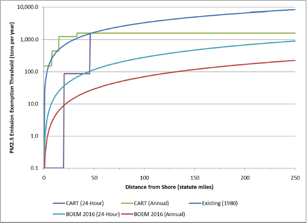
The CART analysis results in abrupt patterns that are physically unrealistic in comparison to the smooth curves generated from a series of EETs proposed in a still open rulemaking by BOEM (2016) based on Huang (2015) (see Figures 2.5 and 2.6). There are several cases where no emissions are allowed within a certain distance13. Another unrealistic result is a pattern where
___________________
13 Text and Figure 2.5 modified January 2020. In discussions related to examples of unrealistic patterns of the CART analysis, the original report incorrectly stated that there would be no emission limit for projects beyond a specific distance. The Study’s Appendix E (page E. 8-3) states: "maximum value presented in the emissions tables should be considered the upper limit of the decision trees." The two CART curves in Figure 2.5 are now capped with the maximum modeled PM2.5 emission rate of 45 grams per second (1564 tons per year) from the Study’s Table E.8-1.
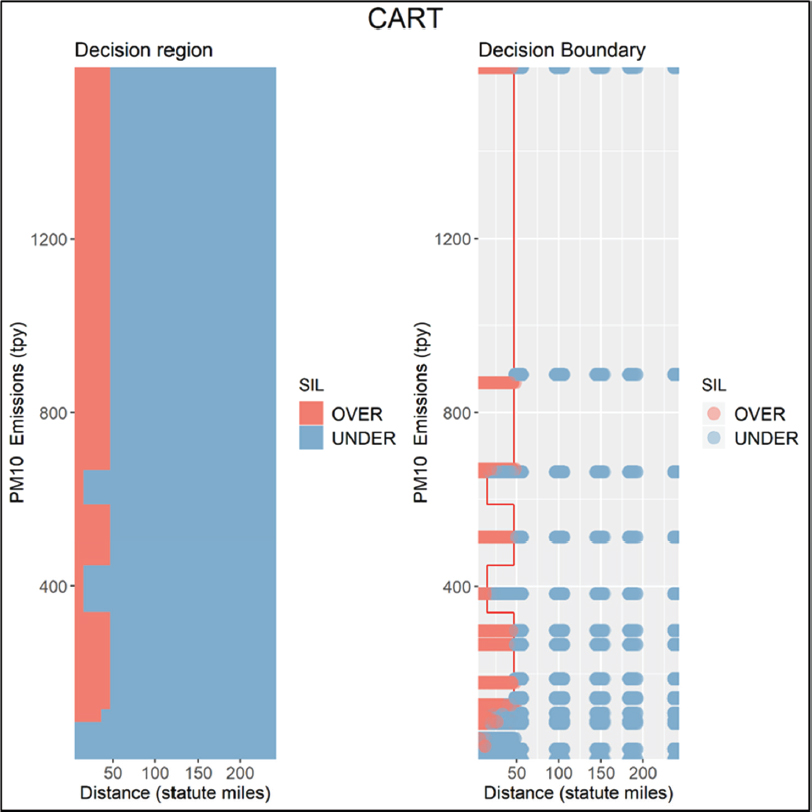
lower emissions are prohibited but higher emissions are allowed at the same distance from shore (see Figure 2.7). This is likely the result of relying on a limited number of emission scenarios, and the caveat in Appendix E.8.3 (“The CART analysis should not be extrapolated for emission values beyond what are presented in Tables E.8-1 and E.8-4.”) should be noted on each CART result, in consistent emission rate units. An important concern of the committee is that limitations of the EET methods should be clearly stated in the main body of the report and the summary, not just in an appendix.
Another possibility is the discontinuity created by using different models within and beyond 50 km. There may be problems with the application of the CART methodology itself, which is a nonparametric technique that must be used with care outside of the observed data. The five-fold cross validation used in the Study is one solution to this modeling issue, but does not go far enough. The Study should consider testing CART performance using out-of-sample data not used to develop the nonparametric model. The Study does not address whether the same data splits are used for each model comparison. In the cross-validation splits, if the number of points above and below the SIL are not controlled, one could end up with fitting the statistical model to very few concentrations above the SIL. The variability in the false positive and false negative rates for each cross-validation is not communicated, nor is the number of observations falling within each category of the decision tree.
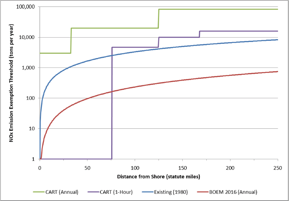
Another puzzle is that while the existing EETs for the short-term NAAQS exhibit false negatives ranging from 2% to 36%, the CART-generated EETs for NO2 (see Figure 2.6) are consistently higher at longer distances from shore. The Study authors should use caution in relying on decision trees that lack atmospheric physics- and chemistry-based insights, and scrutinize the use of branches in the decision tree that are not reflective of a specific physically and chemically realistic relationship between estimated maximum impact, the emissions level, and distance.
The Study suggests a potential alternative approach to the EET formulas that “estimate impacts based on comparable modeled sources. For example, an operator could identify a hypothetical source modeling run at a comparable emission rate and distance to shore as the proposed source to evaluate the likelihood of a significant impact.” The committee agrees that this approach holds promise and should be further investigated.
Searching for EETs that are protective of both short-term and long-term NAAQS is complicated in the GOMR because observations indicate that dispersion conditions over the GOM are unstable more than 90% of the time (Hanna et al., 2006). Thus, a particular shoreline-to-platform EET distance dependence that is appropriate for the long-term average NAAQS may prove inadequate for protection against short-term NAAQS violations associated with worst-case stable dispersion conditions occurring less than 10% of the time. In addition, near-shore assessments of overwater stability may not be appropriate farther from shore. Furthermore, Hanna et al. (2006) observed that prognostic model (Eta in their case) simulations of boundary layer wind speeds tend to exceed the wind profiler observations by 1-2 m/s near-shore and by 2-6 m/s at distances of 100-200 km offshore. Predicting higher than observed winds seems to be a persistent problem for prognostic models, particularly under low wind and low surface roughness conditions. It is unclear if (or how) WRF deals with this issue.
Thus, if a modeled concentration database is used to produce new short-term NAAQS EETs, a persistent offshore wind speed bias could undermine their validity. Even if onshore wind monitors correctly constrain the WRF winds, the speed slowdown from offshore to onshore does not lead to higher concentrations, as the convergence in the along-wind direction is compensated for by divergence in the cross-wind and vertical dimensions.
Also, the fact that stability might vary with distance from shore even in poor dispersion conditions suggests that an EET for the short-term NAAQS might require a more complex distance dependence, such as:
EET ~ Dp / [1 + (D/L)p-1/2], where D is the source-receptor distance, L is a length-scale of order 30-80 km, and the exponent p might be of order 1 to 1.5.
The committee found the current Chapter 5 plots (e.g., Figure 5-10 and additional plots in the Appendix of the Study) to be somewhat limited in usefulness as one does not know if the positive or negative miss is a miss by a small amount or a miss by a substantial amount. In a revision, the Study might contain plots of the computed emissions quantity ESER versus distance from shore, D, where ESER ≡CSIL / R, where CSIL is the SIL concentration and R is the modeled coupling coefficient, R = Cmod/Emod for a particular hour (or short-term period), where Cmod = modeled shoreline concentration and Emod is the assumed emission rate used in the modeling of that source. All of the essential information regarding the meteorology and dispersion rates obtained from the modeling is captured in the coupling coefficient, R, with the larger values of R representing the poorer dispersion conditions. Clearly, the larger the coupling coefficient R, the
smaller the predicted ESER (or preferred EET for that hour or short-term period) would be. The resulting scatter plot of ESER versus distance, D would potentially be very crowded with data points; however, a line drawn below all of the data would represent a curve that had no false negatives. One could then fit this curve to an appropriate function of D, so that one ended up with a true EET formula with no false negatives rather than end up with a CART decision tree. Note that it may be more convenient to consider a log-log plot of ESER versus D, as the lower values would be “less crowded” and all power law forms (i.e., Dp would show up as straight lines).
Specific Comments
P. 299 Table 5-11 of the Study. One of the column headings is likely Number of Y Grid Cells.
Figure 5-8 (page 307) of the Study. Is the Y-axis label correct? An NO2 concentration of 2 x 10⁵ μg per m3 equals 0.2 g per m3, which cannot be correct.
___________________
14 Text modified January 2020. In discussions related to examples of unrealistic patterns of the CART analysis, the original report incorrectly stated that there would be no emission limit for projects beyond a specific distance. The Study’s Appendix E (page E. 8-3) states: "maximum value presented in the emissions tables should be considered the upper limit of the decision trees."
REVIEW OF CHAPTER 6: UNCERTAINTY AND RECOMMENDATIONS
This chapter is rather short, particularly given the importance of the topic. In particular, no quantitative uncertainty analysis was conducted, and the uncertainties identified are typically more general and well known as opposed to being specific to the Study. Furthermore, as currently formulated, the uncertainty discussion tends to indict the study at hand, e.g., by saying that the “emissions inputs to chemical transport models such as those used in this study represent only rough approximations” and that “the gas and particulate phase chemical mechanisms
___________________
15 Text modified January 2020 to clarify that meteorological conditions that are most conducive to elevated levels of ozone, PM2.5, and PM10 are not used for EET development in the Study.
contained in these models do not reliably simulate the vast complexity…” If this is true, one wonders about the reliability of the Study, in general and for the results reported.
Statements regarding the uncertainties identified should also be more strongly supported. For example, the Study states that “The largest source of uncertainty in the EET modeling is in the representation of the universe of possible platform configurations and resulting emission levels possible from OCS sources.” The committee cannot identify where this is specifically demonstrated in the Study. Such a statement would require a well-formulated uncertainty study.
Identifying, and to the extent practicable quantifying, the sources of uncertainty in environmental modeling is critical for the use of those models in regulatory decision making (NRC, 2007). In general, the chapter does not fully characterize the multiple potential uncertainties and potential biases, and does not provide quantitative assessments of how such uncertainties would impact the use of the model results.
The structure of the chapter could also be strengthened. It should begin with uncertainties and then have a recommendations section. Furthermore, the emissions section should precede the modeling section.
CONCLUDING THOUGHTS
BOEM and its contractors conducted extensive emissions, meteorological, and air quality modeling to better understand the impact of current and potential future emissions from the OCS of the GOMR on air quality and to test EET approaches. In general, the committee found that the air quality modeling tools used were scientifically appropriate and well documented. However, certain aspects of the Study were found to lead to potential underestimates of the impacts of GOMR emissions on air quality and EETs that would not identify all cases where additional air quality modeling or emission controls are warranted. In particular, the Study chose a base year for ozone, PM2.5, and PM10 with more historically average or typical conditions, rather than focusing on those conditions that are most conducive to pollution exceedances. Furthermore, the EET development was not conservative and allowed for false negatives. Specifically,
- the meteorological analyses and photochemical modeling have not been evaluated for their performance of conditions typical of when offshore emissions would have the largest impact on air quality on land and during the most critical times,
- the choice of base year does not account for increasing temperatures resulting from climate change,
- future emissions are only included through 2022, meaning that potential emissions from 2023-2036 are not considered in the future case, and
- the CART approach for the EETs allows for false negatives and, in some cases, has physically unrealistic results.
As such, the Study’s current results have the potential to underestimate the current and future impacts of OCS emissions on air quality, visibility, and deposition. Furthermore, the EET methods developed are not fully protective of future emissions leading to increased high pollutant levels and potential exceedances of the NAAQS. The overall utility of the Study could be improved if the Study authors build off the extensive modeling and analyses that was already conducted and address the shortcomings outlined in this report’s findings and recommendations.
The Study authors are in a unique position to further advance our understanding of how OCS sources impact air quality in the GOMR and develop robust and protective EET approaches.
This page intentionally left blank.


