
– 3 –

Geospatial Analyses of Social and Demographic Conditions
Eddie Hunsinger (California Department of Finance) moderated the first use-case session of the workshop, focusing on implications for broader geospatial analyses of census data. Seth Spielman (University of Colorado) and David Van Riper (Minnesota Population Center) collaborated in an extended-length presentation. Some of the background material they presented on the geographic aspects of the Census Bureau’s planned Disclosure Avoidance System (DAS) was incorporated in Chapter 2’s overview of the methodology for a more coherent treatment. Nicholas Nagle (University of Tennessee) spoke about ramifications for place-level and school district-level studies, and Mark Hansen (Columbia Journalism School) offered remarks as lead questioner and moderator for the floor discussion session.
3.1 GEOGRAPHIC REVIEW OF DIFFERENTIALLY PRIVATE DEMONSTRATION DATA
Seth Spielman (University of Colorado) characterized this joint work with David Van Riper (Minnesota Population Center) as a geographic review, a set of exploratory spatial data investigations comparing the 2010 Demonstration Data Products (DDP) with the original 2010 Census publications.1 Their review included sweeping looks across various levels of geographic aggregation and
___________________
1 In closing their talk, Van Riper and Spielman said that all code and data related to this presentation would be posted at http://github.com/geoss/CNSTAT_DIFF_PRIVACY.
drilled down to metropolitan-scale measures of inequality between and within cities. Spielman set the stage for the presentation—and the remainder of the workshop—as a first cut at determining where the Census Bureau’s revised approach stands in terms of resolving the inherent tension between privacy and data availability and utility, and then turned the presentation over to Van Riper. Van Riper began by discussing the geographic hierarchy of levels, referred to throughout the workshop as the “spine,” as summarized in Section 2.1.2. In this session, Van Riper raised the point that the “off-spine” geographies include some very important legal and political entities, such as places (including incorporated cities), county subdivisions (including functioning townships in several states), American Indian and Alaska Native areas, and school districts. Such geographic levels are very consequential in people’s lives, Van Riper argued: “they implement policy, they enforce laws, they pass taxes.” They are, he argued, “just as important” as the on-spine geographies, yet their estimates in the 2010 DDP are subject to the aggregation of error and noise from component blocks. Accordingly, he said that this presentation would discuss these effects.
3.1.1 Residential Segregation
Van Riper worked through a series of metrics comparing the 2010 DDP and the original 2010 Census publications regarding their implications for assessing residential segregation, which he said that researchers commonly study by comparing census tract-level population characteristics to the population distributions that prevail in the core-based (or, in older terminology, metropolitan) statistical areas. He said that the analysis would focus on four mutually exclusive race/ethnicity groups: white non-Hispanic, black non-Hispanic, Hispanic (for all other race groups and combinations of race), and an all-other-race, non-Hispanic category.
Van Riper briefly described three scatterplots from this analysis, each focused on a different metric used in segregation analysis:
- The multigroup entropy index H, a measure of the distribution of demographic groups within an area; he did not have time to explain in the talk, but his slide notes indicate that the index ranges from 0 to 1, 0 connoting “complete segregation” and 1 indicating that “each census tract has the same population proportions as the [core-based statistical area] as a whole;”
- A multigroup spatial proximity measure (per the slide notes, essentially an average of demographic group sizes weighted by spatial distance between corresponding census tract centroids) that Van Riper said increases from a minimum of 1 (no clustering) as spatial clustering increases; and
- Morrill’s D (for which Van Riper said that he restricted attention to white non-Hispanics and African American non-Hispanics), which he said can be interpreted as the “percentage of the minority group [that] would have to move among census tracts so that each tract effectively has the same proportion as the [core-based statistical area] level;” he noted that the measure is known to be very sensitive to noise and measurement error, but that it has the desirable property of focusing on truly local comparisons, being premised on pairs of adjacent tracts.
The points Van Riper made in his presentation did not concern the meaning or policy interpretation of these segregation measures, but rather sought only to show whether the measures—points on a scatterplot corresponding to core-based statistical areas, the computed score from 2010 Census Summary File 1 (SF1) on the x-axis and the scores from the 2010 DDP on the y—generally fell on the 45-degree equality line. Van Riper found that the 2010 DDP data “match fairly well” with the results from the original 2010 Census tabulations, with the latter Morrill’s D graph showing the most tendency to stray from the line, while most values still reasonably clustered around it and a very few major outliers. He hastened to add that this could certainly change with different ϵ or constraints used to generate the privatized census data, but the behavior of these measures is “fairly reasonable” for the settings used in the 2010 DDP. Critically, he also attributed the general accuracy to the fact that the geographies used in these analyses are “on-spine,” census tracts (as a proxy for neighborhoods) being one of the DAS processing levels and core-based statistical areas being agglomerations of a relatively small number of (on-spine) counties. Time permitting, he said that he would have liked to have measured place-level segregation, using the off-spine geography of places (i.e., cities) as the denominator, to get a sense of those effects.
3.1.2 Differences by Geographic Level
Van Riper’s next set of analyses examined the effect of the DAS runs on off-spine geographies, which do not receive a direct allocation of ϵ relative to on-spine geographies. The four subplots in Figure 3.1 all consider the estimates at four on-spine geographic levels (state, county, tract, and block group) and two off-spine levels (county subdivisions and places). As an indicator of important differences, Van Riper chose a difference of 10 percent or more between the count in the 2010 Census SF1 and the count in the 2010 DDP. They also divided the geographic units into population deciles according to their population in the 2010 Census published data to further accentuate the effects.
For total population, no states are off by 10 percent or more (which is to be expected, as state total population was held invariant in the 2010 DDP), and the other on-spine geographies experienced very few 10-percent-or-more swings,
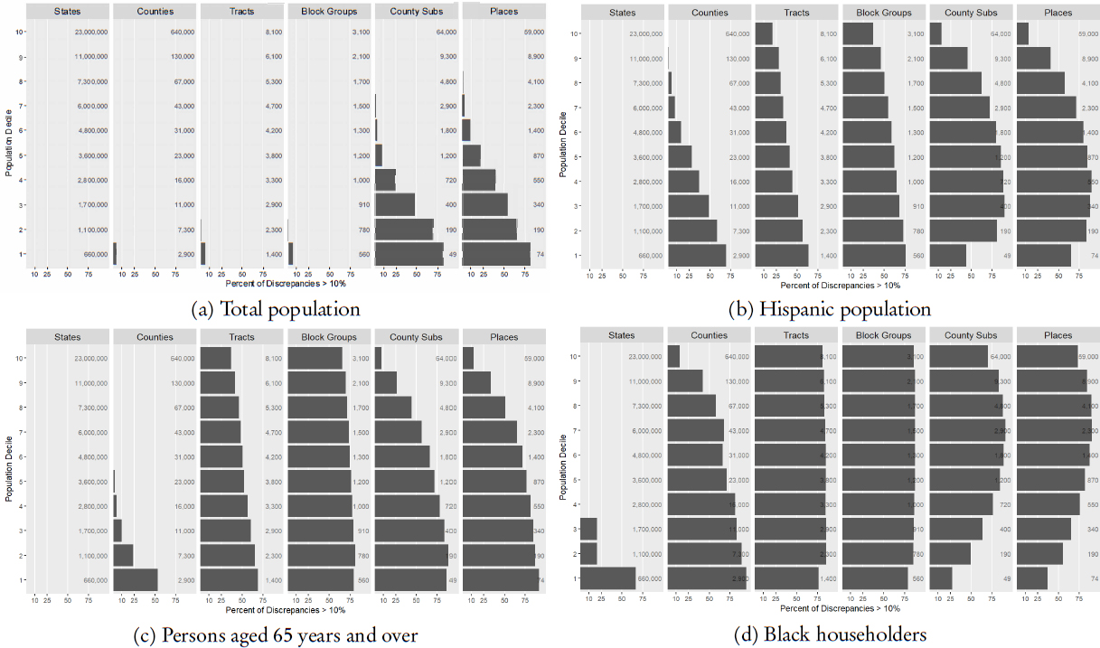
SOURCE: David Van Riper and Seth Spielman workshop presentation.
those for the least populous (deciles 1 and 2) levels. But “when you move to off-spine it doesn’t perform as well at all,” Van Riper said. In the first population decile, more than 75 percent of the least populous county subdivisions and places undergo differences of 10 percent or more—and, unfortunately, that extent of matching on total population “is really going to be your best case.” Figures 3.1(b) and (c) restrict attention to the Hispanic and over-65 populations, respectively, and for those demographic breaks, even the on-spine tract and block group geographies routinely experience population swings of 10 percent or more in the 2010 DDP relative to the original 2010 Census SF1 data. Shifting to the housing data in Figure 3.1(d), which focuses attention on African American householders (heads of household), even the least populous states become prone to major shifts of 10 percent or greater. In summary, he said, the off-spine geographies fare worse than the on-spine geographies, and the impact varies substantially by population size category.
3.1.3 Spatial Differences
Spielman resumed the presentation with a series of histograms computed over all census tracts that show the distribution in “gains” and “losses” in population between the 2010 Census SF1 and the 2010 DDP, confirming impressions already reached in the earlier presentations: for total population, white population, and Hispanic population, distributions concentrated tightly around 0. As a geographer, though, he said he was naturally concerned with the possibilities for spatial patterning that might underlie these balanced histograms. The same balanced histogram in the aggregate might mask very real pockets of concentration, areas where the population “gains” or “losses” are clustered or where they might just as well look like random static when analyzed spatially.
Accordingly, he argued for spatial analysis of the distribution of changes between the 2010 Census publications and the 2010 DDP—while conceding that he and Van Riper had only one map in this presentation slide deck. Moreover, he conceded that this map, a choropleth map of census tracts in the Washington, DC, area, color-coded to show decreases in white population in magenta and gains in white population in green, is only meant to be illustrative. Indeed, he said, it is “very hard to look at map like this and to tell if there is a pattern or not.”
Instead, Spielman suggested turning to an analysis of Moran’s I, a well-known and developed measure of spatial autocorrelation in the spatial statistics literature. Spielman described Moran’s I simply as “a correlation between the observed change in a particular tract and the tracts around it.” Pure spatial randomness would correspond to a Moran’s I score of 0, while absolute Moran’s I values greater than 0 would suggest the presence of spatial patterning. To see how the observed Moran’s I for tract-level differences between the 2010 Census
SOURCE: David Van Riper and Seth Spielman workshop presentation.
SF1 data and the 2010 DDP compares to true spatial randomness, Spielman and Van Riper ran simulation studies: randomly assigning the calculated differences by tract to all of the pertinent tracts, computing a new Moran’s I score, then repeating the random assignment 999 times.
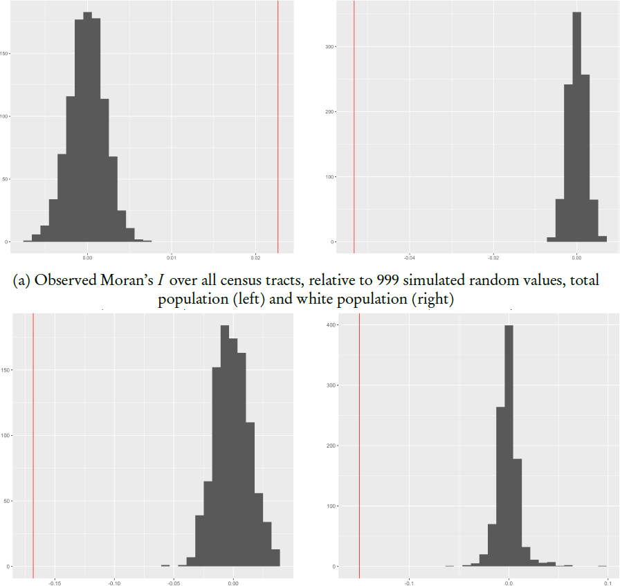
The results of the simulation testing are depicted in Figure 3.2. In all of the subfigures, the thin vertical (red) line depicts the observed value, which is plotted along with a histogram of the simulated scores for randomly assigned
tracts. This analysis is repeated for total population and white population at the national level in part (a) of the figure, for white population and African American populations in the state of Ohio in part (b). From this, Spielman suggested that the actual values of Moran’s I observed in the 2010 DDP relative to the 2010 Census products don’t have an intuitive meaning or speak to a possible cause for the patterning. What is clear from all of the figures is that the observed Moran’s I scores are distinctly different from the spatially random simulations and so are “not consistent with spatial randomness.” Again, exactly what the patterns are and how they might affect particular use cases of the census data awaits further investigation, but Spielman suggests that “certain places are gaining and certain places are losing” in a way that is “systematic within space” at the tract level, and that this may be problematic for local use cases of census data.
3.1.4 Closing Thoughts
Van Riper closed the presentation by itemizing some thoughts on the process and products ahead that he had developed with Spielman in preparing for the workshop. In terms of process, he asked what the process would be in the future for resolving and selecting the final DAS parameters and assumptions, and what the interaction would look like with data users, to get their input and feedback reflected in the final selections. Importantly, he also asked how the Census Bureau plans to educate users about this new approach and the resulting data: Will it fall to the Census Bureau to provide that explanation and education or to other parties who disseminate data and support data users?
More realizations of the DAS process on 2010 Census or other comparable data topped Van Riper’s “wish list” for additional products and information. “It’s difficult to make recommendations on an N of 1,” he noted, particularly when that single glimpse at the operation uses one set of parameters and assumptions. Absent more runs of the data being made publicly available, it’s difficult to offer suggestions about how the various levers at play might be pulled. Secondly, he observed that the results for off-spine geographic levels are sufficiently worrisome that they are something that is “going to have to get dealt with” through improvements in the process, particularly finding some way to get a dedicated ϵ allocation (a step toward better data quality) for those important geographies. Acknowledging the complications that Phil Leclerc and Matthew Spence noted when the question was posed to them (Section 2.3), he echoed the idea of imposing additional invariants in the population and argued for at least an empirical analysis of the effects on the privacy-accuracy tradeoff if block-level total population was made invariant. Finally, Van Riper said that the Census Bureau should work on metrics of uncertainty in the privatized data: given the knowledge, suggested in the presentation, that more than 75 percent of county subdivisions for some population deciles are “off” by 10
percent or more, it stands to reason that data users are going to need to know how uncertain the data may be.
He closed by observing again that this is difficult work, trying to balance the important public and private goods. His personal opinion and preference is to assign a lot more value to the accuracy side of the balance than the privacy side, but he said that the tradeoffs need to be fully elaborated and considered, and that the final decision-making process should be “participatory,” with data users having “a seat at the table” to give feedback to the Census Bureau. He warned that if the 2020 Census data end up emanating from an opaque, complicated, closed process that is not well understood by users (and, moreover, if those data run counter to local knowledge), there may be an irreparable break in the trust between the Census Bureau and its data users.
3.2 IMPLICATIONS FOR MUNICIPALITIES AND SCHOOL ENROLLMENT STATISTICS
Nicholas Nagle (University of Tennessee) began by observing that in the draft agendas for the workshop his topic was listed as “Implications for School Enrollment Statistics.” But, in the end, he said that his presentation would actually speak more to the implications for municipalities (the off-spine geographic level of places), though he would still offer an example of the use case of census data in school enrollment forecasting.
To vividly illustrate the pride that local governments take in their population figures and the degree to which that information has long been assumed to be trusted, public information, Nagle displayed a photo montage of road signs from around the state. These “welcome” signs to individual cities and towns routinely “advertise” the population total by including it on those signs. But, beyond civic pride, Nagle noted that place-level population totals mean real money to these localities. In particular, he displayed an excerpt from Tennessee state law governing the distribution of the state’s sales and use tax revenue, which it collects in lieu of a state income tax (Tenn. Code Ann. § 67-6-103(a)(3)(A)):2
Four and six thousand thirty ten-thousandths percent (4.6030%) shall be appropriated to the several incorporated municipalities within this state to be allocated and distributed to them monthly by the commissioner of finance and administration, in the proportion as the population of each municipality bears to the aggregate population of all municipalities within the state, according to the latest federal census and other censuses authorized by law.
By this provision—a statutory, nondiscretionary use of census data for automatic disbursement of funds—an important flow of revenue to local governments is explicitly linked to the relative populations of municipalities (places,
___________________
2 Nagle’s slides inadvertently gave the reference as Section 67 of title 67 of Tennessee Code.
SOURCE: Nicholas Nagle workshop presentation.
in the census lexicon) in the state. The amount varies from year to year, but Nagle suggested that the allocation is on the order of $115 per capita.
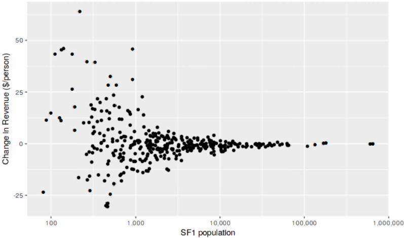
Nagle illustrated the impact of the 2020 DAS processing on the effective allocation of these state funds in two ways: a histogram of the effective allocation that Tennessee municipalities would receive under the 2010 DDP numbers (superimposing the nominal $115 average for reference), and—as shown in Figure 3.3—a scatterplot of the change in allotment by the population size of the municipality in the published 2010 Census data. The histogram shows a generally symmetric distribution around the nominal $115 amount, but tails of the distribution that suggest a somewhat disturbing range. “Every place is supposed to get $115 per capita,” he observed, “but the difference between winners and losers is just over $80 for the biggest ‘loser’ to $180 for the biggest ‘winner,”’ an almost two-times difference. The scatterplot in Figure 3.3 illustrates which municipalities would experience the “biggest distortions” in allocation, and it is the smaller-population facilities that are poised to see the greatest variability. Nagle said that he has heard much about the issues of bias (and unbiasedness) in the DAS process, but it is variability that is most concerning for small municipalities because of the potential for “tremendous inequities” in those places.
| City | Population | Change Per Capita | Revenue Difference | |
|---|---|---|---|---|
| 2010 SF1 | 2010 DDP | |||
| Henry | 464 | 338 | −$30.41 | −$14,112 |
| Guys | 466 | 346 | −$28.84 | −$13,440 |
| Winchester | 8,530 | 8,122 | −$5.36 | −$45,696 |
| Pulaski | 7,870 | 7,556 | −$4.47 | −$35,168 |
| Spring Hill | 29,036 | 28,560 | −$1.84 | −$53,312 |
| Columbia | 34,681 | 34,221 | −$1.49 | −$51,520 |
| Murfreesboro | 108,755 | 107,583 | −$1.21 | −$131,264 |
| Clarksville | 132,929 | 132,413 | −$0.43 | −$57,792 |
SOURCE: Nicholas Nagle workshop presentation.
Nagle displayed how these numbers look in practice for some of the municipalities that would lose revenue in Table 3.1. Small incorporated places like Henry and Guys would lose on the order of $30 per capita in state tax allotment, roughly $13,000 to 14,000 in overall revenue. However tempting it might be to think of these as “small” differences, it is vitally important to those communities. Nagle said that one of the two communities, Henry and Guys, has five local employees and the other seven employees, most of them part-time. These “small” revenue discrepancies make the difference between “whether or not they can afford to repave their roads each year, or whether or not they can afford to hire a full-time or part-time police chief.” Another city on the list, Spring Hill, ranks as one of the fastest growing communities in the nation, and it is fairly large compared to other Tennessee cities. Its projected change per capita under the 2010 DDP totals would be relatively small, but the revenue difference does not necessarily have a “small” impact. The same law that defines the allocation of state tax revenues to the municipalities also authorizes them to conduct up to four special censuses in each 10-year period. Spring Hill has done several of these special censuses, given its growth. But those special censuses can also be expensive and so are not a viable alternative for communities that may be unhappy with their U.S. census data.
Nagle briefly displayed an analysis of change in total population, from 2010 Summary File 1 to the 2010 DDP for all incorporated places in the nation, a subset of the overall place geographic level that excludes the census-designated places that are defined for statistical purposes. The scatterplot of the population change by the place’s population in the 2010 Census SF1 shows a distinct
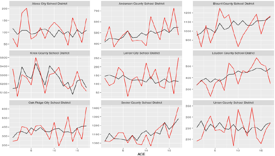
NOTE: Black line is the 2010 Census Summary File 1 count (tending to be smoother); red line is the 2010 Demonstration Data Product count (tending to be more jagged).
SOURCE: Nicholas Nagle workshop presentation.
increase in variability as the size of the place increases and also (by Nagle’s estimation, at place population of 150 or greater) a slight central tendency toward population loss in the 2010 DDP numbers. The mean population loss for an incorporated place in the 2010 DDP data is roughly 42 persons. Nagle reiterated his main point that these “errors” might not seem that great but they “absolutely matter” to the small places that rely on their counts for fund allocation purposes.
Pivoting to his originally planned topic, Nagle turned to another off-spine geographic level in school districts. In particular, he focused on school districts in his home county of Knox County, Tennessee. Of these districts, the Knox County School District itself has the largest service population; by comparison, the Alcoa City School District is a small one, numbering in the total population of hundreds of people. Plots of the counts of school-age children by individual years of age for both the 2010 Census SF1 and the 2010 DDP, are illustrated in Figure 3.4. Nagle’s basic point in presenting the data plots is the clear visual impression from the plots: the two plot lines do not track each other
particularly well except for the largest districts like Knox County School District itself. Moreover, the tracking is particularly poor in small districts like Alcoa City where, again, the magnitude of the differences may appear small but the practical difference between expecting 50 students next year or 200 is very consequential. Nagle alluded briefly to current efforts to quantify some of the differences relative to actual enrollment statistics for the school districts, but said that the work was hindered by not having access to exact 2010-vintage enrollment data. He said that he had to make some assumptions and adjustments for 2012 enrollment data, but even that preliminary work suggested a weakening in correlation with the enrollment data, 0.5 for the 2010 SF1 data and just over 0.3 with the 2010 DDP data.
Nagle drew the same conclusions as Van Riper and Spielman did, with some thoughts on process and products going forward. Nagle suggested that consideration be given to adding more invariants to the calculations. Total population by place may be one statistic with sufficiently many statutory uses that it should be afforded additional accuracy protection, somehow. Off the cuff, Nagle suggested another possibility: constructing a parallel data product that does nothing but generate total population counts for the off-spine geographies with a “government use,” including incorporated places and American Indian and Alaska Native reservation lands. A data product with no demographic and housing characteristics at all, only the total count, might be a “middle way” solution to the problem.
3.3 FLOOR DISCUSSION
Hunsinger turned the microphone over to Mark Hansen (Columbia Journalism School, Columbia University), who had been asked to serve as a “lead questioner” for this discussion session. Hansen began with a brief mention of work that he has been doing with a graduate student at Columbia: essentially replicating the Census Bureau’s own database reconstruction attack (Section 2.1.1) to derive an alternative microdata detail file. The goal would then be to use the Census Bureau’s public DAS code, with different parameterizations to generate not just one DDP but many demonstration products. This would help illuminate the consequences of different levels of noise injection and produce approximate measures of bias and margin of error.
Hansen directed the first question to Spielman and Van Riper, which was to provide some further discussion of the Moran’s I analysis. The earlier presentations had all suggested that small places tend to “estimate a little high, large places a little low,” so there is an implicit correlation with total population. It is well known that total population isn’t distributed across the nation with pure spatial randomness. So, is it any real surprise that the Moran’s I analysis suggested something other than pure spatial randomness? Spielman
replied that their analysis focused on the census tract, which is a somewhat special geographic level. There is, inevitably, variation in the population size of census tracts because of the way they nest within other levels, but they are a statistical geography constructed to be of roughly uniform size. At the least, there is less variation in the size of census tracts (due to the rules that govern their demarcation) than in other geographic levels, which partially suggests that Moran’s I is picking up on a different kind of systematic effect.3 Hansen followed up by noting that the scatterplots of core-based statistical areas suggested some distinct outliers, and asked whether Van Riper and Spielman had investigated those outliers for any common features. Van Riper said that they hadn’t looked at the outliers in a major way beyond spot-checking some particularly small micropolitan statistical areas. Those small statistical areas might yield “oddities” because they may be comprised of only two to four census tracts.4
Along similar lines, Hansen told Nagle that he very much appreciated Nagle’s putting the counts in “human terms,” or what they mean in the “life of the city.” In a follow-up to the question on outliers, he asked whether Nagle had looked into structures or commonalities among those “winners” and “losers” at the extremes of the distributions. Nagle replied that he had looked at which municipalities were winners versus losers in allocations but did not notice any key differences, which is in large part why he suggested concentrating on the variability more so than bias, because the variability creates inequity concerns.
Building on that theme, and repeating how impressed he was with the presentations given that “we were given picoseconds to pull these presentations together,” Hansen asked all three presenters what they would do if they had another six months to prepare for the presentations: What deeper things would you do as geographers to look at the data spatially? Van Riper answered first, indicating interest in calculating some of the local measures of segregation discussed by Reardon and O’Sullivan (2004), particularly those that allow constructing “surfaces of segregation across space.” He said that he has obtained the code to be able to replicate those measures, but it involves conversion from substantially older versions of ArcGIS software, and so it awaits future work.
___________________
3 Later in the discussion period, Mike Ratcliffe (Geography Division, U.S. Census Bureau) corroborated Spielman’s statements, saying that census tracts are suggested to range from 1,200–8,000 population with a target or optimal population of 4,000. But, recalling Figure 2.1, tracts are nested within counties so if a county has less than 1,200 population, the constituent tract(s) will necessarily be smaller than 1,200. Likewise, he said that the Census Bureau began working with some local planners to define tracts with more than 8,000 people—in the interest of resolving some concerns that arose from margins of error in American Community Survey data. Historically, though, the idea has been to impose some uniformity in defining tracts. Census block groups, another purely statistical geographic level, range in population from 600–3,000 but have no set “optimum” size, Ratcliffe said.
4 Later in the discussion period, Mike Ratcliffe corroborated this definition, with micropolitan areas being formed around defined “urban cores” of 10,000 people.
Spielman replied that he saw a more immediate need to articulate the full set of use cases and begin exploring how changes in the data introduced by the DAS changes may affect heretofore unanticipated uses. He said that he imagined there to be a “vast sort of semi-hidden group of people who use Census data every day to make decisions and do their jobs.” Having experienced similar kinds of issues when higher-variance estimates from the American Community Survey (ACS) entered circulation, Spielman worried about the Census Bureau and the data user community repeating past mistakes. In the absence of good education on and orientation to the ACS data, people somewhat “ignored the changes in the data and just kind of did what they have always done.” Nagle replied that he had been thinking of the temporal question rather than the spatial question—that is, there are important time series questions in characterizing uncertainty in the long-term, across-decades shifts in allocation that localities may need to contend with, where “they could win the Census lottery one decade and lose the Census lottery the next decade.”
Building on Spielman’s point, Hansen asked about the notion that had come up about presenting an uncertainty metric with census tabulations: “this, plus or minus something.” Would that actually help or, as experienced with the ACS, would people “just interpret the middle point and away we go” again? Nagle answered that in the revenue allocation context he had been working with, states would almost certainly “rather have a certified answer than something with a plus or minus.” Spielman agreed, saying that focus group and other work that he had done concerning the margins of error presented with ACS estimates is that “almost universally they ignore it.” Consistent with Nagle’s remarks, he said that a common refrain in that research is that “federal grant programs don’t take the margin of error into account.” Because the grantmakers effectively discard margin-of-error information, applicants disregard it as well. He hastened to add that he still thinks that uncertainty metrics and margins of error are good things and thinks they should be pursued, though they aren’t an automatic fix. Hunsinger said that in the grantmaking context, he has encouraged local communities to use the margins of error in building their cases for appeal, so that kind of role for the metrics may yet come to the fore.
Mike Ratcliffe (Geography Division, U.S. Census Bureau) said that he had to thank the people working in differential privacy in the 2020 Census for “teaching us a new term”—Census geographers had always spoken of the “central nesting hierarchy” but never the “spine” or the on-spine/off-spine distinction. In addition to corroborating some of the geographic concepts that had been described in the previous presentations, Ratcliffe put on the table that there had already been discussion of census blocks adding up to higher geographic levels and that this was likely to continue over the workshop. This frequently creates the mistaken impression, however, that the most atomic level of census geography (blocks) is constructed first and everything else is built up from that. “The reality is the opposite,” Ratcliffe argued: all of the other
geographies, on- and off-spine, are generally defined and updated first, and the intersections of those higher-level boundaries and features are used to form and revise census blocks.
Tommy Wright (U.S. Census Bureau) said that he wanted to share a true story, the memory of which was inspired by Nagle’s presentation on the allocation of tax revenues in Tennessee. Before joining the Census Bureau, Wright lived in Farragut, Tennessee, near Knoxville. Shortly after the 1990 Census, the city of Farragut could see that the town was growing rapidly, in ways that they worried might not be captured in the 1990 enumeration. Wright described how he served as an enumerator in a subsequent special census of Farragut, enumerating 19 housing units in his neighborhood counting 51 new people. The size of the neighborhood or tract was about 4,000 and, at that time, the per capita allocation was something like $75 or $86 rather than the current $115. His experience corroborated Nagle’s statements about small differences in population being very consequential to municipal leaders and city revenue streams. Nagle said that Farragut carried out another special census in the 2010s because of its continued growth, and he reiterated his concern that many localities may seek special censuses “just to get what they feel they deserve,” but that many of these communities are “least able to bear the burden of the cost” of recounts.
Gwynne Evans-Lomayesva (National Congress of American Indians) thanked the presenters for their examination of off-spine geographies, given her particular concern for the off-spine geography of American Indian and Alaska Native lands. She asked Nagle if he had any further ideas on solutions for producing accurate data (related to voting representation, funding formulas, and tribal governance) in off-spine areas. Nagle replied that he is still thinking through these matters, but again stated the possibility of “separating the number of people”—the count—“from their characteristics” in the differential privacy processing. Perhaps the Demographic and Housing Characteristics (DHC) files need not exactly correspond to the “o cial population,” and the details might be interpreted as separate products. He said that the notion of separate products might be a useful workaround to the problem of creating many more invariants if the invariant approach is unduly problematic. Nagle also reiterated that the broader data user community needs to take seriously the “challenge” of articulating their use cases to the Census Bureau. Van Riper said that he wanted to “push back” a little on Nagle’s point, because “the American Indian and Alaska Native population” and “the total population residing in American Indian and Alaska Native areas” are not equivalent concepts—but both are vitally important, and possibly both important to funding and other formulas.
Abraham Flaxman (University of Washington) commented that special censuses are a big interest in Washington State as well, and he said that one point that he wasn’t able to pack into his own workshop presentation (Section 5.4) was the way in which the new DAS approach might change
“strategic considerations” at the local level as to when to conduct these special censuses. He asked the panelists for any further thoughts on the general problem of instilling more confidence in the total population counts, whether through imposing additional total-count invariants or, as Phil Leclerc had suggested (Section 2.3), allocating the privacy-loss budget ϵ to provide more protection to the total counts. Nagle replied that it may be most important to determine which numbers are really “baked into the system” through statutory uses to get a better sense of exactly which estimates are in greatest need of that additional protection.
Xuemei Han (Fairfax County government, Virginia) said that, from the local government and local planning perspective, the importance of the tables in the DHC file (and the historical SF1) shouldn’t be minimized—those characteristics data are also used on a day-to-day basis. In particular, Han said, we use the number of households with children under 18 years old to decide where new schools are needed and to allocate the roughly 60 percent of state revenues that goes to the public schools. The county uses the data on households with 7 or more persons to identify areas of overcrowding and to target housing affordability programs. Han said that, looking at just those two variables, the 2010 DDP data for census tracts are “not usable”—all of the census tracts in the county “get either doubled or [halved], 50 percent of the number” in the 2010 SF1.
Qian Cai (University of Virginia) expressed additional concern that some of these discussions run counter to the extensive communications now underway to promote the 2020 Census. There are many complete count committees, extensive outreach on television and radio, all emphasizing the importance of the census and ensuring that everybody gets counts “only once and in the right place.” Cai said that she worried about how we promote counting “in the right place” in the context of the fact that the data eventually reflect noise-injected totals and plus-or-minus uncertainty. Nagle joked that, in his collaboration with the state, they are not seeking to widely publish in local media the variability in per capita revenues that was presented here in the workshop: “we are waiting until Census Day.”
Nancy Krieger (Harvard T.H. Chan School of Public Health) closed the discussion period by cautioning that attention shouldn’t be focused exclusively on “what currently is in statutory use,” because there are inequities that are “baked into the system” as well. The danger is in “enshrining past inequities going forward” rather than taking the opportunity to redress them.


