
Appendix C
Contemporaneous Correlation SUR Model
This appendix presents Zellner’s Seemingly Unrelated Regression (SUR) model and several extensions (Judge et al., 1985, pp. 28–29, 465–471; Zellner, 1962). The SUR method could help fishery managers improve the precision (reduce the percent standard errors [PSEs]) of annual or in-season catch forecasts made using MRIP output estimates of catch and associated PSEs. The SUR method would likely be most useful when there are relatively large correlations in the catch errors of forecasting models across MRIP domains.
The SUR model is a type of generalized least squares (GLS) regression model (Aitken, 1936; Hansen, 2007). A SUR model consists of a set of regression models, estimated jointly. In general, consider a system of M “stacked” linear regression forecasting models corresponding to M domains. The M domains could be M states, M substate regions, M species, M fishing modes, etc., or any combination of these domains. The M models are indexed:
i = 1, 2, ..., M
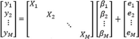
For each of the M models, there are T observations (corresponding to T time periods) on dependent variable yi, a matrix of nonstochastic independent variables Xi, a column vector of parameters βi to be estimated, and a column vector of errors ei. Each Xi matrix has Ki independent variables (columns). (Note that the numbers of, and the identities of, the independent variables may differ across the M models.)
![]()
where yi and ei are each of dimension (T×1), Xi is (T×Ki) and βi is (Ki×1). The M models can be written together in “stacked” matrix form as:
Alternatively, the set of M models can be written more compactly as simply:
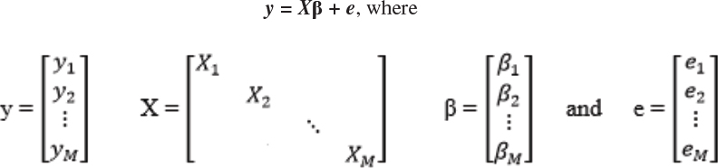
and where
- in a fisheries application, yi is the catch of species i, and y is a random vector of the yi;
- βi is the column vector of parameters for equation i, and β is the concatenated vector of all of the βi vectors;
- E(y) = Xβ0 for some β0; and
- variance-covariance matrix var(y) = Ω is a positive definite matrix.
In fishery applications, the matrix X could include such variables as:
- MRIP domain indicator (“dummy”) variables: geographic region, wave, fishing location (in/offshore, exclusive economic zone), fishery (recreational/commercial), mode (shore, private boat, charter);
- ancillary variables: weather, ocean conditions, unemployment rate, fuel prices, dummy variables for alternative fishing regulations, etc.; and
- the lagged values of the X variables listed above.
In the basic SUR model, the error in each equation (each domain) in the model is allowed to have a different variance. That is, the model accommodates heteroskedasticity across domains (Duncan, 1983).
In addition, the errors are allowed to be “contemporaneously correlated” across the equations (across domains) in the model; that is, the errors are correlated across domains at a given point in time. (In the basic SUR model, the errors are not autocorrelated across time; as noted below, however, extensions of the basic model allow the errors to be autocorrelated across time as well as contemporaneously.) Hence, the covariance matrix of the joint fish catch distribution vector y in the basic SUR model is given by:
![]()
where ![]() is the Kronecker product operator, I is the identity matrix, and:
is the Kronecker product operator, I is the identity matrix, and:
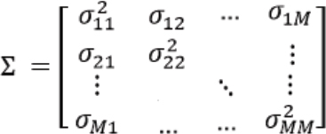
where ![]() is the error variance of model equation i, σij is the covariance in errors between model equations i and j at a given point in time (representing the contemporaneous correlation between domains i and j at that point in time), and σij = σji.
is the error variance of model equation i, σij is the covariance in errors between model equations i and j at a given point in time (representing the contemporaneous correlation between domains i and j at that point in time), and σij = σji.
It is important to recognize that fishery managers can obtain the elements of the matrix from MRIP. ![]() is the variance of the catch estimate for equation i (i.e., for domain i), and σij is the covariance in the catch errors across equations i and j (i.e., across domains i and j).
is the variance of the catch estimate for equation i (i.e., for domain i), and σij is the covariance in the catch errors across equations i and j (i.e., across domains i and j).
The best (minimum variance) linear unbiased estimator (BLUE) for β is (Aitken, 1936):
![]()
with variance-covariance matrix:
![]()
ABILITY OF SUR METHODS TO LOWER THE PSEs OF CATCH FORECASTS
Joint estimation of systems of multiple equations using SUR methods will in general lead to efficiency gains (greater precision, lower PSEs) relative to single-equation estimation (Zellner, 1962). Judge et al. (1985, p. 468) describe the types of situations in which the SUR method is likely to provide efficiency gains: “efficiency gains from joint estimation tend to be higher when the explanatory variables in different equations are not highly correlated but the disturbance terms corresponding to different equations are highly correlated.”
HYPOTHESIS TESTS FOR CONTEMPORANEOUS CORRELATION
Hypothesis tests exist for determining whether contemporaneous correlation is present and the SUR model may be warranted (e.g., Breusch and Pagan, 1980; Judge et al., 1985, p. 476).
SUR MODEL WITH AUTOCORRELATION (JUDGE ET AL., 1985, P. 518)
The SUR model can be extended to include autocorrelation in the errors over time within a domain (e.g., autoregressive, AR-1 models) (Judge et al., 1985, p. 483; Kmenta and Gilbert, 1970). The autocorrelation specification can be extended further to include higher-order autocorrelation (AR models), moving-average errors, and autoregressive moving-average models of the errors within each domain (Judge et al., 1985, p. 496). If the autoregressive specification is extended still further such that the error in a given domain is allowed to depend on the errors in previous time periods in all domains included in the model, the vector autoregressive model results (Judge et al., 1985, p. 484).
To fix these ideas, consider an example with just two domains (M = 2, m = 1, 2) and two time periods (T = 2, t = 1, 2). In this case:
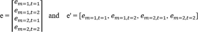
and hence variance-covariance matrix (Judge et al., 1985, p. 581):
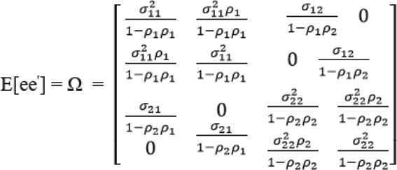
where, in the variance-covariance matrix above:
 is the variance for domain m = 1;
 is the variance for domain m = 2;
- σ12(same as σ21)) is the covariance between domain m = 1 and domain m = 2;
- ρ1 is the first-order autocorrelation coefficient for domain m = 1; and
- ρ2 is the first-order autocorrelation coefficient for domain m = 2.
The variance-covariance matrix above allows for:
- different variance for different domains (heteroscedasticity), that is,
 ;
; - autocorrelation across time within each domain, that is, ρ1 ≠ 0 and ρ2 ≠ 0;
- different autocorrelation for different domains, that is, ρ1 ≠ ρ2; and
- contemporaneous autocorrelation across domains, that is, σ12 ≠ 0 (same as σ21 ≠ 0).
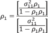
Autocorrelation coefficients can then be obtained by taking ratios of the appropriate elements of the variance-covariance matrix, for example:
VECTOR AUTOREGRESSIVE SPECIFICATION
With the last autocorrelation specification (Ω) above, the error within a domain at one point in time is affected by the error within that same domain from the previous point in time, but it is not affected by the error in the other domain at the previous point in time. If the error within a domain at one point in time is allowed to be affected by the error within that same domain from the previous point in time and the error in the other domain at the previous point in time, the VAR specification for the variance-covariance matrix results in:
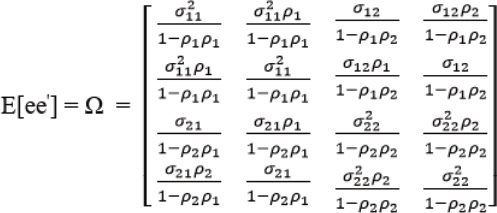
Again, the above example is for the case of two domains and two time periods. However, the matrix equations given above readily extend to any number of domains and time periods.
FURTHER EXTENSIONS OF THE BASIC SUR MODEL
The SUR model can also be extended to include unequal numbers of observations across equations (Judge et al., 1985, p. 480), as might be the case when one is combining information from multiple surveys that collect data with different frequencies or surveys that started or stopped at different points in time, or when bad weather interrupts data collection in a particular location and time period.
Wang et al. (1980) show how the SUR model can be extended to include lagged dependent variables (such as past values of catch and effort) and autocorrelated errors. So, for example, past values of catch and effort (along with other variables) could be included in the model to help predict current and future values of catch.
Ozuna and Gomez (1994) provide an example of using SUR to estimate fishing effort using a Poisson model of angler fishing effort. The SUR model can also be implemented within a Bayesian modeling framework (Judge et al., 1985, p. 478; Zellner, 1971, Chapter 8) (see Appendix D).
REFERENCES
Aitken, A. C. 1936. On least-squares and linear combinations of observations. Proceedings of the Royal Society of Edinburgh 55:42–48.
Breusch, T. S., and A. R. Pagan. 1980. The Lagrange multiplier test and its applications to model specification in econometrics. Review of Economic Studies 47:239–253.
Duncan, G. M. 1983. Estimation and inference for heteroskedastic systems of equations. International Economic Review 24:559–566.
Hansen, C. B. 2007. Generalized least squares inference in panel and multilevel models with serial correlation and fixed effects. Journal of Econometrics 140(2):670–694.
Judge, G. G., W. E. Griffiths, R. C. Hill, H. Lutkepohl, and T.-C. Lee. 1985. The Theory and Practice of Econometrics, 2nd Edition. New York: Wiley.
Kmenta, J., and R. F. Gilbert. 1970. Estimation of seemingly unrelated regressions with autoregressive disturbances. Journal of the American Statistical Association 65:186–196.
Ozuna, T., Jr., and I. A. Gomez. 1994. Estimating a system of recreation demand functions using a seemingly unrelated Poisson regression approach. Review of Economics and Statistics 76:356–360.
Wang, G. H. K., M. Hidiroglou, and W. A. Fuller. 1980. Estimation of seemingly unrelated regression with lagged dependent variables and autocorrelated errors. Journal of Statistical Computation and Simulation 10:133–146.
Zellner, A. 1962. An efficient method of estimating seemingly unrelated regression equations and tests for aggregation bias. Journal of the American Statistical Association 57:348–368.
Zellner, A. 1971. An Introduction to Bayesian Inference in Econometrics. New York: Wiley.


