4

Optimizing Use of MRIP Data and Complementary Data for In-Season Management

Previous chapters of this report have described the process of setting annual catch limits (ACLs) for federally managed species and the current procedures being used by regions and states for in-season and general management of recreational fisheries. Several attributes of marine recreational fisheries make them difficult to characterize and monitor. Recreational fisheries are diverse and dispersed, and obtaining timely and reliable catch and effort data can be challenging (NASEM, 2017a; NRC, 2006). Although MRIP was developed to address some of these challenges (NRC, 2006) and generate estimates of recreational fisheries catch and effort that are better suited for use in assessment and management, as indicated in Chapter 3, MRIP surveys were not intended or designed to support in-season quota monitoring. The main products of the MRIP general survey are bi-monthly catch estimates that are relatively precise at the annual and regional (i.e., multistate) scale (ACCSP, 2017; GulfFIN, 2016; NASEM, 2017a). Annual estimates of landings and discards are usually adequate for stock assessments of commonly encountered species. However, annual estimates at the state and regional levels are often considered inadequate for managing recreational fisheries with ACLs (GulfFIN, 2016) and may lack adequate precision for species that are rarely intercepted (ACCSP, 2017; NASEM, 2017a).

Chapter 3 provides a broad overview of the current recreational fisheries surveys (both MRIP and state surveys) and describes the challenges associated with meeting the diverse data needs for in-season management in each region. This chapter expands on that discussion, introduces potential improvements to the sampling design and data collection methods, and explores extensions to current statistical methods to address the question of whether and how MRIP can be improved or supplemented to better meet the needs of in-season management. Specifically, this chapter addresses the following components of the committee’s Statement of Task (see Box 1.1 in Chapter 1): “actions the Secretary, Councils, and States could take to improve the accuracy and timeliness of data collection and analysis to improve or supplement the MRIP and facilitate in-season management,” and “an assessment of how survey methods and/or management strategies could be modified to better meet the needs for ACL monitoring and AMs [accountability measures] to ensure that overfishing does not occur.”

IMPROVING THE PRECISION, TIMELINESS, AND AVAILABILITY OF MRIP ESTIMATES

As described in Chapter 3, MRIP is a multipurpose survey program designed to support the needs of fisheries biologists and managers charged with conducting assessments of fish stocks and on that basis establishing commercial and recreational fishing regulations that provide optimal use of the resource over time. To that end, in the Atlantic and Gulf regions, MRIP produces bi-monthly and annual estimates of recreational catch by species, state, fishing mode, and fishing location. At its current funding level, sample sizes, and timetable for release of estimates of total catch, MRIP and its multiple contributing sources of survey and logbook data are not designed to be the primary source of the timely and precise information needed to support responsive in-season decision making by regional and state fishery managers. This is not a new conclusion.

The report of a previous National Academies committee (NASEM, 2017a) charged with reviewing the revised MRIP program makes the following statement concerning the bi-monthly Fishing Effort Survey (FES), which is MRIP’s source of data on recreational fishing effort for shore-based and private boat anglers: “The FES is designed to produce cross-sectional (i.e., yearly) fishing effort estimates by state.… Requiring the FES to produce precise estimates for in-season estimation is not feasible given time and funding constraints. Doing so would require specialized surveys for this purpose” (NASEM, 2017a, p. 55). Although MRIP cannot be viewed as the primary source of catch and effort data necessary to meet the timeliness and precision requirements of in-season management, its structured data collections, data streams, and estimates can certainly contribute to in-season management when statistically integrated with supplemental data collections and auxiliary data sources (as discussed later in this chapter).

The statistical information requirements for effective in-season management are demanding. Data and estimates must be specific to species and fishery domains (location, mode), accurate (free from sampling and nonsampling biases), precise (have low uncertainty due to sampling variance), timely (as close to real time as possible), and affordable (constrained by budget limitations). This section addresses the interrelated requirements of precision, timeliness, and affordability, examining steps that MRIP might take to enhance timeliness and the associated impact on the precision of estimates and cost (Groves, 1989).

Improving Precision in High-Importance Domains by Reallocating Sampling Effort

Through its standard data collection programs (the Access Point Angler Intercept Survey [APAIS] in particular), MRIP might enhance its existing sampling design and sample allocation in ways that would support the specialized needs of the individual regions and states. For example, MRIP could use a weighted allocation for the APAIS intercept sample to improve monitoring of catch during high-intensity fishing periods, similar to what is done in support of improved sampling during Florida’s Red Snapper recreational fishing season.

Increasing the Speed of Existing MRIP Data Collection, Processing, and Release

A focus on the timeliness with which fishery managers can access and use MRIP data is by no means new. A detailed report issued in 2011 by the National Oceanic and Atmospheric Administration’s (NOAA’s) National Marine Fisheries Service (NOAA Fisheries) (Salz et al., 2011) presents an in-depth discussion of the issues involved in various approaches to improving the timeliness of the estimates produced by the Marine Recreational Fisheries Statistics Survey (MRFSS)/MRIP. That report’s coverage of the alternatives for improving timeliness and the feedback from stakeholders who participated in a project workshop remains highly relevant to the charge to this committee.

At the risk of some oversimplification, the potentially complementary approaches to improving the timeliness of MRIP estimates or the more “timely use” of MRIP data streams in in-season management can be grouped as follows.

Electronic Reporting

Mobile apps for smartphones and tablets offer technologies for improving the efficiency and timeliness of recreational data reporting. Several state and regional surveys already use app-based electronic reporting.

The 2017 National Academies report on MRIP (NASEM, 2017a) identifies four ways in which electronic data collection could be integrated with MRIP: (1) using electronic logbooks by the for-hire sector, (2) enabling interviewers to capture and submit data electronically, (3) allowing anglers to self-report data electronically, and (4) using electronic monitoring to validate self-reported data.

Since 2017, there has been substantial progress on options (1) and (2). In the for-hire domain, electronic data capture and submission of recreational catch and effort data are now standard practice in the Vessel Trip Reporting (VTR), Southeast Region Headboat Survey (SRHS), the South Carolina Logbook program, and the newly launched Southeast Region For-Hire Electronic Reporting (SEFHIER) program. The Atlantic Coastal Cooperative Statistics Program (ACCSP) has been active in developing electronic reporting applications. In the MRIP APAIS program, the transition from paper forms to electronic data capture and reporting is virtually complete. The ACCSP coordinates the MRIP APAIS data collections for the Atlantic Coast regions and in 2019 converted all data collection and transfer for that intercept survey from paper to electronic modes. On March 1, 2021, the Gulf Fisheries Information Network (GulfFIN), with support from the ACCSP, transitioned all APAIS data collection in the Gulf region states to tablet-based systems, and automated data transfer is being used to reduce the time needed to deliver the data for MRIP processing and quality assurance/quality control (QA/QC) processing. In addition, some real-time QA/QC functions can now be incorporated directly into the actual table-based data collection applications. One advantage of electronic data capture is that it is relatively easy to make small changes or additions to the data collection instruments.

As the transition to electronic reporting and data capture moves forward, it will be important to maintain standardization over time in the recording instruments to the extent possible. Frequent changes to the content and format of the survey instruments and reporting forms will require corresponding updates to subsequent data cleaning and data processing systems. This in turn will impact the timeliness with which final estimates can be produced, thereby potentially offsetting some of the time savings realized with electronic data capture.

Shorter Time Period Between MRIP Data Collection and Release of Primary Estimates

MRIP could retain the current bi-monthly wave and annual reporting timing but through staffing increases or process changes, might shorten the elapsed time between the end of each wave and the release of preliminary estimates. The life cycle for MRIP’s bi-monthly wave estimates of catch for each species by recreational fishery domains includes five basic phases: sample design and preproduction, active data collection, data transfer, data processing and QA/QC, and estimation and reporting. As described in Chapter 3, depending on the species and region, final MRIP wave estimates require input from multiple data sources: the APAIS, the FES, the For-Hire Survey (FHS), and VTR. Relative to the time a fishing trip actually occurs, each of the contributing data streams can have very different reporting time lags before MRIP can access or utilize the data. APAIS intercept sample data that contribute to catch-rate estimation, estimation of adjustments for FES for FHS noncoverage, and validation of FHS telephone survey reports are collected daily.

Northeast VTR catch and effort reports are filed roughly within 1 week of the covered fishing trips. Sample-based FHS telephone reports of effort for chartered or for-hire trips retrospectively cover 1-week reference periods. Currently, the rate-limiting component in the life cycle of MRIP estimates is the FES. Presently and for the foreseeable future, the FES is essential for generating state-level estimates of the total number of trips by private boat and shore anglers. The FES mail survey design utilizes probability samples of licensed anglers and general household addresses that are rolled out over the 2-month wave of data collection. However, because FES effort estimates are based on the complete sample for fixed 2-month periods, MRIP must allow additional time to perform nonresponse follow-ups on the initial mailings, as well as several weeks after the end of each wave for respondents’ survey forms to be returned.

The collection of data required to generate MRIP’s bi-monthly estimates is to a large extent decentralized. Regional Interstate Commissions, NOAA Fisheries’ Regional Science Centers, and state fish and wildlife agencies are all directly engaged in the actual data collection for the APAIS intercept samples, the SRHS, and in the case of Louisiana, the MRIP-certified LA Creel survey. In 2020, the FHS also shifted from contractor-led to state-led data collections. The FES, the LPS, and VTR remain the three MRIP data collections that are centrally administered by NOAA or its contractors. Although data cleaning and processing can also be decentralized, and the assimilation of all of the data from the various data collection agents is greatly facilitated by established systems and procedures, MRIP cannot produce its final estimates of recreational catch until all of the data have been delivered. Generally, MRIP can expect to have all of the needed data within 1 month after the close of each data collection wave. Upon receipt of the many data inputs, final QA/QC on the compiled data, generation of estimates and standard errors, and a final review by the MRIP team must be performed before the official estimates can be released to fishery managers and the public. The MRIP team needs approximately two additional weeks to complete these final steps. The result is that MRIP aims to release its preliminary estimates of recreational catch 45 days after the final day of each bi-monthly reporting wave.

The committee did not directly investigate with the MRIP team the costs and benefits of shortening the length of time between the end of a wave and the date on which preliminary estimates could be released. However, the authors of the 2011 NOAA report (Salz et al., 2011) on the timeliness of data on marine recreational fisheries did undertake a study of this question. The conclusion at that time was as follows:

Another point in this discussion of shortening the period of time before MRIP data can be used to inform in-season management relates to the release of raw data before MRIP estimates have been produced. In presentations to the committee, a number of fishery scientists and managers at the regional and state levels expressed strong interest in having timely access to data that would enable them to monitor recreational fishing effort and catch rates more continuously. This is especially true for managed species with short fishing seasons or intense periods of recreational fishing activity. MRIP-certified supplemental surveys, such as LA Creel and the MRIP-supported Pacific Coast RecFIN surveys, as well as other supplemental surveys, such as Snapper Check and Tails n’ Scales, have been implemented to provide such recreational catch data very soon after the fishing activity has occurred. Some state agencies also supplement the basic MRIP APAIS sample to increase the precision of estimates for specific species and periods of fishing activity. Increasingly,

Regional Interstate Commissions and state agencies are playing a direct role in the electronic data collections for APAIS and the FHS telephone survey. Electronic reports from the VTR program, the SRHS, the South Carolina Logbook program, and SEFHIER should be available within 1–2 weeks of the actual fishing activity covered by the report. The FES samples require a time lag to allow for return of the mail survey questionnaire, and in raw form, these data may not play as strong a role in continuous monitoring relative to the APAIS intercept data, FHS data, and for-hire logbook reports. However, because each 2-month wave of the FES employs weekly probability sample releases, the weekly samples could be available within 3–4 weeks after each weekly sample has been released.

Rigorous MRIP processes for producing the bi-monthly estimates of catch for state domains will certainly require time after the end date of each wave to integrate all of the needed data, perform basic data management/cleaning, compute estimates, and perform QA/QC on the official estimates. However, with appropriate caveats on its sample properties and statistical uses, it may be possible for MRIP to make the raw data streams from APAIS, the weekly FHS samples, and the for-hire logbook programs more accessible to state and regional managers in near real time. Preliminary weights could also be assigned to the sample-based APAIS and FHS observations.

Increased MRIP Sampling (Wave) Frequency

Another strategy for improving the timeliness of MRIP data estimates for use in in-season management would be to transition from bi-monthly to monthly waves for data collection and reporting of catch estimates. This strategy would have clear advantages for in-season management of species populations for which fishing intensity is not highly variable over time or species access is not limited by such natural factors as migratory patterns or seasonal barriers (e.g., weather). This strategy would be less advantageous for in-season management of species for which fishing seasons are short (e.g., Gulf Red Snapper) or species for which the annual recreational catch is highly concentrated in 1 or 2 months (e.g., North Carolina Wahoo). MRIP conducted a cost/benefit study of moving from its current bi-monthly reporting schedule to more timely monthly reporting waves (Salz et al., 2011). The costs and benefits of a transition to monthly reporting are heavily dependent on what is assumed about the desired level of precision for the new monthly estimates. The general conclusion of MRIP’s investigation was that to maintain an equivalent level of precision for monthly catch estimates, a roughly two-fold increase in the APAIS, FES, and FHS sample sizes would be needed—each monthly sample size would need to be equal to those currently fielded for each 2-month wave. The required doubling of these sample sizes, combined with the added fixed costs for the additional staff and systems enhancements needed to move to 1-month reporting waves, would require roughly a doubling of the MRIP budget for data collection and estimation activities.

Following sampling theory for simple random samples, the alternative of simply allocating half of the existing sample sizes to each month of the existing 2-month wave would result in an approximately 40 percent increase in the standard errors of the 1-month estimates of catch relative to the precision for the current bi-monthly estimates. (Precision for estimates that pool data for 2 months should remain relatively unchanged.) Because coefficients of variation (expressed as percent standard errors) of the bi-monthly catch estimates for the MRIP domains are already a concern, the alternative of moving to a monthly reporting cycle without investing additional resources in expanding the monthly samples would not provide sufficient precision of monthly estimates for most in-season management purposes.

The extent to which the transition to monthly waves would shorten the time required for the data processing, estimation, and QA/QC phases of each reporting period is uncertain. As noted, staffing at the state, regional, and federal levels would need to be expanded, and systems would need to be enhanced to accommodate the monthly waves. Most of the current activities required to produce catch estimates—data collection, data processing, data transfer and assimilation, estimation,

and final QA/QC—would not change under the monthly reporting alternative. Assuming the current time lag of 45 days, preliminary catch estimates reflecting fishing effort in May would be released July 15, while estimates reflecting June fishing activity would be available in mid-August (the same date that estimates incorporating June data are available under the current bi-monthly reporting cycle). Therefore, for purposes of monitoring cumulative catch against ACL targets, monthly reporting would offer a true timing advantage for the first month of each current bi-monthly wave (i.e., January, March, May, July, September, and November).

Forecasting Between Waves Using VTR, SEFHIER, and Early APAIS and FES Returns

MRIP and its regional and state partners could further develop simple statistical methods for forecasting total catch and effort using existing MRIP data streams (e.g., VTR, SEFHIER, APAIS daily intercepts sampling, early FES and FHS returns) captured with a shorter time lapse (daily, weekly, bi-weekly) between the actual fishing trip and the data capture.

Through MRIP and related fisheries programs, NOAA Fisheries has made a number of major advances in the population coverage, statistical efficiency, and timeliness of its monitoring of recreational marine fisheries. The electronic reporting requirements of the VTR and SEFHIER programs for federally licensed headboats, charter vessels, and guide boats imply that comprehensive raw data on fishing activity (both catch and effort) in the for-hire domain may be available as soon as 1 week after a fishing trip has occurred. Regional and state partners now assist MRIP in electronic or telephone data collection for the APAIS and FHS. Allowing a reasonable amount of time for survey follow-ups, data cleaning, and data processing, usable data at the state level might be available within a month of when a fishing trip occurred. Similar to what was discussed above regarding the release of MRIP raw data, in coordination with MRIP and Regional Interstate Commission programs, such as GulfFIN and ACCSP, regions and states could begin to utilize these data long before they had been centrally compiled to generate the official MRIP estimates. For species and domains for which there is a correlation between for-hire catch rates and effort and private vessel/shore-based catch or APAIS-sampled trips and FES reports of effort, these early-access sources of data might be used to develop usable forecasts of total catch long before all of the standard data inputs to MRIP estimates had been compiled (Farmer and Froeschke, 2015).

SOURCES OF SUPPLEMENTAL AND ANCILLARY DATA

Regional federal and state fishery managers, working together with the NOAA MRIP team, could take steps to maximize the joint use of MRIP estimates, supplemental survey data, and ancillary data (covariates) to improve annual and in-season catch forecasts. This section looks at methods for integrating supplemental and ancillary data with MRIP catch estimates to improve catch forecasts.

For example, Gillig et al. (2000) investigated the effects of the following ancillary variables on fishing effort (trips) per angler, targeting Red Snapper in the Gulf of Mexico in the early 1990s:

• cost of the trip to the angler,
• angler’s household income,
• Red Snapper catch per unit effort (CPUE),
• CPUE squared (to detect a possible nonlinear effect of CPUE),
• angler’s fishing experience in years,
• year of fishing experience squared (to detect a possible nonlinear effect of fishing experience), and
• dummy variable indicating whether the angler owned a boat.

The authors found that trip cost, household income, Red Snapper CPUE, fishing experience, and boat ownership all had statistically significant effects on angler fishing effort for Red Snapper.

In a study focused on developing recreational catch forecasting models for several fish species in the South Atlantic and Gulf regions, Farmer and Froeschke (2015) found that

In a recent application of forecasting models to Gulf of Mexico Red Snapper, Farmer et al. (2020) considered the following ancillary variables for the purpose of forecasting catch rates and average fish weights in federal waters:

• year,
• year of stock rebuilding plan,
• season length,
• weekend days,
• fishable days (based on weather),
• previous year’s average weight or catch rate,
• Red Snapper quota,
• spawning stock biomass (from stock assessment),
• fuel prices,
• per capita gross domestic product (GDP), and
• Google Trends searches for Red Snapper.

Of these, the investigators found that year, year of rebuilding plan, spawning stock biomass, and the previous year’s catch were consistently useful predictors, with the previous year’s catch being the most commonly selected predictor across alternative forecasting models.

This section describes sources of potential supplemental and ancillary data that could be integrated with MRIP estimates to improve the accuracy, precision, or timeliness of in-season catch forecasts. The sources are categorized according to whether they would provide (1) supplemental data on recreational effort and catch; or (2) supplemental data on some other, ancillary, variable that could be useful for improving forecasts of recreational effort and catch. Chapter 5 also considers supplemental surveys in the context of alternative management strategies.

Supplemental Data on Recreational Fisheries Effort and Catch

State-Specific Supplemental Survey Data

As reviewed in Chapter 3, data from state-specific recreational fishery survey programs may be used to supplement data collected by MRIP. States may choose to supplement the basic APAIS sample allocation at particular locations or times of the year or in the case of Louisiana, to include APAIS-like sampling of its MRIP-certified LA Creel program. MRIP assists in these cases by selecting the supplemental samples for the states from the sample frame it maintains.

Particularly demanding in-season management challenges (e.g., Gulf Red Snapper, Pacific Salmon) have forced the regions and states to develop supplemental survey data collections designed specifically to meet the management needs for individual species or species groups. Examples

include Florida’s State Reef Fish Survey, Alabama’s Snapper Check, and Mississippi’s Tails n’ Scales and iSnapper (see Chapter 3). When supplemental surveys are needed to meet in-season management challenges, MRIP should continue its efforts to support such regional and state efforts to ensure that these special, highly focused data collections can be integrated to the fullest extent possible with the ongoing MRIP data collections or integrated statistically using methods covered later in this chapter (Citro, 2014; Lohr and Raghunathan, 2017; Rao, 2021). The proliferation of uncalibrated and uncoordinated supplemental survey programs could reduce the consistency and comparability of catch estimates across regions, states, and fishing modes. State-sponsored supplemental surveys could suffer from discontinuity over time due to fluctuations in state funding levels. Proliferation of uncalibrated and uncoordinated supplemental surveys could also lead to increased conflicts among states or fisheries sectors (recreational versus commercial) over the “correct” catch estimates to be used for fishery quota allocation or ACL monitoring.

Species-Specific Supplemental Data

Data from supplemental, species-specific studies or surveys, where and when available, could be used to supplement the standard MRIP catch estimates to improve projection/forecasting models used for annual and in-season management. Examples of such surveys include Alabama’s Snapper Check,¹ Florida’s State Reef Fish Survey,² and a potential, supplemental, “deepwater” survey being considered by MRIP (Foster and Voorhees, 2015). Fishery managers might be able to improve the precision (decrease percentage standard errors [PSEs]) of catch forecasts by combining the data from such species-specific surveys with the traditional MRIP-produced effort and catch estimates using multiple-frame survey methods (described below), for example.

Location-Specific Supplemental Data

In some locations, supplemental data on effort, such as vessel traffic, may be available. For example, in some areas, such as Texas and the Northeast, where vessels typically depart from specific ports, counts of vessel departures may be available in addition to more general angler survey data. Similarly, in some areas, such as the Pacific Coast harbors (ODFW, 2021) and selected Florida East Coast inlets (Red Snapper Survey; Sauls and Lazarre, 2019; Sauls et al., 2017), vessel traffic may be restricted to “bottleneck” river outlets or sandbar crossings where vessel count data are collected. In these cases, data may be collected using various methods, including field observer hand tallies (Sauls et al., 2017), video recordings with later human vessel identification and counting (Pacific Coast; Mid-Atlantic Fishery Management Council [MAFMC], Ocean City, Maryland, pilot project³), and video with artificial intelligence/machine learning automated vessel identification and counting (ODFW, 2021). As with species-specific supplemental data, fishery managers might be able to improve the precision (decrease PSEs) of catch forecasts by combining location-specific supplemental data with traditional MRIP-produced effort and catch estimates using multiple-frame survey methods (described below), for example.

___________________

¹ See https://research.dcnr.alabama.gov/Snapper.

² See https://myfwc.com/fishing/saltwater/recreational/state-reef-fish-survey.

³ The MAFMC began a pilot project in 2020 to explore use of video technology to record vessels entering/exiting the Ocean City, Maryland, inlet as an alternative method for estimating effort. Project delays have occurred as a result of the COVID-19 pandemic. See project description at https://www.mafmc.org/s/2_Project-Plan-Video.pdf.

Fishing Tournament Supplemental Data

Saltwater fishing tournaments may provide another source of information on recreational fishing effort or catch. For instance, many fishing tournaments provide long-standing records of participation rates and catches. These data sources have been used to reconstruct historical patterns of catches, size, or abundance (Powers et al., 2013; Rehage et al., 2019), but they may also be useful as leading indicators of declining catch rates or other shifts within the fisheries.

Voluntary Supplemental Data

Mobile reporting apps are now being widely used by headboat and charter operators that are required to file catch and effort reports in mandatory reporting programs such as SEFHIER. App-based reporting provides another potential pathway to more efficient effort and catch reporting for private boat and shore-based fishing activity. As recommended in the above-referenced 2006 National Academies report (NRC, 2006), electronic data collection, including smartphone apps, electronic diaries, and web portals that anglers could use to enter data, should be evaluated further as an option for the FES. Since 2017, there has been substantial progress on the use of electronic logbooks by the for-hire sector and on permitting interviewers to capture and submit data electronically. Programs that leverage electronic reporting capabilities include iAngler (2018), iSnapper (2018), Snapper Check (2018), and Tails n’ Scales (2018). Snapper Check and Tails n’ Scales include both electronic reporting and validation via dockside sampling. These programs are discussed in greater detail in Chapters 3 and 5.

Additionally, in 2019, NOAA Fisheries completed an assessment of the status and potential of electronic reporting options for private anglers in the form of three MRIP-supported studies designed to guide future efforts on electronic data reporting (e.g., Brick, 2018; see NOAA Fisheries, 2019b) and an MRIP Research and Evaluation Team review of the iAngler and iSnapper Reporting Programs (NOAA Fisheries, 2019a). MRIP also completed a test of a web-push design for the FES in 2020,⁴ which resulted in response rates that were 7–11 percentage points lower than FES response rates and results that were less timely and cost-effective relative to the FES design at the time. Furthermore, several studies have shown that, while anglers are generally supportive of such approaches, sustaining participation is a major challenge. One recent study of Louisiana anglers found that while 84 percent used mobile phone apps and 80 percent were willing to report their catches, only 1 percent actually followed through with reporting (Midway et al., 2020). The representativeness of anglers who report data voluntarily, such as through apps, is also unclear. Coverage bias and nonresponse bias, in particular, are important concerns with voluntarily reported data that need further investigation.

Supplemental Data on Ancillary Variables

Ancillary variables, such as commercial fishery catch and effort, weather (air temperature and precipitation), water depth, ocean conditions (e.g., seawater temperature and currents), fuel prices, unemployment rate, fishing access infrastructure, boat ownership, social media search terms, and electronic device use and location, could be combined with MRIP recreational catch estimates in projection models to improve both annual and in-season catch forecasts. For example, Rao and Molina (2015) stress that “the success of any [small-area] model-based [estimation] method depends on the availability of good auxiliary data. More attention should therefore be given to the compilation of auxiliary variables that are good predictors of the study variables.” Cruze (2015)

___________________

⁴ See https://www.st.nmfs.noaa.gov/pims/main/public?method=DOWNLOAD_FR_DATA&record_id=1856.

presents a model for integrating survey data and ancillary information for purposes of estimating crop yields.

This section identifies several categories of potential ancillary variables, data sources for the variables, and selected examples of applications to recreational fishery management, where available.

Commercial Fishery Landings and Effort

State fisheries agencies collect commercial fisheries data through “trip ticket” programs. To the extent that recreational fishing effort and catch are correlated with commercial fishing effort and catch, it may be possible to use commercial fishery data to improve annual and in-season recreational catch and effort forecasts made with recreational fishery projection models. In addition to the degree of correlation between commercial fishery and recreational fishery data, the usefulness of commercial fishery data would depend on the accuracy and precision of the commercial data, the frequency with which the data are collected, and the timeliness with which they are made available. For example, since 1994 North Carolina has mandated trip-level reporting of commercial fisheries landings through the North Carolina Division of Marine Fisheries (NCDMF) Trip Ticket Program (NCDMF, 2021).

Many other states have modeled their trip ticket programs on the North Carolina program. For each trip, trip tickets collect data on the fisher, the dealer purchasing the product at dockside, the transaction date, the number of crew, the area fished, the gear used, and the quantity of each species landed. Seafood dealers are required to complete a trip ticket for each transaction at the time and place of landing (one trip ticket per trip). A separate trip ticket is required for each fishing trip; hence, trip tickets can be used to estimate effort (fishing trips). Dealers submit trip ticket forms monthly to the NCDMF. Trip tickets for any given month must be received by the NCDMF on or before the 10th of the following month. For example, tickets recorded from January 1 to January 31 are due to the NCDMF by February 10. Trip tickets may be submitted electronically. The data are uploaded to the ACCSP on a quarterly basis.⁵ Data on commercial effort and landings are also published annually in the NCDMF’s Annual License and Statistics Report. Historical data on pounds and value landed can be accessed through the NCDMF Commercial Fisheries Landings Statistics Selection Tool.⁶ New electronic trip reporting programs, such as ACCSP’s SAFIS/eTrips program,⁷ allow commercial fishers to record required catch and effort data while still at sea and to submit the data directly and electronically to ACCSP upon reaching shore. Such programs have the potential to increase the timeliness of the availability of commercial fisheries data. SAFIS/eTrips is currently used by the New Hampshire Fish and Game Department, Rhode Island Division of Fish and Wildlife, Massachusetts Division of Marine Fisheries, Connecticut Department of Energy and Environmental Protection, New York State Department of Environmental Conservation, New Jersey Division of Fish and Wildlife, Delaware Division of Fish and Wildlife, Maryland Department of Natural Resources, and NOAA Greater Atlantic Regional Fisheries Office.

Water Depth

Recreational fishing catch and CPUE typically vary by water depth. MRIP currently tracks fishing effort, catch, and CPUE by three general fishing locations (inland, near-shore, and offshore) that correspond roughly to water depth, but in the future, higher-resolution or more precise fishing

___________________

⁵ See https://www.accsp.org.

⁶ See http://portal.ncdenr.org/web/mf/statistics/comstat.

⁷ See https://www.accsp.org/what-we-do/safis.

location data may be available (collected, e.g., via depth finders, GPS devices, smartphone apps) though either voluntary or mandatory programs that would facilitate correlation of fishing location with water depth. For example, a mobile app designed for documenting marine mammal sightings passively records the GPS locations of users every 30 seconds to provide high-resolution data on effort and sightings (Hann et al., 2018). There is a growing body of research on these technologies, including their accuracy, feasibility, and use by stakeholders (Baker et al., 2016; Gallaway et al., 2003; Hinz et al., 2013; Jiorle et al., 2016; Papenfuss et al., 2015; Specht et al., 2019). NOAA provides free electronic navigation chart (ENC) information that includes water depth in electronic, geographic information systems (GIS)-compatible format.⁸ The ENC data are updated weekly. The NOAA ENC Direct to GIS service supports extracting ENC data into GIS-supported formats.⁹ Similarly, the U.S. Army Corps of Engineers provides depth data for inland U.S. navigable waters, including river systems that may host saltwater species during portions of their life cycle.¹⁰

Weather and Oceanographic Conditions

Recreational fishing effort may be affected by weather and ocean conditions. To the extent that these weather and ocean condition variables are correlated (either positively or negatively) with recreational fishing effort or catch, it may be possible to use weather data to improve annual and in-season recreational fishery catch and effort forecasts made with recreational fishery projection models. In addition to the degree of correlation between the weather data and the recreational fishery data, the usefulness of weather data would depend on the accuracy and precision of the data, the frequency with which the data are collected, and the timeliness with which they are made available. Auffhammer et al. (2013) provide an extremely useful introduction to the use of weather and climate data in forecasting models, including common pitfalls, issues of correlation between weather variables, correlation over time, spatial heterogeneity and spatial correlation, and aggregation bias. Blanc and Schlenker (2017) provide a useful discussion of the issues that arise when aggregating weather data over time, including a comparison of alternative methods that can be used to aggregate weather data.

It is well known that air temperature and precipitation affect recreational fishing effort (Fraidenburg and Bargmann, 1982). For example, Powers and Anson (2016) found that weather was a significant predictor of fishing effort in the Gulf of Mexico Red Snapper fishery and that weather “likely imposes a greater influence during shorter seasons given the limited days available to fishermen.” Anglers may find unusually high or low temperatures unpleasant, which may decrease fishing effort, while unusually mild temperatures (for the season) may increase fishing effort (Dundas and von Haefen, 2020). Recent evidence suggests that outdoor recreationists find daily average temperatures around 82°F to be optimal (Obradovich and Fowler, 2017). While overcast skies and light drizzle (<0.25 inch of precipitation per day) may have a slight positive effect on fishing effort (according to anecdotal evidence among anglers that overcast days tend to increase fishing success), heavier rainfall reduces fishing effort (Dundas and von Haefen, 2020). Powers and Anson (2016) also found that precipitation was negatively correlated with fishing effort.

NOAA’s Physical Sciences Laboratory (NOAA-PSL¹¹) provides daily precipitation data for a spatial grid of 0.25 degrees longitude by 0.25 degrees latitude.¹² This corresponds to a grid of spatial locations approximately 17 miles apart in the north–south direction and approximately 15 miles apart in the east–west direction at the latitude of Wilmington, North Carolina (34.2°N,

___________________

⁸ See https://www.nauticalcharts.noaa.gov/charts/noaa-enc.html.

⁹ See https://www.nauticalcharts.noaa.gov/data/gis-data-and-services.html#enc-direct-to-gis.

¹⁰ See https://navigation.usace.army.mil/Survey/InlandCharts.

¹¹ See https://psl.noaa.gov.

¹² See https://psl.noaa.gov/data/gridded/data.unified.daily.conus.rt.html.

77.9°W). Historical data are available for 1948 to the present. Daily maximum and minimum air temperature data are available for a spatial grid of 0.5 degrees longitude by 0.5 degrees latitude.¹³ This corresponds to a grid of spatial locations approximately 34 miles apart in the north–south direction and approximately 29 miles apart in the east–west direction at the latitude of Wilmington, North Carolina (34.2°N, 77.9°W). Historical data are available for 1979 to the present. NOAA-PSL also provides an online tool for extracting monthly or seasonal time series of precipitation and temperature variables.¹⁴

The National Centers for Environmental Prediction’s North American Regional Reanalysis provides eight times daily data on temperature, winds, and precipitation for 1979 to the present for a spatial grid of 0.3 degrees longitude by 0.3 degrees latitude.¹⁵ NOAA’s National Centers for Environmental Information Climate Data Online Data Tools provide daily and sometimes hourly weather data by weather station.¹⁶

Oceanographic variables, such as winds at sea, wave height, seawater temperature, tide, and current direction and strength may affect fishing effort or catch (Powers and Anson, 2016, 2019). If winds at sea are strong and waves are high, fishers may make fewer fishing trips for safety reasons, and any trips taken may result in smaller catches because of the increased difficulty of operating gear in rough conditions. Seawater temperatures, tides, and currents may affect the spatial distribution and abundance of fish, which in turn may affect recreational fishing effort and catch.

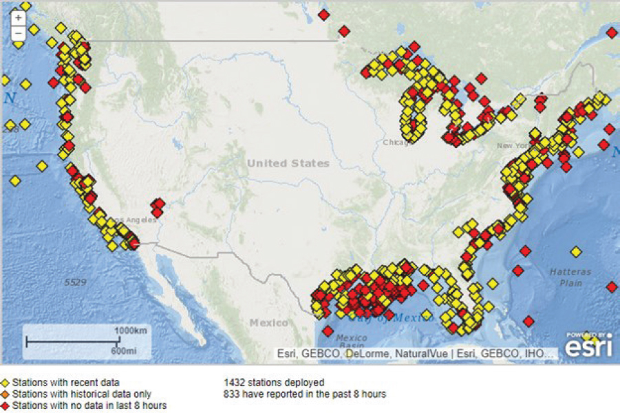
The U.S. National Data Buoy Center (NDBC) provides oceanographic data collected by a network of ocean buoys worldwide¹⁷ (see Figure 4.1). The “active stations file” provides an online list of all 1,432 active stations (buoys, oil rigs, fixed stations, etc.).¹⁸ This file provides metadata on station ID, latitude, longitude, station name, station owner, program to which the station belongs, and type of data reported for all active stations on the NDBC website.

The data elements available for download by station from the NDBC include (NDBC, 2015)

• air temperature,
• conductivity,
• currents,
• salinity,
• sea level pressure,
• water level,
• water temperature,
• waves, and
• winds.

Not all stations collect data on all data elements. Data posted to the NDBC web server are stored in ASCII files that can be downloaded via HTTP. The “Realtime Directory”¹⁹ contains the current (last 45 days) data by station. The “Latest Observation File”²⁰ contains essentially the same data elements; however, instead of having the observations from a single station, the file has the most recent observation (provided that the observation is less than 2 hours old) from all stations hosted on the NDBC website. Because this file has multiple stations, it also contains the position

___________________

¹³ See https://psl.noaa.gov/data/gridded/data.cpc.globaltemp.html.

¹⁴ See https://psl.noaa.gov/data/timeseries.

¹⁵ See https://psl.noaa.gov/data/gridded/data.narr.html#detail.

¹⁶ See https://www.ncdc.noaa.gov/cdo-web/datatools.

¹⁷ See https://www.ndbc.noaa.gov.

¹⁸ See http://www.ndbc.noaa.gov/activestations.xml.

¹⁹ See http://www.ndbc.noaa.gov/data/realtime2.

²⁰ See http://www.ndbc.noaa.gov/data/latest_obs/latest_obs.txt.

information (latitude and longitude) for each station. The file is relatively small, less than 100 kB, and is updated approximately every 5 minutes. Historical data files are available by station.²¹ Some stations are equipped with “BuoyCAM” cameras that provide periodic online photos during daylight hours.²²

The National Hurricane Center’s “Blue Water Mariners” program provides a new, experimental, online graphical ocean conditions forecast for mariners that travel the open ocean (NOAA NHC, 2021). The graphic provides information on current wind and wave heights and 12-hour forecast predictions out to 5 days for preset domains over the tropical North Atlantic, Caribbean, Gulf of Mexico, and tropical eastern North Pacific.²³ The National Hurricane Center also provides online access to daily sea surface temperature (SST) maps²⁴ based on data from the National Climatic Data Center. These maps are based on ship and buoy SST data supplemented with satellite SST retrievals. In addition, the NOAA Climate Prediction Center constructed a monthly 1-degree global SST climatology using these analyses.

Medium-Term Climate Trends and Fluctuations

Medium-term trends in climate due to the early effects of gradual climate change and medium-term climate fluctuations due to El Niño and La Niña events may affect the magnitude, seasonal

___________________

²¹ See http://www.ndbc.noaa.gov/station_history.php?station=XXXXX, where XXXXX is station number.

²² See https://www.ndbc.noaa.gov/buoycams.shtml.

²³ See https://www.nhc.noaa.gov/marine/forecast/enhanced_atlcfull.php.

²⁴ See https://www.nhc.noaa.gov/sst.

distribution, and geographic distribution of coastal recreational fishing effort and catch. Medium- and longer-term fisheries policy and management may need to consider ancillary variables related to climate change, El Niño, and La Niña.

Medium-term trends in climate due to the gradual effects of climate change on temperature and precipitation may affect recreational fishing effort and catch. Through simulation modeling, Dundas and von Haefen (2020) investigated the implications of several Intergovernmental Panel on Climate Change climate change scenarios (representative concentration pathways [RCPs]) for recreational fishing using daily temperature and precipitation projections for 2020–2099 (USBR, 2013) for more than 750 locations in the Atlantic and Gulf Coast regions. They found as follows:

These researchers also note that intraday substitution of fishing activity (i.e., shifting coastal fishing from day to night to avoid extreme daytime heat) is likely to increase as the climate warms.

The U.S. Bureau of Reclamation provides online access to downscaled climate projections for the contiguous United States by location. These data are intended “to provide access to climate and hydrologic projections at spatial and temporal scales relevant to some of the watershed and basin-scale decisions facing water and natural resource managers and planners dealing with climate change.”²⁵

Medium-term fluctuations in climate due to El Niño and La Niña events may also affect recreational fishing effort and catch. El Niño and La Niña are the opposite phases of ENSO, or the El Niño-Southern Oscillation.²⁶ Originating in the tropical Pacific Ocean, ENSO is Earth’s single most influential natural climate pattern. El Niño and La Niña alternately warm and cool large areas of the tropical Pacific—the world’s largest ocean—which significantly influences atmospheric circulation patterns that connect the tropics with the middle latitudes, which in turn modifies the mid-latitude jet streams. By modifying the jet streams, ENSO can affect temperature and precipitation across the United States and other parts of the world. El Niño produces cooler and wetter weather over the U.S. South Atlantic and Gulf regions in the winter, but has little effect on summer weather. In contrast, La Niña produces warmer and dryer weather over the U.S. South Atlantic and Gulf regions in the winter, but like El Niño, has little effect on summer weather. The pattern can shift back and forth irregularly every 2–7 years (i.e., “medium-term” climate fluctuations), and each phase triggers predictable disruptions of temperature, precipitation, and winds.

To the extent that the El Niño and La Niña cycle is correlated with recreational fishing effort or catch, it may be possible to use ENSO data to improve annual and in-season recreational fishery catch and effort forecasts made with recreational fishery projection models. ENSO data may be correlated with recreational fishing catch and effort for two, interrelated reasons: first, ENSO effects

___________________

²⁵ See https://gdo-dcp.ucllnl.org/downscaled_cmip_projections.

²⁶ See https://www.climate.gov/enso.

on temperature, precipitation, and runoff in coastal nursery areas may affect the spatial distribution, migration, and/or abundance of target species (Morley et al., 2018; Pinsky et al., 2013), affecting catch rates; second, ENSO effects on precipitation and wind (and catch rates) may affect the recreational fishing effort of anglers (Dundas and von Haefen, 2020). As with other data types discussed above, the usefulness of ENSO data would depend on the accuracy and precision of the data, the frequency with which the data are collected, and the timeliness with which they are made available.

The NOAA National Weather Service Climate Prediction Center’s North American MultiModel Ensemble climate model (Kirtman et al., 2014) is being used to make ENSO predictions²⁷ and probability forecasts for precipitation, temperature, and SST for North America.²⁸

It can be shown that ENSO has a relationship to the relative frequency of seasonal climate extremes in the United States. The frequencies of these extremes vary by region and by season. The NOAA-PSL has produced an online tool²⁹ that plots the increased or decreased risk of extreme warm/cold (or dry/wet) seasons during an ENSO event. These forecasts, predictions, and risk estimates could be used to drive ENSO variables included in recreational fishing projection/forecasting models.

Economic Conditions

Economic variables, such as fuel prices, per capita GDP, and unemployment, may affect recreational fishing effort. Higher fuel prices increase the cost of recreational fishing trips and may decrease fishing effort. Higher per capita GDP increases household wealth, which may increase fishing trips. Higher unemployment may reduce household income, which may reduce effort for higher-priced modes of recreational fishing, such as charter fishing. On the other hand, higher unemployment and lower household income may increase effort for lower-priced recreational fishing modes, such as shore-based fishing. To the extent that these economic variables are correlated (either positively or negatively) with recreational fishing effort or catch, it may be possible to use such economic data to improve annual and in-season recreational fishery catch and effort forecasts made with recreational fishery projection models. For example, Farmer et al. (2020, p. 14) found that “per capita GDP was a useful predictor for private catch rates, possibly indicating more anglers on the water during years with favorable economic conditions. Fuel price was also a useful predictor.”

As with other variables discussed above, in addition to the degree of correlation between economic data and recreational fishery data, the usefulness of economic data would depend on the accuracy and precision of the data, the frequency with which the data are collected, and the timeliness with which they are made available.

The U.S. Bureau of Economic Analysis (USBEA) provides information on per capita GDP on annual, seasonal, quarterly, and inflation-adjusted (“real”) bases.³⁰ This information is available online in several formats from the Federal Reserve Economic Data portal of the Federal Reserve Bank of St. Louis.³¹ Annual and quarterly per capita GDP data are also available by state³² and by county.³³

___________________

²⁷ See https://www.cpc.ncep.noaa.gov/products/NMME/current/plume.html.

²⁸ See https://www.cpc.ncep.noaa.gov/products/NMME/probindex.shtml.

²⁹ See https://psl.noaa.gov/enso/climaterisks.

³⁰ See https://www.bea.gov/data/gdp/gross-domestic-product.

³¹ See https://fred.stlouisfed.org/series/A939RC0A052NBEA.

³² See https://www.bea.gov/data/gdp/gdp-state.

³³ See https://www.bea.gov/data/gdp/gdp-county-metro-and-other-areas.

The U.S. Energy Information Agency³⁴ provides information on gasoline and diesel fuel prices per gallon on a weekly basis by region of the country.³⁵ The data are available for download in spreadsheet format.

The Current Employment Statistics (CES) program of the U.S. Department of Labor’s Bureau of Labor Statistics³⁶ produces detailed industry estimates of employment, hours, and earnings of workers on payrolls. Each month, CES surveys approximately 144,000 businesses and government agencies, representing approximately 697,000 individual worksites. CES National Estimates produces data for the nation, and CES State and Metro Area produces estimates for all 50 states, the District of Columbia, Puerto Rico, the Virgin Islands, and about 450 metropolitan areas and divisions. Data on current employment, unemployment, and the unemployment rate are available online.³⁷

Fishing Access Infrastructure

Fishing access infrastructure consists of fixed assets that facilitate angler access to recreational fishing opportunities. Fishing access infrastructure may increase recreational fishing effort and catch by lowering the cost to anglers of accessing fishing locations along the coast and in the open ocean. To the extent that recreational fishing effort and catch are correlated with fishing access infrastructure, it may be possible to use infrastructure data to improve annual recreational catch and effort forecasts made with recreational fishery projection models. Infrastructure data may be less useful for improving in-season forecasts, as the quantity and quality of infrastructure rarely change within a season because construction time is usually longer than a fishing season. An exception would be the sudden loss of infrastructure due to a disaster (e.g., hurricane strike) or regulatory change (e.g., closing a boat ramp or bridge for repair or closing a beach because of water quality problems). For example, reductions in beach width have been found to reduce shore fishing effort, although some of that “lost” effort is displaced, for example, to nearby pier or jetty infrastructure (Whitehead et al., 2009). Again, in addition to the degree of correlation between infrastructure and recreational fishery data, the usefulness of infrastructure data would depend on the accuracy and precision of the infrastructure data, the frequency with which the data are collected, and the timeliness with which they are made available.

Fishing access infrastructure may be open to use by the public, such as in the case of boat ramps, fishing piers, bridges, jetties, and beaches, or it may be privately owned, such as in the case of private marinas and boatslips and docks attached to private residences.

The MRIP APAIS program uses data on public infrastructure in developing fishing pressure weights to improve APAIS estimates. MRIP maintains an online database of saltwater fishing access sites that serves as the sample frame for the APAIS of recreational anglers. This Public Fishing Access Site Register³⁸ contains information on more than 3,800 marinas, boat ramps, beaches, and other public fishing access sites along the Atlantic and Gulf Coasts from Maine to Louisiana, including information on infrastructure at each location, such as the number of boat ramps, number of parking spaces, lighting at night, tackle shops, fuel docks, cleaning stations, and nearby restaurants and hotels. For Texas, which is outside of MRIP, an interactive map³⁹ of coastal public boating access locations and amenities is maintained by the Texas General Land Office.⁴⁰

___________________

³⁴ See https://www.eia.gov/petroleum/gasdiesel.

³⁵ See http://www.eia.gov/oil_gas/petroleum/data_publications/wrgp/mogas_history.html.

³⁶ See https://www.bls.gov/ces.

³⁷ See https://www.bls.gov/bls/newsrels.htm#OEUS.

³⁸ See https://www.fisheries.noaa.gov/recreational-fishing-data/public-fishing-access-site-register.

³⁹ See https://cgis.glo.texas.gov/txcoasts.

⁴⁰ See https://www.glo.texas.gov.

In addition to the data on public fishing access infrastructure, data on private infrastructure might also be used to improve recreational effort and catch estimates. Data on private infrastructure are not currently collected by MRIP, but such data could be gleaned from other sources. For example, licenses or permits may be required to construct private docks or boatslips in some areas, and it may be possible to obtain lists of these locations from local permitting agencies. Google Earth could be used to search for private marinas and boatslips, perhaps with the aid of machine learning algorithms to identify relevant infrastructure features. The Google Earth search engine can search for linear features perpendicular to a shoreline (Gorelick et al., 2017), which could help in identifying private docks and piers. Real estate databases, such as the Multiple Listing Service⁴¹ of the National Association of Realtors,⁴² typically include information on the waterfront status of property parcels and whether single-family residence parcels have a boatslip. For duplex, multiplex, condominium, and single-family parcels in a homeowners association, such databases often indicate whether each parcel has an assigned boatslip in a communal dock or marina, access to unassigned boatslip(s) in a communal dock or marina, or no boatslip access.

These data on public and private infrastructure could be used to help explain differences across regions and across years in MRIP output effort and catch results. This might improve estimates of the initial (season-start) conditions for in-season projection models or within-season projections in cases in which new infrastructure is projected to become available within the season (e.g., a new boat ramp will open or repairs will be completed on a fishing pier).

Boat Ownership

Boat ownership may increase recreational saltwater fishing effort by increasing the accessibility of deeper-water fishing areas to anglers. Boat ownership may also increase effort by reducing the cost of a fishing trip by decreasing reliance on more expensive charter boat and headboat fishing modes. Access to alternative deeper-water fishing areas may also increase CPUE in some cases, and increases in CPUE may further increase effort. For example, Gillig et al. (2000) investigated boat ownership as an ancillary variable to explain the number of fishing trips per angler targeting Red Snapper in the Gulf of Mexico in the early 1990s. The researchers found that anglers who own boats take more Red Snapper trips relative to anglers who do not own boats. Therefore, the proportion of anglers that own boats may be a useful ancillary variable for the purpose of forecasting recreational saltwater fishing effort and catch. State recreational fishing vessel ownership registries could be combined with saltwater fishing license registries to determine the proportion of saltwater anglers that own boats, as well as how this proportion varies over time and by geographic region.

Social, Cultural, and Demographic Factors

Fishing effort is influenced by a wide variety of social and cultural factors, some of which may be useful as ancillary variables in effort forecasting models. For example, it is well known that fishing effort varies by the day of the week (weekdays versus weekends) and is affected by holidays (Powers and Anson, 2016). The dates of fishing tournaments and seafood festivals may also affect effort, and the dates of such events are usually available from state resource management agencies. Demographic factors, such as age and ethnicity, may affect fishing effort as well. For example, communities with larger versus smaller proportions of older anglers may have different preferences regarding fishing modes, target species, and trip frequency. As another example, communities with different ethnic backgrounds may celebrate different holidays, with different implications for

___________________

⁴¹ See http://www.mls.com.

⁴² See https://www.nar.realtor.

fishing effort. Demographic data are available at the county level from the U.S. Census Bureau’s Quick Facts data tool.⁴³

Substitute Recreational Activities

The availability of substitute outdoor recreational activities, such as deer hunting and duck hunting (Gentner and Sutton, 2008; Oh et al., 2013; Sutton and Oh, 2015), may also affect recreational fishing effort. The seasonal dates of such activities are available from state resource management agencies. As overlapping management seasons can force choices among substitutable activities, understanding the management of competing activities could potentially improve predictions of fishing effort. However, it is widely known that recreational fishers are heterogeneous in their characteristics and preferences (e.g., avidity and specialization), and this context would influence substitution choices (Oh et al., 2013).

Disaster Events

Disasters such as hurricanes and oil spills can have large, if transitory, effects on recreational fishing effort and catch. Hurricanes can affect recreational fishing effort before, during, and after making landfall. Before landfall, anglers must spend time preparing their boats to weather the storm. During landfall, a period that can last from a few hours to a few days, severe wind and waves reduce fishing effort to zero. Following landfall, anglers must often deal with loss of electrical power, roads blocked by fallen trees, children at home because of school closings, loss of infrastructure, or even damage to boats and homes. To the extent that these hurricane strikes are correlated (either positively or negatively) with recreational fishing effort or catch, it may be possible to use data on hurricane strikes to improve annual and in-season recreational fishery catch and effort forecasts made with recreational fishery projection models. Again, in addition to the degree of correlation between hurricane strikes and recreational fishery data, the usefulness of hurricane strike data would depend on the accuracy and precision of the data, the frequency with which the data are collected, and the timeliness with which they are made available.

Even relatively weak storms can have significant impacts on fishing effort. A recent example from commercial fishing in North Carolina makes the point. Dumas (2021) surveyed the full population of North Carolina commercial fishers (N = 2,496; response rate 22.7 percent, N = 566) in early 2020 regarding fishing activity during 2019. Hurricane Dorian, a Category 1 hurricane, struck North Carolina on September 5–6, 2019 (USNWS, 2019). On average statewide, in addition to missing 2 days of fishing during the actual hurricane strike, survey respondents reported missing five fishing trips before the hurricane strike and an additional nine fishing trips after the hurricane strike because of actions necessary to prepare for and recover from the hurricane.

The U.S. National Hurricane Center produces 5-day and 2-day tropical weather outlooks⁴⁴ that could be used to inform recreational fisheries projection models. Hurricane forecast error methodology and verification procedures⁴⁵ are also available. For pre–fishing season forecasts, historical hurricane data are available with which to develop seasonal probability distributions for hurricane strikes for particular locations. The Atlantic HURDAT2 dataset is available online in a comma-delimited, text format with 6-hourly information on the location, maximum winds, central pressure, and (beginning in 2004) size of all known tropical and subtropical cyclones.⁴⁶

Oil spills may also have significant impacts on recreational fisheries. For example, Tourangeau et al. (2017) and English et al. (2018) report on the effects of the Deepwater Horizon oil spill that

___________________

⁴³ See https://www.census.gov/programs-surveys/sis/resources/data-tools/quickfacts.html.

⁴⁴ See https://www.nhc.noaa.gov/gtwo.php?basin=atlc&fdays=5.

⁴⁵ See https://www.nhc.noaa.gov/verification.

⁴⁶ See https://www.nhc.noaa.gov/data/#hurdat.

occurred on April 20, 2010, 50 miles off the coast of Louisiana on recreational shore-mode fishing in the Gulf of Mexico. During the first 8 months following the spill, there was a 45.5 percent reduction in beach-based recreational fishing trips in the North Gulf region (i.e., Louisiana to Apalachicola, Florida) and a 22.9 percent reduction in such trips along the west coast of Florida. There was also a 32.8 percent reduction in trips to non–beach shore locations (i.e., fishing from piers, bridges, jetties, etc.) in the North Gulf region. In the period from 9 to 18 months following the spill, the number of beach-based recreational fishing trips remained 10.1 percent below the baseline level. Of the trips that did not occur in the North Gulf or west Florida study regions, approximately 39 percent still occurred but were relocated to the coastal areas of Texas and the east coasts of Florida and Georgia. Results from such studies give some indication of the duration and magnitude of the impacts of disasters on recreational fishing effort, including spatial relocation of fishing effort outside the region of immediate impact.

Internet, Cell Phone, and Social Media Activity

Internet, cell phone, and social media activity patterns could provide another source of continuous data on fishing effort in season. For example, in a case study in Scotland, Mancini et al. (2018) investigated the use of photos uploaded to Flickr as an indicator of nature-based recreation on a national scale and at several regional spatial and temporal resolutions. The researchers found that spatial and temporal patterns in photographs of wildlife uploaded on Flickr⁴⁷ are reliably described by known survey measures of visitation and that this relationship is reliable down to a 10-km scale resolution.

Merrill et al. (2020) estimated daily visitation to water recreation areas in New England using commercially available cell phone location data⁴⁸ and ancillary variables. By combining these data with on-the-ground observations of visitation, the authors fitted a model for estimating daily visita-

___________________

⁴⁷Mancini et al. (2018) describe how they accessed and used the Flickr data: “Data from Flickr were collected through the Flickr API (Flickr Services, 2021) and R software], using the packages RCurl version 1.95.4.7, XML version 3.98.1.3 and httr version 1.1.0 to communicate with the API, request and download the data. Dates and geographic coordinates associated with the photographs were used to select only those taken in the [national park] between 2009 and 2014. A bounding box was used to query the Flickr API and then a polygon shapefile of the [national park] was used to select only the photographs taken inside the boundaries of the park. We downloaded the following metadata associated with the photographs: photograph and user ID, the date when the photograph was taken and the geographic coordinates of where it was taken. To avoid bias coming from having a small number of very active users, we used the combination of user ID and date to delete multiple photographs from the same user on the same day, thus retaining only the first photograph taken every day by each user. By counting the number of photographs retained in each month we then obtained the monthly number of Flickr visitor days in the [national park] (a person taking at least one photograph a day in the [national park]). To quantify changes in the popularity of Flickr over the years, we used the number of active users (i.e. users posting content on Flickr).”

⁴⁸Merrill et al. (2020) describe how they accessed and used cell phone data: “We purchased data products processed by a third-party provider, Airsage, Inc. This provider creates population-level estimates of human mobility derived from a panel of over 120 million devices using location information from smartphone applications (see S1 File). The data provider processes this device-specific locational information. Before we receive it, the data is anonymized and aggregated to contain no personally identifiable information. We do not obtain any device-level information, nor raw device GPS locations, but instead, we obtain aggregated summaries of visitation by recreation site and estimates of the visitors’ origin census block-group geographies. The data provider translates their sample to population-level estimates using weights based on the share of the population their sample represents by census-tract geographies. The cellular device sample we purchased data from includes about 30 percent of the U.S. population but varies by tract and month. To obtain the cell data for the sample geographies of interest, we spatially buffered (added area) around the water-access sites which were designated as line or point features in the original spatial databases. In consultation with the data provider and after attempting a range of spatial buffers, a 100-meter buffer was chosen to balance specificity in capturing water recreation visits (i.e., not capturing ancillary points of interest in geographies, like restaurants or stores, for example) with the accuracy of the locational information. We sent the defined water recreation areas to the data provider as a set of geographic extents, or polygons, and they returned the aggregated and anonymized processed data in tabular form. We … include the entirety of this dataset available with the code package associated with this work at https://github.com/USEPA/Recreation_Benefits.git.”

tion for 4 months to more than 500 sites. However, spotty cell phone connectivity in remote areas is one limitation of this method, and spatial autocorrelation and the statistical assumptions made by the providers of cell phone data are issues for further investigation.

A study by social scientists at NOAA’s Southeast Fisheries Science Center explored the potential use of regression-based models of Google Trends to estimate in-season harvest rates in the context of changing fishery conditions (Carter et al., 2015). For instance, Internet search volume for the term “Red Snapper season” was found to be highly correlated with Red Snapper harvest levels. The study also demonstrated that a “nowcasting” model enhanced with Google Trends data was 29 percent more accurate than predictions based on the previous fishing season. The authors argue that such approaches could improve management responsiveness in fisheries, particularly those in which conditions often change.

Remote Sensing

Remote-sensing and satellite technologies have fundamentally changed the way data are collected and used to forecast the weather, study the climate, manage land resources, and monitor many other natural resources. Early connection of satellite remote-sensing data to fishery was made in the 1970s when it was found that lights from fishing boats can be detected with low-light imaging data collected at night by sensors flown on satellites. Nevertheless, remote sensing was not established as a reliable tool for surveying fishing activities until more recently, when advances in satellite technology and data science techniques finally made this possible. The launch of Google Earth Engine⁴⁹ (Gorelick et al., 2017), a cloud computing platform for processing and analyzing global satellite and other geospatial and observation data, had greatly reduced barriers to the use of remote-sensing data. This technology has great potential to provide low-cost auxiliary data that could be used to infer fishing effort and help improve in-season management.

Recent literature has established that three types of remote-sensing data can be used effectively to survey fishing activities. One is Automatic Identification System (AIS) data, the position signal broadcast by ships and picked up by satellite-based receivers. The second is the low-light imaging data collected by the National Aeronautics and Space Administration/NOAA Visible Infrared Imaging Radiometer Suite (VIIRS). Both of these datasets are publicly available and can be downloaded and analyzed for free through the Google Earth Engine. The third type of remote-sensing data, currently under development, is remote sensing of outdoor parking lot utilization (such as parking lots at public-access boating locations).

In a study published in the journal Science (Kroodsma et al., 2018), the authors organized an interdisciplinary team of data scientists, software engineers, ecologists, and economists to design artificial intelligence algorithms that processed 22 billion AIS position signals and turned them into the time and place of fishing activities. The result was a global dynamic footprint of industrial fishing effort with unprecedented spatial and temporal resolution. This methodology is used by the Global Fishing Watch to produce a Daily Fishing Hours dataset, which provides estimates of fishing effort measured in hours of inferred fishing activity. These data are available on the Google Earth Engine and can provide valuable information for local fishery management.

Although AIS data have been shown to be very effective at mapping industrial fishing efforts, the data do have two limitations. One is that AIS typically covers only the larger boats used in industrial fishing, and most of the boats used in recreational fishing will not be detected. Another is that the ship operator can disable or tamper with the AIS to evade detection. VIIRS data can serve as a complementary data source to overcome the limitations of AIS data. Currently VIIRS is on board two satellites, the Suomi NPP, launched in 2011, and the NOAA-20, launched in 2017.

___________________

⁴⁹ See https://earthengine.google.com.

NOAA’s Earth Observation Group produces a nightly global mapping of VIIRS boat detections, which is publicly available online.⁵⁰ The VIIRS Day/Night Band data are available through Google Earth Engine. Several recent publications have established that a combination of AIS and VIIRS data can be used effectively to survey certain fishing activity (see, e.g., Chen et al., 2019; Geronimo et al., 2018; Ruiz et al., 2020).

As satellite, artificial intelligence, and machine learning technologies improve, progress is being made in counting filled and unfilled parking spaces in parking lots for the purposes of forecasting general parking demand and improving the efficiency of consumer parking activity in urban areas and transportation in general (Cisek and Lin, 2017; Glaab, 2017; Lambrides et al., 2018; Zambanini et al., 2020). However, such technology could also be used to detect the parking lot utilization percentage at coastal public-access boating locations via satellite remote sensing for use as an ancillary variable that could be useful for forecasting fishing effort on a timelier basis. The percentage of filled parking spaces at public boat ramps is likely correlated with daily fishing effort and in the near future could be assessed daily (electronically, remotely, and automatically), and the data used to help forecast fishing effort on a daily basis. Glaab (2017) notes: “The developed process for parking area detection is robust and achieved a detection accuracy above 95 percent with respect to parking area capacity in fully-exposed image areas. However, the process is not able to sense parking areas that are hidden by objects like roofs or trees.”

METHODS FOR INTEGRATING MRIP AND SUPPLEMENTAL AND AUXILIARY DATA

MRIP can continue its efforts to identify innovative approaches to data collection and data sharing that will support improvements in in-season management. Included in these innovation efforts is continued work on modeling and statistical integration methods (Allen, 2017; Zhang and Chambers, 2019) that draw on MRIP data streams, supplementary data, and auxiliary data to improve timely forecasting and tracking of both point-in-time and cumulative statistics on recreational catch. This section presents several lines of potential development related to catch forecast modeling using MRIP data and other available data sources.

Small Area Estimation Methods

Small-area estimation (Rao and Molina, 2015) considers the problem of producing reliable estimates of parameters of interest and the associated measures of uncertainty for subpopulations (areas or domains) of a finite population for which samples of inadequate size or no samples are available. An example would be attempting to produce reliable estimates of fish catch for MRIP domains with small sample sizes. Areas (domains) are considered “small” if the sample size for the area is not large enough to yield direct estimates of the variables of interest (means, totals, ratios, etc.) with adequate precision (i.e., sufficiently low PSE).

Direct Estimation Methods

The traditional, “direct” methods for producing estimates for a small area are those based solely on the sample data collected within the small area and perhaps auxiliary data describing the same small area. Direct estimates (Cochran, 1977) are generally design based in the sense that they make use of survey weights, and the associated inferences (e.g., standard errors and confidence intervals) are based on the probability distribution induced by the sample design, with the population values

___________________

⁵⁰ See https://www.ngdc.noaa.gov/eog/viirs/download_boat.html.

held fixed. Although direct methods typically produce unbiased estimates, it is often not possible to achieve a sufficiently large overall sample size to achieve acceptable precision (PSE) for small-area domains of interest. For example, to produce reliable estimates for small areas the size of school districts, a sample of at least one in six households would be required nationwide (Rao and Molina, 2015).

The problem of low precision in small-area domains that is typical for direct estimation methods may be ameliorated somewhat by applying “compromise sample allocation” (Rao and Molina, 2015, Section 2.7). Compromise sample allocation is achieved by oversampling small areas, that is, shifting some of the sample effort from non-small areas to small areas. This can sometimes substantially increase the precision of the estimates for small areas at the cost of a slight decrease in precision for aggregate estimates over the total population. In an example involving the Canadian Labour Force Survey, Singh et al. (1994) found that compromise sample allocation could reduce the coefficient of variation (CV) of the direct estimate of the number of unemployed persons from 17 percent to 9.4 percent for small areas while increasing the CV of the aggregate estimate at the province level from 2.8 percent to only 3.4 percent and the CV of the aggregate estimate at the national level from 1.36 percent to only 1.51 percent.

Indirect Estimation Methods

In cases in which sample size and compromise sample allocation are not sufficient to produce reliable estimates for small areas, “indirect” estimation methods can be used. This approach moves away from design-based or direct estimates to indirect, model-dependent estimates. Other terms for indirect estimation include “nontraditional,” “small-area,” “model-based,” “model-dependent,” and “synthetic” methods. Increasing the precision (reducing the mean squared error [MSE]) of the estimates for small areas beyond what is achievable with direct estimators is the main reason for using indirect estimators. For example, Young (2019) and Cruze et al. (2019) provide an overview of many model-based techniques currently used by the U.S. Department of Agriculture’s National Agricultural Statistics Service (USDA-NASS) (e.g., Cruze and Benecha, 2017). Wang et al. (2012), Nandram et al. (2014), and Cruze (2016) developed model-based approaches for combining multiple sources of survey data with other sources of information, with the aim of improving the USDA-NASS crop forecasting process (NASEM, 2017b). The forecasts precede the publication of end-of-season state estimates, similar to the situation in which in-season forecasts of fish catch are needed for in-season management before the end-of-season final catch estimates are available.

The indirect, model-dependent approach employs a statistical model for a small area that links variables of interest and auxiliary data and/or “borrows strength” from other small areas or other time periods. Regression models, mixed-effect models, and spatiotemporal models are typically used to bring information from auxiliary data and data in related areas (domains) to the estimation process. The availability of good auxiliary data and determination of suitable linking models are crucial to the development of indirect estimates. See, for example, Cruze (2015) and Erciulescu et al. (2019), who present models for integrating survey data with auxiliary sources of information to estimate crop yields, and Wang et al. (2018), who use regression and spatial models to estimate proportions in small areas in the National Resource Inventory survey.

The issues of aggregation over domains and benchmarking are important for indirect estimators (Erciulescu et al., 2018). Aggregation refers to the problem of ensuring that estimates produced at different domain levels (e.g., county, state, and region) are consistent. Benchmarking refers to the problem of ensuring that area-wide estimates are consistent with external, overall estimates (e.g., Bell et al., 2013; Erciulescu et al., 2019; Nandram et al., 2019; Pfeffermann and Barnard, 1991). Solutions to these problems can depend on the type of estimate desired—a numerator, a denominator, and/or their ratio (e.g., fish catch, fishing effort, and catch per effort). Simultaneously

estimating a set of desired statistics (e.g., a numerator, a denominator, and their ratio) is a difficult problem because the final triplet estimates need to satisfy identity constraints (ratio of numerator to denominator) as well as benchmarking constraints at multiple aggregation levels. Erciulescu et al. (2018) explore different methods of constructing model-based estimates for two totals and their ratio at lower-level domains that aggregate to fixed values at upper-level, aggregate domains.

Indirect estimators can be classified by the source of data from which they borrow strength. A domain indirect estimator makes use of y values from another domain but not from another time period. A time indirect estimator uses y values from another time period for the domain of interest but not from another domain. A “domain and time indirect” estimator uses y values from both another domain and another time period.

Indirect estimators can be further categorized as “synthetic,” “composite,” or “James-Stein” (or shrinkage) (Rao and Molina, 2015, Sections 3.2–3.4).

Synthetic Estimators

Synthetic estimators combine a direct estimator that is reliable for the total, aggregate area, with the assumption that the small areas have the same characteristics as the large area, to derive better estimates for the small areas. The Horvitz-Thompson direct estimator is typically used for the large area. Synthetic estimators typically use auxiliary information at the area level or at the individual sample unit level (e.g., Cruze, 2015). (For cases in which the only available auxiliary information is the population area sizes, the broad area ratio estimator can be used.) An example of a synthetic estimator is a regression that estimates the relationship between the variable of interest and auxiliary variables for the non-small areas in a region, which is then used to produce estimates of the variable of interest for small areas in the region. Hansen et al. (1953, pp. 483–486) described the first application of a synthetic regression estimator in the context of a radio listening survey.

Although synthetic estimators may reduce the variance (PSE) of estimates for small areas, they typically produce biased estimates. If the assumption that small areas have the same characteristics as the large area is not fulfilled, for example—if selection effects cause systematic differences in the target variable between a small domain and the population—then synthetic estimators can be heavily biased. Furthermore, for some synthetic estimators, the estimates for small areas do not add up to the direct large-area estimate. In such cases, adjustment is needed to ensure the coherence of estimates at different levels of aggregation.

Composite Estimators

Composite estimators are the weighted average of a direct estimator and a synthetic estimator, sometimes with a different weight for each domain. This estimator is more useful when there is substantial variation in sample sizes across domains. The weight(s) are typically optimized to minimize the MSE of the composite estimator; however, it is often the case that even sizable deviations from the optimal weight do not produce a significant increase in the MSE of the composite estimator. Composite estimators represent an attempt to achieve a balance between the low-precision problem of direct estimators and the bias problem of synthetic estimators. The larger the sample size in the small-area domains, the more weight that should be placed on the direct estimator.

Sample size–dependent (SSD) estimators are composite estimators with simple weights that depend only on the domain counts or the domain totals of an auxiliary variable. General SSD estimators provide consistency when aggregated over different characteristics because the same weight is used for all of them. Unfortunately, general SSD estimators for subdomains do not add up to a direct estimator at a large-area level; however, a simple ratio adjustment can correct this problem. As an example, Statistics Canada now uses the Fuller-Rao method (Fuller and Rao, 2001) for its

official labor force statistics production. Bonnery et al. (2013) found that the Fuller-Rao method outperformed the direct estimation method when applied to U.S. Current Population Survey data on U.S. unemployment rates. Opsomer et al. (2003) provide another example of a regression composite estimator applied to watershed erosion.

James-Stein Estimators

In general, many statistical methods attempt to produce unbiased estimates with the lowest possible variance. For example, in the traditional linear regression statistical model with independent and identically distributed normal errors, the least-squares estimator or the maximum likelihood estimator can be used to produce unbiased estimates with minimum possible variance. “Stein rules” (Judge and Bock, 1983; Judge et al., 1985, Chapter 3; Stein, 1955) are statistical methods that attempt to produce estimates with even lower variance, but at the cost of allowing a bit of bias in the estimates. Given the typically large variance in forecasts of fish catch, fishery managers may be willing to accept a little bias in the catch estimates if the variance (PSE) can be reduced substantially. For example, a fishery manager might be willing to accept 5 percent bias in the catch estimate if the PSE can be reduced from 70 percent to 30 percent.

James and Stein (1961) developed an estimator that, under squared error loss, has lower expected loss for all possible values of the unknown parameters relative to the least-squares estimator. This means that the unbiased least-squares estimator has higher MSE compared with the biased James-Stein estimator. James-Stein estimators are a special case of a composite estimator in which the weights are the same for all small-group domains. This ensures good precision for the group of small areas but not necessarily for individual small areas that have unusually large or small deviations from the mean. However, the estimate of the weight is very reliable because it comes from pooling over small areas. Large gains in precision can be achieved over traditional design-based estimates without assuming a model for the individual small-area parameter weights.

Other estimators similar to, or derived from, the James-Stein estimator have been developed for various applications (Efron and Morris, 1975), including incorporation into Bayesian model frameworks (Efron and Morris, 1973). James-Stein rules used in conjunction with inequality restrictions on the parameters, so-called “positive Stein rules” can achieve MSE even lower than that of the James-Stein rule (Judge and Bock, 1978). Stein rules in general are simply a type of pretest estimator that is used to optimally combine unrestricted and restricted least-squares estimators. (In fact, if some parameter restrictions [equality or inequality restrictions] are known to be true, then the restricted least-squares estimator can produce unbiased estimates with MSE lower than that of simple least squares [Judge et al., 1985, Chapter 3].)

For example, the “Fay-Herriot” method (Fay and Herriot, 1979) is a popular implementation of the James-Stein rule concept. The Fay-Herriot method has been applied to estimate per capita income and poverty in small towns (NRC, 2000) and agricultural crop yield and acreage (Cruze et al., 2019), as well as to calibrate Coastal Household Telephone Survey (CHTS) and FES survey data in MRIP (Papacostas and Foster, 2018, pp. 62–66).

Although James-Stein rules may produce good estimates on average across all observations in the dataset, they may not do so for particular data points, such as outliers. To limit the maximum bias possible for the estimate of any particular data point, Fay and Herriot (1979) use an inequality-restricted form of the James-Stein rule. The inequality restrictions limit the maximum bias while still achieving much of the reduction in MSE. It is important to note that Fay and Herriot (1979) present several other versions of James-Stein rule estimators that are appropriate for various circumstances, including estimators incorporating ancillary variables and estimators that can be integrated

with a Bayesian modeling framework. If fishery managers are willing to accept some amount of bias in catch forecasts, then it may be possible to develop custom, “Stein rule”–like estimators to reduce the variance (PSEs) of catch forecasts and lower the forecasts’ overall MSE.

Small-Area Models

Small-area models are small-area estimation methods that account for differences in variation among areas (domains) beyond those explained by auxiliary variables included in the model. Unlike the global (averaged over small areas) measures of precision produced by synthetic estimators, area-specific measures of precision (PSEs) can be associated with each small-area estimate.

The essence of all small-area methods is the use of auxiliary data available at the small-area level, such as administrative data or data from the last census. These data are used to construct predictor variables for use in a statistical model that can be used to predict the estimate of interest for all small areas. The effectiveness of small-area estimation depends initially on the availability of good predictor variables. One key distinction in small-area models is between situations in which the auxiliary data are available for the individual units in the population and those in which they are available only at the aggregate level for each small area. In the former case, the data can be used in unit-level models, whereas in the latter they can be used only in area-level models. Aggregate-level (or area-level) models are the models that relate small-area direct estimators to area-specific auxiliary variables. Such models are necessary if unit- (or element-) level data are not available. Unit-level models are the models that relate the unit values of a study variable to unit-specific auxiliary variables.

Area-Level Models

Area-level models rely on area-specific auxiliary data and typically assume that the sampling variance in each domain is known and that the model in each domain is the same as the population-level model. The Fay-Herriot (1979) model is an example of an area-level model. Extensions of the Fay-Herriot model address multiple response variables, correlation in sampling errors across areas, and spatial effects. Rao and Yu (1992, 1994) present a Fay-Herriot model based on time-series cross-sectional data. Nandram et al. (2019) present a Fay-Herriot model in a Bayesian framework. The panel that authored a recent National Academies report (NASEM, 2017b) on improving small-area estimates for agricultural variables found that USDA-NASS was pursuing area-level models (Cruze et al., 2016; Erciulescu et al., 2019). In the report, the panel suggests starting with area-level models. It is straightforward to add covariates to such models. The covariates may be added via a simple linear model or via a more flexible form, such as those used in the machine learning literature; it would be best to begin with simple, interpretable models. The panel suggests that USDA-NASS begin by exploring county-level models using the area-level spatial Fay-Herriot model to describe survey measurements. Each alternative data source could be given its own data model, linked to the larger model in a hierarchical Bayesian framework.

Unit-Level Models

Unit-level models rely on unit-specific auxiliary data. A critical assumption for unit-level models is that the sample values within an area obey the assumed population model; that is, sample selection bias is absent.

Bayesian Approaches

There are also now a number of Bayesian approaches, including empirical Bayes (EB) and hierarchical Bayes (HB), which can be used to estimate small-area models and the variability of small-area estimates (e.g., Cruze, 2016; Nandram et al., 2014; Wang et al., 2012). According to the above-referenced National Academies report (NASEM, 2017b) on improving small-area estimates for agricultural variables, the panel believes that the Bayesian approach holds great promise as recent developments have allowed combining design-based estimates with spatiotemporal smoothing models. For example, Mercer et al. (2015) effectively use a spatial Fay-Herriot (1979) model in the context of modeling childhood mortality based on complex survey data. The basic idea is to assume a hierarchical model in which the first stage is taken as the asymptotic distribution of the direct (design-based) estimator.

Software Implementation

Molina and Marhuenda (2020) produced the R software package “sae” for conducting small-area estimation. Small-area estimation procedures are also available in SAS (Mukhopadhyay and McDowell, 2011).

Capture-Recapture Methods

Liu et al. (2017) present the capture-recapture methodology for combining MRIP data with angler smartphone data (in this case, captured by the Texas iSnapper program) to estimate total catch (King and McCrea, 2019). The investigators developed several statistical estimation models in which “all the proposed estimators allow measurement error in the self-reports and do not make any assumptions about their representativeness.” The capture-recapture estimators are compared with one that “makes use only of catch observed in the validation sample but not self-reports of catch” (i.e., MRIP estimates). The authors discuss the assumptions, strengths, and weaknesses of the capture-recapture method, report on simulations conducted to assess the relative strength of the estimators, present the results of an example in which they attempted to estimate the total catch of Red Snapper in 2015 in Texas by recreational anglers in private boats using data from the iSnapper program, and provide recommendations regarding which estimator might be preferred depending on conditions in the fishery. Stokes et al. (2021) discuss three types of nonsampling error (undercoverage, matching error, and lack of independence between APAIS intercept and smartphone reporting rate) that can occur when MRIP data and self-reported data from smartphone apps are used to estimate catch using capture-recapture methods. The researchers estimate the bias in catch estimates from each source of nonsampling error in an application to recreational fisheries in the Gulf of Mexico in 2017.

Multiple-Frame Methods

Multiple-frame survey methods may be of interest when considering the potential use of additional, special-purpose surveys to supplement MRIP in order to reduce the variance and PSEs of catch estimates used for in-season management. The use of multiple-frame methods has been discussed and recommended in previous MRIP reviews (NASEM, 2017, p. 149; NRC, 2006, pp. 9, 63, 64, 67, 81-82, 113-114). In a multiple-frame survey, probability samples are drawn independently from multiple sample frames; usually, the samples are drawn using separate surveys, and the data from the separate surveys are then combined and analyzed together. For example, one survey might be MRIP, and another survey might be Florida’s State Reef Fish Survey (SRFS). Sample frames

may overlap; for example, the MRIP and SRFS sample frames overlap for the domain of Florida reef fish anglers. The union of the sample frames is assumed to cover the finite (angler) population of interest. When a multiple-frame survey uses just two sample frames, it is called a dual-frame survey. FES is a dual-frame survey, using both a list frame of licensed anglers and a secondary list frame based on the U.S. Postal Service address-based frame of households (NASEM, 2017, p. 124). APAIS and FES also have different sampling frames: APAIS is based on a spatiotemporal frame, and FES is based on an address (list) frame. MRIP combines information from the two frames to produce total catch estimates.

Hartley (1962) found that a dual-frame survey can cost far less than a single-frame survey that achieves the same precision. Of more interest in the case of combining MRIP with supplemental surveys, Hartley also found that a dual-frame survey can reduce the variance of estimates of population totals (such as total fish catch) compared with a single-frame survey of the same cost. Others⁵¹ have since extended the Hartley methodology. Hartley applications concentrate on a situation in which one frame completely covers the population of interest but is expensive to sample, while the other frame is cheap to sample but covers the population incompletely. The MRIP survey is generally assumed to cover completely the population of licensed recreational saltwater anglers, while other, special-purpose surveys do not cover the population completely but may give more detailed information on a particular domain, such as Florida reef fish anglers, within the overall population of anglers.

Multiple-frame surveys are becoming more common as surveyors attempt to increase the precision of survey estimates at the least cost, especially for subdomains of the population (Lohr and Rao, 2006). For example Madans et al. (2001) discuss multiple-frame surveys in the context of supplementing information from the U.S. National Health Interview Survey (NHIS). Supplemental surveys may be conducted at the state level and then combined with information from the NHIS for improved estimation at the state level. Andrews et al. (2010, 2013) conducted pilot studies applying multiple-frame methods to fisheries surveys in North Carolina, but did not address the particular issue of variance reduction for the purpose of in-season management.

The example presented in Appendix A, on multiple-frame methods, illustrates how Hartley’s basic dual-frame estimator could be applied to the case of combining existing MRIP survey estimates with a supplemental survey for the purpose of reducing the variance of a catch forecast. Several new methods developed in the recent literature have an advantage over traditional methods. Skinner and Rao (1996) and Lohr and Rao (2006) developed a pseudo-maximum likelihood estimator (PMLE) that can be used to combine complex survey data from two or more sampling frames with high efficiency. One common issue in combining survey data from multiple frames is that the response variables from different surveys are often not identical. Measurement error modeling is a useful approach to integrate such survey data (Park et al., 2017). Another promising new approach

___________________

⁵¹Fuller and Burmeister (1972) and Hartley (1974) found that multiple-frame estimators minimize the variance among the class of linear unbiased estimators of a population total, such as the total catch of a population of anglers. Cochran (1964) compared the variance of multiple-frame estimators with that of screening estimators having the same total sampling cost. Rao (2003) examined the uses of multiple-frame surveys for small-area estimation, where a sample from an area frame may be supplemented by less-expensive samples from list frames. Bankier (1986) and Kalton and Anderson (1986) developed single-frame estimators in which observations are weighted according to their inclusion probabilities for the two frames. Skinner (1991) proposed raking ratio estimators for the situation in which simple random samples are taken from each frame, and Skinner and Rao (1996) derived a pseudo-maximum likelihood estimator (PMLE) for the response variable for dual-frame surveys using complex designs. Lohr and Rao (2000) compared the asymptotic efficiencies of dual-frame estimators and found that the PMLE combined high efficiency with applicability to complex surveys. Lohr and Rao (2006) extended the PMLE of Skinner and Rao (1996) to the case of more than two sample frames and conducted a simulation study to explore the finite-sample properties of alternative estimators for simulated two-frame and three-frame designs; they found that “the PMLE is a good choice for a wide variety of conditions.”

for combining data from multiple independent surveys is model-assisted imputation, in which a working model is built at the unit level to generate estimates of variables of interest in survey A using auxiliary variables in survey B (Kim and Rao, 2012). A projection estimator can be constructed by applying the survey weights in survey B to the synthetic value, which is asymptotically unbiased under certain general conditions. Combining multiple-frame surveys is not a trivial task. The effectiveness of this approach depends on the coverage and sample size of the supplemental surveys, the correlation of variables in different surveys, and the magnitude of the measurement error. One also needs to consider the cost of building models to connect multiple surveys in addition to the cost of supplemental surveys when planning for a multiple-frame approach.

Statistical Data Integration for In-Season Management: Integrating Data from Multiple Sources

Collecting probability-based sample survey data such as MRIP and supplemental fishery survey data is expensive, and survey-based estimates alone are unlikely to meet all of the data needs of in-season management under current budgetary constraints. Statistical data integration is an active research area that provides tools for combining MRIP and supplemental fishery survey data with nonprobability survey data for valid statistical inference. The challenge is to overcome the small sample size in survey data sources and the selection bias and undercoverage in big data sources to produce estimates that are asymptotically unbiased with high precision. Lohr and Raghunathan (2017) performed an early review and identified some limitations of the existing methods at that time. Kim et al. (2018) developed a hierarchical multilevel model for integrating survey data, administrative records, and remote-sensing data to improve subarea estimates of planted acreages for different crops. Chen et al. (2020) developed a general framework for constructing doubly robust estimates based on nonprobability sample data and auxiliary data from a probability survey sample. Kim and Tam (2021) developed a two-step regression-based data integration method for the Australian Agricultural Census that can handle the measurement errors in both probability samples and big data sources. Rao (2021) gives an up-to-date overview in this area and provides more detailed discussion of the application to small-area estimation. These recently developed methodologies can be applicable to integrating recreational fishery data for in-season management.

Model-Based Projection/Forecasting or Nowcasting Approaches

Statistical models for forecasting, or projecting, fish catch with a timely frequency are critical for fisheries management (Farmer and Froeschke, 2015; Makridakis et al., 2008; Stergiou and Christou, 1996), especially under an ACL (Farmer et al., 2020; Lee et al., 2017). Catch per time period must be forecast before the season begins so that total, cumulative catch can be forecast and the appropriate season length to meet the ACL determined. In cases in which it is desirable to hold season length constant, catch forecasts are still necessary to determine what changes in other management tools, such as bag or size limits, may be necessary to meet the ACL under a fixed season length. Forecasts are also necessary for applying in-season or post-season AMs, including predicting closure dates. Forecasts are useful as well for establishing a “status quo” catch and estimating the catch under alternative management scenarios when comparing the potential biological and socioeconomic impacts of alternative management actions.

This section briefly reviews existing forecasting methods that have been applied to catch forecasting in fisheries management and describes some potential new methods. The discussion focuses on methods that could be used to improve the accuracy and precision of catch forecasts based on MRIP catch estimate data, perhaps integrated with additional data from supplemental surveys and

ancillary variables. The methods assume that the MRIP catch estimates will be produced using the existing MRIP methodology, or perhaps with modifications to the methodology that would support more frequent MRIP catch estimates (e.g., perhaps monthly or weekly rather than the current bi-monthly estimates). However, modifications to the existing MRIP methodology would likely require technological innovations or additional funding (i.e., increased sampling). When combined with supplemental or ancillary data, some of the methods described in this section may also be useful for increasing the timeliness and frequency of in-season catch forecasts using the current MRIP methodology.

As an example of an existing forecasting model, Lee et al. (2017) developed a bioeconomic model for forecasting recreational catch of cod and haddock in the Northeast region that integrates a model of angler demand for recreational fishing trips with an age-structured stock dynamics model. The model has been in use since 2012. The model combines past MRIP estimates, stock assessment results, and a model of angler trip behavior to project catch, discards, and the effects of recreational removals on the fish stock. The model can make forecasts by month and can project out 3–4 years. The model relies heavily on in-season MRIP data, but the high PSEs (low precision) of MRIP estimates limit their usefulness; furthermore, as waves progress within a season, the PSEs increase. The model is especially useful for forecasting the impacts of alternative management policies (e.g., size limits and possession limits) and fishery parameters (e.g., discard mortality rates and fish length distributions) on recreational catch and discards. Although there are several directions for potential model improvement (allowing anglers to reallocate or shift trips across waves, incorporating information on weather and general economic conditions, considering contemporaneous correlation, etc.), this model is a good example of how a forecasting model using MRIP data can contribute to fishery management under ACLs.

Leveraging Covariances and Conditionals Across Domains

MRIP provides estimates of fish catch and its variance by domain, where a domain is defined as a particular combination of fish species, 2-month wave time period, geographic state or substate location, fishing area (inshore, state ocean waters, or federal ocean waters), and fishing mode (private boat, shore-based, charter, or headboat). Typically, information from only one domain is used by fishery managers to forecast catch for that domain. This approach neglects information in patterns that may exist in the data across domains that might be useful for increasing the precision (decreasing the PSEs) of catch and effort forecasts, such as those made for the purpose of in-season management by fishery managers using the MRIP output estimates.

When fish catch in one domain moves together with fish catch in another domain, the covariance between the two fish catches is positive. When the catches move in opposite directions, the covariance between the two catches is negative. The focus here is not on covariances due to sampling errors in the MRIP survey sampling methodology, but on covariances that reflect the true, underlying relationships among the variables (catches) being estimated by MRIP. In other words, assuming that MRIP perfectly measures catch and that each MRIP estimate is statistically independent (as intended) of every other MRIP estimate, some catches would covary because they were being driven by the same underlying variables.⁵²

___________________

⁵² In a simple linear regression forecasting model context, suppose one regresses the time series of Spanish Mackerel catch on the time series of King Mackerel catch. Suppose (as intended) that MRIP produces a time series of statistically independent estimates of the catch of each species at each point in time. Then, while the (autocorrelation-adjusted) errors in the regression model would be independently (and for the sake of discussion identically) distributed, the estimated regression coefficient would likely be positive, because the catches of Spanish and King Mackerel tend to move up and down together. The discussion here is concerned with the regression coefficient as an indicator of correlation, and hence covariance, between the catches rather than with the MRIP sampling program that produced the catch estimates.

For example, one might expect that the covariance between the catch of two species in a particular location that prefer the same water temperatures would be positive because when the water is warm, both species would be more abundant in that location and catches of both would be higher, whereas when temperatures are low, both species would be less abundant and catches of both would be lower.⁵³ Inversely, one might expect that the covariance between the catch of two species that prefer different water temperatures would be negative.

As another example, the catches of predator and prey species might have a negative covariance (high predator concentrations result in low prey concentrations, and low predator concentrations result in high prey concentrations). Or, if increases in the Dolphin population led to increased Dolphin catches in both the charter boat and private boat fisheries, and decreases in the Dolphin population led to decreased catches in both fisheries, then the covariance in Dolphin catch between the two fisheries would be positive. As yet another example, if the Dolphin population increased off the coasts of both North Carolina and South Carolina, one might expect the Dolphin catch in both states to increase, and one would expect the covariance to be positive between the North Carolina Dolphin and South Carolina Dolphin catches.

The covariance in catch across MRIP domains is likely not zero for many domain combinations. The reason behind this observation is that MRIP produces a catch estimate for each domain by multiplying an estimate of fishing effort (i.e., fishing trips) for the domain by an estimate of the catch per unit effort (i.e., catch per fishing trip), or CPUE, for the domain. The estimates are weighted such that the effort estimate is statistically independent of the CPUE estimate within a domain. However, the effort in one domain may be correlated with the effort in another domain, not because of any problems with the MRIP sampling or estimation methodology but simply because the true efforts are actually moving in the same direction.

For example, if anglers increased trips to two fishing areas over time, then the effort in both areas would increase together—the efforts in the two areas would be correlated over time and not independent. MRIP would produce statistically independent estimates of each effort data point, but the actual effort variables themselves would not be independent, either because there was a true causal relationship between the variables or because there was a third “driver” variable influencing both effort variables. Similarly, CPUE in one domain may not be independent of CPUE in another. For example, suppose that warm seawater temperatures increased the local abundance of two different fish species in a given area, then the CPUE for both species (both domains) would increase together—the CPUEs would be correlated across species and not independent.

Finally, effort is likely not independent of CPUE across locations or time periods. For example, Gillig et al. (2000) investigated the effect of Red Snapper CPUE (from the MRFSS) on fishing effort (trips per angler) targeting Red Snapper for reef fish anglers in the Gulf of Mexico in 1991. The researchers conducted a cross-sectional study and found that CPUE was correlated with fishing effort. This implies that the covariance between fishing effort and CPUE across locations is not zero. Similarly, the covariance between fishing effort and CPUE across time periods is likely not zero. Fish length and the length distributions of fish catch may also be correlated by fishing location, time period or fishing mode; for example, Lee et al. (2017) note: “If fish aggregate by size then the lengths of fish caught on a trip are likely to be positively correlated.… Human behavior, such as angler skill or targeting, could also produce positive or negative correlations between [catch] numbers and length within and across species.”

Appendix B, on Leveraging Covariances and Conditionals, provides examples of some methods that use covariances between domains and the concepts of conditional expectations and

___________________

⁵³ As another example of potential correlation in catches across species, Lee et al. (2017) note: “If cod and haddock are co-located in the ocean, then the number of cod caught on a trip is likely to be positively correlated with the number of haddock caught on that trip.”

conditional variances to improve catch forecasts made by fishery managers. The first section of Appendix B describes how the covariance in catches across domains depends on the covariance of effort (trips) and the covariance of CPUE across domains. The second section describes how conditional expectations and conditional variances might be used to decrease the variance (PSE) of catch forecasts made by fishery managers. The third section describes how covariances, conditional expectations, and catch information across domains and such auxiliary variables as wind speed, water temperature, or fuel prices could be used to improve catch forecasts and reduce their variance. The fourth section points out the important role of covariances when fishery managers choose to aggregate or disaggregate MRIP catch estimates across domains after receiving the catch estimates from MRIP, with a subsequent note on why covariances among catches in a multispecies fishery constrained by a binding ACL will likely be negative. The final section of Appendix B describes how covariances could be used together with the methodology for using control variates to reduce the variance of catch forecasts.

Despite the possibility of improving catch forecasts through the use of auxiliary variables and forecasting models, these methods may not lead to significant forecast improvements in some situations. For example, the Oregon Department of Fish and Wildlife (ODFW, 2012) found that Yelloweye Rockfish, a rare species with highly variable catch that often reaches its ACL before the catch limits of other non-overfished Groundfish species:

Thus, the applicability of these methods will likely need to be evaluated on a fishery-by-fishery basis, or perhaps for categories of fisheries that share similar characteristics.

Spatiotemporal Models

Spatiotemporal statistical projection/forecasting models attempt to explain the values of one or more dependent variables (such as catch of one or more fish species) based on past values of the dependent variables, and perhaps based on the current and past values of other, independent ancillary variables (such as estimates of stock abundance, season, weather, fuel prices, or the catch of other species) (Hanson et al., 2006). In doing so, spatiotemporal models make use of covariance relationships and conditional relationships among variables, as discussed in the previous section; in this sense, spatiotemporal models can be considered extensions of the concepts discussed in the previous section.

MRIP provides estimates of catch and the variance (PSE) of catch by species. In addition, for each species, MRIP provides these estimates by geographic location, fishing mode, fishing area, and time period. Spatial models attempt to explain the differences in MRIP catch estimates across geographic locations (i.e., across “space”), fishing modes, or fishing areas; temporal models attempt to explain the differences in MRIP catch estimates across time periods (i.e., across time). Spatiotemporal models attempt to explain differences in MRIP catch estimates across both space and time.

From the perspective of constructing projection/forecasting models of fish catch, fishery managers are very fortunate to have the MRIP estimates of fish catch and the variance of fish catch

by species and for different geographic locations and time periods. The MRIP estimates provide a wealth of information that can be used, likely in combination with data on supplementary and ancillary variables, to construct projection/forecasting models of annual catch and catch by 2-month wave. Farmer and Froeschke (2015) found that “federal projection assumptions have been refined over time to better account for changes in average weights and daily catch rates. These refinements have led to increasingly more accurate predictions” (NMFS-SERO, 2013, 2014, 2015, 2016).

Better forecasting models can lead to more opportunities for anglers. For example, because of the accuracy of the federal for-hire forecasts for Red Snapper in the Gulf, the Gulf Council recently reset the component ACT buffer for the federal for-hire component of the Red Snapper fishery from 20 percent to 9 percent below the federal for-hire component ACL, allowing a greater harvest while meeting the ACL (GMFMC, 2019). Where data are sufficient, it may be possible to develop models that produce catch estimates for more frequent time periods, such as by month or week. Good (accurate and precise) projection/forecasting models that produce timely and high-frequency forecasts are needed for in-season management.

Cross-Sectional (Spatial) Models and Spatial Heteroskedasticity

Cross-sectional models are spatial regression models that attempt to explain the variation in catch of a given species across different geographic locations, in a given fishery (fishing mode), for a given time period. Each observation in the model is fish catch at a different location, where all of the catches occur during the same time period. Supplementary and ancillary variables can be used as explanatory variables in an attempt to determine the factors that cause the catch of a given species in a given fishery to differ across locations at a given time. These models make use of MRIP estimates of mean catch and the variance in catch at different locations for a given species in a given fishery at a given time period. The MRIP estimates of the means and variances of catch for a particular species in a particular time period usually differ by location. These models typically exhibit “spatial heteroskedasticity”—the variance in catch differs across geographic locations at a given point in time (Judge et al., 1985, Chapter 11). In cross-sectional models that account for heteroskedasticity, the variance of catch is allowed to vary across locations, but the variance in one location is independent of the variance in another (in contrast to the spatial autocorrelation and seemingly unrelated regression (SUR) models discussed below, in which the variances are not independent across locations).

If catch projection/forecasting models do not account for heteroskedasticity, then although estimates of the forecast model parameters will be unbiased, estimates of the variance (and thus standard errors) of the parameters will be biased, and the direction of bias will be uncertain. Furthermore, the estimate of the variance (PSE) of the catch forecast itself will be biased and the direction of bias uncertain.

Time-Series (Temporal) Models and Temporal Heteroskedasticity

Time-series models are temporal regression models that attempt to explain the variation in catch of a given species across multiple time periods, in a given fishery (fishing mode), at a given geographic location. Each observation in the model is fish catch at a different time period, where all of the catches occur at the same location. These models make use of MRIP estimates of mean catch and the variance in catch across different time periods for a given species in a given fishery at a given geographic location. The MRIP estimates of the means and variances of catch differ across the different time periods. Supplementary and ancillary variables are used as explanatory variables in an attempt to determine the factors that cause the catch of a given species in a given fishery to differ across time periods at a given location. These models typically exhibit “tempo-

ral heteroskedasticity”—the MRIP estimates of the variance in catch differ across time periods (Judge et al., 1985, Chapter 11). In time-series models with heteroskedasticity, the variance of catch is allowed to vary across time periods, but the variance in one time period is independent of the variance in another (in contrast to the temporal autocorrelation models discussed below, in which the variances across time periods are not independent).

Again, if catch projection/forecasting models do not account for heteroskedasticity, then although estimates of the forecast model parameters will be unbiased, estimates of the variance (and thus standard errors) of the parameters will be biased, and the direction of bias will be uncertain. Furthermore, the estimate of the variance (PSE) of the catch forecast itself will be biased and the direction of bias uncertain.

Temporal Autocorrelation Models

Temporal autocorrelation models (Judge et al., 1985, Chapters 7–10), also called “autoregressive” or “moving-average” models, are time-series models in which the dependent variable in the current time period in a particular location (say, the catch of a particular fish species in the current time period in a particular location) may be affected by past values of the dependent variable in that location (past catches of the species in the location). In this situation, the effects of an unexpected “shock to the system” in one time period may linger for subsequent time periods, affecting catch in subsequent time periods. For example, the effects of unexpectedly good recruitment in one year might be observed in several subsequent years. Similarly, the negative effects of an unexpected hurricane strike on effort and catch might linger for several 2-month-wave time periods. Temporal autocorrelation models estimate the magnitude of such lingering effects and estimate how long the effects might persist.

If autocorrelation is present between MRIP estimates of catch (across either years or waves), then although the estimates of forecast model parameters will be unbiased, estimates of the variance (and thus standard errors) of the model parameters will be biased, typically downward, which means that fishery managers are more likely to conclude that a variable in the model has a statistically significant effect on catch when in fact it does not. Furthermore, if autocorrelation is present, the variance (PSE) of a catch forecast made using the model will typically be biased downward. If the variance is biased downward, then the PSE of the catch forecast is underestimated.

MRIP catch estimates are derived from APAIS estimates of catch per trip and FES estimates of trips. Autocorrelation across time in APAIS estimates of catch per trip for a particular species could be caused by variable recruitment, for example, which leads to a recruitment “pulse” flowing through the fish population over succeeding years. (Negative autocorrelation could also occur within a season, as high catch per trip early in the season could reduce the target population, leading to low catch per trip later in the season.) Autocorrelation could also occur across time for FES trip estimates. For example, if trips depend, in part, on the level of unemployment or fuel prices (or on catch per trip, and catch per trip is autocorrelated across years because of recruitment pulses), and the level of unemployment or fuel prices are themselves autocorrelated (which they often are), then the autocorrelation in unemployment, fuel prices, etc. will induce autocorrelation in trips. Autocorrelation in either trips or catch per trip will likely induce autocorrelation in catch.

A time-series model of catch will almost certainly include the values of catch from previous time periods (“lagged” values of catch) as explanatory variables. That is, the model will include lagged values of the dependent variable among the explanatory variables. Such models are called “autoregressive” or AR models (Judge et al., 1985, Chapters 7 and 8). For such models, the covariances between catches from different time periods are nonzero and are important (yet another reason why covariances are important). Durbin’s h test (Durbin, 1970), among others, can be used to test for autocorrelation in a model with lagged values of the dependent variable.

In addition, the current value of catch may be affected not only by random effects (random errors) in the current time period but also by the lingering effects of random errors from previous time periods. Time-series models that capture the lingering effects of random errors are called “moving-average” or MA models (Judge et al., 1985, Chapters 7 and 8).

Time-series models of fish catch would likely include both autoregressive and moving-average effects; such models are called ARMA models (Ives et al., 2010). ARMA models are often “nonstationary”; that is, the variance in catch may explode over time (especially if the fish stock is rebuilding), or the covariance pattern between catches from different time periods may change over time. If the catch data are nonstationary, they may need to be “differenced” to achieve stationarity before further analysis. ARMA models using differenced data that render the data stationary are said to be “integrated,” and so such models are termed ARIMA models (Box and Jenkins, 1976; Judge et al., 1985, Chapters 7 and 8).

Furthermore, looking at MRIP catch estimates over time will almost certainly reveal seasonal patterns, which implies autocorrelation between seasons as well as across years. In the case of seasonal patterns, differencing the data by season or by month may also be required to achieve stationarity (Box et al., 2013). ARIMA models that include differencing by season are known as “seasonal ARIMA” or SARIMA models (Judge et al., 1985, Chapters 7 and 8).

Farmer and Froeschke (2015) compared generalized linear models (GLMs), generalized additive models (GAMs), and seasonal autoregressive integrated moving-average (SARIMA) models in terms of fit, accuracy, and ability to forecast landings of four representative fish stocks that support recreational fisheries in the southeastern United States. These investigators found that “the GAMs provided the best fit to the observed data; however, the modeling approaches of the SARIMA model and GLM provided the best forecasts for most scenarios. The SARIMA model and GLM also provided the best predictions of the seasonal trend in landings, a desirable feature for in-season quota monitoring.” Although, “no single model is likely to perform best for all stocks of interest,” the researchers found that

Not surprisingly, the researchers found that “the time span of input data affected forecast accuracy from all model types considered.” One drawback of SARIMA models is that they “can sometimes generate negative catch forecasts,” in which case the SARIMA models “are likely overfitting a recent trend [in catch].” Simulation studies were conducted to compare several different methods of addressing this drawback, and the conclusions were that replacing the negative catch values with the catch values from the most recent year of fishing “improved forecast accuracy over replacement with zero values in most cases…. In summary, post hoc replacement of negative SARIMA model values with landings from the most recent year of fishing is recommended.”

Farmer et al. (2020) present a case study of using SARIMA methods to forecast Gulf Red Snapper catch in federal waters under an ACL. The purpose of the study was to use SARIMA methods to better estimate catches so that season lengths could be set to maximize fishing opportunities while maintaining catch below the ACL. Specifically, the objectives of the study were to

The investigators identified “the best-fitting model with meaningful covariates for each state and component combination, evaluated the retrospective performance of the forecasting method, and applied our forecasts to predict the 2017 federal season.” Importantly, MRIP estimates of mean catch and the variance of catch were used to identify the best model and to make catch forecasts using the model.⁵⁴ This provides a workable example of how MRIP estimates can be incorporated into a catch forecasting model. The investigators note that “improvements upon this approach may explicitly incorporate the behavioral response of anglers into landings forecasts” (Lee et al., 2017).

Another characteristic of catch data over time is that the effect of an ancillary variable on catch, say, the effect of a “temperature shock” (where temperature is an ancillary variable in the model) on an inshore fish stock, may linger over time. Time-series models that include lingering effects of ancillary variables are called “distributed lag models” (Judge et al., 1985, Chapters 9 and 10). In distributed lag models, a system of weights on the ancillary variables rather than differencing may be preferred for analyzing seasonal data (Pesando, 1972). In addition to the Farmer and Froeschke (2015) models, an example of a relatively simple, yet general, time-series model that incorporates both autoregressive effects (the effects of past catch on current catch) and distributed lag effects (the effects of both current and past values of ancillary variables on current catch) is that of Hendry and Richard (1983); this model includes quite a few other, common time-series models as special cases.

Spatial Autocorrelation Models

Spatial autocorrelation models are cross-sectional models that allow the error in one location to “ripple out” and affect the error in other locations. The purpose of this is to allow the effects of an unexpected “shock to the system” to spread across locations. For example, the effects of unexpected rain might decrease catch in the rainy location but increase catch in nearby sunny “substitute” locations. Spatial autocorrelation models estimate the magnitude of the ripple effect and estimate how far it actually reaches. Unfortunately, spatial autocorrelation models typically require distance data on a relatively fine scale, calculated from GPS coordinates or using a GIS database together with georeferenced locations, and such data are not currently available for saltwater angler fishing locations. As a result, the present study will instead address the issue of spatial correlation by considering contemporaneous correlation of catch between larger geographic regions (e.g., states) or fishing areas (e.g., inshore, nearshore, offshore) within a SUR framework (see discussion below). In the future, alternative data collection methods, such as smartphone apps, may permit the collection of the fine-scale data necessary for spatial autocorrelation models.

___________________

⁵⁴ Specifically, “Parametric bootstrapping techniques were used to directly incorporate variance estimates from the surveys into the projection framework for all projections. The selected linear model function for each state and mode was iteratively fit to 1000 bootstrapped samples of input data for that state and mode based on the mean and variance for those observations. Bootstrapping treated annual catch and weight data as truncated normal distributions with a minimum of zero and a mean and standard deviation from each sampling data source. Regression outputs included the mean and standard error for predicted mean weights and catch rates by state and mode” (Farmer et al., 2020).

Time-Series Cross-Sectional Models

Time-series cross-sectional models (Judge et al., 1985, Chapter 13) combine data on multiple locations and multiple time periods. The dependent variable (e.g., catch of a particular species) depends on the location, the time period, and any other ancillary variables included in the model (e.g., fishing mode, weather, fuel prices). These models may include heteroskedasticity, autocorrelation, or spatial correlation. Engle (1982) presents the classic autoregressive conditional heteroscedasticity model in which both heteroskedasticity and autocorrelation (but not spatial autocorrelation) are allowed; that is, the variance in catch is different for each location, and the variance in catch at a particular location is allowed to vary over time depending on past values of catch at the location. Blanc and Schlenker (2017) provide a discussion of panel data models, a type of time-series cross-sectional model that can be developed when data are available on the same cross-sectional units at each point in time, as opposed to a sample of (possibly different) cross-sectional units at each point in time. The collection of panel data on recreational anglers has been discussed in previous MRIP reviews (NRC, 2006, p. 82) “to gather angler trend data and to improve the efficiency of data collection.”

Contemporaneous Correlation Across Domains (SUR Models)

Typically, information on only one fish species is used to forecast catch for that species. This approach neglects information in patterns that may appear in the data across species (or across other MRIP domains, such as fishing modes) that might be useful for increasing the efficiency (decreasing the PSEs) of catch and effort forecasts necessary for in-season management.

In particular, patterns might exist in the errors of the estimates across domains, such as across fish species or fishing modes. For example, suppose an unforeseen weather event (e.g., a hurricane) that is not in the catch forecast models for two species of fish affects the catch of both species, causing an unexpected decrease in catch for both species. The forecast model for each species would overestimate the catch of its respective species in the year that the hurricane occurred. Both models would forecast catch above the actual catch for the hurricane year; there is a pattern—the forecast catch is above the actual catch for both models at the same time. Both models erred in the same way, at the same time: both had an error in the same direction at the same time; that is, the errors in both moved together, and those errors are said to be contemporaneously correlated.

The SUR method (Zellner, 1962) may in some cases provide a way to improve the efficiency (decrease the PSEs) of catch forecasts made by fishery managers using MRIP output estimates of mean catch, variance (PSE) of catch, and covariance of catches across domains. The purpose of SUR estimation is to make use of contemporaneous correlation in the errors across models (across domains) to improve the efficiency (decrease the PSEs) of forecasts produced by each model (for each domain). The method is called “seemingly unrelated regression” because in some versions of these models, the model equations have no variables in common; the models are related only by their contemporaneously correlated error terms. There appears to be no connection between the models because they have no variables in common, yet they are related through their contemporaneously correlated error terms.

Appendix C, on contemporaneous correlation SUR models, presents the classic SUR model and several extensions. SUR methods are likely to be most useful in situations in which the contemporaneous correlations in errors across equations (across domains) are large. If the SUR method is extended further to allow the errors in one time period in one domain to depend on the errors in all other domains in previous time periods, the vector autoregressive (VAR) model results.

Bayesian Models

Bayesian modeling methods (Doll and Jacquemin, 2018; Punt and Hilborn, 1997; Staton and Catalano, 2019) could be used with MRIP data and/or complementary data (e.g., from state data collection programs) to update catch estimates for the purpose of in-season management of recreational fisheries with ACLs. For example, a Bayesian model that uses MRIP mean catch and PSE estimates to parameterize prior probability distributions and then uses MRIP mean catch and PSE estimates by wave to update priors could provide a method for optimally updating catch estimates and forecasts, setting season lengths, and determining dates of season closures.

From the perspective of the single-species in-season recreational fishery manager, the biological state of the fishery is summarized by the ACL (from a fishery modeler’s perspective, the ACL is the key biological state variable that is fixed within a fishing season but may vary from season to season). The ACL summarizes the best available science regarding the biology of the fishery and the quantity (numbers or pounds) of fish that may be harvested within a season while maintaining the biological integrity of the stock and avoiding such legal thresholds as overfished and overfishing conditions. A second, important state variable that is typically fixed within a fishing season but may vary from season to season is the set of fishery regulations (other than season length) in place at the beginning of the season. For example, traditional fishery regulations that are typically held fixed within a season include size limits, bag limits, trip limits, gear restrictions, etc. Other, “alternative” fishery regulations that may be implemented in the future (but that would likely be held fixed within a season) include harvest tags, recreational registration/stamps, depth/distance-based management, harvest rate/recruitment-based management, a “reef fish” (multispecies aggregate) season, and barotrauma reduction device requirements, among others (GAFGI, 2017; Haddad, 2017). Alternative fishery regulations are discussed in greater depth elsewhere in this report, but for the purposes of the present discussion, the set of all traditional and any alternative fishery regulations in place at the beginning of the fishing season is assumed to remain fixed for the season (but may vary from season to season), and this set of regulations describes the “regulatory state” of the fishery for the season.

Given the initial state of the fishery’s biology for the season, as embodied in the ACL, and given the state of fishery regulations in place for the season, the present discussion focuses on the management problems of (1) setting the fishing season length and (2) determining whether and when to close the fishing season to achieve a desired level of risk, as measured by the probability of exceeding the ACL. This focus appears appropriate given the committee’s Statement of Task (see Box 1.1 in Chapter 1) and recent research indicating the importance and value of fishing season length and predictability to recreational anglers (e.g., Young et al., 2020). The apparent importance to anglers of longer and more predictable fishing seasons implies a management need to maximize the length and predictability of fishing seasons while meeting biological and regulatory constraints. This management task is made more difficult by the many uncertainties inherent in fishery management: uncertainty in the level of angler effort/trips; CPUE uncertainty; weather uncertainty; economic uncertainty (e.g., fuel costs and unemployment rate); and biological uncertainties within the season, including target species location and density, which can be affected by such variables as prey and predator distributions and ocean conditions (e.g., temperatures and currents).

Although many uncertainties exist for in-season fishery management under ACLs, uncertainty can often be reduced over time through learning, leading to better management outcomes. The traditional approach to modeling learning in a management context is to introduce a statistical probability distribution, known as a “Bayesian prior,” that characterizes the manager’s beliefs about the possible values of uncertain model components (LaRiviere et al., 2018). Uncertainty can be reduced over time as managers receive new data (e.g., from MRIP or supplementary state programs), and these data are used to update managers’ beliefs about uncertain model components and improve management decisions through a statistical process known as “Bayesian updating.” This Bayesian

approach (DeGroot, 1970, 1980; Hey, 1985) is adopted and applied here for optimizing the use of MRIP data (and potentially other data, such as those from state programs) for in-season fishery management under ACLs.

The Bayesian approach has several advantages, including the ability to make use of either MRIP data alone, supplementary (e.g., state survey) data alone, or a combination of the two. Furthermore, the approach can be used to measure the incremental management value of adding supplemental data to MRIP data, or vice versa. The Bayesian approach can be used to measure the value of additional information, such as the value of collecting MRIP data more frequently, or the value of adding other, ancillary data, such as weather, economic, or remote-sensing data, to existing data streams (e.g., Lazar et al., 2008; Staton and Catalano, 2019; Wieand, 2008). In addition, the approach can be used to measure the value of disaggregating or segmenting management areas into smaller, more targeted management zones. For data-poor species, the approach can be used to measure the value of implementing new data collection programs. Because of space limitations, not all of these potential applications can be examined in detail here. A few of the most relevant applications are covered, and suggestions regarding how the methodology can be extended to other applications are included in the associated Appendix D, on Bayesian methods.

Within a Bayesian modeling framework, incorporating new data into the decision-making process—either new data that become available over time or new data from other data sources—is known as “learning.” Several types of management learning can be distinguished (LaRiviere et al., 2018). In “non-adaptive management” (NAM) learning, the state of the system (fishery) at the beginning of the management horizon (fishing season) is assessed at the beginning of the season, the state is assumed to remain constant over the management horizon (season), and management decisions are made in advance for the period of the management horizon. For example, NAM would be using the best scientific information available at the beginning of the fishing season (MRIP data, state program data, or whatever) to set the fishing season length and a season closure rule for determining when to end the fishing season. Under NAM, the fishing season length and season closure rule would not be changed within the season as new data (from MRIP waves, state programs, or elsewhere) became available.

In contrast to NAM, under “passive adaptive management” (PAM), managers update their beliefs about the state of the system as new data arrive. For example, under PAM, as new data arrive from MRIP waves, the fishing season length and/or season closure rule is readjusted to best meet management objectives. PAM describes the current state of management for most recreational marine fisheries in the United States. The analysis below presents suggestions for improving PAM and describes a framework for evaluating whether various proposed policy modifications might contribute to its improvement.

Although not pursued in detail here because of space limitations, a third type of management learning, “active adaptive management” (AAM), is possible when additional management actions that provide additional data can be taken within the management horizon. These additional management actions typically have a cost, so the question becomes whether the additional information from the additional actions is worth the cost. For example, fishery managers currently using MRIP data to manage a fishery using PAM within a fishing season may ponder whether the additional data from an additional, optional/supplementary data collection action, such as a “snap” boat ramp survey or a snap poll of a random sample of anglers by phone or smartphone app, are worth the cost (in terms of staff time to quickly organize, implement, and evaluate the data from the supplementary snapshot). Under AAM, the manager can choose to deviate from the planned PAM policy path. Doing so may be optimal if the expected gains from making better future decisions based on the additional data from the “snap” program outweigh the costs of the program. A Bayesian framework can be used to analyze AAM-type decisions. AAM does not always lead to better management outcomes relative

to PAM (Hauser and Possingham, 2008; Springborn and Sanchirico, 2013).⁵⁵ The benefits of using PAM or AAM relative to NAM have been found to depend on the level of uncertainty in the system; the higher the level of uncertainty, the greater are the benefits for PAM or AAM relative to NAM (Hauser and Possingham, 2008; Rout et al., 2009; Springborn and Sanchirico, 2013; Tol, 2014).

Clark and Kirkwood (1986) applied Bayesian learning models to the problem of determining optimal annual harvest quotas for commercial fisheries with uncertain stock abundance caused by natural fluctuations. The Clark and Kirkwood model assumes that the stock size is uncertain when the annual quota must be decided because of uncertainty in recruitment. The model uses Bayesian learning to determine the stream of annual harvests across years that maximize the present value of the fishery. Clark and Kirkwood (1986) also provide a method for calculating the maximum expected benefit that could result from additional information (in their example, stock surveys), namely the increase in expected return resulting from ideally perfect surveys. Conrad and Clark (1987) and Clark (1990) developed a Bayesian learning model for determining the optimal allocation of fishing effort across multiple fishing locations within a fishing season. However, these authors did not consider the problem of in-season management to meet an ACL, where new information arrives within the season.

An example of a Bayesian model that could be used by managers to set season lengths and decide on season closure dates under an ACL is presented in Appendix D. The example developed in the appendix is a modified version of the Clark (1990) model. The example focuses on the management of a single-species fishery located in a particular geographic region, but the approach could be extended to multiple-species and/or multiple-region fisheries. It is important to note that computer code exists in R to implement such a Bayesian model. Training in how to implement the Bayesian R code was presented at the American Fisheries Society conference as an educational/training workshop (Staton and Hershey, 2020).

Machine Learning Approaches

The use of emerging science and technology, such as artificial intelligence or machine learning techniques, has the potential to further transform recreational fisheries data collection designs, methods, and analysis to better meet the needs of in-season management. This topic is explored in greater detail in Chapter 5.

Decomposing the Effect of Changes in Stock Abundance and CPUE Among Anglers Who Enter, Exit, or Remain in the Fishery

A change in stock abundance due to such factors as management actions or exogenous environmental changes will likely affect CPUE. In turn, a change in CPUE will likely affect fishing effort and catch. When stock abundance increases, fishery managers may want to know how related increases in fishing effort and catch are partitioned between existing anglers and “new” anglers who are drawn into the fishery by the increase in CPUE. Similarly, when stock abundance decreases, fishery managers may want to know how related decreases in fishing effort and catch are partitioned between anglers who remain in the fishery and anglers who drop out of the fishery altogether.

___________________

⁵⁵ In many cases, the net improvements in management outcomes from AAM relative to PAM have been found to be modest. Using simulation approaches, Bond and Loomis (2009), Rout et al. (2009), Springborn and Sanchirico (2013), and Fackler (2014) all found that the expected management gains from AAM relative to PAM are relatively small, in the range of 0.1–3.0 percent. The likely reason is that in these models, AAM policies often lead not to fundamentally different information but to faster acquisition, which generates a modest net payoff. However, in situations in which initial information is poor and downside risks are high, the information from AAM was found to function as a form of insurance—exploration under AAM uncovered potential errors and protected against large negative impacts (Springborn, 2014).

In a cross-sectional study, Gillig et al. (2000) investigated the effect of Red Snapper CPUE (from MRFSS) on fishing effort (trips per angler) targeting Red Snapper in the Gulf of Mexico in 1991. CPUE varied across fishing locations. The authors show how to decompose the conditional mean of fishing effort (conditional on the values of ancillary variables) into two categories: effort from those anglers who had and had not previously been fishing for Red Snapper. This decomposition is useful for determining how an increase in fishing effort reflects increased fishing opportunities for existing anglers versus increased opportunities for “new” anglers attracted to the fishery. For their dataset, the authors found that a 10 percent increase in catch rate (CPUE) resulted in a 14.6 percent increase in recreational Red Snapper trips, which was decomposed into a 12.3 percent increase in trips by anglers new to the fishery and a 2.3 percent increase in trips by anglers who had previously been part of the fishery. This method could be used in a similar manner to analyze the effects of a decrease in stock abundance and CPUE on fishing effort.

Rare-Event Species

Alternatives to the Normal Distribution

The MRIP program provides estimates of the mean and variance of catch by domain, such as by species. These estimates of mean and variance are often used by federal, regional, and state fishery managers to parameterize a probability distribution of catch for the purpose of making catch forecasts or projections within a season or for the next season, and for the purpose of determining the probability that catch might exceed some specified management threshold, such as an ACL.

Two of the most commonly used probability distributions for these purposes are the normal distribution and the Poisson distribution. The normal distribution is typically the default distribution and is appropriate for commonly caught species that have relatively large sample sizes in MRIP data, while the Poisson distribution can be more appropriate for modeling so-called “rare-event” species that have small sample sizes in MRIP data. For the purpose of calculating the probability that the catch of a rare-event species will exceed a given ACL for that species, which is better, normal or Poisson? Appendix E provides an example of the type of analysis that can be used to identify the appropriate catch probability distribution for the purpose of catch forecasting in the case of a rare-event species.

Although the example presented in Appendix E focuses on the choice between the normal and Poisson distributions for the purposes of modeling the probability that the catch of a rare-event species will exceed a given ACL for that species, similar methods could be used to decide whether other, alternative distributions for count data, such as the negative binomial, truncated Poisson, Truncated negative binomial, zero-inflated Poisson, or zero-inflated negative binomial might provide even better approximations with less error compared with the normal and Poisson distributions.⁵⁶ The negative binomial distribution is similar to the Poisson distribution, but the variance is allowed to differ from the mean. For example, Gillig et al. (2000) compared the Poisson distribution with two versions of the negative binomial distribution for modeling recreational fishing effort targeting Red Snapper in the Gulf of Mexico in the early 1990s. For their dataset, these authors found that the negative binomial performed better than the Poisson for predicting fishing trips per angler. The zero-inflated Poisson and zero-inflated negative binomial distributions may provide better approximations with less error when there are many “zeros” (zero catch) in the data, compared with the number of zeros that would be expected when using a Poisson or negative binomial distribution.

___________________

⁵⁶ See, for example, Hellerstein and Mendelsohn (1993), Ozuna and Gomez (1994, 1995), Englin and Shonkwiler (1995), Haab and McConnell (1996), and Long (1997).

Inverse Sampling

Haldane (1945) (see also Cochran, 1977, Section 4.5) developed the “inverse sampling” method to estimate the proportion of individuals with a rare characteristic in a population. In a fisheries context, so-called rare-event species could be considered members of a population with a rare characteristic. Using standard methods, it is difficult to determine the sample size that would be sufficient to estimate the proportion of rare individuals in the population while achieving a desired PSE for the estimate; this difficulty arises when the proportion of rare individuals in the population is less than 10 percent, which is typically the case for many rare-event species. In such situations, the sample size required to achieve a required PSE can vary greatly for small differences in the proportion of rare-event species in the population. So, one faces the irony of needing to know the true proportion to obtain an estimate of that same proportion with a specified PSE. The Haldane (1945) method is to prespecify a particular number of rare-event species to be caught, and then proceed to catch fish (both rare and common species together) until the prespecified number of rare fish is caught. Intuitively, the smaller the proportion of rare fish in the overall fish population, the longer it will take to catch the prespecified number of rare fish. Cochran (1977) shows that an advantage of the Haldane (1945) method is that it allows one to control the PSE of the estimate without prior knowledge of the proportion of rare-event species in the population. Appendix F presents the Handane method with applications to the management of rare fish species.

Uninformative Priors, Catch Proportional to Abundance, and Bayes’ Rule

Under the assumption that the catch of various fish species is in proportion to their prevalence in the overall fish population, so-called “uninformative prior” probability distributions in combination with Bayes’ rule may offer a method of modeling rare-event fish species. For example, suppose that in a particular time period and geographic area, fishers catch r fish of a particular rare species and c fish of other species (including both common species and other rare species). Suppose that this is all of the information fishery managers have about the particular rare species in that geographic area; that is, fishery managers are starting from almost nothing.

Suppose next, as is likely to be the case, that the proportion P of the particular rare fish species in the general fish population at the location is unknown. A common definition of an unknown proportion is that the proportion is equally likely to be any value between 0 and 1; this excludes 0 and 1, because it is known that some rare fish exist because r of them were caught, but that not all of the fish are rare because c fish of other species were also caught. The assumption that any proportion is equally likely is an example of an uninformative prior probability distribution.

Given only one time period of catch information (r and c), what is the probability distribution of the proportion P of the particular species of rare fish in the general fish population in the location of interest? Furthermore, what is the expected (mean) catch of the particular species of rare fish and the variance of the catch of this rare species? If a fishery-independent estimate is available for the total fish population (including all species, both rare and common, together) caught by the fishery at the location, what is the expected total population (and variance) of the particular rare species at the location? Appendix G presents a method based on uninformative prior probability distributions, catch proportion to abundance, and Bayes’ rule that can be used to answer these questions to facilitate management of rare species when almost no information is available.

Outliers: Defining and Identifying

Traditional Methods

MRIP provides estimates of recreational fish catch and variance of catch by 2-month wave and by year. Fishing regulations are typically based on recent MRIP catch estimates or means/projections/forecasts derived from MRIP catch estimates. The influence of so-called “outlier” MRIP estimates (estimates that are unusually large or small relative to other MRIP estimates from other time periods or locations) on mean catch or catch forecasts is an important in-season fishery management issue. The questions of how to define an outlier, how to decide whether an outlier of a given magnitude is a change point and should trigger a change in management policy, and how to update management policy given a triggering outlier are important for fishery managers. For example, recent research on forecasting recreational catch in the South Atlantic and Gulf regions (Farmer and Froeschke, 2015) found that “future forecasting modeling should attempt to incorporate uncertainty in wave-specific recreational landings estimates to avoid model overweighting of outliers that may be an artifact of survey design.” A necessary step toward addressing this issue is to determine how to define and identify outliers. This section describes some of the traditional concepts and methods used to define and identify outliers in the context of a catch forecasting model.

An outlier is an observation that is abnormally far from other observations in a random sample of a population (Hawkins, 1980). One traditional rule of thumb used to define an outlier is any observation that lies outside 1.5 times the interquartile range (IQR), below the first quantile (Q1), or above the third quantile (Q3). In the context of direct MRIP estimates, Q1, Q2, and IQR can be determined by design-based variance estimators and normal approximation, which is related to sample size. However, if each catch estimate is considered individually and the sample size within the domain is not large, a particular estimate can exhibit large deviations from the typical values by chance as a result of sampling error alone. The threshold for declaring an estimate an outlier can be substantially higher when the sample size is small.

Another traditional method used to identify outliers relies on the statistical concepts of “leverage” and “discrepancy.” As an example, consider a very simple forecasting model that is based on a dataset consisting of MRIP catch estimates (X) and matched with other MRIP catch estimates (Y) that occur “t” time periods later. A data point in the dataset is an MRIP catch estimate X and a matching MRIP catch estimate Y that occurs t time periods later. Based on the “current” MRIP catch estimate X, the purpose of the forecasting model is to predict the MRIP catch estimate Y that occurs t time periods later. In this context, an outlier data point is one with a high leverage, a high discrepancy, or both.

The leverage of a data point measures how far its value of X is from the average value of all of the X’s in the dataset. Although high leverage alone does not affect the parameter estimates of the model, high leverage does decrease the standard errors of the parameter estimates, which can make it appear as if a predictor variable (X) has a statistically significant effect on the forecast of Y when in fact it does not. The leverage of a particular data point is measured by the hat value, h (statistical software can calculate a hat value for each data point). The values of h ranges between 1/n and 1, where n is the sample size, and the average value of h in a dataset is k/n, where k is the number of parameters in the forecasting model. A rule of thumb is that data points with h values greater than 2(k/n) are typically considered outliers.

The discrepancy of a data point measures how far its Y value is from the value of Y that would be predicted for that data point using the forecasting model. If there is a large difference (discrepancy) between the value of Y predicted by the model and the actual value of Y in the dataset, the data point has a large discrepancy. In contrast with leverage, a data point with a large discrepancy may affect the parameter estimates of the model; data points with high discrepancy also increase

the standard errors of the parameter estimates, which can make it appear as if a predictor variable X does not have a statistically significant effect on the forecast of Y when in fact it does. The discrepancy of a particular data point can be measured by the studentized residual (statistical software can calculate the studentized residual for each data point). A rule of thumb is that data points with studentized residuals greater than 2 are typically considered outliers.

The above rules of thumb can be used to classify potential outliers into four categories. The four categories are illustrated in Figure 4.2 in the context of the simple example linear catch forecasting model described above.

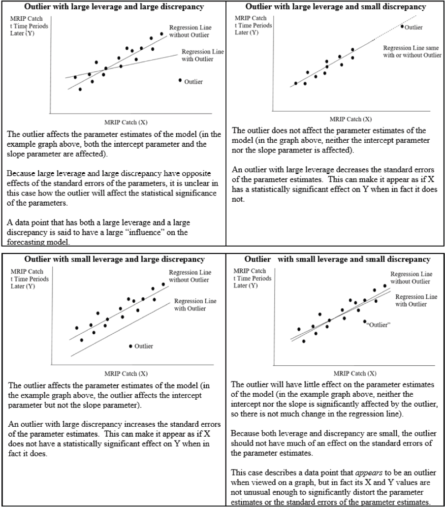
A plot of the leverage of each data point against the studentized residual of each data point can be used to assess potential outliers visually. Any data point that is in the upper-right quadrant of the graph (any data point with leverage h >2•(k/n) and studentized residual >2) has both a high leverage and a high studentized residual, and therefore could be considered an outlier. Such data points have the largest potential effects on the forecasting model—they can affect the parameter estimates (e.g., both the intercept and the slope in the graphs in Figure 4.2) as well as the standard errors and statistical significance of the parameter estimates.

Other, more advanced methods of outlier detection include Cook’s D value and DFITS values, which combine the leverage and discrepancy information in more sophisticated ways; Chauvenet’s criterion; Grubb’s test for outliers; Dixon’s Q test; Peirce’s criterion; Tukey’s fences; Mahalanobis distance; and the ASTM (American Society for Testing and Materials) E178 Standard Practice for Dealing with Outlying Observations. Sources that discuss issues related to identifying outliers in weighted survey responses, such as those produced by MRIP, include Hulliger (1995), Li and Valliant (2015) and section 5.2 of Heeringa et al. (2017).⁵⁷

Outliers may be of particular concern in design-based sampling programs, such as FES, that use Horvitz-Thompson variance estimates (Hulliger, 1995). In the presence of outliers, Horvitz-Thompson estimators remain unbiased, but the variance is increased. Sample observations of large magnitude with small inclusion probabilities have a particularly large influence on the Horvitz-Thompson estimator.

If an outlier is detected, there are five basic remedies:

• Leave the outlier in the dataset, but use a data transformation (such as logging X, Y, or both) to reduce the undesirable effects of the outlier.
• Leave the outlier in the dataset, but add a dummy variable to the dataset, where the dummy variable has the value 1 for the data observation with the outlier data point, and the value 0 otherwise. The purpose of the dummy variable is to represent the effects of variables outside the model that are affecting the outlier data point (i.e., causing it to be an outlier) but are not affecting the other data points.
• Replace the outlier in the dataset with the nearest, non-suspect data point (also known as “Winsorising”).
• Drop the outlier from the dataset (“trimming”).
• Leave the outlier in the dataset, but switch to a robust estimation modeling technique. Several approaches to robust estimation have been proposed, including R-estimators, L-estimators and M-estimators. M-estimators now appear to be preferred due to their generality and efficiency (Huber and Ronchetti, 2009; Hulliger, 1995).

If an outlier were to occur, fishery managers would first check to ensure that the outlier was not due to an error in the data or in data processing.⁵⁸ If the outlier was not due to an error, managers would need to decide whether (1) the outlier occurred because of chance alone, and so should not trigger a change in fishery management policies (e.g., a change in control rules); or (2) the outlier

___________________

⁵⁷ R software to implement some of the methods discussed by Li and Valliant can be found at: https://cran.r-project.org/web/packages/svydiags/index.html.

⁵⁸ The calibration methods used to correct for conversion of the CHTS to the FES, and the revised inclusion probabilities for the APAIS calibrations, could be sources of extreme values (outliers) in the calibrated MRIP estimates. Both calibration approaches were peer reviewed and found to be statistically sound. However, because the CHTS-FES calibrations resulted in varying increases in overall effort depending on year and region, and because the APAIS calibration also changed species-specific CPUE estimates, the chances of extreme values are increased. Hence, any extreme values in the calibrated estimates may be artifacts of the recalibration, despite their statistical rigor. Consideration of the joint effects of the methods used for CHTS-FES and APAIS calibrations on extreme value generation may be useful.

is an indication that either the fish population or the fishery is changing, and that as a result, the probability distribution of catch is shifting, and so the outlier should trigger a change in fishery management policies. Typically, fishery managers would use a prespecified level of statistical significance (say, 5 percent) to decide between (1) and (2). If the outlier exceeded the threshold value of catch based on the level of statistical significance, managers would decide that either the fish population or the fishery was changing, and that as a result, the probability distribution of catch was shifting, and so fishery management policies should be changed (or at least, further investigation would be warranted).

It is important to note that because of MRIP’s moderate sample size, it may not be possible to declare an individual estimate an outlier even when the underlying distribution has changed substantially. From the fishery manager’s perspective, it is necessary to consider the spatial, temporal, and species dependence in the catch estimates to detect change more effectively. For example, an isolated large decrease in the catch estimate for one species in one 2-month wave in one region may well be due to sampling error, whereas several moderate decreases in consecutive 2-month waves or multiple adjacent regions can be stronger evidence that the probability distribution of catch has changed and should trigger management action. Properly vetted multivariate spatiotemporal models for the fish population and fishery effort are essential to assess the strength of the evidence for change detection.

The type of change detection relevant to in-season management is online change detection. Popular methods include the CUSUM approach (Page, 1954; Verdier, 2020), the autoregressive models approach (Gombay, 2008; Tsay, 1988), and the Bayesian approach (Adams and MacKay, 2007; Barry and Hartigan, 1993). The Bayesian approach for online change detection is recommended for in-season management, and a simplified example is described in detail under the Bayesian model example of in-season management in Appendix D. Given a triggering outlier, the outlier value of catch (and its variance) could be used to update the probability distribution of fish catch using Bayesian updating methodology as described under that Bayesian model example. Other fisheries management policies (e.g., control rules) could then be updated based on the updated probability distribution of fish catch.

Order Statistics

In some cases, especially data-limited cases in which there are too few data points to develop a formal projection/forecasting model, fishing regulations have been based on ad hoc measures that attempt to find a balance between the “average” and the “variation” in the available MRIP catch estimates. An example of such a method is basing a catch forecast on “the third-largest of the five most recent MRIP catch estimates.” To find the threshold for identifying an outlier in such cases, one first needs to derive the probability distribution of such statistics, and here the concept of order statistics might be useful. Order statistics provide a method for determining the probabilities that the first-largest, second-largest, third-largest, etc., number in a set of numbers will take on particular values. For example, the method can be used to answer such questions as, “What is the probability that the third-largest annual MRIP estimate for a particular fish species out of the last five annual MRIP estimates for that species will be greater than 3,000 fish?” One possible definition of an outlier would be any such value with a chance of occurring that is less than the fishery managers’ preselected level of statistical significance (say, 5 percent). Appendix H presents a brief review of order statistics with a few simple fisheries management examples. Simulation studies should be used to compare alternative outlier detection methods before any particular method is adopted for a particular fishery.

Improved Partnerships and Collaborations

Effective and efficient coordination is of paramount importance given the range of federal, state, and regional organizations involved in surveys or analyses of recreational catch and effort. The MRIP Regional Implementation Teams and Interstate Fisheries Commission Fisheries Information Network (FIN) programs provide a valuable framework and structure for coordinating these interactions. For instance, Pacific RecFIN provides a good example of how a regional FIN system can facilitate successful coordination. Pacific RecFIN is led by the Pacific States Marine Fisheries Commission and involves coordinated sampling and data management across Washington, Oregon, and California. All three states implement locally tailored sampling programs to produce data on biological, social, and economic aspects of fisheries, and these data are ultimately contributed to a shared database. However, there are also recognized areas in which improvement is needed across all regions. For instance, the ACCSP Atlantic Coast Regional Implementation Plan stresses the importance of a continued emphasis on coordination as several state surveys that are not currently used in MRIP estimation could be used for this purpose later if MRIP certified. Another area for improvement involves the frequent need to calibrate recreational catch and effort estimates from various surveys. For instance, coordination is particularly critical in regions where survey methods may vary across states or specific fishery contexts, as well as when new survey programs are launched or modified. Finally, for all of these scenarios, effective and coordinated stakeholder engagement is critical for building and maintaining stakeholder trust and satisfaction in fisheries management. Chapter 5 builds upon these critical issues and looks at alternative surveys in the context of alternative management strategies.

CONCLUSIONS AND RECOMMENDATIONS

Conclusion: With strong support from fishery managers and stakeholders, MRIP and other recreational fisheries data collection programs have greatly improved the development and use of mobile apps and other electronic data collection and reporting platforms. While the use of these technologies can improve the efficiency of data collection, these technologies alone will not speed up the process if other systemic bottlenecks exist.

Conclusion: With additional resources, MRIP may be able to shorten by roughly 2 weeks the time between the end of its current bi-monthly reporting period and the release of preliminary estimates. This change would put additional stress on existing MRIP staff and systems, and for purposes of in-season management, the benefits of a modest advance in the release of preliminary estimates for bi-monthly waves would not be likely to justify the costs of accelerating the data processing and estimation phases of each bi-monthly cycle. It is possible that the raw MRIP data streams could be used to inform more timely catch estimates through such approaches as nowcasting or other in-season projection methods.

Conclusion: Given an approximate doubling of the resources that could be allocated to its survey programs, MRIP could transition to monthly catch estimates that would have levels of precision comparable to those of the current estimates for bi-monthly waves. For in-season management applications that rely on tracking MRIP estimates of cumulative catch against ACLs, the greatest advantage of moving to a 1-month cycle would lie in monitoring cumulative catch at the end of odd-numbered months. Other applications of MRIP data, including stock assessment and cross-year management of recreational fisheries (e.g., seasons, and catch and size limits), would also benefit from an MRIP transition to larger sample sizes required to maintain precision for monthly estimation of catch.

Conclusion: It is impractical to further improve the precision and timeliness of MRIP catch estimates to levels that could be achieved in the near-census catch reporting schemes used for the commercial sector, such as the VTR and SEFHIER programs. Any further improvements in MRIP precision and timeliness are therefore unlikely to be sufficient in and of themselves to achieve more effective in-season management of recreational fisheries. However, the committee identified a number of supplementary data sources and analytical approaches likely to improve the precision, timeliness, and adaptability of MRIP data for the purpose of improving catch forecasts for recreational fisheries subject to ACLs.

Conclusion: Further development of in-season management approaches utilizing novel statistical methods and additional data sources, such as state surveys, voluntary reporting, and analyses of social media posts, has the potential to improve incrementally the timeliness and precision of annual catch management. It is unlikely, however, that such approaches can replace MRIP as a source of spatially and temporally consistent catch information for monitoring and stock assessment of Council-managed stocks.

Conclusion: Because stock assessments rely on long time series of consistently collected data, and many federally managed stocks straddle state and survey boundaries, intercalibration of surveys is essential whenever a single survey is insufficient to support all assessment and management needs. Rigorous survey intercalibration requires temporal and spatial overlap between surveys. The need for intercalibration and the consequences of using different, uncalibrated surveys for various aspects of assessment and management are evident where different surveys provide very different estimates of the same unknown quantity (in the same units) and where the precision of surveys is perceived or known to differ.

Conclusion: Supplemental data in the form of state-specific recreational fishery surveys, species-specific surveys (e.g., Red Snapper), location-specific data, fishing tournament data, and voluntarily reported data (e.g., web portal– and smartphone-reported data) could be used in combination with MRIP estimates to improve in-season management. However, significant challenges would remain concerning the calibration and coordination of supplemental recreational catch and effort data with MRIP estimates. In addition to MRIP’s existing programs to calibrate state survey data collection and estimates with MRIP data and estimates, some of the methods discussed in this chapter could facilitate the integration of data from multiple sources.

Conclusion: A great variety of ancillary variables in readily accessible electronic format exist and potentially could be combined with MRIP catch estimates to improve the annual and in-season catch forecasts made in support of fishery management. When choosing which of the variety of ancillary variables available to use, one can consider that a variable will be more useful when the correlation (either positive or negative) between that variable and the catch of one or more recreational species is high. Ancillary variables that are also correlated with survey response propensity may be useful for reducing nonresponse bias. Furthermore, a particular ancillary variable will be more useful for the specific purpose of deciding when to close a fishery within a fishing season when that variable is available electronically with high frequency (i.e., daily or weekly).

Conclusion: If fishery managers are willing to accept some amount of bias in catch forecasts, it may be possible to use “Stein rule”–related statistical estimation methods to reduce the variance (PSEs) of catch forecasts and lower the overall MSE of the estimates. If justifiable restrictions (either equality or inequality restrictions) on model parameters can be identified, then incorporating such restrictions into the estimation methodology may reduce the MSE of the estimates.

Conclusion: Combining MRIP survey data with supplemental survey data using multiple-frame methods could decrease the variance (PSE) of catch estimates, depending on the relative sample sizes and catch variances of the combined surveys. Increasing the MRIP sample size decreases the value (in terms of variance reduction) of a supplemental survey. Increasing the sample size of a supplemental survey increases the value of that survey. An increase in the variance in catch within a supplemental survey increases the value of that survey. An increase in the variance in catch in the portion of the MRIP sample frame outside a supplemental survey sample frame decreases the benefit of that supplemental survey. As the size of a supplemental survey sample frame increases relative to the size of the MRIP sample frame, the benefit of that supplemental survey decreases.

Conclusion: Covariances between catch estimates from two different domains or between a catch estimate and an ancillary variable may be useful for reducing the variance and PSE of annual and in-season catch forecasts made by fishery managers who use MRIP output estimates in catch forecasting models. Conditional expectations of catch, conditional variances of catch, and the use of control variates may also be helpful for improving catch forecasts.

Conclusion: Spatiotemporal forecasting models, such as time-series cross-sectional models, SARIMA models, and SUR models, may be useful for developing catch forecasts for in-season management where data are sufficient. It may be necessary to combine MRIP catch estimates with data from supplementary surveys and on ancillary variables to achieve needed forecast accuracy and precision. These models can be used to address the statistical issues of heteroskedasticity, temporal autocorrelation, and contemporaneous correlation to improve the accuracy and precision of catch forecasts. The time-series forecasting models of Farmer and Froeschke (2015) and Farmer et al. (2020) are good examples of the potential use of time-series SARIMA methods for building applied, managerially relevant, in-season catch forecasting models. These models integrate MRIP and supplementary survey data as well as ancillary variables (stock status, weather, economic conditions, etc.) to forecast in-season catch, determine appropriate season length, and control the probability of exceeding an ACL.

Conclusion: The SUR method may be useful for reducing the variance and PSEs of catch forecasts when the errors across domains (e.g., across fish species) are contemporaneously correlated; that is, when the errors in different domains move together. When errors are contemporaneously correlated, it may be possible to improve forecasts by estimating systems of equations together, for example, by estimating together the forecasting models for multiple fish species. The SUR method can accommodate heteroskedasticity and temporal autocorrelation.

Conclusion: Bayesian modeling methodology may serve as a good overarching framework for regional federal and state fishery managers to use in integrating and updating MRIP catch estimates, supplemental survey data, and ancillary variables for the purpose of producing annual catch forecasts and in-season catch forecasts. Furthermore, many, if not all, of the other methodological approaches described in this report can be integrated within a Bayesian framework. The Bayesian methodology provides a consistent approach to handling uncertainty and risk and supporting probabilistic decision making, such as decisions about when to close seasonal fisheries to maintain the probability of exceeding ACLs below fishery managers’ tolerance level. The existence of widely available software for implementing Bayesian models facilitates their use in fishery management.

Conclusion: For some rare-event species, the distribution of catch in catch forecasts may be better modeled using a probability distribution other than the normal distribution. Examples of such distributions include the Poisson, negative binomial, zero-inflated Poisson, and zero-inflated negative binomial. Statistical methods exist for determining when the use of one distribution would be better (lower error in catch forecasts) than another.

Conclusion: The method of inverse sampling may be useful for estimating the population or catch of some rare-event species, especially in situations in which the catch of the rare-event species is very low and sporadic, with zero catches in some locations and time periods.

Conclusion: For some rare-event species, especially newly discovered species or those with very little catch data, the combined use of uninformative priors, an assumption of catch proportional to abundance, and Bayesian updating may be useful for forecasting the catch of that species. When fishery-independent estimates of the total fish population (all species together) exist, the method may also be useful for estimating the population of the rare-event species as well. This method is a special case of the general Bayesian modeling framework discussed elsewhere in this report.

Conclusion: Traditional statistical methods can be used to define and identify outlier catch estimates in cases in which sufficient data are available. Order statistics may be useful for defining and identifying outliers in data-limited situations in which it may not be possible to apply the traditional methods. Change detection methods in time-series data analysis, including Bayesian approaches, can be used to help answer the question of when an outlier should trigger management change.

REFERENCES

Cruze, N. B. 2016. A Bayesian hierarchical model for combining several crop yield indications. JSM Proceedings, Survey Research Methods Section, pp. 2045–2053. Alexandria, VA: American Statistical Association.

Cruze, N. B., and H. K. Benecha. 2017. A model-based approach to crop yield forecasting. JSM Proceedings, Survey Research Methods Section, pp. 2724–2733. Alexandria, VA: American Statistical Association.

Cruze, N. B., A. L. Erciulesscu, B. Nandram, W. J. Barboza, and L. J. Young. 2016. Developments in model-based estimation of county-level agricultural estimates. Paper presented at the Fifth International Conference on Establishment Surveys, Geneva, Switzerland, June 20–23. http://ww2.amstat.org/meetings/ices/2016/proceedings/131_ices15Final00229.pdf.

Cruze, N. B., A. L. Erciulescu, B. Nandram, W. J. Barboza, and L. J. Young. 2019. Producing official county-level agricultural estimates in the United States: Needs and challenges. Statistical Science 34(2):301–316.

DeGroot, M. H. 1970. Optimal Statistical Decisions. New York: McGraw-Hill.

DeGroot, M. H. 1980. Improving predictive distributions. In Bayesian Statistics, J. M. Bernardo, M. H. DeGroot, D. V. Lindley, and A. F. M. Smith, eds. Valencia, Spain: University Press.

Doll, J. C. and S. J. Jacquemin. 2018. Introduction to Bayesian modeling and inference for fisheries scientists. Fisheries 43(3):152–161.

Dumas, C. F. 2021. Economic Impact Analysis of North Carolina’s Commercial Fisheries—Commercial Harvesters Survey. DEQ Task Order No. 8007. Morehead City, NC: North Carolina Department of Environmental Quality, Division of Marine Fisheries. https://ncseagrant.ncsu.edu/wp-content/uploads/2021/02/NC-Commercial-Fishing-Survey.pdf.

Dundas, S. J., and R. H. von Haefen. 2020. The effects of weather on recreational fishing demand and adaptation: Implications for a changing climate. Journal of the Association of Environmental and Resource Economists 7(2):209–242.

Durbin, J. 1970. Testing for serial correlation in least-squares regression when some of the regressors are lagged dependent variables. Econometrica 38:410–421.

Efron, B., and C. Morris. 1973. Stein’s estimation rule and its competitors—An empirical Bayes approach. Journal of the American Statistical Association 68:117–130.

Efron, B., and C. Morris. 1975. Data analysis using Stein’s estimator and its generalizations. Journal of the American Statistical Association 70:311–319.

Engle, R. F. 1982. Autoregressive conditional heteroscedasticity with estimates of the variance of United Kingdom inflations. Econometrica 50:987–1008.

Englin, J., and J. S. Shonkwiler. 1995. Estimating social welfare using count data models: An application to long-run recreation demand under conditions of endogenous stratification and truncation. Review of Economics and Statistics 77:104–112.

English, E., R. H. von Haefen, J. Herriges, C. Leggett, F. Lupi, K. McConnell, M. Welsh, A. Domanski, and N. Meade. 2018. Estimating the value of lost recreation days from the Deepwater Horizon oil spill. Journal of Environmental Economics and Management 91:26–45.

Erciulescu, A. L., N. B. Cruze, and B. Nandram. 2018. Benchmarking a triplet of official estimates. Environmental and Ecological Statistics 25:523–547. https://doi.org/10.1007/s10651-018-0416-4.

Erciulescu, A. L., N. B. Cruze, and B. Nandram. 2019. Model-based county-level crop estimates incorporating auxiliary sources of information. Journal of the Royal Statistical Society, Series A 182(1):283–303. https://doi.org/10.1111/rssa.12390.

Fackler, P. L. 2014. Structural and observational uncertainty in environmental and natural resource management. International Review of Environmental and Resource Economics 7(2):109–139.

Farmer, N. A., and J. T. Froeschke. 2015. Forecasting for recreational fisheries management: What’s the catch? North American Journal of Fisheries Management 35:720–735.

Farmer, N. A., J. T. Froeschke, and D. L. Records. 2020. Forecasting for recreational fisheries management: A derby fishery case study with Gulf of Mexico Red Snapper. ICES Journal of Marine Science 77(6):2265–2284. https://doi.org/10.1093/icesjms/fsz238.

Fay, R. E., III, and R. A. Herriot. 1979. Estimates of income for small places: An application of James-Stein procedures to census data. Journal of the American Statistical Association 74:269–277.

Flickr Services. 2021. The App Garden: API Documentation. https://www.flickr.com/services/api.

Foster, J., and D. V. Voorhees. 2015. Methods for Improving Precision of Catch Statistics for Deepwater Species: Custom Estimation Methods. NOAA Fisheries, Office of Science and Technology—Fisheries Statistics Division. Presentation to South Atlantic Fishery Management Council, Scientific and Statistical Committee Meeting, October 21, 2015.

Fraidenburg, M. E., and G. G. Bargmann. 1982. Estimating boat-based fishing effort in a marine recreational fishery. North American Journal of Fisheries Management 2:351–358.

Fuller, W. A., and L. F. Burmeister. 1972. Estimators for samples selected from two overlapping frames. Proceedings of the Social Statistics Section of the American Statistical Association, pp. 245–249.

Fuller, W. A., and J. N. K. Rao. 2001. A regression composite estimator with application to the Canadian Labour Force Survey. Survey Methodology 27(1):45–52.

GAFGI (Gulf Angler Focus Group Initiative). 2017. Examination of Possible Private Recreational Management Options for Gulf of Mexico Red Snapper. Alexandria, VA: American Sportfishing Association.

Gallaway, B. J., J. G. Cole, L. R. Martin, J. M. Nance, and M. Longnecker. 2003. An evaluation of an electronic logbook as a more accurate method of estimating spatial patterns of trawling effort and bycatch in the Gulf of Mexico shrimp fishery. North American Journal of Fisheries Management. 23:787–809.

Gentner, B., and S. Sutton. 2008. Substitution in recreational fishing. Global Challenges in Recreational Fisheries, pp. 150–169.

Geronimo, R. C., E. C. Franklin, R. E. Brainard, C. D. Elvidge, M. D. Santos, R. Venegas, and C. Mora. 2018. Mapping fishing activities and suitable fishing grounds using nighttime satellite images and maximum entropy modelling. Remote Sensing 10(10):1604.

Gillig, D., T. Ozuna, Jr., and W. L. Griffin. 2000. The value of the Gulf of Mexico recreational Red Snapper fishery. Marine Resource Economics 15:127–139.

Glaab, J. 2017. Extracting Parking Areas from Remote Sensing Imagery and Spatiotemporal Traffic Data. Master’s Thesis, University of Rhode Island. https://doi.org/10.23860/thesis-glaab-julian-2017.

GMFMC (Gulf of Mexico Fishery Management Council). 2019. Modification to the Recreational For-Hire Red Snapper Annual Catch Target Buffer: Framework Action to the Fishery Management Plan for the Reef Fish Resources of the Gulf of Mexico Including Draft Environmental Assessment, Regulatory Impact Review, and Regulatory Flexibility Act Analysis. Tampa, FL: Gulf of Mexico Fishery Management Council.

Gombay, E. 2008. Change detection in autoregressive time series. Journal of Multivariate Analysis 99(3):451–464.

Gorelick, N., M. Hancher, M. Dixon, S. Ilyushchenko, D. Thau, and R. Moore. 2017. Google Earth Engine: Planetary-scale geospatial analysis for everyone. Remote Sensing of Environment 202:18–27.

Groves, R. 1989. Survey Errors and Survey Costs. New York: Wiley.

GulfFIN (Gulf Fisheries Information Network). 2016. GulfFIN MRIP Implementation Plan (2016–2018). https://www.fisheries.noaa.gov/resource/document/mrip-regional-implementation-plan-gulf-coast-2016-2018.

Haab, T. C., and K. E. McConnell. 1996. Count data models and the problem of zeros in recreation demand analysis. American Journal of Agricultural Economics 78:89–102.

Haddad, K. 2017. Gulf Angler Focus Group Initiative: Process Overview and Identified Management Options. Alexandria, VA: American Sportfishing Association.

Haldane, J. B. S. 1945. On a method of estimating frequencies. Biometrika 33(3):222–225.

Hann, C. H., L. L. Stelle, A. Szabo, and L. G. Torres. 2018. Obstacles and opportunities of using a mobile app for marine mammal research. ISPRS International Journal of Geo-Information 7(5):169.

Hansen, M. H., W. N. Hurwitz, and W. G. Madow. 1953. Sample survey methods and theory, volume 1. New York: Wiley.

Hanson, P. J., D. S. Vaughan, and S. Narayan. 2006. Forecasting annual harvests of Atlantic and Gulf menhaden. North American Journal of Fisheries Management 26:753–764.

Hartley, H. O. 1962. Multiple frame surveys. Proceedings of the Social Science Section of the American Statistical Association, pp. 203–206.

Hartley, H. O. 1974. Multiple frame methodology and selected applications. Sankhya, Series C 36:99–118.

Hauser, C. E., and H. P. Possingham. 2008. Experimental or precautionary? Adaptive management over a range of time horizons. Journal of Applied Ecology 45(1):72–81.

Hawkins, D. M. 1980. Identification of Outliers, Volume 11. London, UK: Chapman and Hall.

Heeringa, S. G., B. T. West, and P. A. Berglund. 2017. Applied Survey Data Analysis, 2nd Edition. Boca Raton, FL: Chapman and Hall.

Hellerstein, D. M., and R. Mendelsohn. 1993. A theoretical foundation for count data models. American Journal of Agricultural Economics 75:604–611.

Hendry, D. F., and J. F. Richard. 1983. The econometric analysis of economic time series. International Statistical Review 51:111–163.

Hey, J. D. 1985. Data in Doubt—An Introduction to Bayesian Statistical Inference for Economists. Oxford, UK: Basil Blackwell.

Hinz, H., L. G. Murray, G. I. Lambert, J. G. Hiddink, and M. J. Kaiser. 2013. Confidentiality over fishing effort data threatens science and management progress. Fish and Fisheries 14:110–117.

Hsiang, S., R. Kopp, A. Jina, J. Rising, M. Delgado, S. Mohan, D. J. Rasmussen, R. Muir-Wood, P. Wilson, M. Oppenheimer, K. Larsen, and T. Houser. 2017. Estimating economic damage from climate change in the United States. Science 356(6345):1362–1369.

Huber, P. J., and E. M. Ronchetti. 2009. Robust Statistics, 2nd Edition. New York: Wiley, p. 370.

Hulliger, B. 1995. Outlier robust Horvitz-Thompson estimators. Survey Methodology 21(1):79–87.

Ives, A. R., K. C. Abbott, and N. L. Ziebarth. 2010. Analysis of ecological time series with ARMA(p,q) models. Ecology 91:858–871.

James, W., and C. Stein. 1961. Estimation with quadratic loss. Proceedings of the Fourth Berkeley Symposium on Mathematical Statistics and Probability, pp. 361–379. Berkeley, CA: University of California Press.

Jiorle, R. P., R. N. M. Ahrens and M. S. Allen. 2016. Assessing the utility of a smartphone app for recreational fishery catch data. Fisheries 41(12):758–766.

Judge, G. G., and M. E. Bock. 1978. The Statistical Implications of Pre-Test and Stein Rule Estimators in Econometrics. New York: North-Holland.

Judge, G. G., and M. E. Bock. 1983. Biased estimation. In Handbook of Econometrics, pp. 599–650. Amsterdam, The Netherlands: North Holland.

Judge, G. G., W. E. Griffiths, R. C. Hill, H. Lutkepohl, and T-C. Lee. 1985. The Theory and Practice of Econometrics, 2nd Edition. New York: Wiley.

Kalton, G., and D. W. Anderson. 1986. Sampling rare populations. Journal of the Royal Statistical Society, Series A 149:65–82.

Kim, J. K., and J. N. Rao. 2012. Combining data from two independent surveys: A model-assisted approach. Biometrika 99(1):85–100.

Kim, J. K., and S. M. Tam. 2021. Data integration by combining big data and survey sample data for finite population inference. International Statistical Review 89(2):382–401. https//doi.org/10.1111/insr.12434.

Kim, J. K., Z. Wang, Z. Zhu, and N. B. Cruze. 2018. Combining survey and non-survey data for improved sub-area prediction using a multi-level model. Journal of Agricultural, Biological and Environmental Statistics 23(2):175–189.

King, R., and R. McCrea. 2019. Capture–recapture methods and models: Estimating population size. In Handbook of Statistics, Volume 40: Integrated Population Biology and Modeling, Part B, A. S. R. S. Rao and C. R. Rao, eds., p. 635. https://doi.org/10.1016/bs.host.2018.09.006.

Kirtman, B. P., D. Min, J. M. Infanti, J. L. Kinter III, D. A. Paolino, Q. Zhang, H. van den Dool, S. Saha, M. Pena Mendez, E. Becker, P. Peng, P. Tripp, J. Huang, D. G. DeWitt, M. K. Tippett, A. G. Barnston, S. Li, A. Rosati, S. D. Schubert, M. Rienecker, M. Suarez, Z. E. Li, J. Marshak, Y. Lim, J. Tribbia, K. Pegion, W. J. Merryfield, B. Denis, and E. F. Wood. 2014. The North American multimodel ensemble: Phase-1 seasonal-to-interannual prediction; Phase-2 toward developing intraseasonal prediction. Bulletin of the American Meteorological Society 95(4):585–601. https://doi.org/10.1175/BAMS-D-12-00050.1.

Kroodsma, D. A., J. Mayorga, T. Hochberg, N. A. Miller, K. Boerder, F. Ferretti, A. Wilson, B. Bergman, T. D. White, B. A. Block, P. Woods, B. Sullivan, C. Costello, and B. Worm. 2018. Tracking the global footprint of fisheries. Science 359(6378):904–908.

Lambrides, A., T. Wolfe, K. Le, and P. Jahnig. 2018. Satellite Image Finder Parking Lot & Spots—Final Report. Blacksburg, VA: Department of Computer Science, Virginia Tech. https://vtechworks.lib.vt.edu/bitstream/handle/10919/83200/SatelliteImageFinderReport.pdf?sequence=19&isAllowed=y.

LaRiviere, J., D. Kling, J. N. Sanchirico, C. Sims, and M. Springborn. 2018. The treatment of uncertainty and learning in the economics of natural resource and environmental management. Review of Environmental Economics and Policy 12(1):92–112.

Lazar, R., G. Meeden, and D. Nelson. 2008. A noninformative Bayesian approach to finite population sampling using auxiliary variables. Survey Methodology 34:51–64.

Lee, M., S. Steinback, and K. Wallmo. 2017. Applying a bioeconomic model to recreational fisheries management: Groundfish in the Northeast United States. Marine Resource Economics 32:191–216.

Li, J., and R. Valliant. 2015. Linear regression diagnostics in cluster samples. Journal of Official Statistics 31(1):61–75.

Liu, B., S. L. Stokes, T. Topping, and G. Stunz. 2017. Estimation of a total from a population of unknown size and application to estimating recreational Red Snapper catch in Texas. Journal of Survey Statistics and Methodology 5:350–371.

Lohr, S. L., and T. E. Raghunathan. 2017. Combining survey data with other data sources. Statistical Science 32:293–312.

Lohr, S. L., and J. N. K. Rao. 2000. Inference in dual frame surveys. Journal of the American Statistical Association 95:271–280.

Lohr, S. L., and J. N. K. Rao. 2006. Estimation in multiple-frame surveys. Journal of the American Statistical Association 101(475):1019–1030.

Long, J. S. 1997. Regression Models for Categorical and Limited Dependent Variables. Thousand Oaks, CA: Sage Publications.

Madans, J. H., T. M. Ezzati-Rice, M. Cynamon, and S. J. Blumberg. 2001. Targeting approaches to state-level estimates. In Proceedings of the Seventh Conference on Health Survey Research Methods, M. L. Cynamon and R. A. Kulka, eds., pp. 239–245. Hyattsville, MD: U.S. Department of Health and Human Services.

Makridakis, S., S. C. Wheelwright, and R. J. Hyndman. 2008. Forecasting Methods and Applications. New York: Wiley.

Mancini, F., G. M. Coghill, and D. Lusseau. 2018. Using social media to quantify spatial and temporal dynamics of nature-based recreational activities. PLoS One 13(7):e0200565. https://doi.org/10.1371/journal.pone.0200565.

Massetti, E., and R. Mendelsohn. 2018. Measuring climate adaptation: Methods and evidence. Review of Environmental Economics and Policy 12(2):324–341.

Mercer, L., J. Wakefield, A. Pantazis, A. Lutambi, H. Masanja, and S. Clark. 2015. Small area estimation of child mortality in the absence of vital registration. Annals of Applied Statistics 9(4):1889–1905.

Merrill, N. H., S. F. Atkinson, K. K. Mulvaney, M. J. Mazzotta, and J. Bousquin. 2020. Using data derived from cellular phone locations to estimate visitation to natural areas: An application to water recreation in New England, USA. PLoS One 15(4):e0231863. https://doi.org/10.1371/journal.pone.0231863.

Midway, S. R., J., Adriance, P. Banks, S. Haukebo, and R. Caffey. 2020. Electronic self-reporting: Angler attitudes and behaviors in the recreational Red Snapper fishery. North American Journal of Fisheries Management 40:1119–1132. doi: 10.1002/nafm.10472.

Molina, I., and Y. Marhuenda. 2015. SAE: An R package for small area estimation. R Journal. http://cran.r-project.org/web/packages/sae/sae.pdf.

Molina, I., and Y. Marhuenda. 2020. Small Area Estimation: Package “sae,” Version 1.3. http://cran.r-project.org/web/packages/sae/sae.pdf.

Morley, J. W., R. L. Selden, R. J. Latour, T. L. Frolicher, R. J. Seagraves, and M. L. Pinsky. 2018. Projecting shifts in thermal habitat for 686 species on the North American continental shelf. PLoS One 13(5):e0196127.

Mukhopadhyay, P. K., and A. McDowell. 2011. Small area estimation for survey data analysis using SAS® software. Proceedings, SAS Global Forum 2011, Paper 336-2011. http://support.sas.com/resources/papers/proceedings11/336-2011.pdf.

Nandram, B., E. Berg, and W. Barboza. 2014. A hierarchical Bayesian model for forecasting state-level corn yield. Environmental and Ecological Statistics 21:507–530.

Nandram, B., A. L. Erciulescu, and N. Cruze. 2019. Bayesian benchmarking of the Fay-Herriot model using random deletion. Survey Methodology 45(2):365–390. https://www150.statcan.gc.ca/n1/pub/12-001-x/2019002/article/00004-eng.htm.

NASEM (National Academies of Sciences, Engineering, and Medicine). 2017a. Review of the Marine Recreational Information Program. Washington, DC: The National Academies Press. https://doi.org//10.17226/24640.

NASEM. 2017b. Improving Crop Estimates by Integrating Multiple Data Sources. Washington, DC: The National Academies Press. https://doi.org/10.17226/24892.

NCDMF (North Carolina Department of Environmental Quality, Division of Marine Fisheries). 2021. Trip Ticket Program. Morehead City, NC. http://portal.ncdenr.org/web/mf/46.

NDBC (National Data Buoy Center). 2015. NDBC Web Data Guide. Stennis Space Center, MS: National Oceanic and Atmospheric Administration. https://www.ndbc.noaa.gov/docs/ndbc_web_data_guide.pdf.

NMFS-SERO (National Marine Fisheries Service-Southeast Regional Office). 2013. Updated 2013 Gulf of Mexico Red Snapper Recreational Season Length Estimates. SERO-LAPP-2012-02 (Addendum). May 21, updated June 4. St. Petersburg, FL: NOAA.

NMFS-SERO. 2014. 2014 Gulf of Mexico Red Snapper Recreational Season Length Estimates (Revised and Updated). SERO-LAPP-2014-04. April 21, 2014. St. Petersburg, FL: NOAA. http://sero.nmfs.noaa.gov/sustainable_fisheries/lapp_dm/documents/pdfs/2014/red_Snapper_2014_season_length.pdf.

NMFS-SERO. 2015. 2015 Gulf of Mexico Red Snapper Recreational Season Length Estimates. SERO-LAPP-2015-04. April 20. St. Petersburg, FL: NOAA. http://sero.nmfs.noaa.gov/sustainable_fisheries/lapp_dm/documents/pdfs/2015/rs_2015_rec_quota_projection.pdf.

NMFS-SERO. 2016. 2016 Gulf of Mexico Red Snapper Recreational Season Length Estimates. SERO-LAPP-2014-04. May 2. St. Petersburg, FL: NOAA. http://sero.nmfs.noaa.gov/sustainable_fisheries/lapp_dm/documents/pdfs/2016/sero-lapp-2016-04_gom_red_Snapper_rec_season_2016_20160502_sero_final.pdf.

NOAA Fisheries (National Marine Fisheries Service of the National Oceanic and Atmospheric Administration). 2019a. Marine Recreational Information Program, Research and Evaluation Team Review of the iAngler and iSnapper Reporting Programs. https://media.fisheries.noaa.gov/dam-migration/mrip_ret_review_of_iangler_and_iSnapper_reporting_programs_05-10-2019.pdf.

NOAA Fisheries. 2019b. NOAA Fisheries Explores Electronic Reporting as Supplemental Source of Recreational Fishing Data. News, July 26. https://www.fisheries.noaa.gov/feature-story/noaa-fisheries-explores-electronic-reporting-supplemental-source-recreational-fishing.

NOAA NHC (National Oceanic and Atmospheric Administration National Hurricane Center). 2021. New Experimental Weather Forecast Elements Added for “Blue Water” Mariners South-Atlantic. https://www.nhc.noaa.gov/news/Whats_New_Marine_Composite_Page.pdf.

NRC (National Research Council). 2000. Small-Area Income and Poverty Estimates: Priorities for 2000 and Beyond. Washington, DC: National Academy Press. https://doi.org/10.17226/9957.

NRC. 2006. Review of Recreational Fisheries Survey Methods. Washington, DC: The National Academies Press. https://doi.org/10.17226/11616.

Obradovich, N., and J. H. Fowler. 2017. Climate change may alter human physical activity patterns. Nature Human Behavior 1:0097.

ODFW (Oregon Department of Fish and Wildlife). 2012. Oregon Recreational Groundfish Model for 2013/2014. Salem, OR: ODFW.

ODFW. 2021. Environmental Defense Fund (EDF) Launches SmartPass Initiative to Help Manage Ocean Fishing: Smart Cameras and AI Can Help Ensure Sustainable Fisheries, Ease Burden of Data Collection. News Release. February 18. Salem, OR. https://www.dfw.state.or.us/news/2021/02_feb/021821.asp.

Oh, C.-O., S. G. Sutton, and M. G. Sorice. 2013. Assessing the role of recreation specialization in fishing site substitution. Leisure Sciences 35(3):256–272.

Opsomer, J. D., C. Botts, and J. Y. Kim. 2003. Small area estimation in a watershed erosion assessment survey. Journal of Agricultural, Biological, and Environmental Statistics 8:139–152.

Ozuna, T., Jr., and I. A. Gomez. 1994. Estimating a system of recreation demand functions using a seemingly unrelated Poisson regression approach. Review of Economics and Statistics 76:356–360.

Ozuna, T., Jr., and I. A. Gomez. 1995. Specification and testing of count data recreation demand functions. Empirical Economics 20:543–550.

Page, E. S. 1954. Continuous inspection schemes. Biometrika 41(1/2):100–115.

Papacostas, K. J., and J. Foster. 2018. Survey Design and Statistical Methods for Estimation of Recreational Fisheries Catch and Effort, 2018—Version 1. National Marine Fisheries Service’s Marine Recreational Information Program. Updated March 2021. https://media.fisheries.noaa.gov/2021-09/MRIP-Survey-Design-and-Statistical-Methods-2021-09-15.pdf.

Papenfuss, J. T., N. Phelps, D. Fulton, and P. A. Venturelli. 2015. Smartphones reveal angler behavior: A case study of a popular mobile fishing application in Alberta, Canada. Fisheries 40:318–327.

Park, S., J. K. Kim, and D. Stukel. 2017. A measurement error model approach to survey data integration: Combining information from two surveys. METRON 75(3):345–357.

Pesando, J. E. 1972. Seasonal variability in distributed lag models. Journal of the American Statistical Association 67:311–312.

Pfeffermann, D., and C. Barnard. 1991. Some new estimators for small area means with application to the assessment of farmland values. Journal of Business and Economic Statistics 9:31–42.

Pinsky, M. L., B. Worm, M. J. Fogarty, J. L. Sarmiento, and S. A. Levin. 2013. Marine taxa track local climate velocities. Science 341(6151):1239–1242.

Powers, S. P., and K. Anson. 2016. Estimating recreational effort in the Gulf of Mexico Red Snapper fishery using boat ramp cameras: Reduction in federal season length does not proportionally reduce catch. North American Journal of Fisheries Management 36(5):1156–1166. https://doi.org/10.1080/02755947.2016.1198284.

Powers, S. P. and K. Anson. 2019. Compression and relaxation of fishing effort in response to changes in length of fishing season for Red Snapper (Lutjanus campechanus) in the northern Gulf of Mexico. Fisheries Bulletin 117:1–7. https://doi.org/10.7755/FB.117.1.1.

Powers, S. P., F. J. Fodrie, S. B. Scyphers, J. M. Drymon, R. L. Shipp, and G. W. Stunz. 2013. Gulf-wide decreases in the size of large coastal sharks documented by generations of fishermen. Marine and Coastal Fisheries: Dynamics, Management, and Ecosystem Science 5(5):92–102. https://doi.org/10.1080/19425120.2013.786001.

Punt, A., and R. Hilborn. 1997. Fisheries stock assessment and decision analysis: The Bayesian approach. Reviews in Fish Biology and Fisheries 7(1):35–63.

Rao, J. N. K. 2003. Small Area Estimation, 1st Edition. Hoboken, NJ: John Wiley & Sons.

Rao, J. N. K. 2021. On making valid inferences by combining data from surveys and other sources. Sankhya B 83:242–272. https://doi.org/10.1007/s13571-020-00227-w.

Rao, J. N. K., and I. Molina. 2015. Small Area Estimation, 2nd Edition. Hoboken, NJ: John Wiley & Sons.

Rao, J. N. K., and M. Yu. 1992. Small area estimation combining time series and cross-sectional data. Proceedings of the Survey Research Methods Section of the American Statistical Association, pp. 1–9. http://www.asasrms.org/Proceedings/papers/1992_001.pdf.

Rao, J. N. K., and M. Yu. 1994. Small area estimation by combining time-series and cross sectional data. Canadian Journal of Statistics 22:511–528.

Rehage, J. S., R. O. Santos, E. K. N. Kroloff, J. T. Heinen, Q. Lai, B. D. Black, R. E. Boucek, and A. J. Adams. 2019. How has the quality of bonefishing changed over the past 40 years? Using local ecological knowledge to quantitatively inform population declines in the South Florida flats fishery. Environmental Biology of Fishes 102(2):285–298.

Rout, T. M., C. E. Hauser, and H. P. Possingham. 2009. Optimal adaptive management for the translocation of a threatened species. Ecological Applications 19(2):515–526.

Ruiz, J., I. Caballero, and G. Navarro. 2020. Sensing the same fishing fleet with AIS and VIIRS: A seven-year assessment of squid jiggers in FAO Major Fishing Area 41. Remote Sensing 12(1):32.

Salz, R., D. Van Vorhees, G. Colton, and J. Rosetti. 2011. Addressing the Fishery Management Need for More Timely Recreational Data. MRIP Final Project Report. Marine Recreational Information Program. NOAA Fisheries. https://media.fisheries.noaa.gov/dam-migration/mrip-addressing-the-fishery-management-need-for-more-timely-recreational-data-2011.pdf.

Sauls, B., and D. Lazarre. 2019. Recreational Effort, Catch and Biological Sampling in Florida During the 2019 South Atlantic Red Snapper Season. Final Report F4451-19-F. St. Petersburg, FL: Florida Fish and Wildlife Conservation Commission.

Sauls, B., R. P. Cody, and A. J. Strelcheck. 2017. Survey methods for estimating Red Snapper landings in a high-effort recreational fishery managed with a small annual catch limit. North American Journal of Fisheries Management 3(2):302–313. https://doi.org/10.1080/02755947.2016.1264512.

Singh, A. C. 1994. Sampling design based estimating functions for finite population totals. Invited paper, Abstracts of the Annual Meeting of the Statistical Society of Canada, Banff, Alberta, May 811, p. 48.

Skinner, C. J. 1991. On the efficiency of raking ratio estimation for multiple frame surveys. Journal of the American Statistical Association 86:779–784.

Skinner, C. J., and J. N. K. Rao. 1996. Estimation in dual frame surveys with complex designs. Journal of the American Statistical Association 91:349–356.

Specht, C., P. S. Dabrowski, J. Pawelski, M. Specht, and T. Szot. 2019. Comparative analysis of positioning accuracy of GNSS receivers of Samsung Galaxy smartphones in marine dynamic measurements. Advances in Space Research 63(9):3018–3028.

Springborn, M. R. 2014. Risk aversion and adaptive management: Insights from a multi-armed bandit model of invasive species risk. Journal of Environmental Economics and Management 68(2):226–242.

Springborn, M., and J. N. Sanchirico. 2013. A density projection approach for non-trivial information dynamics: Adaptive management of stochastic natural resources. Journal of Environmental Economics and Management 66(3):609–624.

Staton, B. A., and M. J. Catalano. 2019. Bayesian information updating procedures for Pacific Salmon run size indicators: Evaluation in the presence and absence of auxiliary migration timing information. Canadian Journal of Fisheries and Aquatic Sciences 76(10):1719–1727.

Staton, B., and H. Hershey. 2020. Introductory Bayesian Inference with JAGS in Fisheries Science. Continuing Education Workshop, American Fisheries Society annual meeting, September 28, 2020.

Stein, C. 1955. Inadmissibility of the usual estimator for the mean of a multivariate normal distribution. Proceedings of the Third Berkeley Symposium on Mathematical Statistics and Probability, pp. 197–206. Berkeley, CA: University of California Press.

Stergiou, K., and E. Christou. 1996. Modelling and forecasting annual fisheries catches: Comparison of regression, univariate and multivariate time series methods. Fisheries Research 25:105–138.

Stokes, S. L., B. M. Williams, R. P. A. McShane, and Z. Zalsha. 2021. The impact of nonsampling errors on estimators of catch from electronic reporting systems. Journal of Survey Statistics and Methodology 9(1):159–184. https://doi.org/10.1093/jssam/smz042.

Sutton, S. G., and C. O. Oh. 2015. How do recreationists make activity substitution decisions? A case of recreational fishing. Leisure Sciences 37(4):332–353.

Tol, R. S. 2014. Correction and update: The economic effects of climate change. Journal of Economic Perspectives 28(2):221–225.

Tourangeau, R., E. English, K. E. McConnell, D. Chapman, I. F. Cervantes, E. Horsch, N. Meade, A. Domanski, and M. Welsh. 2017. The Gulf Recreation Study: Assessing lost recreational trips from the 2010 Gulf oil spill. Journal of Survey Statistics and Methodology 5(3):281–309.

Tsay, R. S. 1988. Outliers, level shifts, and variance changes in time series. Journal of Forecasting 7(1):1–20.

USBR (U.S. Bureau of Reclamation). 2013. Downscaled CMIP3 and CMIP5 Climate and Hydrology Projections. Denver, CO: Technical Services Center, Bureau of Reclamation, U.S. Department of the Interior. https://gdo-dcp.ucllnl.org/downscaled_cmip_projections.

USNWS (U.S. National Weather Service). 2019. Hurricane Dorian—September 6, 2019. Newport/Morehead City, NC: Weather Forecast Office, National Weather Service, NOAA. https://www.weather.gov/mhx/Dorian2019.

Verdier, G. 2020. An empirical likelihood-based CUSUM for on-line model change detection. Communications in Statistics—Theory and Methods 49(8):1818–1839.

Wang, J. C., S. H. Holan, B. Nandram, W. Barboza, C. Toto, and E. Anderson. 2012. A Bayesian approach to estimating agricultural yield based on multiple repeated surveys. Journal of Agricultural, Biological and Environmental Statistics 17:84–106.

Wang, X., E. Berg, Z. Zhu, D. Sun, and G. Demuth. 2018. Small area estimation of proportions with constraint for National Resources Inventory Survey. Journal of Agricultural, Biological and Environmental Statistics 23:509–528.

Whitehead, J. C., B. Poulter, C. F. Dumas, and O. Bin. 2009. Measuring the economic effects of sea level rise on shore fishing. Mitigation and Adaptation Strategies for Global Change 14(8):777–792.

Wieand, K. 2008. A Bayesian methodology for estimating the impacts of improved coastal ocean information on the marine recreational fishing industry. Coastal Management 36(2):208–223.

Young, E. G., M. C. Melnychuk, L. E. Anderson, and R. Hilborn. 2020. The importance of fishing opportunity to angler utility analysis in marine recreational fisheries. ICES Journal of Marine Science. 77(6):2344–2353. https://doi.org/10.1093/icesjms/fsz234.

Young, L. J. 2019. Agricultural crop forecasting for large geographical areas. Annual Review of Statistics and Its Application 6:173–196.

Zambanini, S., A. M. Loghin, N. Pfeifer, E. M. Soley, and R. Sablatnig. 2020. Detection of parking cars in stereo satellite images. Remote Sensing 12(13):2170. https://doi.org/10.3390/rs12132170.

Zellner, A. 1962. An efficient method of estimating seemingly unrelated regression equations and tests for aggregation bias. Journal of the American Statistical Association 57:348–368.

Zhang, L. C., and R. L. Chambers. 2019. Analysis of Integrated Data. Boca Raton, FL: CRC Press.

REFERENCES

ACCSP (Atlantic Coastal Cooperative Statistics Programs). 2017. ACCSP Atlantic Coast MRIP Implementation Plan—2017–2022. https://www.fisheries.noaa.gov/resource/document/mrip-regional--plan-atlantic-coast-2017-2022.
Adams, R. P., and D. J. C. MacKay. 2007. Bayesian online changepoint detection. Cornell University. arXiv 0710.3742.
Allen, G. I. 2017. Statistical data integration: Challenges and opportunities. Statistical Modelling 17(4–5):332–337.
Andrews, W. R., J. M. Brick, N. Mathiowetz, L. Stokes, and D. Lin. 2010. Pilot Test of a Dual Frame Two-Phase Mail Survey of Anglers in North Carolina—Final Report. National Marine Fisheries Service, National Oceanic and Atmospheric Administration.
Andrews, W. R., J. M. Brick, and N. Mathiowetz. 2013. Continued Development and Testing of Dual-Frame Surveys of Fishing Effort Testing a Dual-Frame, Mixed-Mode Survey Design—Final Report. National Marine Fisheries Service, National Oceanic and Atmospheric Administration.
Auffhammer, M., S. M. Hsiang, W. Schlenker, and A. Sobel. 2013. Using weather data and climate model output in economic analyses of climate change. Review of Environmental Economics and Policy 7(2):181–198.
Baker, M. S., M. B. Sciance, and J. N. Halls. 2016. Potential for a simple GPS-based binary logit model to predict fishing effort in a vertical hook-and-line reef fish fishery. Marine and Coastal Fisheries 8:118–131.
Bankier, M. D. 1986. Estimators based on several stratified samples with applications to multiple frame surveys. Journal of the American Statistical Association 81:1074–1079.
Barry, D., and J. A. Hartigan. 1993. A Bayesian analysis for change point problems. Journal of the American Statistical Association 88(421):309–319.
Bell, W. R., G. S. Datta, and M. Ghosh. 2013. Benchmarking small area estimators. Biometrika 100(1):189–202.
Bethlehem, J., F. Cobben, and B. Schouten. 2011. Handbook of Nonresponse in Household Surveys. Hoboken, NJ: John Wiley & Sons.
Blanc, E., and W. Schlenker. 2017. The use of panel models in assessments of climate impacts on agriculture. Review of Environmental Economics and Policy 11(2):258–279.
Bond, C. A., and J. B. Loomis. 2009. Using numerical dynamic programming to compare passive and active learning in the adaptive management of nutrients in shallow lakes. Canadian Journal of Agricultural Economics/Revue 57(4):555–573.
Bonnery, D., Y. Cheng, and P. Lahiri. 2013. Regression composite estimation: An alternative approach for the current population survey. Proceedings of the 2013 Federal Committee on Statistical Methodology (FCSM) Research Conference. https://nces.ed.gov/FCSM/2013research.asp.
Box, G. E. P., and G. M. Jenkins. 1976. Time Series Analysis, Forecasting and Control. San Francisco, CA: Holden Day.
Box, G. E. P., G. M. Jenkins, and G. C. Reinsel. 2013. Time Series Analysis: Forecasting and Control. New York: Wiley.
Brick, J. M. 2018. Review of Options for Electronic Reporting in Survey Research Applied to Estimating Fishing Effort. https://media.fisheries.noaa.gov/dam-migration/electronic_reporting_in_survey_research_applied_to_estimating_fishing_effort.pdf.
Carter, D. W., S. Crosson, and C. Liese. 2015. Nowcasting intraseasonal recreational fishing harvest with Internet search volume. PloS One 10(9):e0137752.
Chen, G., Y. Liu, Y. Tian, and H. Tian. 2019. Use of VIIRS DNB satellite images to detect nighttime fishing vessel lights in Yellow Sea. Proceedings of the 3rd International Conference on Computer Science and Application Engineering, pp. 1–5.
Chen, Y., P. Li, and C. Wu. 2020. Doubly robust inference with nonprobability survey samples. Journal of the American Statistical Association 115(532):2011–2021.
Cisek, D., and Y. Lin. 2017. Transfer Learning Approach to Parking Lot Classification in Aerial Imagery. U.S. Department of Energy, Office of Science (SC), Brookhaven National BNL-210878-2019-COPA. https://www.osti.gov/servlets/purl/1491126.
Citro, C. F. 2014. From multiple modes for surveys to multiple data sources for estimates. Survey Methodology 40:137–161.
Clark, C. 1990. Mathematical Bioeconomics: The Optimal Management of Renewable Resources, 2nd Edition. New York: Wiley.
Clark, C. W., and G. P. Kirkwood. 1986. On uncertain renewable resource stocks: Optimal harvest policies and the value of stock surveys. Journal of Environmental Economics and Management 13:235–244.
Cochran, R. S. 1964. Multiple frame sample surveys. Proceedings of the Social Statistics Section of the American Statistical Association, pp. 16–19.
Cochran, W. G. 1977. Sampling Techniques, 3rd Edition. New York: Wiley.
Conrad, J., and C. Clark. 1987. Natural Resource Economics: Notes and Problems. Cambridge, UK: Cambridge University Press.
Cruze, N. B. 2015. Integrating survey data with auxiliary sources of information to estimate crop yields. JSM Proceedings, Survey Research Methods Section, pp. 565–578. Alexandria, VA: American Statistical Association.