
3
A Software Production Model
The software development process spans the life cycle of a given project, from the first idea, to implementation, through completion. Many process models found in the literature describe what is basically a problem-solving effort. The one discussed in detail below, as a convenient way to organize the presentation, is often described as the waterfall model. It is the basis for nearly all the major software products in use today. But as with all great workhorses, it is beginning to show its age. New models in current use include those with design and implementation occurring in parallel (e.g., rapid prototyping environments) and those adopting a more integrated, less linear, view of a process (e.g., the spiral model referred to in Chapter 6). Although the discussion in this chapter is specific to a particular model, that in subsequent chapters cuts across all models and emphasizes the need to incorporate statistical insight into the measurement, data collection, and analysis aspects of software production.
The first step of the software life cycle (Boehm, 1981) is the generation of system requirements whereby functionality, interactions, and performance of the software product are specified in (usually) numerous documents. In the design step, system requirements are refined into a complete product design, an overall hardware and software architecture, and detailed descriptions of the system control, data, and interfaces. The result of the design step is (usually) a set of documents laying out the system's structure in sufficient detail to ensure that the software will meet system requirements. Most often, both requirements and design documents are formally reviewed prior to coding in order to avoid errors caused by incorrectly stated requirements or poor design. The coding stage commences once these reviews are successfully completed. Sometimes scheduling considerations lead to parallel review and coding activities. Normally individuals or small teams are assigned specific modules to code. Code inspections help ensure that module quality, functionality, and schedule are maintained.
Once modules are coded, the testing step begins. (This topic is discussed in some detail in Chapter 3.) Testing is done incrementally on individual modules (unit testing), on sets of modules (integration testing), and finally on all modules (system testing). Inevitably, faults are uncovered in testing and are formally documented as modification requests (MRs). Once all MRs are resolved, or more usually as schedules dictate, the software is released. Field experience is relayed back to the developer as the software is "burned in" in a production environment. Patches or rereleases follow based on customer response. Backward compatibility tests (regression testing) are conducted to ensure that correct functionality is maintained when new versions of the software are produced.
The above overview is noticeably nonquantitative. Indeed, this nonquantitative characteristic is the most striking difference between software engineering and more traditional (hardware) engineering disciplines. Measurement of software is critical for characterizing both the process and the product, and yet such measurement has proven to be elusive and controversial. As argued in Chapter 1, the application of statistical methods is predicated on the existence of relevant data, and the issue of software measurements and metrics is discussed
prominently throughout the report. This is not to imply that measurements have never been made or that data are totally lacking. Unfortunately metrics tend to describe properties and conditions for which it is easy to gather data rather than those that are useful for characterizing software content, complexity, and form.
PROBLEM FORMULATION AND SPECIFICATION OF REQUIREMENTS
Within the context of system development, specifications for required software functions are derived from the larger system requirements, which are the primary source for determining what the delivered software product will do and how it will do it. These requirements are translated by the designer or design team into a finished product that delivers all that is explicitly stated and does not include anything explicitly forbidden. Some common references regarding requirements specification are mentioned in IEEE Standard for Software Productivity Metrics (IEEE, 1993).
Requirements—the first formal tangible product obtained in the development of a system-are subjective statements specifying the system's various desired operational characteristics. Errors in requirements arise for a number of reasons, including ambiguous statements, inconsistent information, unclear user requirements, and incomplete requests. Projects that have ill-defined or unstated requirements are subject to constant iteration, and a lack of precise requirements is a key source of subsequent software faults. In general, the longer a fault resides in a system before it is detected, the greater is the cost of removing it or recovering from related failures. This condition is a primary driver of the review process throughout software development.
The formulation requirements start with customers requesting a new functionality. Systems engineers collect information describing the new functionality and develop a customer specification description (CSD) describing the customer's view of the feature. The CSD is used internally by software development organizations to formulate cost estimates for bidding. After the feature is committed (sold), systems engineers write a feature specification description (FSD) describing the internal view of the feature. The FSD is commonly referred to as ''requirements." Both the CSD and FSD are carefully reviewed and must meet formal criteria for approval.
DESIGN
The heart of the software development cycle is the translation and refinement of the requirements into code. Software architects transform the requirements for each specified feature into a high-level design. As part of this process, they determine which subsystems (e.g., databases) and modules are required and how they interact or communicate. The broad, high-level design is then refined into a detailed low-level design. This transformation involves much information gathering and detective work. The software architects are often the most experienced and knowledgeable of the software engineers.
The sequence of continual refinements ultimately results in a mapping of high-level functions into modules and code. Part of this design process is selecting an appropriate
representation, which in most cases is a specific programming language. Selection of a representation involves factors such as operational domain, system performance, and function, among others. When completed, the high-level design is reviewed by all, including those concerned with the affected subsystems and the organization responsible for development.
The human element is a critical issue in the early stages of a software project. Quantitative data are potentially available following document reviews. Specifically, early in the development cycle of software systems, (paper) documents are prepared describing feature requirements or feature design. Prior to a formal document review, the reviewers individually read the document, noting issues that they believe should be resolved before the document is approved and feature development is begun. At the review meeting, a single list of issues is prepared that includes the issues noted by the reviewers as well as the ones discovered during the meeting itself. This process thus generates data consisting of a tabulation of issues found by each reviewer. The degree of overlap provides information regarding the number of remaining issues, that is, those yet to be identified. If this number is acceptably small, the process can proceed to the next step; if not, further document refinement is necessary in order to avoid costly fixes later in the process. The problem as stated bears a certain resemblance to capture-recapture models in wildlife studies, and so appropriate statistical methods can be devised for analyzing the review data, as illustrated in the following example.
Example. Table 1 contains data on issues identified for a particular feature for the AT&T 5ESS switch (Eick et al., 1992a). Six reviewers found a total of 47 distinct issues. A common capture-recapture model assumes that each issue has the same probability of being captured (detected) and that reviewers work independently with their own chance of capturing an issue, or detection probability. Under such a model, likelihood methods yield an estimate of N = 65, implying that approximately 20 issues remain to be identified in the document. An upper 95% confidence bound for N under this model is 94 issues.
Such a model is natural but simplistic. The software development environment is not conducive to independence among reviewers (so that some degree of collusion is unavoidable), and reviewers also are selected to cover certain areas of specialization. In either case, the cornerstone of capture-recapture models, the binomial distribution, is no longer appropriate for the total number of issues. It is possible to develop a likelihood-based test for pairwise collusion of reviewers and reviewer-specific tests of specialization. In the example above, there is no evidence of collusion among reviewers, but reviewer C exhibits a significantly greater degree of specialization than do the other reviewers. When this reviewer is treated as a specialist, the maximum likelihood estimate (MLE) of the number of issues is reduced to 53, implying that only a half dozen issues remain to be discovered in the document.
Other mismatches between the data arising in software review and those in capture-recapture wildlife population studies induce bias in the MLE. Another possible estimator for this problem is the jackknife estimator (Burnham and Overton, 1978). But this estimator seems in fact to be more biased than the MLE (Vander Wiel and Votta, 1993). Both are rescued to a large extent by their categorization of faults into classes (e.g., "easy to find" versus "hard to find"). In any given
Table 1. Issue discovery. The rows of the table represent 47 issues noted by six reviewers prior to review meetings. An entry in cell i,j of the table indicates that issue i (i = 1,...,47) was noted by reviewer j (j = A,...,F). Rows with no entries (i.e., column sums of zero) correspond to issues discovered at the meeting.
|
Issue |
A |
B |
C |
D |
E |
F |
Sum |
Issue |
A |
B |
C |
D |
E |
F |
Sum |
|
1 |
1 |
|
|
|
|
|
1 |
25 |
1 |
|
|
1 |
|
|
2 |
|
2 |
|
|
|
1 |
|
1 |
2 |
26 |
1 |
|
|
1 |
|
|
2 |
|
3 |
|
|
|
|
1 |
|
1 |
27 |
|
|
|
|
|
1 |
1 |
|
4 |
1 |
|
|
|
|
|
1 |
28 |
|
|
|
|
1 |
|
1 |
|
5 |
|
|
|
|
|
|
0 |
29 |
|
|
|
1 |
1 |
|
2 |
|
6 |
|
|
|
1 |
|
|
1 |
30 |
1 |
|
|
|
|
|
1 |
|
7 |
|
|
|
1 |
|
|
1 |
31 |
|
|
|
|
1 |
|
1 |
|
8 |
|
|
|
1 |
|
|
1 |
32 |
|
|
1 |
|
|
|
1 |
|
9 |
|
|
|
|
|
|
0 |
33 |
1 |
|
|
|
|
|
1 |
|
10 |
1 |
|
|
|
|
|
1 |
34 |
1 |
|
|
1 |
1 |
|
3 |
|
11 |
1 |
|
|
|
|
|
1 |
35 |
1 |
|
|
1 |
|
|
2 |
|
12 |
|
|
|
1 |
|
|
1 |
36 |
1 |
|
|
|
|
|
1 |
|
13 |
|
|
|
|
|
|
0 |
37 |
1 |
|
|
|
|
|
1 |
|
14 |
1 |
|
|
1 |
|
|
2 |
38 |
|
|
1 |
|
|
|
1 |
|
15 |
1 |
|
|
|
|
|
1 |
39 |
|
|
1 |
|
|
|
1 |
|
16 |
|
|
|
|
|
|
0 |
40 |
|
|
|
|
|
1 |
1 |
|
17 |
1 |
|
|
1 |
|
|
2 |
41 |
|
|
1 |
|
|
|
1 |
|
18 |
1 |
|
|
|
|
|
1 |
42 |
1 |
|
|
|
|
1 |
2 |
|
19 |
1 |
|
|
1 |
|
|
2 |
43 |
1 |
|
|
|
|
|
1 |
|
20 |
1 |
|
|
1 |
|
|
2 |
44 |
1 |
|
|
|
|
|
1 |
|
21 |
1 |
1 |
|
1 |
1 |
1 |
5 |
45 |
|
|
|
|
1 |
|
1 |
|
22 |
1 |
|
|
|
|
1 |
2 |
46 |
1 |
|
|
|
|
|
1 |
|
23 |
|
1 |
|
|
|
|
1 |
47 |
1 |
|
|
|
|
|
1 |
|
24 |
|
1 |
|
|
|
|
1 |
SUM |
25 |
3 |
4 |
13 |
9 |
6 |
60 |
application, it is necessary to verify that the "easy to find" and "hard to find" classification is meaningful, or to determine that it is merely partitioning the distribution of difficulty in an arbitrary manner. A relevant point in this and other applications of statistical methods in software engineering is that addressing aspects of the problem that induce study bias is important and valued-theoretical work addressing aspects of statistical bias is not likely to be as highly valued.
IMPLEMENTATION
The phase in the software development process that is often referred to interchangeably as coding, development, or implementation is the actual transformation of the requirements into executable form. "Implementation in the small" refers to coding, and "implementation in the large" refers to designing an entire system in a top-down fashion while maintaining a perspective on the final integrated system.
Low-level designs, or coding units, are created from the high-level design for each subsystem and module that needs to be changed. Each coding unit specifies the changes to be made to the existing files, new or modified entry points, and any file that must be added, as well as other changes. After document reviews and approvals, the coding may begin. Using private copies of the code, developers make the changes and add the files specified in the coding unit. Coding is delicate work, and great care is taken so that unwanted side effects do not break any of the existing code. After completion, the code is tested by the developer and carefully reviewed by other experts. The changes are submitted to a public load (code from all programmers that is merged and loaded simultaneously) using an MR number. The MR is tied back to the feature to establish a correspondence between the code and the functionality that it provides.
MRs are associated with the system version management system, which maintains a complete history of every change to the software and can recreate the code as it existed at any point in time. For production software systems, version management systems are required to ensure code integrity, to support multiple simultaneous releases, and to facilitate maintenance. If there is a problem, it may be necessary to back out changes. Besides a record of the affected lines, other information is kept, such as the name of the programmer making the changes, the associated feature number, whether a change fixes a fault or adds new functionality, the date of a change, and so on.
The configuration management database contains the record of code changes, or change history of the code. Eick et al. (1992b) describe a visualization technique for displaying the change history of source code. The graphical technique represents each file as a vertical column and each line of code as a color-coded row within the column. The row indentation and length track the corresponding text, and the row color is tied to a statistic. If the row tracking is literal as with computer source code, the display looks as if the text had been printed in color and then photo-reduced for viewing as a single figure. The spatial pattern of color shows the distribution of the statistic within the text.
Example. Developing large software systems is a problem of scale. In multimillion-line systems there may be hundreds of thousands of files and tens of thousands of modules, worked on by thousands of programmers for multiyear periods. Just discovering what the existing code does is a major technical problem consuming significant amounts of time. A continuing and significant problem is that of code discovery, whereby programmers try to understand how unfamiliar code works. It may take several weeks of detailed study to change a few lines of code without causing unwanted side effects. Indeed, much of the effort in maintenance involves changing code written by another programmer. Because of variation in programmer staff sizes and inevitable turnover, training new programmers is important. Visualization techniques, described further in Chapter 5, can improve productivity dramatically.
Figure 1 displays a module composed of 20 source code files containing 9,365 lines of code. The height of each column indicates the size of the file. Files longer than one column are continued over to the next. The row color indicates the age of each line of code using a rainbow color scale with the newest lines in red and the oldest in blue. On the left is an interactive color scale showing a color for each of the 324 changes by the 126 programmers modifying this code
over the last 10 years. The visual impression is that of a miniature picture of all of the source code, with the indentation showing the usual C language control structure.
The perception of colors is blurred, but there are clear patterns. Files in approximately the same hue were written at about the same time and are related. Rainbow files with many different hues are unstable and are likely to be trouble spots because of all the changes. The biggest file has about 1,300 lines of code and takes a column and a half.
Changes from many coding units are periodically combined together into a so-called common load of the software system. The load is compiled, made available to developers for testing, and installed in the laboratory machines. Bringing the changes together is necessary so that developers working on different coding units of a common feature can ensure that their code works together properly and does not break any other functionality. Developers also use the public load to test their code on laboratory machines.
After all coding units associated with a feature are complete and it has been tested by the developers in the laboratory, the feature is turned over to the integration group for independent testing. The integration group runs tests of the feature according to a feature test plan that was prepared in parallel with the FSD. Eventually the new code is released as part of an upgrade or sent out directly if it fixes a critical fault. At this stage, maintenance on the code begins. If customers have problems, developers will need to submit fault modification requests.
TESTING
Many software systems in use today are very large. For example, the software that supports modern telecommunications networks, or processes banking transactions, or checks individual tax returns for the Internal Revenue Service has millions of lines of code. The development of such large-scale software systems is a complex and expensive process. Because a single simple fault in a system may cripple the whole system and result in a significant loss (e.g., loss of telephone service in an entire city), great care is needed to assure that the system is flawlessly constructed. Because a fault can occur in only a small part of a system, it is necessary to assure that even small programs are working as intended. Such checking for conformance is accomplished by testing the software.
Specifically, the purpose of software testing is to detect errors in a program and, in the absence of errors, gain confidence in the correctness of the program or the system under test. Although testing is no substitute for improving a process, it does play a crucial role in the overall software development process. Testing is important because it is effective, if costly. It is variously estimated that the total cost of testing is approximately 20 to 33% of the total software budget for software development (Humphrey, 1989). This fraction amounts to billions of dollars in the U.S. software industry alone. Further, software testing is very time consuming, because the time for testing is typically greater than that for coding. Thus, efforts to reduce the costs and improve the effectiveness of testing can yield substantial gains in software quality and productivity.
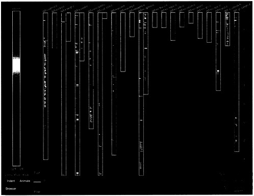
Figure 1. A SeeSoftTM display showing a module with 20 files and 9,365 lines of code. Each file is represented as a column and each line of code as a colored row. The newest rows are in red and the oldest in blue, with a color spectrum in between. This overview highlights the largest files and program control structures, while the color shows relationships between files, as well as unstable, frequently changed code. Eick et al. (1992b).
Much of the difficulty of software testing is in the management of the testing process (producing reports, entering MRs, documenting MRs cleared, and so on), the management of the objects of the testing process (test cases, test drivers, scripts, and so on), and the management of the costs and time of testing.
Typically, software testing refers to the phase of testing carried out after parts of code are written so that individual programs or modules can be compiled. This phase includes unit, integration, system, product, customer, and regression testing. Unit testing occurs when programmers test their own programs, and integration testing is the testing of previously separate parts of the software when they are put together. System testing is the testing of a functional part of the software to determine whether it performs its expected function. Product testing is meant to test the functionality of the final system. Customer testing is often product testing performed by the intended user of the system. Regression testing is meant to assure that a new version of a system faithfully reproduces the desirable behavior of the previous system.
Besides the stages of testing, there are many different testing methods. In white box testing, tests are designed on the basis of detailed architectural knowledge of the software under test. In black box testing, only knowledge of the functionality of the software is used for testing; knowledge of the detailed architectural structure or of the procedures used in coding is not used. White box testing is typically used during unit testing, in which the tester (who is usually the developer who created the code) knows the internal structure and tries to exercise it based on detailed knowledge of the code. Black box testing is used during integration and system testing, which emphasizes the user perspective more than the internal workings of the software. Thus, black box testing tries to test the functionality of software by subjecting the system under test to various user-controlled inputs and by assessing its resulting performance and behavior.
Since the number of possible inputs or test cases is almost limitless, testers need to select a sample, a suite of test cases, based on their effectiveness and adequacy. Herein lie significant opportunities for statistical approaches, especially as applied to black box testing. Ad hoc black box testing can be done when testers, perhaps based on their knowledge of the system under test and its users, decide specific inputs. Another approach, based on statistical sampling ideas, is to generate test cases randomly. The results of this testing can be analyzed by using various types of reliability growth curve models (see "Assessment and Reliability" in Chapter 4 ). Random generation requires a statistical distribution. Since the purpose of black box testing is to simulate actual usage, a highly recommended technique is to generate test cases randomly from the statistical distribution needed by users, often referred to as the operational profile of a system.
There are several advantages and disadvantages to statistical operational profile testing. A key advantage is that if one takes a large enough sample, then the system under test will be tested in all the ways that a user may need it and thus should experience fewer field faults. Another advantage of this method is the possibility of bringing the full force of statistical techniques to bear on inferential problems; that is, the results obtained during testing can be generalized to make inferences about the field behavior of the system under test, including inferences about the number of faults remaining, the failure rate in the field, and so on.
In spite of all these advantages, statistical operational profile testing in its purest form is rarely used. There are many difficulties; some are operational and others are more basic. For example, one can never be certain about the operational profile in terms of inputs, and especially
in terms of their probabilities of occurrence. Also, for large systems, the input space is high-dimensional. Thus, another problem is how to sample from this high-dimensional space. Further, the distribution is not static; it will, in all likelihood, change over time as new users exercise the system in unanticipated ways. Even if this possibility can be discounted, questions remain about the efficiency of statistical operational profile testing, which can be very inefficient, because most often the system under test will be used in routine ways, and thus a randomly drawn sample will be highly weighted by routine operations. This high weighting may be fine if the number of test cases is very large. But then testing would be very expensive, perhaps even prohibitively so. Therefore, testers often adopt some variant of drawing a random sample; for example, testers give more weight to boundary values—those values around which the system is expected to change its behavior and therefore where faults are likely to be found. This and other clever strategies adopted by testers typically result in a testing distribution that is quite different from the operational profile. Of course, in such a case the results of the testing laboratory will not be generalizable unless the relationships between the two distributions are taken into account.
Thus, to take advantage of the attractiveness of operational profile testing, some key problems have to be solved:
-
How to obtain the operational profile,
-
How to sample according to a statistical distribution in high-dimensional space, and
-
How to generalize results obtained in the testing laboratory to the field when the testing distribution is a variant of the operational profile distribution.
All of these questions can be dealt with conceptually using statistical approaches.
For (1), a Bayesian elicitation procedure can be envisioned to derive the operational profile. This elicitation is done routinely in Bayesian applications, but because the space is very high dimensional, techniques are needed for Bayesian elicitation in very high dimensional spaces.
Concerning (2), if the joint distribution corresponding to the operational profile is known, schemes can be used that are more efficient than simple random sampling schemes. Simple random sampling is inefficient because it typically gives higher probability to the middle of a distribution than to its tails, especially in high dimensions. A more efficient scheme would sample the tails quickly. This can be accomplished by stratifying the support of the distribution.
McKay et al. (1979) formalized this idea using Latin hyper cube sampling. Suppose we have a K-dimensional random vector X = (X1,...,XK ) and we want to get a sample of size N from the joint distribution of X.If the components of X are independent, then the scheme is simple, namely:
-
Divide the range of each component random variable in N intervals of equal probability,
-
Randomly sample one observation for each component random variable in each of the corresponding N intervals, and finally
-
Randomly combine the components to create X .
Stein (1987) showed that this sampling scheme can be substantially better than simple random sampling. Iman and Conover (1982) and Stein (1987) both discussed extensions for
nonindependent component variables. Of course, if specifying homogenous strata is possible, it should be done prior to applying the Latin hyper cube sampling method to increase the overall effectiveness of the sampling scheme.
Example : Consider a software system controlling the state of an air-to-ground missile. The key inputs for the software are altitude, attack and bank angles, speed, pitch, roll, and yaw. Typically, these variables are independently controlled. To test this software system, combinations of all these inputs must be provided and the output from the software system checked against the corresponding physics. One would like to generate test cases that include inputs over a broad range of permissible values. To test all the valid possibilities, it would be reasonable to try uniform distributions for each input. Suppose we decide upon a sample of size 6. The corresponding Latin hyper cube design is easily constructed by dividing each variable into six equal probability intervals and sampling randomly from each interval. Because we have independent random variables here, the final step consists of randomly coupling these samples. The design is difficult to visualize in more than two dimensions, but one such sample for attack and bank angles is depicted in Figure 2 . Note that there is exactly one observation in each column and in each row, thus the name "Latin hyper cube."
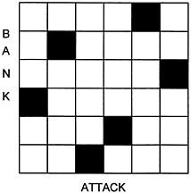
Figure 2. Latin hyper cube. N = 6 and K = 2.
Finally, concerning (3), to make inferences about field performance, the issue of the discrepancy between the statistical operational profile and the testing distribution must be addressed. At this point, a distinction can be made between two types of extrapolation to field performance of the system under test. It is clear that even if the true operational profile distribution is not available, to the extent that the testing distribution has the same support as the operational profile distribution, statistical inferences can be made about the number of remaining faults. On the other hand, to extrapolate the failure intensity from the testing laboratory to the field, it is not enough to have the same support; rather, identical distributions are needed. Of course, it is unlikely that after spending much time and money on testing, one would again test with the statistical operational profile. What is needed is a way of reusing the information generated in the testing laboratory, perhaps by a transformation in which some statistical techniques based on reweighting can help. There are two basic ideas, both relying heavily on the assumption that the testing and the field-use distributions have the same support. One idea is to use all the data from the testing laboratory, but with added weights to change the sample to resemble a random sample from the operational profile. The approach is similar to reweighting in importance sampling. Another idea is to accept or reject the inputs used in testing with a probability distribution based on the operational profile. For a description of both of these techniques, see Beckman and McKay (1987).
In his presentation at the panel's forum, Phadke (1993) suggested another set of statistical techniques, based on orthogonal arrays, for parsimonious testing of software. The example described above proves useful in an elaboration.
Example. For the software system that determines the state of an attack plane, let us assume that interest centers on testing only two conditions for each input variable. This situation arises, for example, when the primary interest lies in boundary value testing. Let the lower value be input state 0 and the upper value be input state 1 for each of the variables. Then in the language of statistical experimental design, we have seven factors, A,...,G (altitude, attack angle, bank angle, speed, pitch, roll, and yaw), each at two levels (0,1). To test all of the possible combinations, one would need a complete factorial experiment, which would have 27 = 128 test cases consisting of all possible sequences of 0's and 1's. For a statistical experiment intended to address only main effects, a highly fractionated factorial design would be sufficient. However, in the case of software testing, there is no statistical variability and little or no interest in estimating various effects. Rather, the interest is in covering the test space as much as possible and checking whether the test cases pass or fail. Even in this case, it is still possible to use statistical design ideas. For example, consider the sequence of test cases given in Table 2. This design requires 8 test cases instead of 128. In this case, since there is no statistical variation, main effects do not have any practical meaning. However, looking at the pattern in the table, it is clear that all possible combinations of any two pairs are covered in a balanced way. Thus, testing according to this design will protect against any incorrect implementation of the code involving a pairwise interaction.
Table 2a. Orthogonal array. Test cases in rows. Test factors in columns.
|
|
A |
B |
C |
D |
E |
F |
G |
|
1 |
0 |
0 |
0 |
0 |
0 |
0 |
0 |
|
2 |
0 |
0 |
0 |
1 |
1 |
1 |
1 |
|
3 |
0 |
1 |
1 |
0 |
0 |
1 |
1 |
|
4 |
1 |
1 |
1 |
1 |
1 |
0 |
0 |
|
5 |
1 |
0 |
1 |
0 |
1 |
0 |
1 |
|
6 |
1 |
0 |
1 |
1 |
0 |
1 |
0 |
|
7 |
1 |
1 |
0 |
0 |
1 |
1 |
0 |
|
8 |
1 |
1 |
0 |
1 |
0 |
0 |
1 |
Table 2b. Combinatorial design. Test cases in rows. Test factors in columns.
|
|
A |
B |
C |
D |
E |
F |
G |
|
1 |
0 |
0 |
0 |
0 |
0 |
0 |
0 |
|
2 |
1 |
1 |
1 |
1 |
1 |
1 |
0 |
|
3 |
0 |
0 |
1 |
1 |
1 |
0 |
1 |
|
4 |
1 |
0 |
0 |
0 |
1 |
1 |
1 |
|
5 |
1 |
1 |
1 |
0 |
0 |
0 |
1 |
|
6 |
0 |
1 |
0 |
1 |
0 |
1 |
1 |
In general, following Taguchi, Phadke (1993) suggests orthogonal array designs of strength two. These designs (a specific instance of which is given in the above example) guarantee that all possible pairwise combinations will be tried out in a balanced way. Another approach based on combinatorial designs was proposed by Cohen et al. (1994). Their designs do not consider balance to be an overriding design criterion, and accordingly they produce designs with smaller numbers of required test cases. For example, Table 2b contains a combinatorial design with complete pairwise coverage in six runs instead of the eight required by orthogonal arrays (Table 2a). This notion has been extended to notions of higher-order coverage as well. The efficacy of these and other types of designs has to be evaluated in the testing context.
Besides the types of testing discussed above, there are other statistical strategies that can be used. For example, DeMillo et al. (1988) have suggested the use of fault insertion techniques. The basic idea is akin to capture-recapture sampling in which sampled units of a population (usually wildlife) are released and inverse sampling is done to estimate the unknown population size. The MOTHRA system built by DeMillo and his colleagues implements such a scheme. While there are many possible sampling schemes (Nayak, 1988), the difficulty with fault insertion is that the faults inserted ought to be subtle enough so that the system can be compiled and tested; no two inserted faults should interact with each other; and while it may be possible at the unit testing level, it is prohibitively expensive for integration testing. It should be pointed out that the use of capture-recapture sampling, outlined in this chapter's subsection titled ''Design," for quantifying document reviews does not require fault seeding and, accordingly, is not subject to the above difficulties.
Another key problem in testing is determining when there has been enough testing. For unit testing where much of the testing is white box and the modules are small, one can attempt to check whether all the paths have been covered by the test cases, an idea extended substantially by Horgan and London (1992). However, for integration and system testing, this particular approach, coverage testing, is not possible because of the size and the number of possible paths through the system. Here is another opportunity for using statistical approaches to develop a theory of statistical coverage. Coverage testing relates to deriving methods and algorithms for
generating test cases so that one can state, with a very high probability, that one has checked most of the important paths of the software. This kind of methodology has been used with probabilistic algorithms in protocol testing, where the structure of the program can be described in great detail. (A protocol is a very precise description of the interface between two diverse systems.) Lee and Yanakakis (1992) have proposed algorithms whereby one is guaranteed, with a high degree of probability, that all the states of the protocols are checked. The difficulty with this approach is that the number of states becomes large very quickly, and except for a small part of the system under test, it is not clear that such a technique would be practical (under current computing technology). These ideas have been mathematically formalized in the vibrant area of theorem checking and proving (Blum et al., 1990). The key idea is to take transforms of programs such that the results are invariant under these transforms if the software is correct. Thus, any variation in the results suggests possible faults in the software. Blum et al. (1989) and Lipton (1989), among others, have developed a number of algorithms to give probabilistic bounds on the correctness of software based on the number of different transformations.
In all of the several approaches to testing discussed above, the number of test cases can be extraordinarily large. Because of the cost of testing and the need to supply software in a reasonable period of time, it is necessary to formulate rules about when to stop testing. Herein lies another set of interesting problems in sequential analysis and statistical decision theory. As pointed out by Dalal and Mallows (1988, 1990, 1992), Singpurwalla (1991), and others, the key issue is to explicitly incorporate the economic trade-off between the decision to stop testing (and absorb the cost of fixing subsequent field faults) and the decision to continue testing (and incur ongoing costs to find and fix faults before release of a software product). Since the testing process is not deterministic, the fault-finding process is modeled by a stochastic reliability model (see Chapter 4 for further discussion). The opportune moment for release is decided using sequential decision theory. The rules are simple to implement and have been used in a number of projects. This framework has been extended to the problem of buying software with some sort of probabilistic guarantee on the number of faults remaining (Dalal and Mallows, 1992). Another extension with practical importance (Dalal and McIntosh, 1994) deals with the issue of a system under test not having been completely delivered at the start of testing. This situation is a common occurrence for large systems, where in order to meet scheduling milestones, testing begins immediately on modules and sets of modules as they are completed.


