(NAS Colloquium) Earthquake Prediction: The Scientific Challenge (1996)

This paper was presented at a colloquium entitled “Earthquake Prediction: The Scientific Challenge,” organized by Leon Knopoff (Chair), Keiiti Aki, Clarence R.Allen, James R.Rice, and Lynn R.Sykes, held February 10 and 11, 1995, at the National Academy of Sciences in Irvine, CA.

J.S.LANGER*, J.M.CARLSON†, CHRISTOPHER R.MYERS‡, AND BRUCE E.SHAW§

*Institute for Theoretical Physics and †Department of Physics, University of California, Santa Barbara, CA 93106; ‡Center for Theory and Simulation in Science and Engineering, Cornell University, Ithaca, NY 14853; and §Lamont-Doherty Earth Observatory, Columbia University, Palisades, NY 10964

ABSTRACT We summarize recent evidence that models of earthquake faults with dynamically unstable friction laws but no externally imposed heterogeneities can exhibit slip complexity. Two models are described here. The first is a one-dimensional model with velocity-weakening stick-slip friction; the second is a two-dimensional elastodynamic model with slip-weakening friction. Both exhibit small-event complexity and chaotic sequences of large characteristic events. The large events in both models are composed of Heaton pulses. We argue that the key ingredients of these models are reasonably accurate representations of the properties of real faults.

Fault models of the kind pioneered by Burridge and Knopoff (1) (BK), with fully inertial dynamics but without externally imposed heterogeneities or stochastic perturbations, are deterministically chaotic systems whose behavior resembles that of real seismic sources (2–5). Like real faults, these models exhibit broad distributions of slipping events (i.e., earthquakes), including a range of small to moderately large localized events, which satisfy Gutenberg-Richter-like statistics, and large characteristic events, which dominate the cumulative slip. The individual events exhibit complex patterns of slip, and the large events are composed of narrow slip pulses—i.e., Heaton pulses. Many insights can be gained by studying the analogs of various seismic phenomena as they appear in such models. Because quantitative models provide the opportunity to track the evolution of faults with perfect accuracy and for arbitrarily long periods of time, these studies may ultimately lead to progress in areas such as seismic reconstruction and earthquake prediction.

Many different models of fault dynamics are currently being investigated. These include quasistatic three-dimensional continuum elastic models, one- and two-dimensional continuum models with inertial dynamics such as those we describe here, and cellular automata. In addition, existing models involve a wide variety of descriptions of the accumulation of stress as the system is loaded and the release and redistribution of stress during slip. While automata facilitate rapid numerical computation, continuum models have the advantage of allowing more direct associations to be made between model parameters—characteristic length and time scales, elastic constants and the like—and observations of real seismic phenomena.

Unlike the situation in fluid dynamics where the Navier-Stokes equation provides an agreed-upon description of the underlying physics, there is still no general consensus about what is the right model or equation for describing the motions of earthquake faults. Therefore, it is useful to study a variety of models and, in doing so, to learn how their various ingredients determine the behaviors that they exhibit. Of course, it is the modeler’s responsibility to be sure that the ingredients of a model provide a reasonable approximation to the system of interest and that observed properties are not artifacts of unphysical assumptions. An interesting feature that many fault models share with an emerging set of other strongly nonlinear nonequilibrium phenomena is that the physics at short length scales can sensitively determine behavior at the largest scales. For that reason, in using continuum models, particular care must be taken to extract continuum behavior from numerical approximations. This point has been emphasized recently by Rice and coworkers (6).

In this paper, we describe our studies of two particular versions of the BK model and discuss the degree to which various features of these models do, or do not, correspond to properties of the real world. We pay particular attention to the nature of the dynamic stick-slip instability, which is responsible for the complex patterns of events that these models exhibit. First, we describe the simple one-dimensional BK model with velocity-weakening friction. This is very nearly the same slider-block model that was introduced by Burridge and Knopoff in 1967, the main difference being that our version is completely uniform; all blocks have the same mass, and all spring constants and friction laws are independent of position and time. Second, we report some recent results obtained using a two-dimensional, crustal-plane model with slip-weakening friction.

We find it easiest to describe the uniform, one-dimensional, BK model by a massive wave equation with a slow driving force and velocity-weakening stick-slip friction. In dimensionless variables, this differential equation has the form

[1]

Here, U(x, t) is the displacement of an infinitesimal mass element or block at position x and time t. Dots denote time derivatives. The original BK slider-block model may be recovered by evaluating the displacement field U(x, t) on a discrete set of points along the x axis and making a finite-difference approximation for the spatial derivatives on the right-hand side of the equation.

The first term on the right-hand side of Eq. 1 is the linear elastic interaction between the blocks—that is, the force due to the nearest-neighbor coupling springs in the original BK model. The coefficient of this term (unity in our units) is a wave speed that may be identified as the velocity of elastic waves on the fault surface. The massive term, −(U−vt), is the force exerted by the BK leaf springs, which connect the blocks to a rigid plate moving at the loading speed v. We interpret this term as the coupling between the seismogenic layer and the

stably creeping lower region of the fault. The period of simple harmonic motion associated with this term is proportional to the time required for an elastic wave to traverse the crust depth, which is the same as the characteristic duration of slip at a single point on the fault in a very large, characteristic event. For real faults, this period is the order of seconds, the wave speed is the order of 10 kilometers/sec, and the corresponding length scale is the order of 10 kilometers. Accordingly, our unit of position x is this seismogenic depth.

The last term in Eq. 1 is the velocity-weakening stick-slip friction, which we usually have taken to have the form

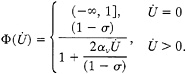
[2]

(For some applications, we have found piecewise linear or exponential forms of the velocity-weakening function to be more convenient. The qualitative properties of the model seem to be insensitive to the specific functional form of Φ.) We have chosen the slipping threshold to be unity by scaling U so that this threshold is reached in a completely uniform system when the displacement U is equal to −1 for all x. Thus our displacements U are measured in units of the characteristic slip in a very large event, a length of order meters for real faults. With this scaling, the dimensionless loading rate v is the ratio of the true loading rate, centimeters per year, to the characteristic slipping speed, meters per second. Therefore, v≈10⁻⁸.

Note that Eq. 2 is a specially simple friction law with a sharply defined slipping threshold and no extra rate or state dependencies (7, 8). This friction law permits no stable creep at small velocities, and the slipping threshold is fully restored immediately upon resticking.

The only important system-dependent parameter in this model is the velocity-weakening rate α_v, which cannot be measured directly in the Earth. In the absence of information to the contrary, we assume that α_v must have a value of order unity. The dynamic instability associated with the velocity-weakening force law is the principal cause of slip complexity in this system. A larger value of α_v means less energy dissipation and stronger instability; smaller α_v means more dissipation and weaker instability. We can see this explicitly from a simple linear analysis of the first-order displacement δU(x, t) during a slipping motion. Let δU~exp(ikx+ωt), where k is a wavenumber and ω is the amplification rate. Then, from Eqs. 1 and 2 we find that

[3]

This instability persists—ω remains positive—down to arbitrarily small wavelengths. As a result, the model needs some sort of short-wavelength cutoff. We shall return to this point.

The parameter σ that appears in Eq. 2 is the force drop or, equivalently, the acceleration of a block at the instant when slipping begins. We have introduced α in this version of the model primarily as a technical device that allows us to study the limit v → 0. In the absence of σ, events begin infinitely slowly in that limit, which obviously is inconvenient for numerical purposes. With a value of σ of order 10⁻² and vanishingly small v, on the other hand, we need not carry out explicit time integrations between slipping events and thus can study the system for very large numbers of loading cycles. We shall see, however, that σ has greater physical significance in the two-dimensional slip-weakening model.

We have performed numerical integrations of the equation of motion Eq. 1 over the equivalent of many thousands of seismic loading cycles with systems containing thousands of blocks. Our most important observation is that, in this limit in which the loading rate v is very small, the system exhibits persistent slip complexity. That is, if we start with any slightly nonuniform configuration U(x, t=0) and integrate Eq. 1 forward in time, without introducing any further noise or irregularities, we find chaotic motion. A portion of one such simulation is illustrated in Fig. 1, where we plot a sequence of fully stuck configurations. The displacements U(x) jump forward during slipping events, and the areas swept out by these events are our dimensionless seismic moments, M=∫δUdx.

Our extensive numerical studies indicate that what we are seeing in Fig. 1 is a finite sequence of configurations that belongs to a statistically stationary distribution of event sizes. Stationarity means that, after initial transients have disappeared, this distribution is entirely independent of the initial configuration. For α_v≥2, the distribution contains two distinct populations: a region of small to moderately large localized events (corresponding to the smaller events that cluster in the local minima in Fig. 1) that obey something like a Gutenberg-Richter (GR) law; and a region of large delocalized events—irregularly recurring characteristic earthquakes—whose frequency exceeds that of the extapolated GR law, and that account for essentially all of the moment release.

A typical frequency-magnitude distribution is shown in Fig. 2. Here, R(μ) is the differential distribution of frequencies of events of magnitude μ=lnM. The distribution of localized events in this log-log plot has slope −1, a value which persists for all α_v>2. For smaller α_v, we find smaller slopes; and we also find that, although complexity persists, the characteristic-event peak disappears near α_v=1 as the instability becomes weaker.

The large, delocalized events consist of pairs of slipping pulses that emerge from a nucleation zone and propagate in opposite directions along the fault at roughly the elastic wave speed. We have studied these Heaton pulses (9) in considerable analytic detail (10, 11) and find that they behave in many respects like shock fronts whose widths are controlled by the short-wavelength cutoff. The anomalous sharpness of these pulses may be an important factor in generating the small-event complexity that is seen in these models. The crossover between localized and delocalized events occurs at an event size that is proportional to the crust depth multiplied by an amplification factor (order of 2 or 3 for the parameters used

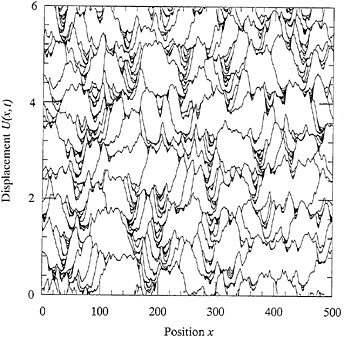
FIG. 1. Sequence of fully stuck configurations U(x) during a portion of a simulation of fault motion for the one-dimensional BK model.

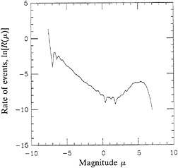
FIG. 2. Differential magnitude-frequency distribution for the one-dimensional velocity-weakening model with α_v=3.0, σ=0.01, and discretization length α=0.1.

here) that also depends (logarithmically) on the short-wavelength cutoff. Thus, the GR law extends up to events so large that their spatial extents are of the order of the crust depth or more.

Several ingredients of this model are sufficiently unorthodox or controversial that they require further comment. There is, of course, no experimental justification or theoretical rationale for the velocity-weakening friction law; but any attempt to model the dynamics of real earthquake faults at slipping speeds of the order of meters per second is necessarily speculative given our present state of understanding of these complex systems. More immediate issues pertain to the role of the short-wavelength cutoff and the role of elastodynamics in higher dimensions. Another important issue is the coupling to the bottom of the seismogenic layer—i.e., the −U term— which is best discussed later in connection with the two-dimensional model.

The need for a short-wavelength cutoff in Eq. 1 has raised the concern that complexity in this model might be an artifact of the numerical discretization rather than the result of inertial dynamics (12). To test this possibility, we have added a viscous

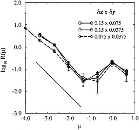
FIG. 3. Differential magnitude-frequency distributions for the two-dimensional slip-weakening model with α_s=3.0, σ=0.03, and τ=0.2. The three curves differ only in their grid spacings as shown. The system has size L_x=60, L_y=3.75. We have imposed periodic boundary conditions in the x direction and have added a layer of viscous damping at large y in order to minimize the effect of elastic waves being reflected back onto the fault from the boundary at y=L_y. The solid line has slope −1.

force, to the right-hand side of Eq. 1, and have repeated the numerical analysis with various values of the discretization length (13). With this new term, the linear dispersion relation analogous to Eq. 3 becomes

[4]

so that there is now a largest unstable wavevector, . If slip complexity were a result of some inherent discreteness in this model, it should disappear when the discretization length a becomes so small that k_ηa≪1. That does not happen. Complex, earthquake-like dynamics persists in this limit, and the frequency-magnitude distribution remains invariant throughout both the GR region and the region of large delocalized events. We also have looked analytically at propagating pulses in the model with viscosity and have examined the crossover from control by the grid size to control by the viscous length as the grid size becomes small (11). Again, we conclude that the continuum limit is perfectly well defined in this model and that slip complexity is an intrinsic feature of its inertial dynamics.

A specially important element that is missing in the one-dimensional models is the elastodynamics of the crust. To begin to address this issue, we recently have completed studies of a two-dimensional, crustal-plane version of the Burridge-Knopoff model in which a scalar displacement field U(x, y, t) satisfies a massive wave equation throughout a half plane, y> 0, bounded by the fault line which we take to be the x axis. Specifically,

As before, the −U term introduces a small-frequency, long-wavelength cutoff associated with the crust depth. The stick-slip friction Φ enters as a traction acting on the crustal plane at the fault

[6]

In our two-dimensional work so far, we have used a slip-weakening analog of Eq. 2 that is based on a frictional-heating model originally proposed by Sibson (14) and developed more recently by Lachenbruch (15) and Shaw (16). We write this failure law in the form

[7]

with

[8]

Here, S(x, t)=U(x, 0, t) is the displacement of the crust along the fault; S₀(x)=U[x, 0, t₀(x)] is the value of S at the beginning of an event; and t₀(x) is the time at which slip starts at the point x. Note that S(x) −S₀(x) is the total slip at x starting from the beginning of an event. In a complex event, the material at x may slip and restick more than once, but ϕ continues to decrease throughout this motion. When the event ends, the fault reheals instantly, and the slipping threshold is reset to ϕ(0)=1 everywhere.

Because this is a two-dimensional elastodynamic system, we cannot use the abrupt initial stress drop σ that we introduced in Eq. 2. Instead, in Eq. 7 the initial stress drops sharply but continuously over a time τ via the function

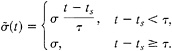
[9]

The time t—t_s is measured from the last unsticking at t_s so that, unlike S₀ or ϕ, is reset during an event if the fault resticks and then slips again. That is, the threshold for slipping during an event is the current value of ϕ increased by σ. The overall role of the stress drop in this model does require further investigation. In future work, we plan to use what we believe would be realistically larger values of σ and to replace the time-dependent form (Eq. 9) with a slip-dependent function that would provide a more realistic model of fracture at the onset of an event.

The analog of the linear dispersion relation (Eq. 3) for this model is obtained by writing δU ~ exp(ikx−Ky+ωt). We find

[10]

which implies that slipping deformations grow unstably for and that shorter wavelength perturbations propagate without either growing or decaying. As a result, we do not expect to need a short-wavelength cutoff in this model.

Our two-dimensional results (17) are remarkably similar to those that we found in one dimension. In Fig. 3 we show frequency-magnitude distributions for several different grid sizes. As in Fig. 2, we see a GR law with slope −1 for the smaller, localized events and an excess of large, delocalized events. For the smaller grid size, the GR law extends further in the direction of small (few-block) events; but the frequencies of the events at all larger magnitudes remain unaffected by this change in the numerics. We also see Heaton pulses as shown in Fig. 4. Finally, in Fig. 5, we show a scatter graph of individual events in the M, ∆ plane, where M is the seismic moment defined previously and A is the size of the slipping region along the x axis. For the localized events, we find that M scales roughly as σ∆2, consistent with the assumption of a constant stress drop of order σ in a two-dimensional system. For the delocalized events, on the other hand, M scales linearly with ∆ as we would expect for propagating pulses. Note that the initial stress drop σ sets the scale for the small events in this model and therefore is an essential ingredient of the failure mechanism.

As has been emphasized by Knopoff (18), the −U term in Eqs. 1 and 5 is inconsistent with Hookean elasticity; static stress fields decay exponentially and elastic waves become unphysically dispersive at long wavelengths. Our reply to this concern is that −U is a physically essential restoring force

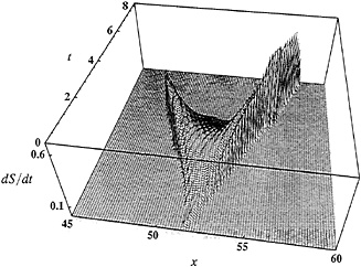
FIG. 4. Slip rate S as a function of position x and time t during a large event. Both pulses accelerate to approximately the wave speed (unity).

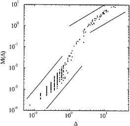
FIG. 5. Moment M as a function of slip zone size ∆. Dots indicate individual events. The lower two dashed lines have slope 2; the upper two lines have slope 1.

acting in response to motions of the seismogenic layer that take place in times the order of seconds or less. This time scale must play an essential role in the dynamics of seismic sources; it must be included somehow, and the—U term is the natural way for doing so in low-dimensional models. In a three-dimensional model of a strike-slip fault, with fully three-dimensional elastodynamics, we believe that this time scale would appear as a low-frequency cutoff in the dispersion relation for Rayleigh modes on the seismogenic part of the fault surface. Another way of arriving at the—U approximation in a two-dimensional theory is to replace it by a term that looks the same at high frequencies but vanishes in the static limit. For example, a term of the form with τ a time of order minutes or longer, would have precisely the desired properties. It would then be necessary, however, to replace −vt in Eq. 5 by another loading mechanism, say, a boundary condition that the crust be moving at speed v at some large distance from the fault. But these are projects for the future.

In summary, both the one- and two-dimensional models described here have features—small-event complexity, chaotic sequences of characteristic events, Heaton pulses, etc.—that seem qualitatively similar to the behavior of real earthquake faults. [This conclusion, that deterministic inertial dynamics in a uniform fault model can produce slip complexity, is also supported at least in part by recent work of Madariaga and Cochard (19).] Although these models are far from being complete enough to predict sequences of events on real faults or on systems of interacting faults, they do provide some insights that may already be relevant to the problem of prediction. For example, artificial catalogs generated by these models are being used for testing and improving prediction algorithms of the kind introduced by Keilis-Borok and coworkers (20–22).

The major outstanding issue, however, is the one raised at the beginning of this essay—whether the ingredients of these models are sufficiently realistic that the results can be taken seriously. In our opinion, the principal outstanding uncertainty about these models is not the—U term or even the friction law but instead the extent to which the underlying origin of the complex behavior of real faults is captured by instabilities associated with inertial dynamics. An alternative hypothesis is that slip complexity in the real world is primarily the result of some quenched inhomogeneity associated with the complex geometry of real faults, and that inertial dynamics is of no more than secondary importance. Certainly, geometric disorder does extend over a broad range of scales in real faults, from irregularities on the fault surface to the complex geometry of fault networks. Indeed, spatial irregularity—in the sense of

strongly pinned and weakly pinned regions in U(x, t)—is a generic feature of the models we study. However, in our case, this irregularity is an intrinsic property of the dynamics, as opposed to some extrinsic property introduced by the modeler.

In this regard, our point of view is the opposite of that taken by Ben-Zion and Rice (6, 12, 23), who see no evidence in their calculations that slip complexity can be generated solely by nonlinear dynamics on smooth faults. They are able, however, to reproduce observed behaviors by making their models inherently discrete and/or heterogeneous. There are some fundamental differences between their calculations and ours. Ben-Zion and Rice use rate- and state-dependent friction laws that do not produce the strong instabilities at high slipping speeds that emerge from our velocity- or slip-weakening laws. Also, in the work that they have published to date, they use quasi-static approximations, whereas we must solve the equations of motion for fully inertial elastodynamics in order to see the instabilities that generate complexity.

We cannot claim to know which of these approaches ultimately will prove to be the more realistic and useful, but we do believe that the differences in friction and dynamics explain the discrepancies between our results and those of others. If the geometric complexity of real faults is the overwhelmingly most important source of slip complexity, then quasistatic models with externally imposed heterogeneities may be most useful for practical purposes. On the other hand, if intrinsically smooth faults are deterministically chaotic systems that generate their own irregularities during unstable slipping motions, then models of the sort that we have described here will be essential for progress in earthquake prediction.

The work of J.M.C. was supported by the David and Lucile Packard Foundation, National Science Foundation (NSF) Grant DMR-9212396, and a grant from Los Alamos National Laboratory. J.S.L. was supported by Department of Energy Grant DE-FG03–84ER45108 and NSF Grant PHY89–04035. C.R.M. was supported by NSF Grant ASC-9309833 and the Cornell Theory Center. B.E.S. was supported by NSF Grants 93–16513 and USC-569934.

1. Burridge, R. & Knopoff, L. (1967) Bull. Seismol Soc. Am. 57, 3411.

2. Carlson, J.M. & Langer, J.S. (1989) Phys. Rev. Lett. 62, 2632–2635.

3. Carlson, J.M. & Langer, J.S. (1989) Phys. Rev. A 40, 6470–6484.

4. Carlson, J.M., Langer, J.S., Shaw, B.E. & Tang, C. (1991) Phys. Rev. A 44, 884–897.

5. Carlson, J.M., Langer, J.S. & Shaw, B.E. (1994) Rev. Mod. Phys. 66, 657–670.

6. Rice, J.R. & Ben-Zion, Y. (1995) Proc. Natl. Acad. Sci. USA (1996) 93, 3811–3818.

7. Dieterich, J.H. (1981) in Mechanical Behavior of Crustal Rocks: The Handin Volume, Geophys. Monogr. Ser., ed. Carter, N.L. (Am. Geophys. Union, Washington, DC), Vol 24, pp. 108–120.

8. Ruina, A.L. (1983) J. Geophys. Res. 88, 10359.

9. Heaton, T.H. (1990) Phys. Earth Planet. Inter. 64, 1.

10. Langer, J.S. & Tang, C. (1991) Phys. Rev. Lett. 67, 1043–1046.

11. Myers, C.R. & Langer, J.S. (1993) Phys. Rev. E 47, 3048–3056.

12. Ben-Zion, Y. & Rice, J.R. (1993) J. Geophys. Res. 98, 14109.

13. Shaw, B.E. (1994) Geophys. Res. Lett. 21, 1983.

14. Sibson, R.H. (1973) Nature (London) 243, 66.

15. Lachenbruch, A. (1980) J. Geophys. Res. 85, 6097.

16. Shaw, B.E. (1996) J. Geophys. Res., preprint.

17. Myers, C.R., Shaw, B.E. & Langer, J.S. (1995) preprint.

18. Knopoff, L. (1995) Proc. Natl. Acad. Sci. USA 93, 3830–3837.

19. Madariaga, R. & Cochard, A. (1995) Proc. Natl. Acad. Sci. USA 93, 3819–3824.

20. Keilis-Borok, V. (1995) Proc. Natl. Acad. Sci. USA 93, 3748–3755.

21. Pepke, S., Carlson, J.M. & Shaw, B.E. (1994) J. Geophys. Res. 99, 6789.

22. Kossobokov, V.G. & Carlson, J.M. (1995) J. Geophys. Res. 100, 6431.

23. Rice, J.R. (1993) J. Geophys. Res. 98, 9885.