
2
Mission Scenarios and Measurement Techniques
The path of an Earth-orbiting satellite departs from a simple Keplerian ellipse because of various perturbing forces acting on the satellite. These include the effects of atmospheric drag and solar radiation pressure, in addition to the gravitational attractions of the Sun, Moon, and Earth. By observing the motion of a satellite one obtains information about the forces acting on it, including the anomalies in the Earth's gravity field. Models of the Earth's gravity field are combined with models of these other forces in order to predict the path of a satellite, and the predictions are compared against the observations. As observational data are refined the model parameters are adjusted, yielding improved gravity field models. The history of this process is shown in Table 1.1 of Chapter 1.
Two kinds of errors can be introduced into the estimated gravity field model during this force modeling process. The first might be said to introduce a "bias," or a "systematic error," or to affect the "accuracy" of the estimated gravity field. The second might be called a ''random error," or "noise," which limits the "precision" of the gravity field estimates. Both will affect how far an estimated gravity field model departs from the "true" gravity field of the Earth. The first kind of error occurs when there are systematic biases in the measured quantities, or when non-Earth-gravitational perturbations are erroneously attributed to the gravity field. These errors make the estimated gravity field model inaccurate. The second kind of error occurs because the quantities of interest can only be measured with a finite precision, and noise in the observations makes the estimated gravity field imprecise.
In this chapter we describe some scenarios for satellite missions that could improve our knowledge of the Earth's gravity field. Some of these involve mature technologies that are probably feasible now; others envision using emerging technologies that may be ready to fly at some time in the future. All are discussed in a generic form. The literature on specific missions proposed in the past or for the future gives more technical details, and is cited where appropriate. At the end of this chapter there is a table summarizing the generic mission scenarios referred to in the subsequent chapters.
We estimate the ability of each of our generic missions to resolve the gravity field using standard techniques in spherical harmonic analysis. Spherical harmonic analysis of functions defined at points on a sphere is analogous to Fourier analysis of functions defined at points on the real line. We use a convolution theorem and assumed statistical distributions to obtain relationships among mean square values averaged over the surface of a sphere, called "variances." The square roots of these quantities are the root-mean-square (rms) average values, which we call "amplitudes." A constituent of a function with harmonic degree l has a wavelength of 40,000 km/l. A graph of constituent variance or amplitude versus l is a "degree spectrum," analogous to the power and amplitude spectra of one-dimensional functions. We characterize the resolution capabilities in terms of the rms amplitude of the
uncertainty in an areal average of the gravity or geoid anomaly; we illustrate this as "precision" versus a "resolution," the latter being the square root of the area. Precisions have units of geoid height or gravity anomaly and resolutions have units of length. Degree amplitude spectra are dimensionless and represent the amplitude of a quantity relative to the total amplitude of the Earth's gravity field. Details of these methods are given in Appendix A.
Our characterization of the resolution of these generic missions is essentially an analysis of how the error in a measured quantity will map into an error in the gravity field model. As such, it is a study of errors of the second kind, that is, of the "precision" of the derived gravity field model. However, we also discuss what ancillary measurements are required in order to facilitate a correct modeling of the non-gravitational signals, so that type-one errors will be reduced or eliminated. These missions are expected to make a significant improvement in the gravity field at short wavelengths, that is, at frequencies of many cycles per revolution of the satellite orbit. Most of the nongravitational modeling errors are confined to frequencies of one or a few cycles per revolution, that is, at very long wavelengths where the gravity field is already well known. Thus a spectral separation of the two kinds of errors is also possible. In the chapters following this one, we will compare the size of gravity field signals associated with various scientific problems against the resolution and error estimates obtained here. In effect, this means that the "error" estimates obtained here are treated as though they were ''departure from the truth." This treatment is justified by the spectral separation noted above and in the later error analysis review. These have shown that by placing accelerometers and/or GPS receivers onboard the spacecraft, one obtains the necessary data to separate the gravitational and non-gravitational signals.
SATELLITE OBSERVATIONS OF THE GRAVITY FIELD
Since the beginning of the satellite era in 1957 the tracking of orbiting satellites has been done from sites on the surface of the Earth, first optically, and later by Doppler and laser techniques. In the 1980s, a new dimension was added to these methods with the development and maturation of GPS of the U.S. Department of Defense, and the Global Navigation Satellite System (GLONASS), developed by the former USSR. Both these systems involve a constellation of high altitude satellites broadcasting navigation information which may be used by a receiver to determine its position both accurately and precisely. Virtually continuous tracking data obtained from high-quality GPS receivers onboard the low-altitude Ocean Topography Experiment (TOPEX/Poseidon) and GPS Meteorology Satellite (GPS/MET) have proven valuable in improving the resolution of the currently available Earth gravity field models (Tapley et al., 1996a; Lemoine et al., 1996).
The accurate determination of the long-wavelength (few thousand kilometers and longer) components in current gravity field models is largely due to extensive satellite tracking data. Medium- and shorter-wavelength components are constrained by combining satellite tracking data with heterogeneous data sets of land and marine gravity anomaly surveys and satellite altimetry. A dedicated spaceborne gravity mapping mission has long been seen as the means to improve the accuracy and resolution of Earth gravity field models. Such a mission would provide data of global extent and homogeneous quality, without the geographic or geopolitical limitations of altimetry and surface gravity anomaly surveys.
Most of the mission scenarios we describe in this report would improve the sensitivity to the gravity field by using various forms of satellite-to-satellite tracking. These include both a "high-low" scenario, in which a low-altitude satellite tracks its position with respect to the high-altitude GPS and/or GLONASS systems, and "low-low" scenarios, in which two low-altitude satellites track one another's motions. In another category are the "gradiometer" missions, which measure spatial gradients (derivatives) of the gravity field. If the distance separating the two spacecraft in a low-low mission is small (a few hundred kilometers), the mission will be particularly sensitive to differences in gravity over that distance. Because differentiating a signal will amplify its short-wavelength components more than its long-wavelength components, both the low-low tracking and the gradiometer scenarios could yield enhanced resolution of gravity field components between a few hundred and a few thousand kilometers.
TRADE-OFFS IN SPACECRAFT MISSION DESIGN
The ability of a satellite-borne instrument to provide measurements of the anomalous gravity field of the Earth depends on its orbital altitude. This is due to the attenuation of the gravitational potential with altitude, shown in Figure 2.1 (top panel) and described
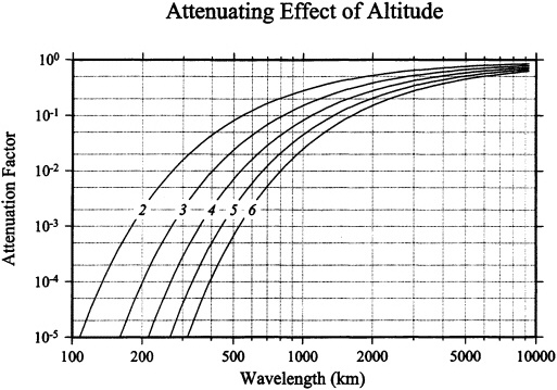

FIGURE 2.1 Top panel: The attenuation of gravitational potential with orbital altitude. Numbers labeled 2 through 6 denote orbital altitudes of 200 through 600 km, respectively. Bottom panel: The time required to acquire a ground-track pattern that will resolve a given across-track wavelength. Curves are drawn for the same orbital altitudes as in the top panel.
in Appendix A, section A.4. Most dedicated geopotential mapping mission scenarios call for low-altitude orbits (250 to 600 km) in order to maximize sensitivity to anomalies in the gravity field.
The altitude of the orbit is linked to the mission lifetime. The density of the atmosphere increases exponentially with decreasing altitude, so that the effect of the dissipative atmospheric drag accelerations becomes very significant at low altitudes. This drag will cause the orbital altitude to decay and eventually the satellite will re-enter the lower atmosphere, unless it is periodically boosted to a higher altitude by burning fuel carried onboard. The duration before re-entry, or the satellite mission lifetime, is dependent upon the initial altitude of injection, the ballistic characteristics of the satellite, the onboard fuel-carrying capacity, and the ambient drag conditions, which, in turn, depend upon the phase of the solar cycle. While predictions of orbit lifetime differ widely, in general satellites in the 250 to 350 km altitude range will last approximately 6 to 12 months in orbit, while those in 400 to 600 km altitude may last up to 2 to 5 years or more, depending upon the solar activity (Figure 2.2). Through these considerations, there are direct links between the observability of the geopotential, the mission's lifetime, the launch time table, and the weight and cost of the satellite.
At the range of altitudes discussed here, the spacecraft typically makes 15 to 16 revolutions of the Earth every day, at speeds of approximately 7.5 km per second. With measurements taken every few seconds, a dense sampling of the perturbative effects of the anomalous potential may be obtained along the satellite's ground track. The spatial sampling ability of any mission is thus limited by the across-track separation or the distance between two adjacent ground traces of the satellite's trajectory. Following Nyquist sampling requirements, resolution of an across-track anomaly of a given wavelength requires the satellite ground tracks

FIGURE 2.2
Orbit lifetime as a function of initial altitude and solar cycle. Polar circular orbits, A/M = 1 m2/77 kg. Computed by L.K. Newman, NASA Goddard Space Flight Center.
to be separated by half that wavelength or less. Thus an increase in the desired resolution requires a concomitantly denser sampling of the globe by the satellite ground tracks. However, this also means that the same geographical location can be sampled again only after a longer duration. Figure 2.1 (bottom panel) shows the acquisition time required to resolve a given across-track wavelength at the equator, where the track separation is largest. To resolve a spatial wavelength of λ the satellite must make at least 2l revolutions around the Earth, where l = 40,000 km/λ. At an orbital altitude of 400 km, the satellite makes 15.5 revolutions per day, and so the orbit repeat time R must be at least 80,000 km/15.5l days. Figure 2.1 (bottom panel) shows the trade-off between λ and R. An orbital repeat time of R limits the shortest period temporal oscillation that can be resolved to T= 2R. There is thus a trade-off between the spatial and temporal resolutions that might be obtained from an orbit design, such that the product Tλ is roughly 10,000 km-days. (While it might seem that l revolutions are sufficient to resolve degree l, in fact 2l are required [Jekeli and Rapp, 1980].)
The mission design also affects the science capability in other ways. To separate properly the time-varying gravitational effects from the static gravity field, it is necessary that a long record of measurements be available. An ideal mission design might call for low altitudes for desired high values of signal-to-noise ratios; long lifetimes to ensure adequate separation of the static and time-varying parts of the gravity field; and low weights to reduce launch and mission costs. These requirements are not all mutually compatible and potentially influence the science returns from a geopotential mapping mission. A mission flown continuously at altitudes below 300 km, as aspired to 15 years ago, becomes much more expensive because of the launch costs to put such mass in orbit. It now appears preferable that a satellite mission be placed at a higher altitude, where it would stay in orbit for several years, while resolving the longer wavelength components of the geopotential over that time scale, after which the natural decay of its orbit would allow it to resolve the shorter wavelengths over the last few months. As a further example, if the observing instrument must be cooled to superconducting temperatures, the current state of the technology limits the liquid helium dewar life, and hence the mission lifetime, to approximately 9 months. In such a case, it becomes necessary to fly at the lowest practical altitude, in order to maximize the resolution of the geopotential, while obtaining a snapshot (in time) of the gravity field.
MISSION SCENARIOS
GPS
The simplest concept for the mapping of the Earth's gravity field from space involves a single low altitude satellite, carrying a GPS or GLONASS receiver. Also onboard might be a high precision accelerometer, in order to properly model the effects of atmospheric and other non-gravitational accelerations upon the motion of the satellite. Failure to model these latter effects adequately will reduce the accuracy with which the geopotential models may be estimated from satellite tracking data. Such a scheme, making measurements of the satellite position, will be referred to hereafter as "GPS." Examples of such mission concepts are described in Reigber et al. (1996) and Clark et al. (1996).
SST and SSI
Another gravity-field-mapping scheme involves the measurement of the differences in satellite orbital perturbations over baselines of a few hundred kilometers (typically 100-600 km). These measurements may be made by placing two satellites in the same orbit but separated from each other by a few degrees, so that, in effect, one satellite "chases" the other. Mutual tracking between the two satellites then provides the information on the differential accelerations acting on the two satellites.
Two scenarios for making such measurements are considered in this report. In one, a microwave link between the two satellites is used to measure the line-of-sight range-rate (time derivative of the inter-satellite distance); this will be called Satellite to Satellite Tracking, "SST." In the other, the inter-satellite tracking is done using laser interferometry; hereafter called Satellite to Satellite Interferometry, or "SSI." Both these mission concepts are expected to carry high precision accelerometers at the center of mass of each of the satellites. This ancillary measurement is necessary to enable the effect of differential non-conservative accelerations on the inter-satellite orbit perturbations to be modeled accurately. Some examples of such missions are discussed by Fischell and Pisacane (1978), Pisacane et al. (1982), Yionoulis and Pisacane (1985), Keating et al. (1986), Bender (1992), Frey et al. (1993), Davis et al. (1996), and Chao et al. (1996).
Our SST mission scenario characterizes the current capabilities of a mature technology using a microwave sensor. Our SSI mission scenario envisions some
future engineering developments (e.g., reduction of thermal noise in the laser cavity), which might allow a laser to achieve an order of magnitude improvement in sensitivity over the current microwave design. The necessary developments are being studied as part of the European Space Agency's Cornerstone Project LISA, a laser interferometer space antenna intended to observe gravitational waves.
SGG and SGGE
When a satellite of finite extent is in orbit under the influence of purely gravitational accelerations, only its center of mass is in free fall. An accelerometer rigidly attached to such a satellite at a point displaced from the center of mass will measure only the acceleration relative to the center of mass. The difference in the acceleration measurements between two such collinear accelerometers, divided by the (short) baseline distance, yields a measurement of the gradient of gravitational acceleration along the baseline. This concept, extended to include three mutually orthogonal baselines (typically a few centimeters long) within the satellite, forms the basis of gravity gradiometry. Such a gravity gradiometer is likely to use a cryogenic super-conducting technology to ensure very high precisions of differential acceleration measurements. This concept is referred to hereafter as a Spaceborne Gravity Gradiometer, or "SGG." Examples of such mission concepts are described by Morgan and Paik (1989), European Space Agency (ESA) (1991, 1996), Rummel and Schwintzer (1994), and Bills and Paik (1996).
Current engineering constraints limit the time that a cryogenic SGG can be kept cold to something on the order of 9 to 12 months. It is conceivable that future technological advances will make it possible to operate an SGG for a much longer period of time. Such an extended SGG we refer to as "SGGE."
PREVIOUS STUDIES
The study of the capabilities and requirements of satellite gravity missions has a long history in the geodetic literature. These studies describe the signals in the various measurements, the nature of the principal error sources, and their effects on the resolution of the estimated gravity field. These error analyses have ranged from the approximate, rule of thumb techniques assuming white noise measurement errors, to fully rigorous numerical simulations of diverse random and systematic measurement and model errors.
The GPS mission concept is the only one for which real data have been analyzed and incorporated into a gravity field model. Two such examples are GPS tracking of TOPEX/Poseidon and GPS/MET satellites (Tapley et al., 1996a). The data from these satellites have been incorporated into the JGM3 (Tapley et al., 1996) and the EGM96 (Lemoine et al., 1996) models and have proven the value of high-density GPS tracking. Future GPS tracking missions should yield results that are enhanced by lower flight altitudes and will most likely carry an accelerometer to reduce the errors due to mismodeled non-gravitational accelerations. Several studies have been conducted on the use of the GPS concept for improvements in the gravity field models. Simulations for the Shuttle-GPS Tracking for Anomalous Gravitation Estimation experiment (Jekeli and Upadhyay, 1990) showed that 2-degree-mean anomalies could be estimated to 5 mGal. In the Aristoteles configuration (Schrama, 1991), tracking a Sun-synchronous satellite in a 250-km orbit yields a 1-mGal cumulative point-value error up to spherical harmonic degree 70 or so. The Polar Orbiting Platform Satellite-Geopotential Recovery Mission simulations (Reigber et al., 1987) showed errors ranging from 3 to 8 mGal depending on the duration of the mission. It is clear from all these results, however, that a gravity-mapping mission that includes only GPS tracking will not provide a "quantum leap" improvement in modeling the Earth's gravity field. Its most significant contribution would be at the longest wavelengths. In this sense it could be complementary to other gravity-mapping techniques.
The studies of SST missions have appeared in the literature in step with the various past proposals for such space missions. Early simulations focused on the Geopotential Research Mission scenario (Keating et al., 1986), using Fourier analysis of the inter-satellite range-rate signals (Kaula, 1983; Wagner, 1983) to determine that gravity field models of high degree and order could be resolved using this technique. Other studies (Douglas et al., 1980) used a local gravity inversion technique to show that with 1 µm/s range rate, the 1-degree-mean anomalies could be determined to near 1 mGal precision. All of these studies assumed satellite altitudes of 160 km, which required some form of drag compensation or frequent orbit maneuvers to raise the altitude for any reasonable mission lifetime.
Simulation studies of the gravity gradiometer mission concepts are more recent and have focused on ESA's Aristoteles mission scenario. This mission calls
for a gradiometer and a GPS receiver onboard the spacecraft. Consortium for Investigation on Gravity Anomaly Recovery (CIGAR) (1996) presents a review of the considerable literature devoted to this mission. Extensive study of a gradiometer mission with a 0.01 Eötvös (1 E = 10-9 s-2) precision has been made by the European geodetic community. Under the somewhat restrictive assumption of total loss of gradiometer signal at frequencies below 5 mHz (27 cycles per revolution) along a 200-km altitude Sun-synchronous orbit, Visser et al. (1994) showed that 100-km-mean anomalies could be recovered to 5 mGal or better from such a mission, with high-low GPS tracking playing an integral part in determining the long wavelength features of the gravity field.
Using an approximation based on white-noise measurement errors, Rapp (1989) showed that 1-degree-mean anomalies could be determined to 2, 3, and 5 mGal with mission altitudes of 160, 200, and 240 km, respectively. The corresponding precisions expected for 0.5-degree anomalies were 7, 9, and 11 mGal, respectively. Rummel and Schrama (1991) pointed out that the precisions at half-wavelengths less than 100 km would be approximately 1 mGal in the presence of white-noise measurement errors. CIGAR (1990) and Visser et al. (1994) showed that the effects of bandwidth limitations on measurements at frequencies less than 5 mHz and of polar data gaps due to the Sun-synchronous orbit are significant, and they recommended the use of GPS tracking and a priori constraint to reduce the estimation errors as well as to handle numerical instabilities in the data-inversion process. Kahn and von Bun (1985) pointed out that a 0.001-E instrument in a 160-km orbit could further improve the determinations of 0.5 degree mean anomalies to 3 mGal. Only a few rigorous numerical simulations of the gravity gradiometer problem have been carried out to high degree and order, due to limitations on computer time. Bettadpur (1993) reported supercomputer simulations to degree and order 100, taking into account orbit, white and colored measurement noise, and drag-mismodeling errors. He showed that the alignment of the sensitive axis of the accelerometer and the reduction of the accelerometer cross-talk factors were important for removing both the mean and the episodic (short-period) errors arising from variations in drag acceleration. The computing issues in gravity gradiometry were addressed by Balmino and Barriot (1991). A more comprehensive analysis of the Gravity Field and Steady-State Ocean Circulation Mission (ESA, 1996), based on a measurement accuracy of 0.001 E, addressed the need for an improved gravity field in such diverse areas as geodesy, geodynamics, oceanography, and orbit determination.
ERROR ESTIMATES FOR MISSION SCENARIOS OF THIS REPORT
All the mission concepts discussed here will yield observations with some limited precision. To determine definitive error estimates for a specific mission, it would be necessary to have a detailed engineering summary of the mission, including the spectra of all the errors, and to combine these with full numerical simulations of the estimation of the gravity field. Such a complete analysis is beyond the scope of this report. Instead, we make some simplifying assumptions that allow us to use analytical expressions to relate errors in the mission data to errors in the coefficients of the gravity field model. The error amplitudes we give are root-mean-square average values; that is, they are the square roots of the expected variances and may be thought of as "one-sigma" errors. Our approach and assumptions are outlined here; further details are in Appendix A.
Degree Amplitude Error Spectra
We begin with the assumption that the orbit will distribute errors in the observed quantity isotropically over the surface of a sphere surrounding the Earth at the altitude of the satellite orbit. In practice, no real orbit can distribute errors in this way; the ground track pattern is always least dense at the equator and most dense at the highest latitudes reached by the orbit. The actual orbits in real missions are likely to be very slightly elliptical and may be Sun-synchronous in order to simplify the design of the solar power systems. Sun-synchronicity requires the orbital plane to be inclined approximately 6 to 8 degrees from the polar axis so that small areas over the poles will not be covered by the satellite's ground track pattern. However, the assumption of isotropic error distribution permits us to convert the power spectral density (PSD) of the error in the time series of observables into the spatial covariance of the observable error over a sphere at satellite altitude. Once we have this, we can proceed with an error propagation analysis that treats the mean square values of errors averaged over a spherical surface. The error estimates we obtain by this method
will be average values; they may somewhat underestimate the errors at the equator and overestimate the errors at the maximum latitude reached by the satellite, and they will certainly underestimate the errors over polar gaps, if the orbit is not polar.
We used the method of Jekeli and Rapp (1980) to convert the PSD for errors in the time series of the observable into the spatial covariance of observable errors distributed over a sphere. This method assumes that the PSD of the errors is white. In reality, the data from an actual mission will likely have non-white PSDs, that is, correlated errors. We expect this to affect our error estimates primarily at the lowest degrees.
The Jekeli and Rapp method requires us to select a duration over which the data are analyzed, D. D must be chosen to be long enough that the assumption of spatially isotropic error distribution is justified. For example, if one wants to estimate the error in a spherical harmonic coefficient of degree l, then D must be long enough that the satellite makes at least 2l revolutions around the Earth during the time D. We chose D = 90 days. At the altitudes we simulated, a satellite makes about 15.6 revolutions per day and 1400 revolutions in 90 days; thus our calculations should be good to l = 700. We found that none of our simulated missions could resolve 1 > 300, so it would have been safe to have used any duration greater than about 40 days. Our resolution estimates for D = 90 can be rescaled to any D' > 40 by multiplying our resolved amplitudes by v(D/D') to obtain resolved amplitudes for a different duration. Later chapters discuss time variations in the gravity field and assume that a five-year mission can obtain an independent sample of the gravity field every D days.
The above process results in a covariance function for the errors in the observable that is distributed isotropically over the sphere at satellite altitude. Next, we make the assumption that all the forces on the satellite apart from the Earth's gravity field can be correctly modeled so that the signal in the observed quantity is caused entirely by the Earth's gravity field. This allows us to relate the covariance of the error in the observable at satellite altitude to the covariance of the errors in the coefficients of the gravity-field model. For the SGG and SGGE missions we need the spatial derivatives of the field (Appendix A, equation A.16), which are well known; an elegant so-called "Meissl Scheme" solution has been given by Rummel and van Gelderen (1995). We follow previous studies in making the approximation that the errors in the recovered gravity field can be estimated from the errors in the second radial gradient only. The SST and SSI missions need a relation involving the range-rate observable—this has been derived from an energy integral by Jekeli and Rapp (1980). This expression requires specification of the angular separation between the two spacecraft (d in equation A. 15 of Appendix A); we assumed a separation of two degrees. For the GPS case no analytic scheme was available, so we used the error predictions from numerical simulations for the white noise case reported by Bettadpur and Tapley (1996b). There, the observation data were assumed to be the double-differenced ranges between one ground receiver, one satellite receiver, and two GPS satellites. In practice, this would be derived from pair-wise differencing of the GPS carrier phase measurements between the two GPS satellites and the two receivers. The results from this study were appropriately scaled to reflect various altitude, noise level, and mission durations.
The white-noise levels we assumed for the missions were as follows: for the GPS mission, a 1 cm rms error in the double-difference range data. For the SST, a PSD of 0.5 (micron/s)/vHz in the microwave measurement of line-of-sight range-rate. For the SSI, a PSD of 0.05 (micron/s)/vHz in the interferometer measurement of line-of-sight range-rate. For the SGG and SGGE missions, we assumed that the error source was predominantly the error in the second radial-radial derivative of potential, and we assumed a PSD for this error of 0.001 E/vHz. These measurement-noise levels were chosen to yield gravitational parameter precisions that are representative of those expected from contemporary mission designs.
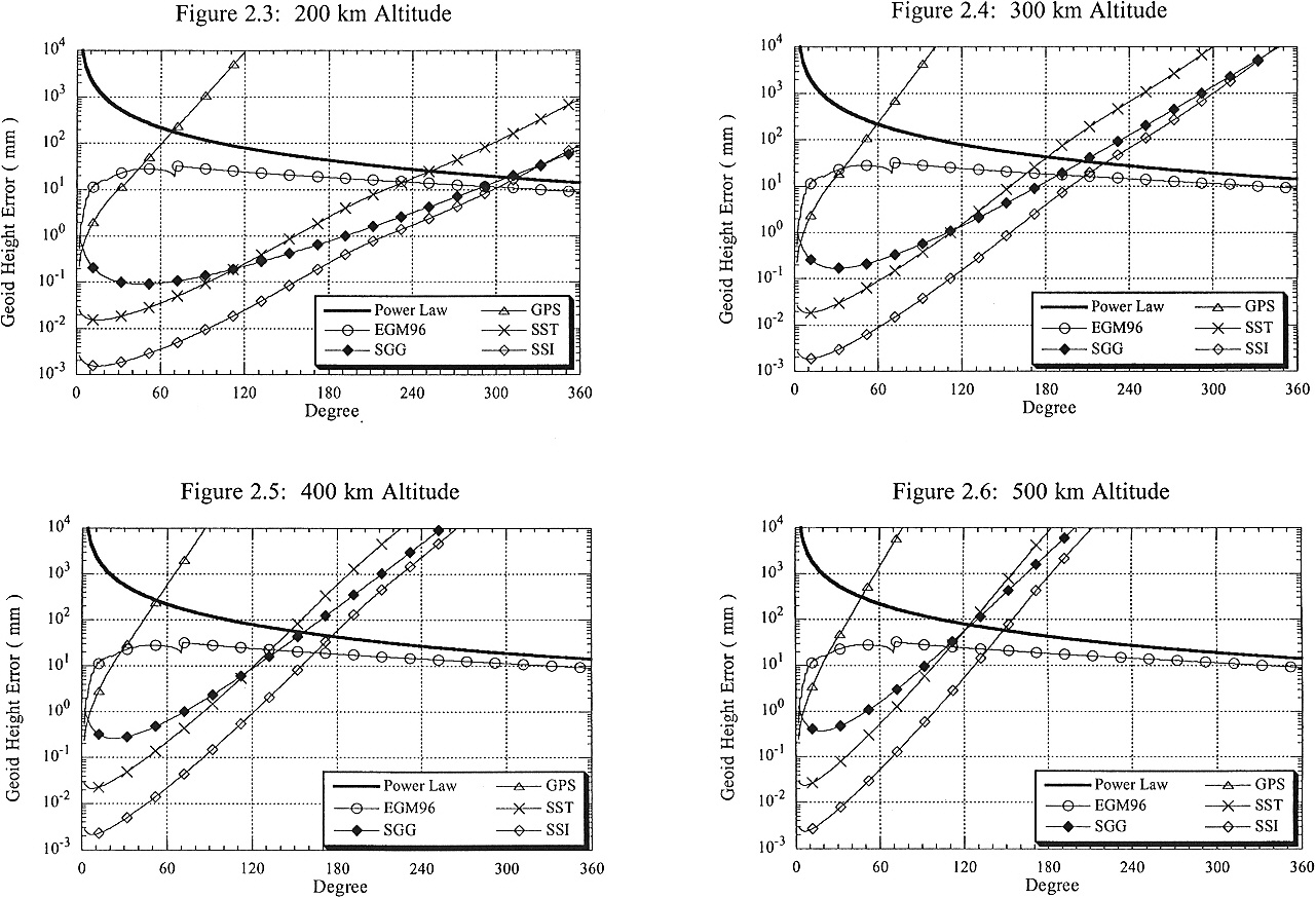
Figures 2.3-2.6 show the degree amplitude spectra (the rms amplitude of the errors in the geoid, sl) we obtained by this method for our GPS, SST, SSI, and SGG mission scenarios at altitudes of 200, 300, 400, and 500 km. Also shown are the error amplitudes for a current state-of-the-art gravity field model, EGM96 (Lemoine et al., 1996), reflecting the current status of knowledge based upon tracking data (predominately satellite laser ranging), surface gravity-anomaly measurements, and satellite altimetry. The figures show that a 90-day GPS mission provides an improvement over the current knowledge of the long-wavelength components of the mean gravity field, but the errors rise rapidly with increasing degrees. For a fixed altitude, the SST errors are lower than SGG errors at degrees less than 100 or so. The well-known insensitivity of SGG data to the long-wavelength geopotential is an inherent property of the gradient data type. We have not included the data from the onboard GPS receiver in our simulation for SGG. Had we done
so, the SGG error amplitudes at any degree would be approximately equal to the minimum of the SGG and GPS error amplitudes shown in Figures 2.3-2.6. Note that this would serve to reduce the errors in a gradiometer-derived gravity model at the low degrees where the GPS mission has smaller errors, though the resulting SGG+GPS errors would still be larger than the SST or SSI errors below degree 100. The SGG errors are smaller than SST errors at higher degrees. In all cases, the errors from SGG and SST become greater than the errors in current gravity models at degrees greater than 200 for missions at an altitude of 300 km, and degree 120 for the 500-km missions. Because the SSI is essentially an SST with an order-of-magnitude greater precision, it out-performs all the other missions. It would provide improved knowledge of the gravity field to harmonic degree 140-300, depending on its orbital altitude.
Precision Versus Resolution
We used the degree amplitudes in Figures 2.3-2.6 to derive resolution estimates that are more understandable physically. These are shown with a resolution length on the horizontal axis and a precision amplitude on the vertical axis: geoid-height precisions in Figures 2.7-2.10 and gravity-anomaly precisions in Figures 2.11-2.14. These precisions represent the expected (average behavior over the sphere) root-mean-square uncertainty (one sigma error) in a regionally averaged estimate of the geoid height or gravity anomaly. The regional averaging is a Gaussian-weighted average on a spherical cap and the resolution length is the side of a square of the same area as a circle of the radius at which the Gaussian weight function has 1/2 its maximum amplitude. Calculation of these resolution estimates (Appendix A, section A.8) follows established methods for the propagation of degree variances. Some previous workers (Kahn and von Bun, 1985; Jekeli and Rapp, 1980) have used a simple spherical-cap average, but this operation is known to have significant sidelobes; a superior error estimate can be obtained by using the Gaussian smoothing operator (Jekeli, 1981, 1996).
These precision-versus-resolution estimates are calculated from the degree variances of the errors obtained above, but with two adjustments. The first adjustment applies only to the SGG and SGGE cases. The SGG and GPS curves in Figures 2.3-2.6 show that at very low degree the gravity field coefficients determined from an SGG gradiometer will be less certain than those obtained from a GPS mission. For this reason, an SGG mission should include a GPS receiver onboard the spacecraft, and the low-order field should be constrained by the GPS data, as discussed above. Therefore, we calculated the resolution of the SGG and SGGE missions by using degree variances that comprised the lesser of the SGG and GPS degree variances.
The second adjustment was applied to the degree variances used to calculate the resolution estimates for all the missions, but was applied in making estimates only of the static field, not the time-varying field. Figures 2.3-2.6 show that at high degree, the errors in the gravity-field coefficients determined from all the missions exceed the expected gravity-field signal and the error estimates of the current gravity-field model EGM96. At these high degrees, the satellite missions do not usefully constrain the gravity-field model. In practice, a new gravity-field model would be estimated from a satellite gravity mission by using the mission data to update an existing model. If this were done, the uncertainties in the new model coefficients at high degree would be the same as they had been in the starting model, since the satellite mission would not have provided additional constraint at these degrees. (In the language of inverse theory, at high degrees the a posteriori model error would equal the a priori model error because the a priori model error is smaller than the data error.) To represent such modeling, we calculated the resolution estimates for the static field for all the missions by taking the lesser of the degree variances of the mission error estimates and the EGM96 error estimates. We did not apply this constraint in modeling the time-varying field resolution because no a priori information about error bounds is available for the time-varying field.
Figures 2.7-2.10 show the precision of the averaged geoid height resolved by the generic GPS, SGG, SST, and SSI missions, each flying at altitudes of 200, 300, 400, and 500 km, respectively, and, for comparison, the precision that can be obtained from the current gravity-field model EGM96. At long wavelengths, the SGG, SST, and SSI geoid-height precision curves are approximately parallel, with SSI being the most accurate, SST being an order of magnitude less accurate than SSI, and SGG being two orders of magnitude less accurate than SSI. At intermediate wavelengths there is a gradual degradation of precision with decreasing wavelength that is dependent on the altitude of the mission; there is an upward trend at 300-km resolution for a 200-km altitude, and at 400-km resolution for a 500-km altitude.
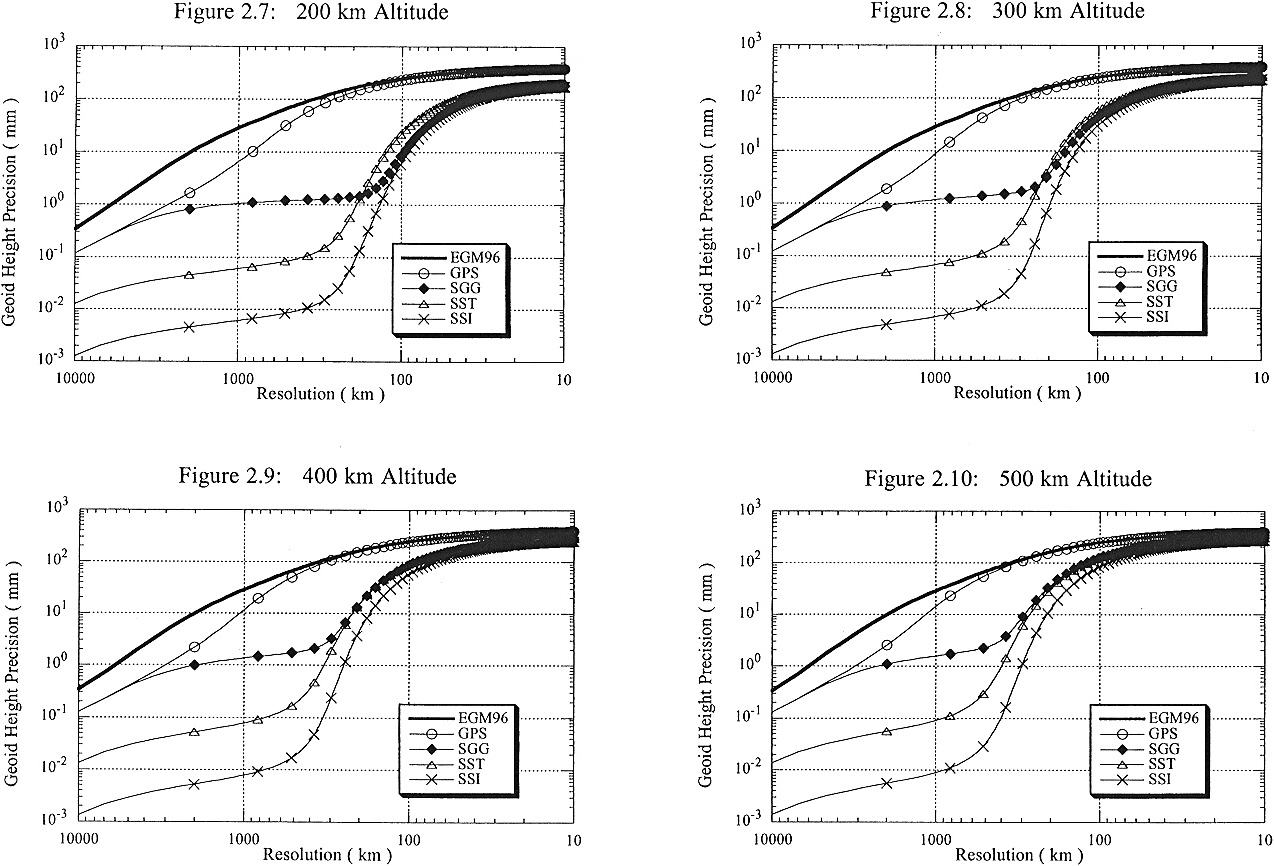
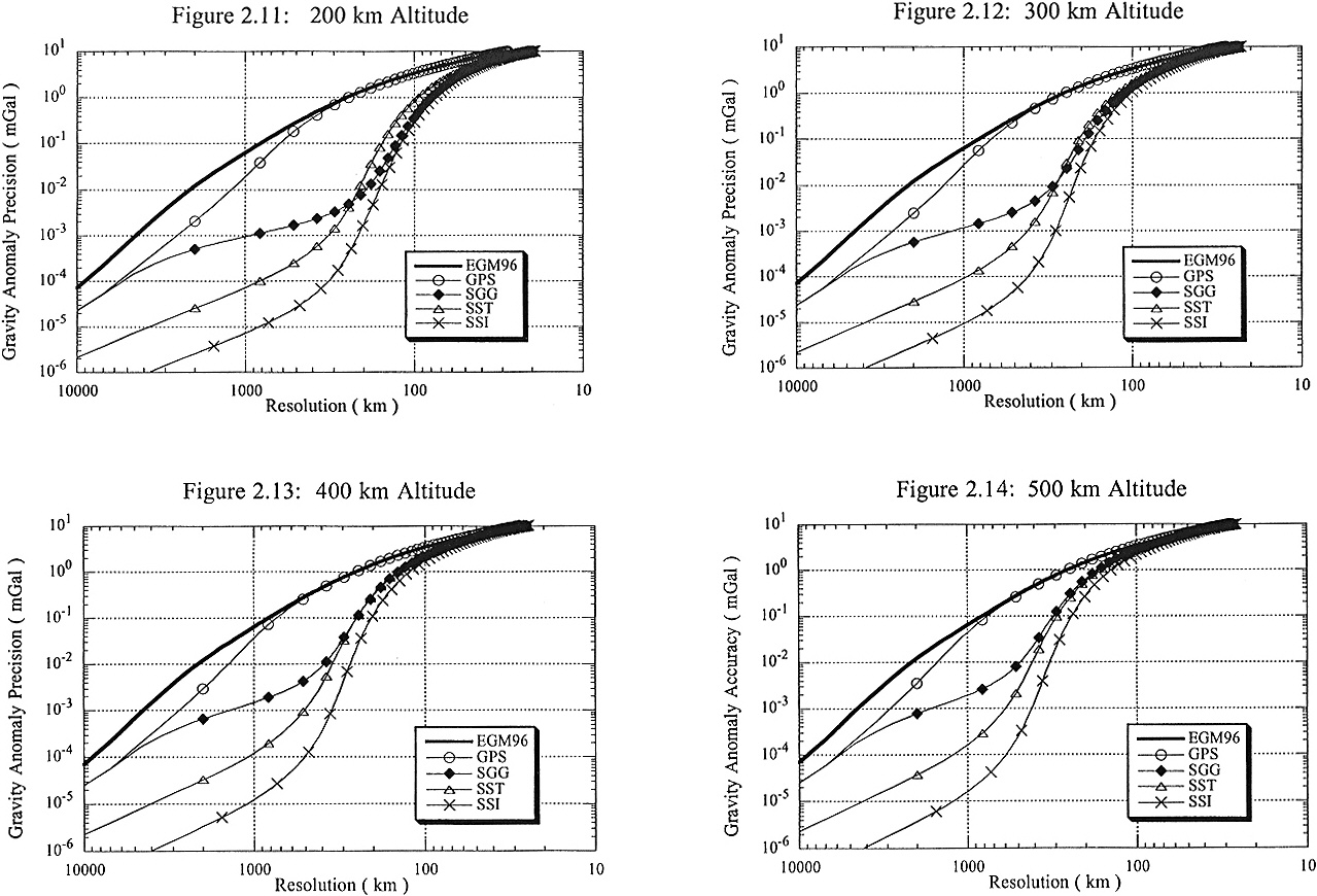
These upward trends occur where the satellite mission ceases to provide new information about the gravity field and the a priori constraint on the error takes over. Similar trends can be seen in the illustrations of gravity-anomaly precision versus resolution in Figures 2.11-2.14.
The error and resolution estimates obtained in this section are not meant to be a definitive representation of the errors realizable from actual missions. In addition to the idealizations and approximations mentioned above, there are other reasons why actual missions would be different. However, in spite of the approximations in our error-estimation technique, we feel that the gravity errors presented here are close enough to the results of more rigorous error analyses that they adequately reflect the character of the errors expected from each of the four generic missions. In particular, the variations of the errors with increasing altitude and decreasing spatial resolution should be quite accurate.
Although we have not simulated the error effects of non-gravitational or rotational influences, we do not think these will bias our results as SST and SSI missions are expected to be flown with high-precision accelerometers onboard, and the SGG missions are expected to reject these influences with careful common-mode rejection and precise alignment of the accelerometers. In addition, rigorous numerical simulations reported by Bettadpur and Tapley (1996a) indicate that, for the SST and SSI missions, the aliasing effects of low-frequency (82 cycles/revolution) accelerometer and measurement errors are greatly reduced by adjusting appropriate bias parameters simultaneously with the gravity model parameters.
Time-dependent signals in the Earth's gravity field introduce additional complications. Our simulations have assumed that the gravity field signal is constant over a 90-day period. Inspection of Figure 1.2 shows that there will be variations over this time period. The secular post-glacial rebound signal would show a change of 10-10 of gravity over 90 days with a mostly known spatial pattern. Mid-latitude cyclonic circulations in the atmosphere could generate signals of 10-9 of gravity if they varied significantly over 90 days, but these signals would also be manifest in atmospheric pressure and could be removed. Signals from very large earthquakes would also approach 10-9 of gravity, but would be at wavelengths too short for these missions to resolve. These issues are discussed further in the following chapters. The key to isolating these signals is that many of them have known spatial patterns (post-glacial rebound) or can be correlated with other observations (atmospheric pressure). Since a mixture of secular, seasonal, and interannual signals is expected, longer missions will be better able to separate these than shorter missions.
STANDARD GENERIC MISSIONS
In this chapter we have shown the effects of varying orbital altitude by modeling errors at 200, 300, 400, and 500 km altitudes. In the following chapters we will show resolution diagrams that, for clarity, use only one altitude. We have adopted 400 km as a ''standard" altitude for all missions except the SGG mission, which we show at 300 km. This is because we expect the SGG mission lifetime to be limited to 9 months by the helium dewar technology, and therefore we expect the SGG to fly at the lowest possible altitude that will allow the mission to last 9 months without carrying and burning fuel. The other missions are expected to carry fuel to re-boost their orbits; we therefore suppose that they can fly at an average altitude of 400 km for as long as 5 years. It is possible that these other missions could begin or end in a lower (300-km) orbit to increase their resolution of the static field. Our standard mission designs are summarized in Table 2.1. Note that the technologies for the SGG and SST missions are mature and ready for implementation.
In the following chapters, resolution diagrams will use the standard designs and the 90-day error estimates if the discussion is independent of time, or 5 years of independent 90-day estimates if the discussion is of time-varying constituents of the gravity field. Further details of modeling time-dependent resolutions are given in Appendix B.
CONCLUSIONS
-
There are tradeoffs between mission lifetime, altitude, and resolution. Long missions are higher and have lower resolution than short missions. Also, tradeoffs exist between temporal and spatial sampling. For example, a mission at a height of 160-170 km, which would be best for 60-km resolution (l = 350), would be a costly mission of short duration. A mission at an altitude of 400 km with a resolution capability such as we have modeled would be able to achieve its optimal spatial resolution with an orbit repeat period on the order of 40 days.
TABLE 2.1 Summary of Generic Missions
|
Mission |
Primary Measurement |
Ancillary Equipment |
Altitude (km) |
Duration (years) |
Readiness |
|
GPS |
high-low tracking by double-differenced phase |
accelerometer |
400 |
5 |
current |
|
SST |
low-low microwave tracking |
accelerometer |
400 |
5 |
mature |
|
SGG |
cryogenic gradiometer |
GPS receiver |
300 |
0.75 |
mature |
|
SSI |
low-low laser tracking |
accelerometer |
400 |
5 |
future? |
|
SGGE |
gradiometer |
GPS receiver |
400 |
5 |
future? |
-
The contributions of GPS tracking of a low satellite lie at long wavelengths. Such a mission flown at an altitude of 400-500 km would yield significant improvements over the current EGM96 results at harmonic degrees less than 25, whereas a mission flown at 300 km would contribute significant improvements at degrees up to 30.
-
The strength of the SGG mission is its high resolution, with significant improvement over the EGM96 results for degrees up to 155 at a height of 400 km and up to 215 at a height of 300 km. The short lifetime (less than one year) would limit the study of temporal variability.
-
A strength of the SST mission (the low-low mission with microwave tracking) is its high precision at long and intermediate wavelengths, hence better geoid height and gravity anomaly precisions than the SGG mission (Figures 2.7-2.10). Also, the mission lifetime (estimated to be 5 years) permits the determination of a greater range of time-varying effects.
-
The anticipated results from the SSI mission (the low-low mission with laser interferometry) are the best of the four scenarios studied. They are an order of magnitude better than the SST results at all wavelengths considered and 2 orders of magnitude better than the SGG results at long wavelengths. Technological development is required for SSI, however, whereas the technology needed for SGG and SST is mature.
-
Precision tracking by GPS is needed on all missions.


