
4—
Harvest Strategies
In addition to estimates of stock size, fisheries stock assessments also provide decision-makers with a quantitative evaluation of the consequences of alternative actions. Although the data and assessments discussed in Chapters 2 and 3 provide an estimate of the population size, recruitment rates, and other important values, the assessment process does not stop there. A biological representation of the stock dynamics must be incorporated in an evaluation of the consequences of alternative actions, encompassing the harvest strategy. The utility of assessment methods cannot be evaluated without considering how the assessments are used to choose among alternative harvest strategies.
Three related terms must be distinguished:
- Harvest strategies are the plans for adjusting management options in relation to the status of the fish stock. The two most common harvest strategies are (a) fixed exploitation rate, in which an attempt is made to take a constant fraction of the fish stock each year, and (b) constant escapement, in which an attempt is made to maintain the spawning stock size near some constant level (Figure 4.1). Management of fish populations to sustain catches and abundance levels can be based on several alternative means of strategic catch regulation. Fixed exploitation rate strategies are commonly employed in marine fish stocks under such names as FMSY, F0.1, Fmax, and F40% (defined later in this chapter). Constant escapement strategies are less commonly used, primarily for many stocks of Pacific salmon.
- Harvest tactics are the regulatory tools (e.g., quotas, seasons, gear restrictions) used to implement a harvest strategy. Harvest tactics are quite diverse, and almost all fisheries employ gear restrictions, area restrictions, and some limitation of seasons. Quotas are increasingly employed in large-scale commercial fisheries, whereas closed seasons and closed areas are common in recreational fisheries.
- Management procedures represent the combination of data collection, assessment procedure, harvest strategy, and harvest tactics.
The majority of this chapter discusses how to evaluate alternative harvest strategies, although in principle it would be considerably better to evaluate the entire management procedure.
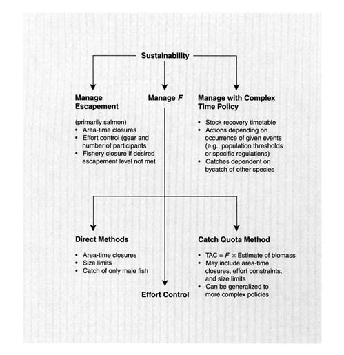
FIGURE 4.1 Role of stock assessment methods in sustainable fisheries.
Indicators of Performance
Evaluating alternative harvest strategies requires the definition of a suite of indicators to measure the expected performance of an entire fishery system including, for example, projections of fish stock size, the probability of dropping below certain thresholds, and projected catch per unit effort (CPUE). Empirical indices measure the historical performance of a fishery up to the present; analytical indices are used to project the future consequences of management decisions. In either case, the time frame of interest is typically short—about 10 years before and after the present, with greatest emphasis on present values. In Our Living Oceans (NMFS, 1996), for example, recent average yield includes only the most recent three-year period. The objectives of fishery management are seldom clearly articulated, but by noting which performance indicators are most often reported, the quantities with the greatest importance can be identified. The most common indicators involve estimates of the health of fish populations (biological indicators), the performance of the fishery (yield and social indicators), and indicators of how the uncertainty in key population parameters is likely to change in the future depending on current management actions (uncertainty indicators).
Biological Indicators
Biological indicators measure the status of a fish stock. The most widely reported indicators are trends in survey indices and trends in CPUE. For stocks that are managed using age-structured assessments, spawning stock biomass (SSB, the weight of reproductively mature fish) is an important indicator of reproductive capacity. The overfishing definitions for Atlantic mackerel, Gulf of Mexico shrimp, and northern anchovy are all based on maintaining minimum levels of SSB (Rosenberg et al., 1994). Likewise, the overfishing definitions for Pacific salmon are based on target numbers of spawning salmon. For some species, such as striped bass, a juvenile index is used to indicate the supply of recruits to the harvestable population (NMFS, 1996). Under satisfactory sampling conditions, juvenile indices can provide an effective measure of recruits (de Lafontaine et al., 1991), but problems with time-varying catchability hamper the usefulness of juvenile indices in other fishery assessments (e.g., Pacific halibut, see Quinn, 1985). The risks associated with low stock sizes include reduced fisheries landings, recruitment overfishing,* lack of forage fish for predators, and potentially irreversible changes to the ecosystem structure and function.
Yield and Social Indicators
Yield indicators measure the outputs of a fishery, namely, the recreational and commercial landings. Probably the most important yield indicator is the landed catch (landings) averaged over some time period. If the time frame of averaging is long enough to span several generations of the fish, landings also reflect the stock's SSB. Averaging is necessary to smooth out fluctuations in yield that result from environmentally driven variations in recruitment. In most stochastic models of fish populations, there is a trade-off between maximizing mean catch and minimizing the standard deviation of catch (e.g., Figure 9 in Collie and Spencer, 1993). A linear combination of yield (Y) and standard deviation of yield (SD) was used as an objective function by Quinn et al. (1990):
max[(1 - p)Y - pSD]
(4.1)
where p is a penalty weighting factor that represents the cost of one unit of increase in standard deviation in relation to one unit of increase in average yield.
Projected landings are often discounted to reflect the fact that present landings have a greater economic value than fish caught some time in the future. The present value of landings (PV) caught t years in the future is compared to the landings caught at the present time (C):
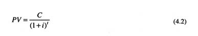
where (1+i)t is the discount factor (Clark, 1985). Although the appropriate value of the interest rate (i) is open to discussion, a relatively low discount rate of 2 to 5% is often used in fishery management studies (Walters, 1986). The choice of discount rate is important because it implicitly sets the planning horizon. The U.S. Office of Management and Budget (OMB) requires use of a 7% discount rate in the cost-benefit analyses that accompany fishery management plans.† If i = 7%, then by t = 68 years, PV will drop to approximately 1% of present landings and landings beyond 68 years have almost no present value.
|
* |
Recruitment overfishing results from fishing at a high enough level to reduce the biomass of reproductively mature fish (spawning biomass) to a level at which future recruitment is impacted. |
|
† |
OMB Circular A-94 at http://www.whitehouse.gov/WH/EOP/OMB/html/circulars, June 25, 1997. |
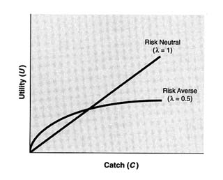
FIGURE 4.2 Fisheries utility functions.
Variability in annual landings is generally considered undesirable compared to maintaining the average yield at a constant level because variable landings create uncertainty in fishing communities and lead to the inefficient and intermittent use of capital by fishers. In fisheries with threshold harvest policies, an important yield indicator is the number of years in which the stock falls below the threshold, closing the fishery (Hall et al., 1988; Quinn et al., 1990). This penalty against allowing the stock to drop too low can be expressed more generally with the risk-averse utility function, U = Cλ (Figure 4.2), where 0 { λ { 1 (Mendelsson, 1982). With this type of concave utility function, the penalty associated with landings dropping below their mean value outweighs the benefits associated with a similar increase in landing above the mean value. A special case of the risk-averse utility function, U = log(C), has been used in studies of harvest policy (Walters and Ludwig, 1987), but it has the disadvantage of being undefined if the fishery is closed (C = 0).
The risk-averse utility function was originally formulated to describe the situation in which price is assumed to decrease as the quantity of landings increases (Clark, 1985). In this case, the benefits of increased landings above the mean level are offset by the associated decrease in price. Data on fish prices are widely available, and demand models exist that can be used to project prices as a function of harvest. The landed value (landed weight of fish in kilograms times price per kilogram) is a common performance indicator that represents the gross benefits from a fishery. Ideally, the net benefits can be calculated by subtracting the costs of catching the fish, managing the fishery, and other related activities. In practice, fishing costs are difficult to measure and net benefits can seldom be estimated reliably. In some fisheries with a risk-averse utility function, when price per unit declines as landings increase, any decrease in TAC to help increase price per unit is lost if the landings are made up through imports. This actually exacerbates, rather than relieves, the economic problems for fishers. Some yield indicators can also function as social indicators, such as net economic benefit from a fishery. Other social indicators are employment in the fishery and associated industries and average debt burden of individual fishers and fishing companies.
Uncertainty Indicators
A final class of performance indicators measures the rate at which analysts can learn about uncertain population parameters. Some harvest policies may be more informative than others in reducing parameter uncertainty or allowing the analyst to choose among a set of competing hypotheses about stock production (Walters, 1986). It follows that a more informative harvest policy should lead to better management and increased future benefits. Four measures of learning performance were discussed in detail by Walters (1986). In brief, high performance is
associated with minimizing the uncertainty about key population parameters and policy variables and minimizing the error in predicting future stock sizes.
Biological Reference Points
The 1992 guidelines for fishery management plans (50 CFR, Part 602) stipulate that overfishing definitions must exist for all stocks managed under federal fishery management plans. For this reason, much effort has been devoted to defining overfishing thresholds (Rosenberg et al., 1994). Biological reference points (BRPs) are calculable quantities that describe a population's state. They can be used as targets for optimal fishing, as well as for setting overfishing thresholds. They are calculated from the life-history characteristics of a given stock and are used to define harvest control laws (Figure 4.3). A BRP can be expressed as a fishing mortality rate (F) and/or as a level of stock biomass (B). BRPs can be targets or thresholds.
A threshold control rule specifies the upper limit of fishing mortality allowable or the lower biomass limit beyond which overfishing occurs. A target control rule is more conservative than a threshold and defines a desired rate of fishing and acceptable levels of stock biomass. It is wise to have some separation between the target and threshold levels, so that minor overruns of targets will not exceed the thresholds. For many depleted stocks, the overfishing thresholds have become de facto targets, contrary to the intent of the overfishing definitions, leaving no buffer to accommodate occasional overestimates or unexpected negative environmental factors. For example, pollution events, disease or predator outbreaks, and unusually warm or cold water temperatures can affect fish stocks unexpectedly. More complicated strategies involving yield per recruit (e.g., eumetric fishing [Beverton and Holt, 1993]) have been considered but have been superseded for the most part by direct consideration or more detailed modeling of selectivity and catchability. Annex II of the Agreement for the Implementation of the United Nations Convention on the Law of the Sea of 10 December 1982 Relating to the Conservation and Management of Straddling Fish Stocks and Highly Migratory Fish Stocks (which the United States has ratified) provides guidelines for applying precautionary reference points for managing populations of highly migratory fish species and those that straddle national boundaries (UN, 1995).
Fishing Mortality Reference Points
The natural mortality rate (M), or some fraction of M, has been used in some fisheries to set the F value that would constitute overfishing (e.g., for North Pacific groundfish). The rationale for this approach is that short-lived species with high M (and presumably a high intrinsic rate of increase) should be able to sustain a higher F level

FIGURE 4.3 Schematic harvest control laws.
SOURCE: Modified from Rosenberg et al. (1994).
NOTE: mt = metric tons.
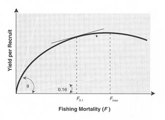
FIGURE 4.4 Method of defining F0.1, given a known relationship between fishing mortality rate and yield per recruit, as the point on the Y/R curve at which the slope of a line tangential to the curve is one-tenth the slope of a line tangential to the curve at the origin.
than long-lived species with low M. Indeed, many fish stocks that have sustained fisheries for long periods have sustained fishing mortality rates near M (Mace, 1994). Unfortunately, M is not well known for most fish stocks, and estimated values must be used in stock assessments. Two common M-based reference points use the yield per recruit (YPR) or spawning biomass per recruit (SPR).
Yield per Recruit
YPR is the total yield in weight harvested from a year-class of fish over its lifetime, divided by the number of fish recruited into the stock (Figure 4.4). The relationship between YPR and F is useful for defining several BRPs. The threshold level Fmax is the fishing mortality that maximizes PR. Levels of fishing mortality higher than this reference point constitute growth overfishing because individuals are harvested before they have grown to a size that will maximize YPR. Fmax is used as an overfishing definition for summer flounder and scup in the northeastern United States. It is possible to calculate the age of first entry to the fishery (or mesh size) that will result in a given YPR with a minimum expenditure of fishing effort.
Another reference level (F0.1) is defined as the F at which the slope of a line tangential to the YPR curve is one-tenth of its slope at the origin (Gulland and Boerma, 1973; Figure 4.4). Despite its arbitrary definition, F0.1 is desirable because it is a target reference point that is lower than Fmax and therefore provides a buffer to avoid growth overfishing. The F0.1 level increases yield per unit effort without sacrificing much yield and has been widely used as a target F (Deriso, 1987). F0.1 also has some basis in bioeconomics because it is the point at which each additional unit of fishing mortality achieves less than 10% of the yield per recruit obtainable from a unit of fishing mortality applied to a previously unexploited stock; that is, the return (in units of catch biomass per recruit) on investment in a unit of fishing mortality is 10% of the return obtainable from the stock when it was in an unexploited condition. The product of equilibrium recruitment (R) and YPR can be used to define FMSY, the fishing mortality for maximum sustainable yield (MSY; Figure 4.5).
Spawning Biomass per Recruit
A common SPR-based reference level, FX%, is defined as the F that would reduce the spawning stock biomass per recruit to X% of the level that would exist with no fishing. Many of the overfishing definitions for U.S. fish stocks are based on an FX% (Rosenberg et al., 1994) because it relates directly to SSB, the quantity to be conserved. Specifying the FX% to use as a reference level is somewhat arbitrary; recent work has sought to define FX% values that are analogous to F0.1. For example, Clark (1993) and Mace and Sissenwine (1993) suggest that levels of F35% to F45% are appropriate, as explained below. Spawning biomass per recruit is complicated in
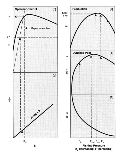
FIGURE 4.5 Single species theory of fishing. A dynamic pool model (a and d) describes the effect of fishing mortality rate (F) and age at capture (tc) on spawning biomass (S) per recruit (R) and yield (Y) per recruit. A spawner-recruit model (c) relates the number of recruits to spawning biomass; a ''replacement line" with slope equal to the inverse of S/R is mapped by a graphic procedure (b). S and R must be scaled to appropriate units (e.g., thousands of tons and millions of fish, respectively) for the graphic procedure to be practical. The intersection of the replacement line with the spawner-recruit function determines equilibrium recruitment. The product of equilibrium recruitment (c) and yield per recruit (d) is the equilibrium production (e). The method is demonstrated for a fishing mortality rate of Fro (conditional on an unspecified value of tc). FMSY is indicated based on the production model (c); F0.1 and Fmax are indicated in (d).
SOURCE: Sissenwine and Shepherd (1987).
Used with permission from Canada's National Research Council Press.
TABLE 4.1 Relationships Between Fishing Mortality Reference Levels and Spawning Biomass Per Recruit
|
BRP |
Corresponding Average %SPR |
Reference type |
|
F0.1 |
38 |
Target |
|
Fmax |
21 |
Threshold |
|
Fmed |
19 |
Threshold |
hermaphroditic fish, which comprise a minority of commercial species, primarily reef dwellers in tropical and semitropical regions.
Shepherd (1982) first showed how SPR analysis could be combined with stock-recruitment (S-R) observations* to generate reference fishing mortality rates. An example is Fmed, the fishing mortality rate that results in an SPR equal to the inverse of the median survival ratio (number of recruits produced per unit of spawning biomass [R/SSB]). Sissenwine and Shepherd (1987) suggested Fmed as an overfishing threshold because a stock harvested at this rate (or lower) should be able to replace itself on average, but Fmed is based on observed survival ratios, which depend on the exploitation history of the stock. If Fmed is estimated after a stock has been exploited heavily, its value will be too high and the stock will be depleted. Conversely, Fmed may be a very conservative threshold in the case of stocks that are exploited only lightly before it is determined.
Several studies have examined the BRPs among stocks, and the mathematical relationships among BRPs, to determine the most appropriate target and threshold levels (Deriso, 1987). For 91 well-studied stocks, Mace and Sissenwine (1993) computed the %SPR corresponding to fishing mortality reference levels (Table 4.1).
Clark (1991) examined a range of life-history parameters typical of demersal fish to determine the level of fishing mortality that maximizes the minimum yield (Fmmy) over a range of typical S-R relationships (Fmmy is the best fishing mortality rate for minimizing lost harvest). Clark found that in general, Fmmy![]() F35%
F35%![]() F0.1 and advocated F35% as a target F, except for stocks where recruitment and maturity schedules do not coincide. Subsequent trials indicated that a slightly higher %SPR of about 40% is desirable in the presence of high serial correlation in recruitment from year to year (Clark, 1993).
F0.1 and advocated F35% as a target F, except for stocks where recruitment and maturity schedules do not coincide. Subsequent trials indicated that a slightly higher %SPR of about 40% is desirable in the presence of high serial correlation in recruitment from year to year (Clark, 1993).
Many species appear to have strongly compensatory S-R relationships; that is, per capita recruitment increases significantly as stock size decreases. Reference levels are now more commonly based on a %SPR, but the percentage is often specified by analogy with other stocks or by using the results mentioned above. A knowledge of the compensatory capacity of the stock is necessary to define the most appropriate BRPs for a stock. Even without such knowledge, however, a conservative %SPR still can be selected (Sissenwine and Shepherd, 1987).
Biomass-Based Reference Points
Biomass-based reference points may be defined as sharp thresholds or as sliding scales to reduce fishing mortality as stock size declines progressively. Observed stock-recruitment data can be used to define biomass thresholds. Biomass thresholds can also be defined from fitted S-R relationships. An example is the SSB corresponding to 50 percent of the maximum expected recruitment (Mace, 1994). These estimators are easily understood and relatively robust if only data at low stock sizes are available and almost always result in higher levels of recruitment above the minimum biomass threshold (Myers et al., 1994).
A biomass threshold can be defined as a percentage of the estimated unexploited stock size (B0), for example, 20%B0 (Beddington and Cooke, 1983; Quinn et al., 1990). The appropriate percentile depends on the compensatory capacity of the stock; stocks with higher compensatory capacity can sustain a lower biomass threshold. B0 must be estimated either with a stock-production relationship or by assuming that the earliest recorded biomass represented an unfished condition. Finally, stock-production relationships can be used to estimate BMSY, which
may be considered a target biomass level, the biomass at which maximum sustainable yield could be attained. As mentioned earlier, Atlantic mackerel, Gulf of Mexico shrimp, and northern anchovy stocks are managed using biomass-based BRPs. The North Pacific Fishery Management Council recently established a default threshold of 5% of unfished biomass and a biomass-based adjustment to decrease F at low population sizes. Many Alaska salmon populations have target minimum biomass levels (in numbers of fish).
The most appropriate reference point chosen to manage harvest from a specific stock depends on how environmental variability affects the dynamics of the population. Environmental variability can affect population growth rates directly via density-independent rate processes (Beddington and May, 1977) or via density-dependent processes and equilibrium abundances (Roughgarden, 1975; Shepherd and Horwood, 1979). The latter case is consistent with variability at long time scales (Pimm, 1984) as is the case for marine fishes. Consider the Ricker model:
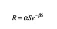
If environmental variability affects the density-independent parameter (α), a minimum biomass threshold may be required in addition to an F-based BRP. If environmental variability affects the density-dependent parameter (β), a biomass threshold may not be necessary. The effects of environmental variability make a difference in the way the population will respond to harvesting.
The advantages and disadvantages of fishing mortality rate and biomass-based reference points were discussed at length by the panel that examined the definitions of overfishing in U.S. fishery management plans (Rosenberg et al., 1994). Fishing mortality reference points are generally easier to calculate and more robust than biomass reference points when limited data are available. Biomass thresholds are needed, particularly for stock rebuilding, but there are still no widely accepted methods available for deriving biomass thresholds. Biomass thresholds can increase the average yield, with a corresponding increase in the variability of yield. Rosenberg et al. (1994) recommended that control laws combine a maximum fishing mortality rate and a precautionary biomass level wherever possible.
Closed-Loop Management Strategies
Harvest strategies based on fishing mortality rate or biomass targets modify harvest tactics depending on the stock assessment results and thus are "closed-loop" strategies in the terminology of control systems theory. In this closed loop, there are tight linkages: regulatory performance depends on assessment performance and assessment performance in turn depends on the regulatory pattern. Sustaining fish populations requires management procedures and practices that can cope with considerable uncertainty about population dynamics and the accuracy of stock assessments.
Input Control
Input controls limit inputs such as effort (labor) and capital that can be devoted to a fishery. Early research on management under uncertainty focused primarily on designing policies for dealing with unpredictable variation in recruitment and survival rates. Most of this research did not consider errors in assessments of stock size. A basic finding during the mid-1970s and later (Reed, 1974; Clark, 1985; Mangel, 1985; Hilborn and Walters, 1992) was that the optimum management in the presence of recruitment variation involves following a "feedback strategy" rule that specifies the best fishing rate and/or quota to select each year as a function of the stock size that year. The notion of harvest strategies has since become associated with such rules, in applications ranging from whales to salmon management to current National Marine Fisheries Service (NMFS) rules for varying fishing mortality rate with stock size.
Optimal rules were found generally to be simple, involving either (1) trying to maintain a fixed escapement*
or base stock (rule: harvest annual excess of biomass over base) or (2) trying to maintain a fixed exploitation rate (rule: harvest same proportion of biomass each year). The shift from input control to output control (see below) resulted from the realization that determining the correct F or harvest is only part of the management problem. Implementing the proper F is also difficult. Implementation of output controls was motivated by a desire to implement F control as efficiently as possible, in an economic sense.
Output Control
During the late 1970s, considerable research was conducted by economists regarding how to improve the economic performance of fisheries, and this work led to the idea of "output control" via individual fishing quotas.* It was noted that ownership of predictable shares of allowable harvest can lead to much more efficient harvest planning and participation in management than occur in historical input control situations in which limits on effort or total quota lead to intense competition among fishermen for available fishing opportunities. Output and quota management policies have become increasingly popular with fishery managers, both because they are presumed to lead to better economic performance and because such policies simplify the manager's responsibilities. Under individual quota management, issues of catch allocation among stakeholders can be resolved by trading among stakeholders of their clearly denominated shares of the catch, with little intervention from managers. Responsibility for determining how large the total allowable catch (TAC) should be, given stock assessments and uncertainties, is often assigned by the manager to scientific assessment teams and processes.
There have been a few recent attempts to evaluate whether constant quota policies (rule: take the same quota each year independent of stock size variations) might still be economically optimum even if the quota were adjusted downward to allow for natural variation in recruitment (Hannesson, 1989; Arnason, 1993). The general result of these evaluations has been to recommend that quotas should not be held constant because in most cases a safe constant quota level would be too low compared to the long-term average MSY that could be obtained under a regime of variable annual catches. This has led to the recommendation that annual quota should vary with stock size and that quota shares should be set as proportions of the annual TAC.
Implementation Problems with Constant Exploitation Rate Strategies
Even where quota management has not proceeded to the individual fishing quota approach recommended by many economists, there has been wide acceptance of the simple strategy rule TAC = F × EB, where F is the target fishing mortality rate (e.g., Fmax, F0.1, FX%) and BE is the exploitable biomass. Constant exploitation rate or constant-F strategies are in principle very simple and have been shown to be nearly optimal in cases where the primary management objective is risk averse (Deriso, 1985) and in situations where long-term changes in the carrying capacity of marine ecosystems cannot be anticipated significantly in advance (Walters and Parma, 1996). These policies are robust to underestimation of the optimum F; using an F value lower than optimal for a given stock, although it will result in lower catches, can actually lead to higher biomass than optimum, and this increase in biomass partially balances the effect of using a lower-than-optimum F because the spawning stock is overprotected and gains will be achieved in later years. A variation on constant-F policies is to set a lower biomass limit, below which the target F is reduced to promote more rapid stock rebuilding (e.g., Quinn et al., 1990). With a depensatory stock-production relationship,† the optimal harvest strategy is to vary F in relation to stock size (Spencer, 1997).
Early research on performance of constant-F strategies presumed either that stock size is estimated accurately
or that F can be regulated directly by regulating fishing effort. Indeed, TACs and effort control were the two most commonly used tactics for implementing constant fishing mortalities. It was assumed in early assessment methods that F = q × Effort, with the catchability q representing a constant proportion of stock caught by one unit of effort. Variation in q over time was expected because of changes in fishing technology; therefore, many methods were developed for standardizing effort to some constant q value. However, a number of recent stock collapses, along with analyses of the behavior of fishers and fish, have indicated it is highly likely that q increases rapidly as stock size declines. That is, fixing effort is no guarantee of a safe F value; F can increase substantially as stock size declines if the geographic range used by the fish shrinks and fishers are able to track this contraction so as to target remaining fish concentrations efficiently, thereby increasing q. Such a situation has occurred, for example, with the Peruvian anchoveta.
Conversely, setting the TAC equal to the target F multiplied by an estimate of biomass is controversial because it has placed a significant responsibility on stock assessment to provide good estimates of biomass (or at least estimates that are not often greater than actual biomass). Simulation tests of long-term management in which TAC is set as a constant fraction of an uncertain biomass estimate indicate that biomass estimation errors with coefficients of variation (CV) greater than 50% are likely to result in substantial degradation in long-term harvest performance, particularly for highly productive stocks (Eggers, 1993; Frederick and Peterman, 1995; Walters and Parma, 1996). Following an approach similar to that described in Walters and Parma (1996), the committee simulated long-term performance of constant-F policies for two prototypical cases, referred to as "herring" (a short-lived, rather productive stock with optimal harvest rate equal to 0.25) and "cod" (a long-lived, less productive stock with optimal harvest rate equal to 0.10). The simulations were conducted by assuming that errors in the annual estimates of biomass were lognormally distributed and that population carrying capacity changed randomly from year to year with correlation r = 0.3 or 0.8 between total catch and the CV of biomass estimates (Figure 4.6). Three different harvest strategies were simulated: optimal escapement, optimal F, and risk-adjusted F.
Simulation results presented in Figure 4.6 indicate that degradation is more severe when estimation errors are strongly autocorrelated, for example, as expected when the estimates are based on fitting times series of data to population dynamic models. As expected, an increase in the CV of estimated biomass resulted in a lower catch for all harvest strategies and both levels of autocorrelation. However, the risk-adjusted F harvest strategy seemed to be less affected by increasing CVs. In addition, with autocorrelation, the probability that the stock falls to low, potentially dangerous levels may increase because successive errors no longer cancel out as they do to some extent when estimation errors are independent from year to year. This degradation could become critical in situations in which biomass estimates tend to be greater than actual biomass levels during stock declines. Such a situation typically occurs when catch-at-age analysis is tuned with CPUE data and CPUE does not decrease in proportion to abundance because fishers are targeting constricting stocks (this is illustrated by data sets 1-4 in the committee's simulations (see Chapter 5).
Faced with the possibility that inaccurate stock assessments will cause TAC (and hence F) to be set too high, the fishery manager has three strategic options:
- ignore the danger and accept the degradation in long-term fishery performance resulting from the F variation (this degradation can be as much as 50% of potential fishery value [Walters and Parma, 1996]);
- use a risk-adjusted biomass assessment in the TAC = F × EB calculation; or
- use a risk-adjusted F assessment in the TAC calculation.
Simulation studies (Frederick and Peterman, 1995; Walters and Pearse, 1996) indicate that risk adjustment factors (i.e., the factor by which F is reduced to account for errors in the estimate of EB) may be substantial, approaching or exceeding exp {-0.5 CV2}. In practice, risk adjustment factors do not have to be calculated, provided the harvesting strategies are evaluated by assuming realistic errors in the estimation of stock size. In the simulations shown in Figure 4.6, biomass estimates had a log normal error with a median of zero and bias equal to exp{0.5 CV2}, so a risk adjustment equal to exp{-0.5 CV2} was used. The degradation in average performance of risk-adjusted F policies with increasing CV was much less severe than when an optimal equilibrium F policy was assumed. Yield losses could still be substantial for CV } 0.5 in some trials, especially when estimation errors were
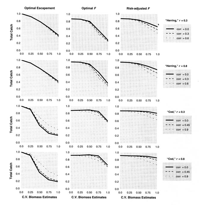
FIGURE 4.6 Effect of stochastic errors in annual biomass estimation on performance of escapement and fixed exploitation rate strategies. Average 100-year catches are expressed as a fraction of the maximum total yield achieved when all future recruitment deviations are known in advance and stock size is known without error. Optimal escapements are computed by using dynamic programming and assuming no estimation errors; optimal F corresponds to the fixed exploitation strategy that maximizes long-term average catches; risk-adjusted F = optimal F exp{-0.5 CV2}, where CV is the coefficient of variation of biomass estimates. Three levels of autocorrelation in the estimation errors (corr) were used, with the maximum set equal to the growth-survival parameter of the delay-difference model used in the simulations (see Walters and Parma, 1996, for further details). Carrying capacity was assumed to fluctuate as an autoregressive random process with correlation given by r. Each plot is the average over 100 random series of environmental trends and 100 biomass estimation trials done on each of them.
assumed to be serially correlated. The probability that the stock biomass fell below 20% of average during the first 20 years of simulation (Figure 4.7) could still be high even under the risk-adjusted harvest rate, especially for very productive stocks (the "herring" case).
In summary, the two most common tactics for implementing fixed harvest rate policies—effort control and quota control—imply that managers must either obtain accurate biomass estimates to set TACs or use input regulation of fishing effort. Either approach entails the risk that F will increase dangerously with accidental decreases in stock size. This apparent dichotomy does not in fact cover all options for achieving constant F (Walters and Parma, 1996; Walters and Pearse, 1996). There are a variety of other tactics for preventing high F besides effort regulation, such as large marine refuges and direct assessment of cumulative F using tagging during a given season. Complementing quota management with space and/or time harvesting restrictions that directly limit the proportion of fish exposed to harvest may prove a costly but effective way of placing a firm upper bound on F.
When evaluating such regulatory schemes, the costs of placing a large number of fishers in competition in a substantially reduced time period and geographic area must be weighed against the costs of following more standard harvest tactics under realistic assessments of risks. The results of simulation experiments such as those cited above are particularly worrisome because they indicate that yield losses due to biomass estimation error in systems where TACt = F![]() t can exceed the gains in economic performance expected from individual quota management (from reduced competition and more efficient deployment of fishing activity). In short, it does not make much sense to move to a quota management system if the quota must be corrected downward so far as to wipe out the gains from having it in the first place. Alternative regulatory approaches involving direct control of harvesting risks through area-time closures must be considered experimental at this time.
t can exceed the gains in economic performance expected from individual quota management (from reduced competition and more efficient deployment of fishing activity). In short, it does not make much sense to move to a quota management system if the quota must be corrected downward so far as to wipe out the gains from having it in the first place. Alternative regulatory approaches involving direct control of harvesting risks through area-time closures must be considered experimental at this time.
Improve Management Strategies or Improve Assessments?
Application of risk-adjusted (based on F or biomass) reference points would immediately lead to reduced TAC and create an economic incentive for investment in improved data gathering and assessment procedures to reduce the CV of biomass estimates (Pearse and Walters, 1992; Walters and Pearse, 1996). The committee can offer no clear and general recommendation about where to direct this investment from among the three plausible options:
- increase sample sizes in existing data gathering programs (surveys, age composition sampling, tagging);
- initiate new sampling programs to provide auxiliary data such as relative abundance of pre-recruits, egg surveys, and direct estimates of F based on tagging; and/or
- invest in development and implementation of "better" assessment models for making more effective use of existing data.
Monte Carlo simulations of performance improvements that can be achieved by type 1 investments (e.g., Walters and Collie, 1989) suggest that only limited opportunities are available for reducing CVs of biomass estimates solely by gathering more of the usual data. In general, variability among observations in surveys and variability in age composition due to multinomial sampling appear to greatly underestimate the actual uncertainty in these key types of assessment data. That is, year-to-year and among-age variances in the measurements are substantially greater than expected from within-sample variance and sample size calculations, indicating that some major sources of variation are not accounted for in assessing the precision of these data sources. For example, survey abundance estimates often vary more from year to year than would be expected based on standard calculations of sampling variance (as in Chapter 2) and maximum variability that is biologically possible given recruitment and survival rates. Given this consideration, any assessment of the value of gathering more of the same data would be highly suspect, and would most likely be overly optimistic.
The development and use of Stock Synthesis models and related multi-data-type procedures are generally viewed as investments of types 2 and 3. There has been little exploratory work using Monte Carlo simulation to ask "what if we had data of type X?" questions related to available assessment procedures; only recently have
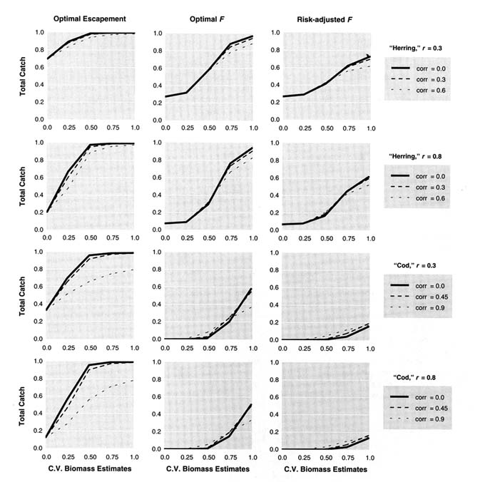
FIGURE 4.7 Effect of stochastic errors in annual biomass estimation on the probability that stock biomass falls below 20% of average carrying capacity at least once during the first 20 years of simulation. Each simulation starts with stock biomass at the optimal equilibrium size. Further details are provided in the caption for Figure 4.6.
multi-data assessment procedures such as Stock Synthesis (Methot, 1989, 1990, Bence et al., 1993) become available to allow realistic answers to such questions. It is not at all obvious that merely adding more auxiliary data and corresponding complexity in the assessment model (more "nuisance parameters," more structure) will produce more precise biomass estimates. Experience with simulation of closed-loop management performance using deliberately oversimplified assessment models has indicated that it can often be better (in terms of long-term average catch) to use a simpler assessment model that could be parameterized with available data (Hilborn, 1979; Ludwig and Walters, 1985, 1989). The basic problem here is that assessment using more complex, realistic models may provide more accurate estimates, but these estimates are likely to be less precise (have higher variance) than estimates from oversimplified models (Figure 4.8).
Basic statistical theory demonstrates the negative effects of over-parameterization in cases where a sequence of increasingly complex assessment models is fit to a fixed set of historical data. It is not yet clear, however, how performance changes when there is simultaneous addition of model complexity and more auxiliary data. Although oversimplified models may outperform more realistic ones for implementing some closed-loop decision rules, the estimates of uncertainty about key management parameters (e.g., exploitable biomass) based on oversimplified models will be too optimistic and should not be used as a basis for policy evaluation. Thus, the optimal model for policy evaluation may be more complex than the optimal model for estimating population parameters in a stock assessment.
When Closed-Loop Management Strategies Are Most Likely to Fail
The two stock assessment situations most likely to result in persistent bias in stock size estimates occur when (1) stock size is collapsing rapidly and (2) stock size is very low and there is uncertainty about whether recovery is possible.
Stock Collapse
During stock collapses, overestimation of remaining abundance will lead to excessive harvesting, in which exploitation rate may even increase as the collapse proceeds (when quotas or TACs are not being reduced as rapidly as stock size). Overestimation of stock size during collapses has occurred primarily in situations in which (1) age-structured assessment methods have incorporated fishery CPUE data that do not decrease in proportion to stock size (cod stocks in Canada and herring in the North Sea are major examples; see simulated data set 1 in Chapter 5); and/or (2) where vulnerability of younger age classes has increased over time due to growth changes or changed targeting practices by the fishery (leading in virtual population analyses to an appearance that recruitment has been higher than actual).
Recovery Situations
During recoveries, overestimation of stock size will lead to overly optimistic assessments of how soon the fishery can be reopened or how much yield will be sustained in the future (e.g., northern cod stock in Canada from 1978 to 1985). Transient upturns in the indices of abundance may lead to false expectations of recovery when the political climate is favorable to relaxation of fishing restrictions (e.g., king crab from Kodiak, Alaska, in 1981; Orensanz et al., in press). Recovery trends following severe restrictions in fishing pressure are difficult to assess because catches are small relative to surplus production. Standard assessment methods do not work well unless fishery removals are significant because catches are generally the only quantities measured in absolute units that provide the scale of biomass estimates.
Fishery-independent surveys constitute the only way to guarantee that actual abundance trends will be detected by the assessment system, although having such surveys does not guarantee that trends will be assessed correctly, as some of the results of simulations reported in Chapter 5 indicate. Many surveys have been developed without careful consideration of how the spatial structure of stocks is likely to change over time, for example, surveys that are designed to cover areas of highest abundance or convenient sampling locations, rather than the full
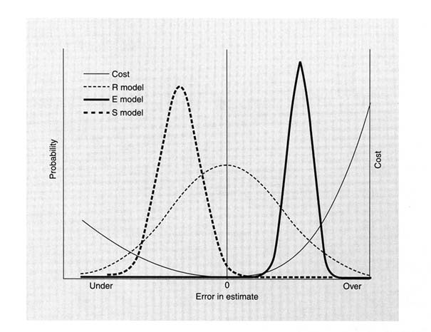
FIGURE 4.8 Uncertainty in estimates of policy parameters such as allowable catch depends on the model used for estimation. There is a cost to making estimation errors, which is generally asymmetric since overharvest tends to be more costly than underharvest. Estimates can be quite variable (R case) when realistic models are used with uninformative data, resulting in high expected costs (high odds of estimates being far enough off to produce high costs). Expected cost equals the sum of the probability of an error multiplied by the cost at each potential error level. Estimates from very simple equilibrium models (E case) fit to the same data may be quite precise but dangerously biased (i.e., the distribution is narrow but centered above zero). Given existing limitations in modeling and sampling, which often preclude estimates that are both precise and accurate, the most appropriate assessment model (S case) often is a deliberately oversimplified model that is not too badly biased (in a safe direction), and gives less variable estimates than would be achieved with a more realistic model. SOURCE: Redrawn from Walters (1996).
range of the stock. A survey with a poorly designed survey frame (too small a sampling area, near the "core" range of the stock into which abundance contracts as the stock declines) may show the same incorrect trends as commercial CPUE. For example, surveys of Pacific Ocean perch in Goose Island Gully off British Columbia did not indicate a major stock decline in conjunction with high fishery removals during the 1960s; there is a nagging fear among biologists that the stock was depleted far more severely than surveys indicated and that the survey frame was too small (did not extend far enough into deep water) to detect the full extent of the decline.
Recreational Management Strategies
Many coastal fisheries are changing rapidly from commercial to recreational status; large and effective recreational fishing lobbies have had much political influence on allocation, basing their case on the higher
economic value of each fish taken by recreational fishing than by commercial fishing and on the fact that recreational anglers represent a large voting block (these forces are identified here to emphasize that the trend is not likely to be reversed). A number of serious assessment and harvest strategy problems result from this trend (see also Chapter 2), including the following:
- loss of abundance indices and catch composition data from the commercial fishery;
- drastic increase in the cost of basic catch and effort assessment because a larger number of more disperse units must be sampled;
- large changes in the space and time distribution of fishing and associated size or age vulnerability patterns; and
- entrenchment of an open-access system in recreational fisheries without any option for simple regulatory instruments such as total quotas or total effort limitation.
Biologists have not been too concerned in the past about overfishing in recreational fisheries, believing that recreational methods are generally relatively inefficient and that any depletion of stock should result in decreasing effort and cause a feedback reduction in harvest rate. This lack of concern about modern recreational fisheries is unwise; recreational methods are becoming much more efficient, recreational fishers are becoming more numerous, and they often target a mixture of species so that a decline in particular species is no guarantee that total effort and fishing mortality risk will decrease in response. Existing regulations, bag limits, and minimum sizes in recreational fisheries are unable to constrain recreational catches to target levels. Recreational harvests can greatly exceed target catches, sometimes by as much as 100%, so that total harvests are unsustainable even when commercial catch limitations are enforced. Because recreational fisheries are such a large component of fisheries harvests for many coastal fish species, it is necessary to include recreational fisheries in risk-averse harvesting strategies.
In principle, strategies used for varying exploitation rate with stock size in commercial fisheries could also be used in recreational fisheries to meet similar objectives for long-term sustained stock sizes and the opportunity for anglers to remove as many fish from the water as possible over the long term. In situations in which the recreational value of fisheries derives mainly from the ability to attract tourists to a region, the best management strategy might place more emphasis on maintaining high abundance of larger fish (and great attractiveness of the fishery compared to other options for the angler) than on high catch. However, such strategic trade-offs are not really the most important problem in recreational fisheries assessment; a significant difficulty has been in assessing the impact of alternative options for achieving desirable harvest rate strategies. Tactics for regulation of recreational fisheries include measures such as individual bag limits, size limits, space and time closures, and catch-release requirements. Evaluation of these measures almost always requires analysis of fish biology and fisher behavior at space-time-stock structure scales far more detailed than those used in commercial stock assessment. For example, a regulatory options model for Pacific salmon was used to examine chinook and coho stocks on time scales of weeks, to keep track of size-age structure in great detail, and to provide a complex accounting procedure for processes such as release of undersize fish and associated impacts on survival and later vulnerability to fishing (Argue et al., 1983). Such detailed calculations were necessary to even approach an accurate representation of the cumulative impact of such apparently simple policies as minimum size limits.
In general, there are few data on catch and effort from recreational fisheries. However, considerable information regarding age and growth, as well as other life-history characteristics is often available. Therefore, stock assessment scientists for recreational fisheries have tended to base their recommendations on yield-per-recruit and spawning biomass-per-recruit models. Some references dealing with these approaches include yield-per-recruit models for recreational fisheries (Buxton, 1992; Quinn and Szarzi, 1993), simulation models for minimum size limits and closed seasons (Atwood and Bennett, 1990), age and growth studies (Smale and Punt, 1991), and marine reserve evaluation by Atwood and Bennett (1995).
Not only are recreational fisheries more expensive to monitor and more difficult to regulate than commercial fisheries, they also may demand far more detailed and sophisticated assessment models for evaluating alternative harvest strategies. The development of such models is in its infancy, with some examples available in the literature
(Argue et al., 1983; Quinn and Szarzi, 1993; Szarzi et al., 1995). Conversely, relatively unsophisticated assessment models have been applied with success to recreational fisheries in South Africa (e.g., Smale and Punt, 1991; Buxton, 1992) and elsewhere.
Impact of Responsible Fishing on Management Strategies and Closed-Loop Performance
The Food and Agriculture Organization adopted a global Code of Conduct for Responsible Fisheries on October 31, 1995, providing a framework for voluntary national and international efforts to exploit living aquatic resources in a sustainable manner while minimizing environmental impacts.* NMFS intends to adopt a version of this code after receiving public input. Bycatch is a major source of fish mortality (Alverson et al., 1994), and the move to responsible fishing practices may require major changes in fishing gear toward more selective methods to reduce bycatch. From a stock assessment perspective, movement to better gear types will add uncertainty about changes in age-size selectivity patterns, natural mortality, and pre-recruit mortality rates. Also, relative abundance indices based on historical fishery methods and statistics will be invalidated (this may actually be a benefit if CPUE statistics are as widely misleading as some scientists believe). For some fisheries, especially those in which assessment has been based on production modeling and relative abundance data rather than age-structured data, changing gear creates a situation similar to having no historical experience and starting assessments from scratch on a new fishery.
There are two main ways to guard against severe stock assessment problems during the transition to responsible fishing practices: (1) ensure that fishery-independent survey systems are in place for as long as possible before the transition begins, even if this means delaying the transition by a few years to gather baseline data; and (2) include regulatory measures (e.g., spatial closures) that directly limit exploitation rate during the transition period. The second of these points is particularly critical. It is often assumed that more selective and responsible fishing methods will be less efficient than the methods they replace; otherwise, the selective methods would already have been implemented for obvious economic reasons. This is not a valid assumption—many existing practices are maintained because the cost and risks of gear change are substantial, because regulatory requirements protect the existing gear type, and because the nonselectivity of existing gear leads to risk spreading by providing a mixed-species harvest. For example, in British Columbia there are proposals to replace river-mouth gillnet fisheries for Pacific salmon with traps and fish wheels. The latter gear types can be operated very selectively (live release of nontarget fish) but were banned in the past (at least in part) because they were believed to be too efficient rather than because they were not economical to operate.
Evaluation of Management Procedures and Decision Tables
Simulating Management Procedures
The interdependence between the performance of regulatory decision rules and assessment performance implies that alternative decision rules need to be evaluated in conjunction with the assessment method(s) that will be used to implement them. Alternative management procedures can be evaluated with a number of performance criteria using Monte Carlo simulations of stock projections that encompass a wide range of possible stock responses consistent with historical experience.
The first and probably most difficult step in developing a management procedure consists of identifying the range of possible stock responses to be included in simulation trials, either (1) as a discrete set of alternative ''operating models" (Linhart and Zucchini, 1986), preferably with a probability assigned to each, or (2) as a Bayesian posterior probability distribution of model parameters from which operating models will be drawn at random. Unfortunately, usual criteria for model selection based on parsimony† are not directly applicable,
|
* |
This document was found at http://www.fao.org, June 25, 1997. |
|
† |
A parsimonious model is the simplest model that can explain a given set of data. |
because more complex models certainly will be rejected due to the inadequacy of the data (lack of statistical power), even when they may represent an equally plausible a priori hypothesis. The question of how much model uncertainty can be tolerated is an open one; some guidelines are beginning to emerge as more experience is gained with this type of exercise (Anon., 1995a).
The second step in evaluating alternative management procedures is to implement them in simulation trials. These trials should be designed in a way that yields realistic variability of model outputs. This step, although simple in theory, may require extensive computer time because realistic data collection schemes usually are not well described by simple probability distributions (e.g., Pelletier and Gros, 1991) and implementation of the assessment model may be very computationally intensive. Some simplifications may thus be needed. One such simplification is to abandon attempts to mimic the complex sampling schemes followed in practice and instead simulate data using standard sampling probability distributions, but with sample sizes much smaller than those used in real assessments, as an alternative means to achieve realistic sampling variances.
The second, more drastic, simplification commonly used in policy evaluation is to replace testing of the actual assessment method on simulated data by a much simpler simulation of the estimation errors that would affect the management parameters used in the decision rule. This simplification may be practical for some simple decision rules such as TACt = F![]() t, as long as (1) the errors affecting the estimates (the difference between estimated biomass and the "true" biomass) can be realistically characterized, and (2) assessment performance is relatively insensitive to the value of the control parameters (F in this case). Condition 2 is needed because the approach implies uncoupling the evaluations of performance of the decision rule and the assessment model. Pathological situations such as those simulated in data sets 1-3 (Chapter 5), in which the magnitude of the estimation errors changes as the stock is depleted, will not satisfy these requirements.
t, as long as (1) the errors affecting the estimates (the difference between estimated biomass and the "true" biomass) can be realistically characterized, and (2) assessment performance is relatively insensitive to the value of the control parameters (F in this case). Condition 2 is needed because the approach implies uncoupling the evaluations of performance of the decision rule and the assessment model. Pathological situations such as those simulated in data sets 1-3 (Chapter 5), in which the magnitude of the estimation errors changes as the stock is depleted, will not satisfy these requirements.
In the absence of such pathologies, there are still a few frequently disregarded points that are worth emphasizing. First, it is insufficient to characterize the estimation error affecting a single biomass estimate; performance of the decision rule will depend on the joint distribution of all future parameter estimates, so that quantification of serial correlation between estimation errors is important. Second, estimates of uncertainty derived from the usually oversimplified assessment models used to implement decision rules are not reliable; they are conditioned on oversimplified assumptions that result in reduced statistical variance and so will be negatively biased. The assumptions of error-free catch observations made in virtual population analyses and time-invariant selectivity of separable catch-at-age models are good examples. The estimated uncertainty about current stock size can increase substantially when the "separability" assumption is relaxed and selectivity parameters are allowed to change over time (Figure 4.9).
Similar observations apply to production model estimates; observation error estimators, generally advocated for providing more reliable point estimates of management parameters, result in gross underestimation of associated uncertainties in the presence of process error (Punt and Butterworth, 1993). The situation is more dramatic when model misspecification leads to pathological behavior of the estimates, which is evidenced by serious retrospective patterns but totally missed by standard estimates of variance derived using the same misspecified model (e.g., Parma, 1993). If the management procedure involves the use of an oversimplified model, then errors should be characterized by contrasting the estimates with the true quantities predicted or realized under the operating model. To assess serial correlations in the errors, the assessment model must be applied repeatedly to different segments of the same data set in much the same manner that retrospective analyses are conducted.
Decision Tables
Stock assessments can include an evaluation of the consequences of alternative management actions and are thus just a special case of a decision analysis. A decision analysis involves the following five steps (Walters, 1986):
- Identify alternative hypotheses about the population dynamics or characteristics (often referred to as states of nature).
- Determine the relative weight of evidence in support of each alternative hypothesis and express it as a
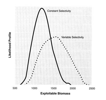
FIGURE 4.9 Estimates of uncertainty about management parameters derived from simple assessment models will be too optimistic if many of the assumptions are oversimplifications deliberately imposed to stabilize parameter estimates. Allowing for departures from the assumption of constant selectivity in this example leads to much wider probability profiles around estimates of exploitable biomass produced with a simple catch-at-age model (i.e., greater uncertainty).
- relative probability. The weight of evidence is formally the Bayes posterior probability, which is increasingly being used in fisheries assessments (Walters, 1986; McAllister et al., 1994; Raftery et al., 1995; Punt and Hilborn, 1997).
- Identify each alternative management action.
- Evaluate the distribution and expected value of each performance measure, given the management actions and the hypotheses.
- Present the results to decision-makers.
When there are a discrete number of alternative hypotheses and management actions, a "decision table" is an effective tool to summarize the decision analysis process and to present the results to decision-makers. The example shown in Table 4.2 contains the following:
- Alternative hypotheses about the true unexploited biomass level
- Probabilities assigned to each hypothesis
- Alternative management actions (TAC levels)
- Consequences (in terms of some performance measure) of alternative actions (given in the body of the table)
- Expected value of each management action (listed in right-hand column)
It is often possible to specify several different measures of population dynamics and stock condition as alternative hypotheses, and separate decision tables must be produced for each.
Decision tables have the advantage that scientists and managers must explicitly examine alternative hypotheses about stock condition or population dynamics, the probability of these conditions, alternative actions, and their consequences. Decision tables are limited in the number of different states of nature that can be considered, however; in models with several uncertain parameters, all of the alternative conditions cannot be shown together, yet they must be integrated across stock conditions to produce summary statistics such as expected value and distribution of outcomes for each management action.
TABLE 4.2 A Simple Decision Table to Evaluate the Consequences of a Variety of Alternative Annual Total Allowable Catches (TACs)
|
|
Alternative Hypothesis (unexploited biomass in thousand tons) |
Expectation |
|||||
|
|
750 |
950 |
1150 |
1350 |
1550 |
1750 |
1046 |
|
Probability |
0.099 |
0.465 |
0.317 |
0.096 |
0.020 |
0.003 |
|
|
TACa (thousand tons) |
|||||||
|
100 |
0.51 |
0.63 |
0.70 |
0.75 |
0.78 |
0.81 |
0.66 |
|
150 |
0.26 |
0.45 |
0.56 |
0.63 |
0.69 |
0.72 |
0.49 |
|
200 |
0.22 |
0.26 |
0.42 |
0.52 |
0.59 |
0.64 |
0.34 |
|
a Shown in the interior cells of the table as ratio of stock size at end of management period to unexploited biomass. SOURCE: Hilborn et al. (1994) Biomass expectation = σ Unexploited biomassi × Biomass probabilityi TAC expectation = σ Unexploited biomass probabilityi × TAC probabilityi |
|||||||


