
Hydrodynamics in Advanced Sailing Design
J.Milgram (Massachusetts Institute of Technology, USA)
Abstract
A review of up-to-date methods for incorporating the results of hydrodynamic studies in the sailing vessel design process is given. It is shown that a requirement for design evaluation is a Velocity Prediction Program (VPP) which simultaneously accounts for all the effects of design features and their variations. The need for experimental data, both for sails and hulls, as starting points in the design process is emphasized. Such data includes interactions which cannot be fully evaluated by numerical hydrodynamics. Much emphasis is given to the use of numerical hydrodynamics for refining design variations. Existing procedures in areas including wave resistance, lift and induced drag of appendages, and resistance due to sea waves are reviewed, and their roles in the design process are evaluated. New procedures and results in the areas of viscous flow over appendages, thrust due to unsteady motions and sail aerodynamics with influence of the hull beneath the sails are given.
1
Introduction
Development of sailing vessels began as a full scale trial and error process and still is, to a large extent. The first “research” done in a different way was scale model testing. Although ship model testing has been conducted for over 500 years, the process was not put onto the firm scientific basis of dimensional analysis until the work of William Froude beginning in 1868. The science and art of ship model testing has advanced considerably in the last 128 years. However, during most of this time the commercial and naval ships being developed were driven by propellers, not by sails. Therefore matters involving heel, side force and leeway have not been in the mainstream of developments in model testing. Instead, these specialties have been developed by those naval architects and ship hydrodynamicists involved with advancing the state of the art of sailing yachts.
Another aspect of hydrodynamic development for waterborne vessels is numerical hydrodynamics. Similar to model testing, the mainstream in numerical ship hydrodynamics relates to ships whose mean operating condition does not involve substantial side forces, heel angles or leeway angles. Again, these specialties have occupied the efforts of people involved with sailing yachts.
Almost all the experimental and numerical hydrodynamics used for ships driven by propellers has application to sailing vessels. Although the application of propeller hydrodynamics may seem remote when viewed superficially; there are, in fact, many similarities between them and numerical sail aerodynamics. The addition of the unique hydrodynamics of sailing vessels to the those that apply to all ships results in the complex aero/hydrodynamical system that is our subject here.
The development of numerical and experimental methods for advanced sailing vessel hydrodynamics has been stimulated almost entirely by the design of sailing craft for participating in some sort of speed contest. Although much of the development of such vessels is done by the usual trial and error process, the advantages of very small increments in speed have brought all resources to bear on the design of these craft. The most common type of contest is a yacht race whose distance can vary from several hundred meters to a circumnavigation of the globe. Most of these races are for monohulled craft, although a number of them involve multihulled craft. A less common contest is a time trial where the goal is to set a speed record. Long distance time trials involve vessels that are similar to those used in yacht races whereas short distance time trials involve a broader
range of craft geometries. In fact, in recent times the world sailing speed record has been held by a sail-board for which a significant component of the sail force is vertically upward.
The focus here is on the aero/hydrodynamics used in support of the design of monohulled yachts. However, several of the approaches have application to the less common sailing craft mentioned above.
The history of aero/hydrodynamic research related to sailing vessels can be divided into two categories. The first is the set of individual research programs of varying intensity and longevity whose modern history covers more than 50 years. The second category is the applied hydrodynamic research on sailing vessels stimulated by competition in the America's Cup yacht races. These events, typically held once every 3 to 5 years, have attracted extraordinary and unique international interest and intense competition. As a result, very substantial resources have been applied to every known way to increase the sailing speed of vessels which meet the specified requirements for the competition. Applied aero/hydrodynamic research is one of them. Most of the material to be presented herein is drawn from this category.
2
Evaluation of Designs and Design Ideas
Since a sailing vessel is a complex interconnected “system”, most design changes influence more than one kind of fluid force. For example, suppose one wishes to reduce the frictional resistance of the hull by reducing its wetted surface. For most hull shapes, if length is maintained, the reduction in hull wetted surface requires a reduction in beam. This in turn reduces the heeling stability which, for prescribed sail shapes, leads to an increase in heel angle. The change in heel angle not only changes the hull shape, but also changes the sail forces. How does one determine whether the sum of all these effects is advantageous or disadvantageous? More importantly, how can one evaluate the effects if the sail shapes are simultaneously changed to optimize them for the altered hull? Short of complete full scale sailing experiments, answering these questions must be done with a numerical method of predicting performance. A computer program that does this is called a Velocity Prediction Program (VPP). One can think of a VPP as ”sailing a boat in the computer”.
2.1
Fundamental Principles for a Velocity Prediction Program
The primary purpose of a velocity prediction program is to predict the boat speed for any prescribed wind conditions and sailing angle, βT, between the wind direction and the course of the boat. This is achieved in a computational model by balancing counteracting aerodynamic and hydromechanic forces and moments. The course of the vessel differs from the heading of its centerline by the yaw (leeway) angle, λ.
A few preliminary definitions and descriptions are needed before proceeding further. The true wind speed varies with the distance, z, above the water. Here, we will consider logarithmic wind velocity profiles described by:
(1)
where V10 is the wind speed at a height of 10 meters and zo is the roughness height which is taken here as 0.001 meters (1 mm). Hence the wind velocity profile v(z) is described by the single parameter V10. The deck plane is defined as a plane perpendicular to the centerplane of a vessel. Figure 1 shows the aerodynamic and hydromechanic force and moment components in the deck plane. Those involved in the VPP force and moment balance are:
Faf, the aerodynamic forward force in the course direction,
Fah, the aerodynamic heel force which is perpendicular to the forward force and the parallel to the deck plane. The aerodynamic force is presumed to be parallel to the deck plane. Thus the aerodynamic forces perpendicular to the deck plane are neglected in our model for evaluating performance here,
Mah, the aerodynamic heeling moment whose vector is along the centerline of the yacht,
Fwr, the resistance of the yacht in the direction opposite to the course direction,
Fwh, the hydromechanical force component which is perpendicular to the course and parallel to the deck plane, Fwh is exclusive of components of that part of the buoyancy force which balances the weight of the yacht.
Mwh, the righting moment of the water on the yacht. Its vector is in the direction of the yacht centerline. It includes both hydrostatic and hydrodynamic components.
For any equilibrium sailing condition there are three “balance equations” involving these forces and mo-
ments:
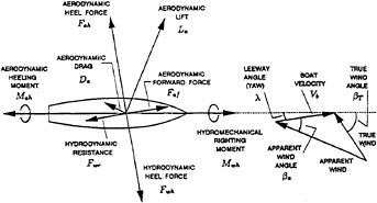
Figure 1: Forces and moments in the Deck Plane.
(2)
where Vb is the boat speed in the direction of the course, ![]() is the heel angle and λ is the leeway (yaw) angle.
is the heel angle and λ is the leeway (yaw) angle.
For prescribed values of the wind speed, V10, and the sailing angle βT, all six terms in equations 2 depend on the boat speed, the heel angle and the leeway angle. There are three equations for these three unknowns. The VPP solves the three equations for the three unknowns. Figure 2 is a block diagram of the VPP model.
Although solving the balance equations 2 is computationally intensive because the equations are nonlinear and the solution variables are intrinsic to the expressions, each related numerical step is precise and any desired level of numerical accuracy can be achieved. On the other hand, modeling all the forces involved is an approximate and imperfect science. Hydrodynamics, as we do it in terms of theory, experiment and numerical computation, makes its greatest contribution to this field by predicting forces and teaching us how to model them.
In addition to the basic force models, two additional VPP features, which involve feedback, are shown in Figure 2:
The Sail Shape Optimizer adjusts the sail shapes, and therefore their aerodynamic characteristics, so as to maximize the boat speed for the prescribed wind speed and direction.
The Direction Optimizer is activated for sailing upwind or downwind. Then, the best speed made good (VMG) occurs when sailing in a direction different from the direct path between end points. Tacking or gybing is done so as to achieve the net desired course with all the sailing done at the optimum wind angle.
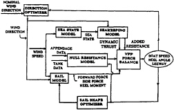
Figure 2: A Block Diagram of the VPP. This emphasizes the fact that solving the force balance equations is the minor and more ordinary part of the process. The modeling of the forces is necessarily imperfect and requires most of the effort in developing a faithful VPP.
2.2
An Example of Use of A Velocity Prediction Program
As an example of using a VPP, Figure 3 shows the effect of a 1% change in total resistance of an International America's Cup Class (IACC) yacht on time required to sail a course of 17.2 km upwind and 17.2 km downwind.
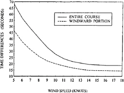
Figure 3: Time Differentials in Sailing a 34.3 km Course Due to a 1% Change in Resistance.
This example has been chosen not only to show one capability of a VPP, but also to demonstrate that requirements for performance prediction accuracy are extraordinary when optimizing the designs of racing yachts. A 1% change in resistance corresponds to a change in race course sailing time of 25 to 45 seconds depending on the wind speed. These times themselves relate to substantial margins of victory or defeat. When the tactical advantages of the faster boat are considered as well, the influences of the speed differences are even greater.
The time differentials shown in Figure 3 correspond to about 0.3% in the sailing time and in the average speed. In ordinary applications of naval architecture speed variations of 0.3% are negligible. If a new ship on trials deviates from her design speed by 0.3% (for example, 15.95 instead of 16 knots) it makes little difference. However, for racing vessels 0.3% is more than the difference between a true winner and an “also ran.” Even smaller speed differences can be meaningful so differences of very small magnitude need to be considered not only in designs, but also in methods of evaluating designs.
It is not possible to predict absolute boat speeds for a prescribed design to within 0.3% of the actual sailing speed, let alone the even smaller variations that are significant. However, this extreme accuracy is not required on an absolute basis. It is required on a relative basis and this can be achieved, to a greater or lesser degree depending on the design area under consideration, if the technology is pushed to its limit.
3
The Design Process
The design of a specific vessel needs initial data on what is always an incomplete relationship between performance and design parameters for similar vessels. Often, this comes from qualitative or semi-quantitative information from racing performance in competitions in which vessels of varying designs compete. Although it is the most common information source, such data suffers from being in a form which makes it impossible to separate hull hydrodynamics, sail aerodynamics and sailing ability of the crew.
At its best, initial data on the relation between hull geometry and the hydrodynamic aspects of performance come from towing tank model tests, supplemented by numerical results on the added resistance in sea waves as it is very difficult to determine this experimentally with sufficient accuracy. Ideally, initial tank tests results include a series of models with systematic variations of design parameters. Although systematic data is most helpful to hydrodynamicists in developing improved designs, projects which acquire model test data are almost always under pressure to conduct tests on all the latest design ideas or one designer's “breakthrough brainstorm.” It takes unusual discipline and substantial resources in a design effort to acquire initial data on systematic parametric variations.
No matter how the initial data is obtained or the form it takes, the next step is to try to achieve design improvements. In addition to the “artistic” approaches used by many naval architects and yacht designers, this is the stage where quantitative theoretical, numerical and experimental hydrodynamics can make significant contributions. It is especially helpful to have systematic model test data at this stage since it provides a basis for comparison with the results of numerical hydrodynamics. If the later is verified by comparison with experiments, it can be used with more confidence in exploring new designs.
A significant technical management effort is required to integrate the initial data, the artistry of the traditionalists and the findings obtained by hydrodynamics. The goal is to achieve one or more improved designs. If the time has come to build a new design and if one of the new designs is an improvement over the starting designs, the best one can be chosen. However, if the development process is to continue further, it is best to conduct model tests on systematic variations of the new best design and repeat the process.
4
Decomposition of the Force Components
A vessel under sail with non-zero heel and yaw angles is a complex interrelated system. The exact situation is one in which the water flow around the hull is not symmetric, port and starboard, due to the heel and yaw; and the air and water flows influence each other. It is necessary to make simplifying approximations; not only to be able to apply the present state-of-the-art in hydrodynamics, but also to be able to achieve a practical design process.
The first simplifying approximation is that the air and water flows do not influence each other. In other words, the coupling between air forces and water forces is approximated as being wholly mechanical (the rig and the hull are structurally connected) and not hydrodynamical. This is not to say that the optimum aerodynamic design is independent of the optimum hydrodynamic design. In fact, since different hulls require different sails for optimum performance, these optima are closely coupled. Rather, it is to say that for any prescribed geometry and sailing conditions the aerodynamic and hydrodynamic flows are determined independently.
4.1
Hydrodynamic Resistance
The essential goal in modeling hydrodynamic resistance is determination of the function Fwr(Vb, ![]() , λ), or alternatively Fwr(Vb,
, λ), or alternatively Fwr(Vb, ![]() , Fwh), for any prescribed hull form in prescribed sea conditions. A useful approach is to use an additive resistance model of the following form:
, Fwh), for any prescribed hull form in prescribed sea conditions. A useful approach is to use an additive resistance model of the following form:
Fwr=Dhf+ Dr+ Daf+ Dhi+ Dw–Tu (3)
where:
Fwr is the total hydrodynamic resistance (drag),
Dhf is the frictional drag of the hull,
Dr is upright residuary resistance of the entire vessel,
Daf is the friction and interference drag of the appendages,
Dhi is the drag due to heel and yaw (leeway), or equivalently, due to heel and heel force production,
Dw is the resistance due to sea waves (added resistance), and
Tu is the mean dynamic thrust due interactions of appendages with the unsteady flow resulting from vessel seakeeping motions and sea wave orbital velocities.
Usually, non-dimensional force coefficients, C,
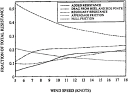
Figure 4: Fractions of Total Resistance for Each Component for Upwind Sailing
are obtained by dividing corresponding forces by ![]() where ρw is the density of the water, Vb is the boat speed and Sh is the wetted surface. It is sometimes useful, particularly in wind tunnel model testing, consider “force areas”, A, obtained by dividing corresponding forces by
where ρw is the density of the water, Vb is the boat speed and Sh is the wetted surface. It is sometimes useful, particularly in wind tunnel model testing, consider “force areas”, A, obtained by dividing corresponding forces by ![]() where ρ is the density of the test fluid and V is the relative inflow velocity.
where ρ is the density of the test fluid and V is the relative inflow velocity.
Figure 4 shows the fraction of resistance contributed by each component, exclusive of Td, vs. wind speed from VPP computations for an IACC yacht using tank test data and measured sea spectra in San Diego California as inputs. Figure 5 shows the fractions for sailing downwind. Tacking angles for optimum speed made good are used both upwind and downwind.
The hull friction is always the largest component for upwind sailing and it is largest for downwind sailing in wind speeds less than 12 knots. For higher wind speeds in downwind sailing the residuary resistance becomes the largest because of the high boat speeds in these conditions. The effects of resistance due to heel, side force, and added resistance are negligible in downwind sailing and are neglected in Figure 5. The reader needs to be aware that the relative merits of two boats sailing downwind in large seas are also influenced by the relative surfing ability, and that is not included in the computations. For upwind sailing, in the mid-range of wind speeds, all the other resistance components are comparable to each other. At very low wind speeds the appendage friction is largest component after hull friction. The boat speed is low enough in these conditions for the residuary resistance to be considerably smaller than the appendage friction, and the sea waves are small enough for the added resistance to be small as well. On the other hand, at high wind speeds the combi-
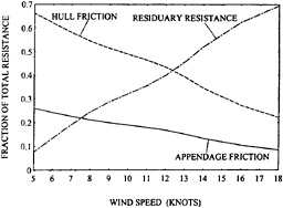
Figure 5: Fractions of Total Resistance for Each Component for Downwind Sailing.
nation of boat speed, sail side force, and sea waves makes the residuary resistance, resistance due to heel and side force, and added resistance similar and large enough for the fraction due to appendage friction to be somewhat less. This exercise is one demonstration of the requirement for using velocity prediction programs. The increase in fraction of residuary resistance with increasing wind speed is due to the increase in boat speed with wind speed. However, the ratio of sail side force to the square of the boat speed increases and this is why the fraction of resistance due to induced drag increases as well.
Strictly speaking, the terms in equation 3 are not independent of each other. For example, the viscosity, which is mainly responsible for friction drag, causes boundary layers whose displacement thickness influences the residuary wavemaking resistance. Similarly, the ship-generated waves cause pressure gradients along the hull which influence the boundary layers and the associated friction drag. If each term in equation 3 is determined or estimated independently of the others, the interactions between terms are not accounted for. However, if scale model tests are conducted the interactions are captured if the model scale is not too small. They get mixed into the various terms in the decomposition. For example if the upright residuary resistance is defined as the measured resistance minus the presumed frictional resistance, the sum of these two resistances automatically includes the interactions. The work of Kirkman and Pedrick (1974) suggests that scale model waterline lengths need to be 5 meters or more for there to be a reasonable assurance of reliable results in the experimental process and expansion of its data to full scale.
Once a set of resistance components which includes their interactions are determined by model testing, it is often quite useful to use numerical methods to estimate the difference in one of the resistance components between two designs. Although this may not capture differences in the interactions, it often provides a good approximation to the differences that are the most significant. Some of the numerical methods in use will be considered in the sequel here.
4.2
Aerodynamic Forces
The forward and heeling aerodynamic forces, Faf and Fah, are given in terms of the aerodynamic lift and drag forces, La and Da, and the apparent wind angle, βa, as:
Faf=La sin βa–Da cos βa (4)
Fah=La cos βa+Da sin βa (5)
Similarly, the aerodynamic heeling moment, Mah, is determined from these forces and the heights of their centers.
On a moving vessel, the apparent wind speed and angle depend on height since the components due to true wind speed depend on height and the component due to vessel speed is independent of height. Some height must be chosen for a reference apparent wind speed, Va, and a reference apparent wind angle, βa. Here the reference height will be taken as 10 meters above the water.
The lift force, La, can be quite accurately determined from lifting surface theory (c.f. Greeley et al., 1989 and Milgram, 1968) for upwind and close reach sailing where the local sail cambers and incidence angles are modest. For offwind sailing, flow separation is almost always large enough to materially influence the lift so that experimental data are required to “construct” a mathematical model for it.
The aerodynamic drag force includes the induced drag of the sails as well as the frictional and parasitic drag on the sails, mast, rigging and hull. For windward and close reach sailing, the induced drag data can come from the same computational implementation of lifting surface theory that provides the lift. However, all the drag for off wind sailing and the friction and parasitic drag for upwind sailing must come from experiments or empirical estimates.
Aerodynamic lift and drag coefficients, ![]() and
and ![]() are taken as:
are taken as:
(6)
where ρa is the air density and Sa is the actual sail area.
Each sailing condition has a different lift and drag coefficient for optimum performance. The usual modeling approach is to determine a maximum allowed lift coefficient as a function of apparent wind angle, ![]() For each apparent wind angle and operating lift coefficient, which can be any positive value less than or equal to
For each apparent wind angle and operating lift coefficient, which can be any positive value less than or equal to ![]() there is an associated drag coefficient. The VPP also needs to choose the amount of sail area to set, up to a maximum allowed amount, for optimum performance. To complete the specification, the drag coefficient needs to be “modeled” as a function of CL and βa.
there is an associated drag coefficient. The VPP also needs to choose the amount of sail area to set, up to a maximum allowed amount, for optimum performance. To complete the specification, the drag coefficient needs to be “modeled” as a function of CL and βa.
The author has had success in modeling the drag coefficient as:
(7)
where:
![]() includes the friction drag of the sails and the profile drag coefficient of the hull, mast and rigging,
includes the friction drag of the sails and the profile drag coefficient of the hull, mast and rigging,
Ci(βa) is a coefficient of induced drag, and
![]() is a coefficient of lift-dependent profile drag.
is a coefficient of lift-dependent profile drag.
The last two terms in equation 7 are proportional to the square of the lift coefficient so one might ask why they are not combined into one. The reason is that for a given lift coefficient the induced drag is particularly sensitive to aspect ratio and vertical distribution of lift, whereas the profile drag is less sensitive. Therefore, by keeping the terms separate, a model for one sailplan can be adjusted for a change in vertical lift distribution (Euerle and Greeley, 1993) or used to model a different sailplan by altering Ci in ways that can be well approximated theoretically.
Two approaches can be taken for estimating ![]() and
and ![]() One is to add estimates of the drags from hull, mast, rigging and sails, with each determined as well as possible from existing data. As examples, rigging drag can be based on published drag coefficients for cylinders and sail parasitic drag can be based on section data (Milgram, 1971). The other approach is to measure the drag and subtract the induced drag computed from lifting surface theory for the sail shapes in use to obtain the other drag components. This has been done by the author (Milgram, 1993) by using an instrumented sailing vessel for measuring aerodynamic forces.
One is to add estimates of the drags from hull, mast, rigging and sails, with each determined as well as possible from existing data. As examples, rigging drag can be based on published drag coefficients for cylinders and sail parasitic drag can be based on section data (Milgram, 1971). The other approach is to measure the drag and subtract the induced drag computed from lifting surface theory for the sail shapes in use to obtain the other drag components. This has been done by the author (Milgram, 1993) by using an instrumented sailing vessel for measuring aerodynamic forces.
5
Towing Tank Testing
A complete consideration of the towing tank testing of model scale sailing vessels will not be presented here as it is well covered in the literature (c.f. Van Oosannen, 1993 and Milgram, 1993). Rather, the process is outlined and some special problems are described.
When data are obtained by model testing, the frictional terms, Dhf and Daf, are subject to Reynolds scaling whereas the other terms, Dr, Dhi and Dw, are considered to be subject to Froude scaling. The upright quantities, hull friction, appendage friction and residuary resistance are determined in the same way in ordinary resistance tests of vessels that are not powered by sails. Appendage friction is estimated on the basis of appendage geometry and the hull friction coefficient is taken as:
Chf(Re)=(1+k)Cf(Re) (8)
where:
Re is the Reynolds number based on length,
k is the form factor evaluated from the tank data by the method of Prohaska (1966), and
Cf(Re) is the “flat plate” frictional resistance.
The difference between the measured resistance and the estimated frictional resistance is taken as the residuary resistance, Dr.
In addition to straight ahead tests with the vessel upright, a sailing vessel model needs to be tested with non-zero heel and yaw (leeway) angles with both resistance and side force measured. This greatly increases the number of tank runs required for a sailing vessel as compared to an engine-propelled vessel. In the author's experience, about 135 test combinations of speed, heel and leeway are required to fully quantify the hydrodynamic forces on a sailing vessel.
In conducting tank tests of vessels to be used for racing, accuracy and repeatability are of paramount importance. Section 2.2 describes the sensitivity of racing performance to small changes in resistance. Since total accuracy is impossible, a reasonable approach is to strive to limit measurement errors or lack of repeatability to 1% or less and to take special measures when one has to choose between designs whose predicted performances differ by less than the amount associated with a 1% change in resistance. For example, the scale model of each design can be tank tested at four separate times and the results then averaged together. This reduces the erroneous data variability by a factor of 2.
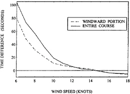
Figure 6: Performance Prediction Comparison Based on Two Test Sequences on the Same Yacht Model.
It is not easy to obtain this 1% level of accuracy and repeatability. Although state-of-the-art instrumentation can measure the forces, model orientations and speeds with the desired accuracy, variable fluid motions due to thermal stratification and from circulation patterns in many towing tanks can lead to errors larger than the set limit. It is common to “stir” tanks with several high speed runs generating breaking ship waves and then to wait until surface currents measured by small floats are sufficiently small before conducting a test sequence. Then, to make comparative results between similar designs as accurate as possible, the exact same test run sequence with the same timing of runs is used for all models. Nevertheless, the errors are still sometimes excessive. Figure 6 shows the difference in performance prediction from two separate model test sequences done several weeks apart on the same IACC yacht model in the same facility, using the aforementioned precautions and carefully calibrating all measurement instruments before the sequence and checking to be sure the calibrations are unchanged at the end of the sequence. The model waterline length is about 6 m, which is thought to be large enough. Yet, for this case errors in excess of the desired limit exist. Dr. Bruce Parsons (Private communications, 1995 and 1996) has told the author that the 1% repeatability error limit on forces is met by tests he conducts in a different facility. As yet, we do not know why a difference in repeatability of measured data exists in the different facilities.
6
Individual Components of Resistance
This section focuses on the components of resistance individually, with emphasis on numerical methods for estimating some of them. As was previously described, existing numerical methods are not physically complete enough for the sum of the resistance components to yield speed predictions which are precise on an absolute basis. However, numerical methods for some of the resistance components are useful for comparing design differences.
6.1
Hull Friction
Although hull friction is often the largest of the resistance components, it is the one that is least amenable to numerical hydrodynamics. Similarly, systematic experimental studies of the relationship between sailing vessel hull parameters and the friction drag coefficient have not been done, at least to this author's knowledge.
At the present state-of the-art, a meaningful experimental program would be extensive and difficult. The essential difficulty in conducting experiments to relate hull friction drag to hull form parameters is determination of the friction drag in the experiments. It could be based either on flow measurements or force measurements.
The approach using flow measurements would be to examine the momentum flux in the central portion of the wake. A complication is that some of this momentum flux is associated with the ship waves and this needs to be subtracted from the total measured momentum flux. One possibility is to determine the wave field in the wake by a “wake cut analysis.” Another is to compute the wave field numerically. This computation would not be precise because of limitations in the state-of-the-art for such computations and because the influence of the boundary layers on the ship-generated wave field is not known precisely. However, they might be good enough for this purpose. It is a possibility worth considering.
A similar problem exists if the friction drag is to be determined from force measurement. The wavemaking drag would have to be subtracted from the measured drag. The aforementioned statements about determining the wavemaking drag from “wake cut height measurements” and from using numerical computation apply here too.
Without either a robust numerical tool or an experimental “data base” for friction drag, towing tank
experiments with the friction drag estimated by Prohaska's method is the state-of-the-art. This cannot estimate the friction drag precisely since it yields a coefficient that depends only on the Reynolds number whereas there are Froude number effects on the friction drag. Thus the error in the estimate gets mixed into the other resistance components which are all subject to Froude scaling, except for the appendage friction. This is one reason why tank test models must be large.
Development of numerical methods for calculating hull friction is currently being pursued as an area of research. Some RANS codes show promise and extension to free surface flows of the integral boundary layer equation method described subsequently for appendages is an exciting possibility.
6.2
Computation of Viscous Drag on Appendages
Appendages on a fin keeled sailing vessel include the keel fin and the rudder. There may also be a ballast bulb and the keel or the rudder, or both, might have winglets. One underwater profile showing such appendages is shown subsequently in Figure 15 The rudder and keel fin and optional winglets are typically high aspect ratio lifting surfaces so there is reason to examine their friction drag from the basis of two-dimensional section analysis. This will be discussed here, first for clean water. Then brief speculations about the influences of particulate matter and small gas bubbles in the ocean will be given.
The goal for numerical hydrodynamics of airfoil sections is prediction of lift, drag and moment coefficients for a prescribed angle of incidence and Reynolds number, which is based on the chord length for the sections. The problem involves a largely inviscid outer flow away from the immediate vicinity of the airfoil and boundary layers adjacent to it. For many years people tried to iterate between the inviscid and boundary layer solutions. The idea was to compute an inviscid flow, use its pressure gradients in solving the integral boundary layer equations, re-solve for the inviscid flow with the airfoil “thickened” by the displacement thickness of the boundary layer, including the viscous wake, re-solve the boundary layer equations, etc. This approach failed when the boundary layer thickened rapidly, even for very small amounts of flow separation close to the trailing edge.
Over the past several years, ingenious schemes for solving for the outer flow and the boundary layer flow simultaneously and with tight coupling have been developed. They have been extraordinarily successful in providing predictions in close agreement with experiment. Examples are the developments of Eppler and Somers (1980) and Drela and Giles (1987) (see also Drela, 1989). These schemes contain a mix of mathematically precise panel methods and integral boundary layer equations, and empirical or semi-empirical relations that relate various boundary layer parameters.
An outline of a method similar to that of Drela (1989) is presented here. The only significant difference is that Drela cast the outer inviscid flow in terms of its stream function and the presentation here is the form used by W.Milewski (1996) in terms of the velocity potential continued onto the airfoil surface, ![]() , which is represented as:
, which is represented as:
(9)
where:
G is the two-dimensional Green Function, log r,
n is the normal into the airfoil surface,
sb is the path around the airfoil,
sw is the path along the centerline of the wake,
Δ![]() w is the jump in potential across the wake from top to bottom. It is constant along the entire wake, and
w is the jump in potential across the wake from top to bottom. It is constant along the entire wake, and
σ is a ficticious “transpiration” source strength distribution along the airfoil surface and wake that has to be determined so as to make the outer flow the same as the real boundary layer would cause.
The left hand side and first two integrals on the right hand side of equation 9 comprise the ordinary application of Green's theorem for inviscid lifting flows and the last integral simulates the effect of the boundary layer displacement thickness on the outer flow. The discretized form of equation 9 with the usual summation convention is:
(10)
Here, the panels on the airfoil start with number 1 at the trailing edge on the bottom, go around the foil and end with number N at the trailing edge at the top. The Ci coefficients include the integral of ![]() over the entire wake. In this form, equation 10 is strictly valid only if the vector between control points 1 and N is orthogonal to the incident velocity
over the entire wake. In this form, equation 10 is strictly valid only if the vector between control points 1 and N is orthogonal to the incident velocity
vector. Otherwise, ![]() is subtracted from the left hand side since it contributes to Δ
is subtracted from the left hand side since it contributes to Δ![]() w (c.f. J.T. Lee, 1987).
w (c.f. J.T. Lee, 1987).
The left hand side can be combined with the second, third and fourth terms on the right hand side to obtain:
(11)
where:
Aij=πδij+Aij+(δjN–δj1)Ci (12)
and
(13)
Multiplying all terms by ![]() gives:
gives:
(14)
The first term on the right hand side is the perturbation velocity potential for the inviscid flow around the airfoil, which will be called ![]() inv. The second term is the contribution to the outer flow potential from the existence of the boundary layer as represented by the transpiration sources. Equation 14 is then written as:
inv. The second term is the contribution to the outer flow potential from the existence of the boundary layer as represented by the transpiration sources. Equation 14 is then written as:
(15)
The total potential, Φ, is the sum of the perturbation potential and the free stream potential, ![]() inf,
inf,
(16)
The surface velocity, which corresponds to the tangential velocity at the outer edge of the boundary layer is called Ue, and is obtained as the derivative of the total potential with respect to the tangential coordinate, s.
(17)
(18)
The mass defect in the boundary layer, M, is related to the displacement thickness, δ*=∫(1–u/Ue)dη (η is the coordinate normal to the surface) and the transpiration source strength by:
(19)
(20)
By substituting equation 20 into equation 17 and collecting terms that multiply each element of mass defect, Mj, equations of the following form are obtained:
(21)
(22)
D is a known matrix. The objective is to find a solution for M and the other boundary layer parameters that satisfy the integral boundary layer equations:
(23)
(24)
where:
θ≡∫(u/Ue)(1–u/Ue)dη is the momentum thickness,
H≡δ*/θ is the shape parameter,
Cf≡2τwall/[ρ(Ue)2] is the skin friction coefficient,
θ*≡∫(u/Ue)([1–(u/Ue)2]dη is the kinetic energy thickness,
H*≡θ*/θ is the kinetic energy shape parameter,
CD≡∫τ(du/dη)dη/[ρ(Ue)3], and
τ is the shear stress and u is the local velocity in the boundary layer.
In addition to equations (23, 24) a third equation is used. The third equation is an empirical one, based on correlations with boundary layer measurements, and is different for laminar and turbulent boundary layers. For the laminar case, the ratio of the amplitude of the most unstable Tolmein-Schlichting wave at any chordwise location to its ratio at the leading edge is expressed as ![]() The empirical equation is:
The empirical equation is:
(25)
where f1 is an empirically determined function of H and θ. The user must specify either the location of the point of transition from laminar to turbulent flow or the value of n for which this occurs. In flows of clean fluids, the transition value of ñ depends on the turbulence level of the incoming stream. Mack (1977) gives this value as:
n=–(8.43+2.4 log Tf) (26)
where Tf is the ratio of the rms turbulence speed to the free stream speed.
For a turbulent boundary layer, an empirical equation for the spatial derivative of the maximum shear
stress coefficient, Cτ, in the following form is used:
(27)
For any location on the airfoil, specification of θ, M, and Ue provides all the other boundary layer parameters in laminar flow through empirical and semi-empirical relations which can be found in Drela and Giles (1987). For a turbulent boundary layer, values of θ, M, Cτ and Ue are required to obtain all the other parameters (θ*, δ, Cf, CD).
The approach for a prescribed distribution of Ue, which is taken as the inviscid solution for a starting point, is to iteratively determine values for the “independent parameters”, θ, M and Cτ (when needed), that solve equations 23, 24 and 27. Until the correct values for these quantities are obtained, the sum of the terms on the left hand sides of these equations will not equal zero. Newton 's Method is used to iterate on the independent parameters. The crucial feature, that makes the whole scheme work, is that at each iteration the distribution of Ue along the entire airfoil is changed according to the iterative changes in the Mj's and equation 22. Hence, as the boundary layer is altered toward correctness, iteration by iteration, the outer flow which generates the pressure distribution that drives the boundary layer is simultaneously altered toward correctness.
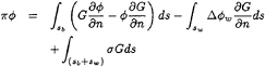
Figure 7 shows drag coefficient vs. lift coefficient for an airfoil section as calculated by this method using the program XFOIL (Drela, 1989) and as measured in the M.I.T. water tunnel. For the calculation, ñ was set to 3.5, which corresponds to the turbulence level of 0.7% which exists in the tunnel. Experimental forces were based on velocities around a large rectangle surrounding the section, measured with a laser doppler velocimeter, and applying the Bernoulli equation outside the wake and momentum conservation principles to the flow.
Figure 8 shows the airfoil section characteristics calculated by this method for two section shapes that could be used for the keel fin of a sailing vessel. One section has a thickness fraction of 0.13 and the other has a thickness fraction of 0.17. The calculation is done for ñ=9 which corresponds to an incident stream with negligible turbulence. The figure indicates that for lift coefficients in excess of 0.33 the thicker section has less friction drag. The reason for this is that the thicker section is predicted to have more laminar flow.
Design experience runs counter to this result. A boat goes faster with a keel thickness fraction of 0.13 than with a thickness fraction of 0.17. If one reduces ñ to
Figure 7: Calculated (line) and Measured Section Drag vs Lift Coefficients.
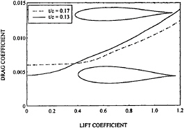
Figure 8: Section Characteristics for Two Airfoil Sections with a Clean, Low-Turbulence Inflow.
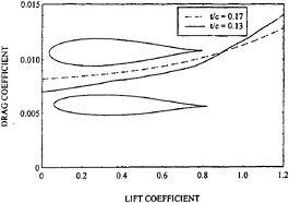
Figure 9: Section Characteristics for Two Airfoil Sections with Forced Suction Side Transition at 5% of the Chord.
3.5 which corresponds to a turbulence level of 0.7% (incoming rms turbulence of 3.5 cm/s with a boat speed of 5 m/s), the drag “crossover ” occurs at a lift coefficient of 0.6, but we know that for a boat with a keel fin operating at this lift coefficient the thinner keel is still better.
The reason for the disparity between the computed results and sailing experience could be that the combination of free stream turbulence, particulate matter and small gas bubbles in ocean water near the surface cause transition near the leading edge on the suction side —no matter what the section shape (c.f. Lauchle and Gurney, 1984).
Figure 9 shows the airfoil characteristics with suction side transition set at a maximum downstream location of 5% of the chord. For this forced transition condition, the thinner section has less drag up to a lift coefficient of 0.88. This is consistent with design experience as operating lift coefficients are designed somewhat lower than 0.88. The combined effects of free stream turbulence and particulate matter in the flow is an area in need of further study.
Milewski (1996) has extended the approach of coupling the integral boundary layer equations to inviscid panel methods, as described above, to three dimensional problems. The method provides the tangential friction drag and the normal pressure drag individually. Figure 10 shows these drag coefficients (based on surface area) vs. Reynolds number, as calculated by Milewski, for a form that might be used as the ballast bulb on a sailing vessel, with forced transition at 5% of the bulb length. It is an NACA 0020 section rotated to form a body of revolution. Coincidentally, the friction drag coefficeints are remarkably close to the ITTC friction “line”.
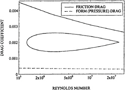
Figure 10: Drag Coefficient, Based on Bulb Area, for an Axisymmetric Ballast Bulb.
6.3
Residuary Resistance
The residuary resistance is the sum of the wavemaking resistance, interactions between resistance components that are not explicitly modeled, and errors in the presumed frictional resistance that get included in the residuary resistance by the resistance decomposition process. To the extent that these resistance components are influenced by the Reynolds number, errors in predicting full scale resistance from towing tank measurements are minimized by using large models. For example, with a one-third scale model of a 20 meter long vessel, if the frictional resistance is in error by 4% due to an error in estimated form factor, the full scale predicted resistance is in error by less than 1% at typical sailing speeds.
6.3.1
Numerical Methods
The most attractive possibility for the use of numerical hydrodynamics in minimizing residuary resistance is computation of the wavemaking resistance for differing hull geometries. As will be shown here, the state-of-the-art is not yet good enough to do this effectively in a design development program. However, it is getting better, and the routes to further improvements can be planned.
Although formal theoretical procedures for estimating wave resistance began almost 100 years ago with the thin ship theory of Michell (1898) and continued in several directions, including the slender ship theory of Tuck (1961), their level of accuracy did not approach one that could be considered for use in design until development of the method of Dawson (1977). . Whereas all the prior methods linearized the mathematical problem about the flat free sur-
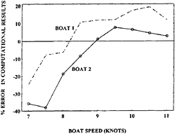
Figure 11: Percentage Error in the Wave Making Resistance Computed by Rosen et al.
face with a uniform stream, Dawson linearized the ship wave problem about the double-body flow which corresponds to the submerged portion of the ship beneath a rigid free surface. This basis flow contains many of the influences of the flow around the displacement form of the ship. Only the surface waves are left out and these are approximated as a linear perturbation on the double body flow. Both the basis double body flow and the perturbation wave flow are determined by a source or source and dipole based panel method using the Rankine source Green function.
Two notable extensions and applications of Dawson's method to sailing vessel hulls are those of Rosen et al. (1993); and of Nakos, Kring and Sclavounos (1993) (also described by Sclavounos, 1995). These approaches and their associated computer codes are the best we have today, but it will now be shown that they are not accurate enough to meet design requirements.
Figure 11 shows the percentage error in the numerical predictions of wave resistance in the upright condition for two different IACC hulls having identical appendages as measured from the figures in Rosen et al. (1993). The percentage error, E%, is defined as:
(28)
The difficulties in using numerical results in support of design are both absolute and relative. Absolute errors in wave resistance on the order ±20% correspond to time differences in sailing a 34.3 km windward-leeward course of ±2 minutes, a huge amount in match racing terms.
Figure 11 shows a difference in wave resistance error for the two designs of as much as 25%. Two caveats concerning these data need to be mentioned. The measured data were obtained by subtracting (1–k)CITTC from the measured total resistance coefficient, where CITTC is the ITTC friction coefficeint. An error in estimating the form factor, k, could cause an overall vertical shift in each curve. That notwithstanding, the data cannot provide design-level confidence since correction by a constant shift of one curve still leave excessive error differences over the important speed range.
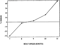
Figure 12: Percentage Error in the Wave Making Resistance of an IACC Yacht Computed by Sclavounos.
The second issue is that demands of their sponsoring organizations required that Rosen et al. omit scale numbers on the axes of their graphs for the case shown by dashed lines in Figure 11. This does not compromise the percentage errors since they are ratios. However, the location of each point on the abscissa is not precisely known. This author has assigned an abscissa scale on the basis of the wave resistance vs. speed characteristics for the type of vessel in question. It could be slightly in error, necessitating a slight shift or dilation in the abscissa location for the points on the dashed curve. However, this does not alter the conclusions about the results.
Figure 12 shows percentage wave resistance error vs boat speed for an IACC yacht as computed and presented by Sclavounos (1995). Again, the data here are scaled from a figure presented by Sclavounos and equation 28 is used.
Although the form and magnitude of the error is similar to the cases of Rosen, et al. there are a number of minor differences and one major one in the numerical methods which could be of importance when it comes to improving them. The approach of Scalvounos and his colleagues solves the initial value problem
in which the vessel is brought to speed from rest and the time domain computation is continued until the wave resistance becomes nearly steady. In this process, the surface elevation is computed at each time step. Due to the shallow slope profiles of the vessels under consideration, the wetted length changes throughout the computation. An artifice that is used is to stretch the vessel longitudinally at various time steps so the still water length matches the computed wetted length, followed by re-computing the double body basis flow. This was found to reduce the error between computation and measurements at the higher speed. Another artifice used by Sclavounos is to alter the boundary condition on some of the near-centerline free surface panels that border on the separation line of the stern underbody profile. Instead of using the usual kinematic free surface boundary condition on these panels, the condition of tangent separation was used inasmuch as this is what is observed on real vessels.
In spite of these special features in the numerical methods, they show considerable over-prediction of the wave resistance at high speed. Part of this in the Sclavounos method may be related to the fact that displacement is not preserved in the mathematical hull stretching process. It is well known to naval architects that wave resistance increases rapidly with displacement at high Froude numbers. Another potential source of the high speed error is the fact that the real flow and its forces are not a linear perturbation about the double body flow as is presumed in the computations.
6.3.2
Realities About the Resistance of Sailing Vessels
The progression of IACC sailing yachts whose design involved this author included those designated as USA 9 and USA 23. In nearly all conditions, the latter could sail a course of about 34 km two or more minutes faster than the former. Figure 13 shows the upright resistance drag areas determined by expanding towing tank test data to full scale. For all boat speeds less than 11.5 knots, the slower USA 9 is shown to have slightly less resistance. The total upright resistances predicted from model scale towing tank test data are very nearly equal for these two designs whose actual performances are quite different. The reasons for the difference in performance involve some smaller factors and one larger one. In this instance, the smaller ones include differences in heel stability and in the added resistance from sea waves. However, the largest difference involves the
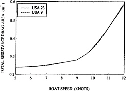
Figure 13: Total Upright Resistance Drag Areas for two IACC Yachts Predicted from Towing Tank Model Test Data.
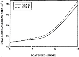
Figure 14: Total Resistance Drag Areas for Two IACC Yachts with a Heel Angle of 20 Degrees as Predicted from Towing Tank Model Test Data.
relative calm water resistances when the vessels are heeled. Figure 14 shows the drag areas vs speed, as determined from the tank tests, for the same two designs at a heel angle of 20 degrees and zero side force. Differences in resistance up to 4% are seen and the design with superior performance is the one with lower resistance. Of course, in actual sailing there would be non-zero side forces when the heel angle is 20 degrees, but the zero side force cases are shown here to show the effects of heel most clearly.
It is not at all uncommon for sailing vessels of differing performance potential to have similar upright resistances, but significantly different resistances when heeled. This fact is well appreciated by many yacht designers, but is often given insufficient consideration by marine hydrodynamicists and those naval architects that do not work with vessels that oper-
ate in the heeled condition. For example, most of the numerical predictions which have been made for sailing vessels are for the upright condition.
6.3.3
The Future for Numerical Evaluation of Residuary Resistance in Support of Design
Results from both towing tank and numerical experiments indicate a route that may lead to numerical methods for residuary resistance that can have greatly increased utility in the design process. First of all, present methods must be extended to the case of heeled vessels. This is a straightforward extension.
It is known that the increase in wetted length with increasing speed for sailing vessel forms with shallow slope overhangs must be accounted for. As described above, present day computations are done by solving the startup problem and waiting for a steady state to occur, with artificial adjustments to the hull shape at each time step. The natural extension is to do the startup problem for the fully nonlinear case, although there are complications. For example, the free surface panels will no longer lie in the still water plane and their locations will be time-dependent. At each time step, the computed wetted shape would be used instead of the artificial stretching. Thus, programs will be more complicated and require more computer resources. Convergence studies will necessarily be more complicated. However, there does not appear to be any major roadblock that would stop extension of the time domain panel methods for wave resistance to the nonlinear case.
Section 6.2 describes the ongoing work related to coupling inviscid panel methods with the integral boundary layer equations for determining forces on three-dimensional objects in the absence of a free surface. This method might be able to be coupled with future wave resistance calculations so as to get the frictional resistance and frictional-wavemaking interactions at the same time.
6.4
Induced Drag of the Hull and its Appendages
The form of resistance decomposition shown in equation 3 is chosen, in part, for convenience. The first three terms provide the calm water resistance in the upright condition, the fourth is the change due to the vessel operating at non-zero heel and leeway (yaw) angles and the fifth adds the resistance increase due to the presence of sea waves. The focus of this section is the use of theoretical and numerical methods for estimating a portion of the differences in the fourth term, the resistance increase due to heel and leeway, for different designs.
The portion under consideration here is the induced drag associated with the production of side or heel force. The induced drag occurs because the circulation around all side force-producing portions of the hull and appendages induces changes in the flow direction everywhere and the local lift is perpendicular to the induced flow direction. The induced flow is in exact analogy to the downwash of an airplane which is responsible for its induced drag.
The sailing vessel designer has a great deal of control over the induced drag because it is influenced in a minor way by variations in hull shape, and in major ways by variations in the appendages. These include keel fins, rudders, keel ballast bulbs and transverse winglets on keels, rudders or both.
In theory, the induced drag of a lift (heel force) producing object is very nearly proportional to the square of the lift for flows in the absence of a free surface. However, towing tank tests show that the actual induced drag vs. lift2 function of a sailing vessel differs from the theoretical one based on no free surface, both in its mean slope and in its linearity. Examples can be found in Greeley and Cross-Whiter (1989). The disparity is certainly related to free surface effects, although it is likely that some nonlinearity is due to the leeway-dependent location of the aft stagnation zone on the heeled hull.
Completely numerical determination of induced drag for use in speed prediction at the required level of accuracy for racing vessels is beyond the state-of-the-art. It awaits development of robust numerical methods that accurately solve for the heeled and yawed entire vessel, including both the boundary layers and the largely inviscid outer flow. However, there is good reason to believe that presently available numerical hydrodynamics can evaluate the difference in induced drag between identical canoe-body hulls with different appendages. The approach used is to solve for the inviscid flow about the heeled and yawed wetted portions beneath a rigid free surface. In practice, this is done by solving for the double body flow in an infinite fluid. Reasons justifying this approach include:
-
The free surface effects on the side force and induced drag are strongest on the canoe body. With the same canoe body used in comparisons, the difference in these effects due to appendage variations should be small.
-
Most of the hull-induced flow variations on the appendages are due to the hull displacement effects, which are captured in the rigid free surface problem. The ship wave flow effects on the appendages, which are not included in the rigid free surface problem, are very nearly the same when only the appendages are varied so that they have little effect on the differences between appendage forces.
Two effective methods are in general use for calculating the heel force (lift) and induced drag for double body problem: the Boundary Integral Equation Method (BIEM), often called a potential panel method, and the vortex lattice method.
The Boundary Integral Equation Method is based on the usual application of Green's theorem leading to the integral equation:
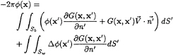
(29)
where:
![]() is the disturbance velocity potential caused by the body,
is the disturbance velocity potential caused by the body,
S is the surface of the body and its vortex (equivalently dipole) wake,
![]() is an onset flow velocity vector,
is an onset flow velocity vector,
x and x′ represent 3-d locations of field and source points, respectively, and all points lie on the body or on the wake,
G is the Rankine source Green function, 1/|x–x′|,
subscript Sb refers to an integral over the body with normal into the body, and
subscript Sw refers to an integral over the wake on which the potential jump from side 1 to side 2 is Δ![]() , and the normal to the wake is in the direction from side 2 to side 1.
, and the normal to the wake is in the direction from side 2 to side 1.
Discretization of the integral equation 29 leads to the set of linear algebraic equations that is the panel method. In formulating it, the jump in velocity potential across any vortex/dipole wake streamline has to be set equal to the jump in velocity potential at the position on the trailing edge of the body from which the streamline originates (c.f. Lee, 1987). Initially, the position of the wake sheet is unknown, and needs to be determined for maximum accuracy. This is done by iteratively solving the integral equation and tracing wake streamlines.
The vortex lattice method, as originally developed by Greeley and Cross-Whiter (1989), is a simplification of the panel method. It requires simpler program input data and provides much faster computation. It's origins actually stem from the lifting body panel method first developed by Hess (1972). That approach was to use both surface source and surface dipole panels, as indicated in equation 29, on lifting surfaces such as aircraft wings and tails, but only source panels on fuselages, which are boat canoe bodies and keel bulbs here. To properly model the circulation at the lifting surface roots it was carried into the fuselage to the centerline. If the sum of the body-entering circulations was not zero, the difference was modeled as a centerline vortex that exited the trailing tip of the fuselage.
The simplified vortex lattice method starts with the Hess model, but represents the lifting surfaces as their centerplane distributions of sources and vortex lattices (or, equivalently, dipole panels). In the development of Greeley and Cross-Whiter, hull canoe bodies and keel bulbs have surface source distributions, whereas rudders, keel fins and winglets have centerplane distributions of sources and vortex lattices, with the root circulations of the latter extended into hulls and bulbs as necessary.
Both Greeley and Cross-Whiter (1989) and Ramsey (1996) have done extensive comparisons between the results of panel methods and vortex lattice methods. The only difference in computed forces is that the vortex lattice method gives slightly less lift because the increase in lift slope of a wing due to its thickness is not included in the vortex lattice method. However, the ratio of the induced drag coefficient to the square of the lift coefficient is the same for both methods and that is the quantity which measures the induced drag efficiency of a lift-producing three-dimensional object.
Now, two examples of the use of the vortex lattice code in support of design are given. Figure 15 is a drawing of the submerged portion of an IACC yacht at a heel angle of 20 degrees. It is customary to adjust the fore and aft location of the rig (sails) such that the rudder carries about 20% of the heel force exerted by the sails. This corresponds to rudder angles of about 1 degree in light winds and 3 degrees in strong winds. This amount of rudder loading, sometimes called “pressure”, is common on many kinds of sailing vessels. Since rudders are designed to be underbalanced about their stocks, if there is “helm pressure” the boat turns to windward when the helmsman eases off on his steering force. Sailors
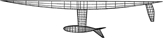
Figure 15: Submerged Portion of an IACC Racing Yacht. It is shown at a heel angle of 20 degrees.
have come to like and expect this behavior. The particular vessel geometry under consideration here is significantly more efficient at generating heel (side) force on the keel fin than on the rudder. Because the keel is not only deeper, but also has winglets, less induced drag occurs when a prescribed side force is generated on the keel than on the rudder. In fact, use of a vortex lattice code has shown that minimum induced drag occurs when the rudder side force is very nearly zero. For typical sailing conditions, the numerical computation predicts the induced drag to be reduced by 8% when the rudder side force is reduced from 20% of the total to zero and the keel side force increased accordingly. Figure 16 shows the time gained vs. wind speed when sailing a 34.4 km windward leeward course due to an 8% reduction in induced drag as determined by a VPP. All of these gains, except for a fraction of a second, occur on the 17.2 km windward portion of the course. These time gains correspond to distance gains of about 7 boat lengths in light wind and 4 boat lengths in strong wind. By top level racing standards, it is substantial. There are further design considerations in this result. In particular, the rudder design needs to be considerably different if the crew learns to sail the boat with minimum rudder force than if the crew chooses a heavily loaded rudder. In the former case, the rudder needs to be as small as possible, even to the extent of requiring dynamic sail trim variations to help steer the boat. The unloaded small rudder simultaneously minimizes the induced drag and the frictional drag of the rudder. On the other hand, if the rudder is heavily loaded there is incentive to make it as deep as possible so as to minimize the extra induced drag. However, to achieve an acceptably low rudder wetted surface with a deep rudder, it must have short chords which leads to small thickness for acceptable thickness fractions. This inevitably results in structural considerations dictating how deep and narrow the rudder can be. It must have sufficient strength and it must be stiff enough to prevent excessive bending, particularly when dynamic wave forces result in substantial time-varying changes in rudder forces.
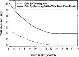
Figure 16: Time Gained when Sailing a 34.4 km to Windward—Leeward Course. Solid line is for moving 20% of the total force off the rudder. Dashed line is for 3 degrees of keel fin twist.
As a second example, the effect of a 3 degree twist of the keel fin is considered. The twist direction has the trailing edge moving to leeward and the leading edge to windward. The twist varies linearly with depth such that it is zero at the root and 3 degrees at the lower tip. Such a twist can be accomplished either by mechanical control or by arranging the center of gravity of the ballast bulb aft of the structural shear center of the keel fin. The reason why such a twist may be beneficial is that for a keel configuration with winglets as shown, the vertical circulation distribution on the fin for minimum induced drag is nearly uniform. However, a structurally sound keel fin can be substantially smaller at the tip (bottom) than at the root (top) since the bending moment with the boat heeled is much smaller at the bottom. Making the keel small at the bottom, to the extent permitted by structural considerations, minimizes the friction drag due to reduced wetted surface, but increases the induced drag unless some other means is used
to increase circulation at the bottom. Twist accomplishes this.
Use of a vortex lattice computer code has shown that the twisted configuration has 96% of the induced drag of the untwisted configuration. The reduction in time to sail the 34.4 km course with this reduction in induced drag is shown in Figure 16.
6.5
Added Resistance Due to Sea Waves
Speed reduction of ships by sea waves from ahead is hydrodynamically very complicated, involving all the nonlinearities related to breaking waves, ship slamming, large relative motions between the ship and the water, and more. The present state-of-the-art for applying numerical hydrodynamics to this problem does not account for these large motion and wave breaking effects. Rather, the numerical method for added resistance is at the lowest contributing order in wave amplitude. This is order two with the added resistance due to a wave being proportional to the square of its amplitude. The approach used is to determine the added resistance for sinusoidal waves individually and to combine the contributions from all the waves. In spite of the low order of the numerical approximation, it provides helpful results which must be included in the total resistance for predicted boat speeds to be in reasonable correspondence with actual sailing speeds. Although the detailed accuracy is not as good as we would like, the difficulty and high cost of meaningful added resistance experiments more or less forces one to take the numerical approach and do it as well as possible.
The added resistance operator, A(ω,ψ) is the ratio of the added resistance to the square of the amplitude of a wave of circular frequency ω and angle ψ. ψ is 0 for stern seas and 180 degrees for head seas. For a long crested (two-dimensional) sea approximation, the mean added resistance, Dw for a sea wave spectrum S(ω) with wave angle ψ is:
(30)
The role of numerical hydrodynamics is the determination of A(ω,ψ). Until quite recently, the procedure of Gerritsma and Beukelman (1972) gave the best agreement between computation and experiment. This procedure uses “strip theory” to estimate the added resistance from the rate of energy imparted to radiated waves caused by relative vertical motions between the ship and the water. Part of
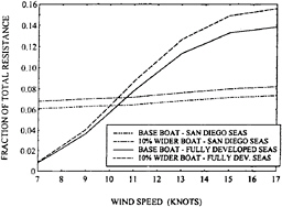
Figure 17: Added Resistances of two IACC Designs in Two Sets of Sea Conditions.
the contribution to added resistance from sea wave diffraction by the ship is neglected in the procedure.
Recent advances have led to the calculation of the added resistance with panel methods, as exemplified in the works of Sclavounos and Nakos (1993) and Sclavounos (1995). As in the aforementioned wave resistance computations by the same people, the linearized free surface problem about the double body basis flow is determined. This is a more accurate approach than earlier procedures and provides a more representative treatment of the effects of diffracted waves. It is, however, still limited to the second order effects. Sclavounos has reported (private communication) that theoretical results were brought into improved agreement with model scale measurements when the vessel length was “stretched” to the wetted length associated with the steady flow.
Figure 17 shows the added resistance computed by the panel methods and equation 30 for two IACC yachts. One is a “base boat” and the other has the waterline beams increased by 10% and the canoe body depth decreased by 10% so as to maintain displacement. This pair of shapes is chosen for demonstration here because for fixed displacement and length, beam is the dominant parameter for variations in numerically-determined added resistance. In the figure, the added resistance is shown as a fraction of the total resistance of the base boat sailing to windward as determined through a velocity prediction program.
Computational results are provided in Figure 17 for two sets of wave spectra. The fully developed seas are for Pierson Moskowitz Spectra, SPM, at the indicated wind speeds. The San Diego Seas have spectra SSD which are empirical curve fits to spectra that were measured over the wind speed range in waters
off San Diego, California in 1991. These spectra are given by:
(31)
(32)
where: g is the acceleration of gravity, Uw is the wind speed at a height of 10 meters and the numerical value of the circular frequency ω is used in the last factor of the curve fit equation 32.
Several important conclusions can be drawn from the information in the figure. They are:
-
The added resistance in typical sea conditions is large enough that it must be included in speed prediction procedures if they are to be accurate.
-
Using the correct sea spectrum is important in estimating added resistance. The San Diego spectra differ from fully developed spectra in two ways. First, in light winds the waves are larger than the winds would indicate because waves propagate into the region from other areas. Second, in the heavier winds the seas are generally smaller than fully developed seas because the heavy winds do not last long enough for the seas to become fully developed.
-
Except for the fully developed seas in heavier winds, the difference in computed added resistance is less than observed performance differences in disparate designs. Experience shows that the wider boat suffers in waves by considerably more than the 1% of total resistance indicated in the figure. The author believes this disagreement is mainly due to lack of incorporation of nonlinear effects in present numerical methods.
6.6
Mean Forward Thrust Due to Unsteady Motions
An intriguing subject is the potential for dynamic thrust, which is a mean forward thrust due to the flow on appendages associated with unsteady vessel motions and sea waves. On traditional vessels this thrust is very small, and therefore it has not received much attention in the history of sailing vessel hydrodynamics. However, the dynamic thrust can be larger on the nearly horizontal keel and rudder
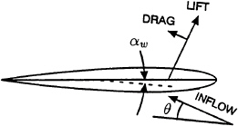
Figure 18: Forces on a Wing Section at an angle of Attack.
winglets which have been used recently on some vessels. Before explaining a mathematical method for relating dynamic thrust to design parameters, a general description of its origins is provided.
As is sketched in Figure 18, the lift on an air or hydrofoil is perpendicular to the incident flow and the drag is parallel to it. For explanatory purposes here, foils with symmetrical thickness forms are considered. Lift occurs when the inflow has an angle of attack, αw+θ, with respect to the nose-tail line of the foil and a component of this lift force is forward when αw≠0. The inflow angle of attack on horizontal appendages occurs when there is a relative vertical velocity due to vessel motions or vertical components of the “orbital velocities” of the sea waves. As shown in the figure, there is a net forward force if Lift×sin(|αw|)>Drag×cos(αw). Importantly, this net forward force occurs if αw is either positive or negative. As the vessel undergoes unsteady motions in waves, the inflow angle to a horizontal appendage oscillates between upward and downward. The lift vector direction can be mainly up or down, but it almost always has a forward component. If the average of this forward component exceeds the average of the aft component of the drag, positive average thrust occurs. Otherwise, there is net drag.
The dynamic thrust can be quantitatively estimated by the use of lifting line theory, largely because horizontal appendages that are efficient at its generation necessarily have large aspect ratios. For relative motions of frequency fe with boat speed Vb and appendage dimensions of order ℓ, the thrust-producing effects have reduced frequencies, feℓ/Vb, which are low enough for quasi-steady lifting line or lifting surface theory to be accurate. Ship hydrodynamicists came to this conclusion on the general bases of unsteady hydrodynamics and dimensional analysis over six years ago, and more recently Dr. Spiros Kinnas (private communication) has shown this to be the
case in a computation using fully unsteady lifting surface theory. The quasi-steady lifting line analysis is used here.
In this approximate analysis, the yaw motions of the vessel are neglected since they are strongly influenced, and often minimized, by the way the vessel is steered. In addition, the dynamic thrust on generally vertical appendages, such as a keel fin or a rudder are not considered. Just the dynamic thrust on horizontal appendages such as a rudder wing or keel winglets is analyzed. The effects of spanwise flow are neglected.
The relative angle of incidence on the wing is αw+θ cos φ, where θ is the pitch angle of the boat and φ is the, presumed steady, heel angle. The lift coefficient, CL, is given by:
CL=2πκ(αw+θ cos φ) (33)
Ignoring a small increase due to thickness of the wing, the lift slope factor, κ (c.f. Glauert, 1959 and Thwaites, 1960), is given by:
(34)
where RA is the aspect ratio and χ is the sweep angle of the wing.
Using the approximation of an elliptical spanwise circulation distribution, the induced drag coefficient, ![]() is:
is:
(35)
Thus, the forward thrust, T, to lowest order in αw and temporarily neglecting viscous effects, is:
(36)
where Ap is the planform area of the wing and β≡4/RA.
The angle of incidence, to lowest order, is given by:
(37)
where w is the relative vertical velocity at the fore and aft location of the wing. It is the difference between the vertical component of the sea wave orbital velocity and the heave velocity of the boat at the wing location. Since the boat is both heaving and pitching, w depends not only on time, but also on the fore and aft location of the wing. Denoting statistical (or time) averages by overbars, taking the average of equation 36 and using equation 37 provides the fundamental equation for the dynamic thrust, Td.
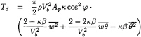
(38)
The ship motions are approximated as being linearly dependent on the sea state with complex transfer functions (frequency responses) from sea wave elevation to heave of Hζw(ωe) and to pitch of Hζθ(ωe). In practice, these transfer functions are determined numerically from strip theory (c.f. Salvesen et al., 1970)) or from a panel method (c.f. Nakos and Sclavounos, 1990). Then, for a one sided sea wave encounter frequency spectrum S(ωe):
(39)
(40)
(41)
Equation 38 is the fundamental equation for dynamic thrust and can be used when the viscous and parasitic drag of the thrust-producing wing are accounted for in the appendage friction drag. This procedure is appropriate for performance prediction of a design with keel winglets whose principal purpose is reduction of induced drag, but which can also produce dynamic thrust.
For force comparisons of various designs of wings whose principal purpose is to generate dynamic thrust, or to decide whether to use such a wing at all, it is useful to consider the difference of the dynamic thrust and the friction and parasitic drags of the wing.
Here, an example is provided for a rudder wing located at a depth of 3 meters and 8 meters aft of midship on an IACC yacht. The wing area is 1 square meter. It has an aspect ratio of 9, a taper ratio (tip chord/root chord) of 1/2 and a sweep angle of 25 degrees. The wing has an NACA 0012 section and its friction drag coefficient is approximated from XFOIL (Drela, 1989) results at a Reynolds number of 1.5 million as 0.008+0.164 α2, where the relative angle of incidence, α, has units of radians. The angle of incidence used in the friction drag calculation is the rms relative incidence angle which is determined
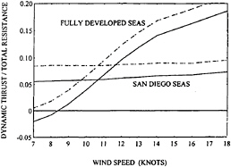
Figure 19: Dynamic Thrust from a Rudder Wing for Windward Sailing. The dynamic thrusts are shown by dashed lines and the dynamic thrusts minus the friction and interference drags are shown by solid lines.
in terms of the quantities used in this section as:
(42)
The interference drag area, AI, between the wing and the rudder is taken as that given by Hoerner (1965) for strut junctions:
(43)
where t is the thickness and c is the chord length at the root intersection.
Figure 19 shows both the dynamic thrust and the difference between the dynamic thrust and the sum of the friction and interference drags for upwind sailing in fully developed seas with spectra given by equation 31, and for San Diego seas with spectra given by equation 32. The angle between the seas and the course of the boat is taken as 142 degrees (38 degrees from ahead) for the calculations.
The dynamic thrust is greatly diminished by reducing the wing aspect ratio. Figure 20 shows the dynamic thrust less the friction and interference drags in fully developed seas for a wind speed of 9 knots, both upwind and downwind, as functions of aspect ratio. All other quantities are the same as in the preceding example except the taper ratios are 2/3 and the wave angle for the downwind case is taken as 30 degrees from astern.
Findings from numerical studies of a broad range of wing parameters include:
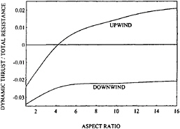
Figure 20: Dynamic Thrusts, Upwind and Downwind, in Fully Developed Seas for a Wind Speed of 9 Knots as Functions of Wing Aspect Ratio.
-
Dynamic thrust, exclusive of friction and interference drag, is positive and significant for upwind sailing, and is generally so small as to be insignificant for downwind sailing.
-
Dynamic thrust less the friction and interference drag of a wing is negative for downwind and upwind sailing in light winds. As the wind strength and the corresponding seas increase, the net thrust becomes positive for upwind sailing in medium winds if the aspect ratio is high, roughly 7 or higher. The net downwind thrust is positive only in strong winds and then of small magnitude.
-
Both the upwind and the downwind net thrusts increase as the wing is moved further aft as a result of the relative phases between heave and pitch. The effect is nearly insignificant for downwind sailing, but can be quite influential for upwind sailing.
The foregoing information refers to numerical calculations according to the method described. Actual sailing experience is somewhat different. In particular, the predicted upwind advantage and the predicted downwind disadvantage of wings are not realized. Rather, the upwind speed gain is generally less than predicted and the downwind speed loss is often much less than predicted. The reasons for this are not well understood at this time. It is an area of interest for further study.
7
Computation of Lift and Induced Drag of Sails
Numerical methods for calculating the lift and induced drag of sails have similarities with the vortex lattice method used for the induced drag and heel force of hull appendage combinations that is described in section 6.4. The essential differences are:
-
The sails are thin, unsymmetrical lifting surfaces. This makes their representation by dipole or vortex sheets complete for the inviscid problem.
-
The inflow speed varies with height in the atmospheric boundary layer. Although the height varying inflow is used in older methods as well as the one used here, all of these methods neglect the influence of spanwise flow on the inflow velocities. Both calculations and measurements show that most of the spanwise flow has speeds that are small in comparison to the inflow speeds so that the error is similarly small due to the mild gradient of the wind speed over most of the sailplan.
The application of lifting surface theory to sails began with the author's work 28 years ago (Milgram, 1968). The sails were represented by vortex lattices and the wakes were flat. The lower boundary beneath the sails was approximated as a flat plane by numerical use of image sails beneath the plane. The plane was at a user-specified location between locations of the water surface and the deck. The procedure was aimed at the design problem for which the pressure distributions were specified and the shapes needed to attain them were computed. For the next 20 years, a number of proprietary programs were developed for the sailmaking industry. It is thought they use the same principles, but also include the analysis problem for which the shapes are specified and the resulting pressure distributions and integrated lift and induced drag forces are computed.
The next significant advancement in the fluid dynamics was the work of Greeley, et al. (1989). They solved the analysis problem iteratively with the vortex wakes of the sails convected along the horizontal components of streamlines at each step. In addition, the sails and their images were heeled with respect to the image plane. The resulting computer program has been broadly used to evaluate lift and induced drag of sail shapes.
Optimized sail design requires use of both design and analysis programs. When the sails are a mainsail and
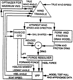
Figure 21: Method of Evaluation of Sail Shape on Performance.
a jib which does not go the full height of the mainsail, computed shapes for ideal pressure distributions are ones which cannot be built. The induced flow on the mainsail due to the jib and its wake is to windward below the top of the jib and to leeward above it. The shape of a mainsail that can accommodate this jib-induced flow variation and also have an ideal pressure distribution is generally complex and connot be achieved with sail fabric that cannot support compression. Hence, results of the design programs can be used to guide the shapes of sails, but generally their designed shapes cannot be attained exactly. The analysis program can then be used to evaluate lift and induced drag on “the designer's approaches” toward the ideal shapes.
The best use of an inviscid sail analysis program is for comparing performance of candidate designs. In order to do that, the form and friction drag of the sails must be included and the resulting total sail forces used in a VPP. For windward sailing, which is the condition for which the process is most useful, the operational true wind angle, ψ, must be optimized in the VPP such that the speed made good to windward, VMG=Vb cos ψ, is maximized. Since the sail forces depend on ψ, or more precisely on the apparent wind angle, the process is necessarily iterative. Figure 21 is a block diagram of this process as developed by Mr. Jack Kleene and the author and which has been found to be effective in practice.
Ramsey (1996) has taken the next step in development of numerical hydrodynamics of sails: he has added the above water portion of the hull. The sails are represented as vortex lattices with convected wake geometries determined by iteration. The hull can be represented by source panels as in the appendage numerical method of section 6.4, or as vortex quadrilaterals around the periphery of each hull panel. The two methods give total forces within 1% of each other. If a sail is sealed to the deck of the hull, its root circulation is carried on a continuation of the sail through the deck down to the reflection plane. Figure 7 shows the hull, sails and panelization for which we have done computations. The sailing conditions are for a 4.52 m/s wind speed at a height of 10 meters, a boat speed of 4.51 m/s, a heel angle of 20 degrees, and a true wind angle of 40 degrees from ahead. The true wind velocity has a logarithmic profile with a roughness height of 0.001 m for heights greater than 0.5 m. Below 0.5 m, where the wind speed is 3.05 m/s, it is reduced linearly to 1.53 m/s at the sea surface. The rapid decrease of the real wind speed with decreasing height to zero at the surface is avoided as it would make the computations singular. The camber and twist distributions are chosen to be consistent with good sails in practice. At the mast, the hull freeboard is 1.3 meters before heeling. For these computations, an image plane is located at the water surface. Computations have been carried out for the sails without a hull, for the sails and the hull together with spaces between the bottoms of the sails and the deck, and for the sails and hull with the bottom of the jib sealed to the deck. Table 1 shows the results for the forward and side forces. Computed results for the effect of the hull on the total forces, which include aerodynamic pressures on the hull, are new and of particular interest. The existence of the hull adds significantly to the forces, particularly on the jib which is closest to it, and improves (decreases) the ratio of induced drag coefficient to the square of the lift coefficient. This is particularly true when the bottom of the jib is sealed to the deck. Figure 23 shows the vertical circulation distributions on the sails for each of these cases. It demonstrates the influence on the mainsail of the jib which is of lesser span.
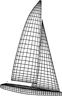
Figure 22: Geometry and Panelization for Example Sail Computations. The view shown is from the leeward side with the boat heeled 20 degrees, with the viewpoint elevated and forward of the midship.
Table 1: Sail Forces. Units are Newtons.
|
NO HULL |
HULL NO JIB SEAL |
HULL WITH JIB SEAL |
|
|
FORWARD FORCE |
|||
|
HULL |
58 |
85 |
|
|
JIB |
2376 |
2505 |
3083 |
|
MAIN |
1544 |
1571 |
1588 |
|
TOTAL |
3920 |
4133 |
4756 |
|
HEEL FORCE |
|||
|
HULL |
516 |
525 |
|
|
JIB |
6901 |
7212 |
8173 |
|
MAIN |
8529 |
8600 |
8614 |
|
TOTAL |
15430 |
16329 |
17312 |
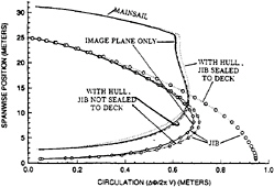
Figure 23: Circulation Distributions on the Sails
References
[1] M.Drela. Xfoil: An analysis and design system for low reynolds number airfoils . In Lecture Notes in Engineering, volume 54, Low Reynolds Number Aerodynamics. Springer-Verlag, New York, 1989.
[2] M.Drela and M.B.Giles. Viscous-inviscid analysis of transonic and low reynolds number airfoils . AIAA Journal, 25(10), October 1987.
[3] R.Eppler and D.Somers. A computer program for the design and analysis of low speed airfoils . Technical Memorandum TM-81862, NASA, 1980.
[4] S.E.Euerle and Greeley D.S. Towards a rational upwind sail force model for vpps. In Proceedings of Eleventh Chesapeake Sailing Symposium. Society of Naval Architects and Marine Engineers, 1993.
[5] J.Gerritsma and W.Beulelman. Analysis of the resistance increase in waves of a fast cargo ship . International Shipbuilding Progress, 19, 1972.
[6] H.Glauert. Airfoil and Airscrew Theory. Cambridge University Press, London, 1959.
[7] D.S.Greeley and J.H.Cross-Whiter. Design and performance of sailboat keels. Marine Technology, 26(4):260–281, 1989.
[8] D.S.Greeley, K.L.Kirkman, A.L.Drew, and J.H.Cross-Whiter. Scientific sail shape design. In Proceedings of Ninth Chesapeake Sailing Symposium. Society of Naval Architects and Marine Engineers, 1989.
[9] J.L.Hess. Calculation of potential flow about arbitrary three-dimensional lifting bodies. Technical Report MDC J5679–01, Douglass Aircraft Company, 1972.
[10] S.F.Hoerner. Fluid Dynamic Drag. S.F.Hoerner, Midland Park, New Jersey, 1965.
[11] K.L.Kirkman and D.R.Pedrick. Scale effects in sailing yacht hydrodynamic testing. Transactions of the Society of Naval Architects and Marine Engineers, 1974.
[12] G.C.Lauchle and G.B.Gurney. Laminar boundary-layer transition on a heated underwater body. Journal of Fluid Mechanics, 144:79– 101, 1984.
[13] J.T.Lee. A Potential Based Panel Method For the Analysis of Marine Propellers. PhD thesis, Department of Ocean Engineering, Massachusetts Institute of Technology , Cambridge, MA 02139, 1987.
[14] L.M.Mack. Transition prediction and linear stability theory. In Laminar-Turbulent Transition, pages 1–1—1–22, 1977. AGARD-CP-224.
[15] J.H.Michell. The wave resistance of a ship. Philosophical Magazine, pages 106–123, 1898.
[16] W.Milewski. Coupled Potential Flow and Boundary Layer Equations for Three Dimensional Objects . PhD thesis, Department of Ocean Engineering, Massachusetts Institute of Technology , Cambridge, MA 02139, 1996. In Preparation.
[17] J.H.Milgram. Section data for thin, highly cambered airfoils in incompressible flow. Contractor Report CR-1767, NASA, 1971.
[18] J.H.Milgram. Naval archicture technology used in winning the 1992 america's cup match. Transactions of the Society of Naval Architects and Marine Engineers, 101:399–436, 1993.
[19] J.H.Milgram. The aerodynamics of sails. In Proceedings of 7'th Symposium on Naval Hydrodynamics. Office of Naval Research, 1968. Held in Rome, Italy.
[20] J.H.Milgram. The analytical design of yacht sails. Transactions of the Society of Naval Architects and Marine Engineers, 1968.
[21] D.E.Nakos, D.Kring, and P.D.Sclavounos. Rankine panel methods for transient free surface flows. In Proceedings, Sixth International
Conference on Numerical Ship Hydrodynamics. University of Iowa, 1993.
[22] D.E.Nakos and P.D.Sclavounos. Ship motions by a three dimensional rankine panel method. In Proceedings of 18'th Symposium on Naval Hydrodynamics. Office of Naval Research, 1990. Held at University of Michigan, Ann Arbor, August 20–23, 1990.
[23] C.W.Prohaska. A simple method for the evaluation of the form factor and the low speed wave resistance. In Proceedings of 11'th ITTC. International Towing Tank Conference, 1966.
[24] W.Ramsey. Numerical Methods for Flows Around Lifting Bodies with Vortex Wake Rollup. PhD thesis, Department of Ocean Engineering, Massachusetts Institute of Technology , Cambridge, MA 02139, 1996. In Preparation.
[25] B.S.Rosen, J.P.Laiosa, W.H.Davis, and D.Stavetski. Splash free-surface code methodology for hydrodynamic design and analysis of iacc yachts. In Proceedings of Eleventh Chesapeake Sailing Symposium. Society of Naval Architects and Marine Engineers, 1993.
[26] N.Salvesen, E.O.Tuck, and O.Faltinsen. Ship motions and sea loads. Transactions of the Society of Naval Architects and Marine Engineers, 78, 1970.
[27] P.D.Sclavounos. A practical computer method for solving ship-wave problems. In Proceedings, Second International Conference on Numerical Ship Hydrodynamics. University of California at Berkeley, September 1977.
[28] P.D.Sclavounos. Computation of Ship Wave Interactions, chapter 4, pages 177–231. Computational Mechanics Publications, 1995.
[29] P.D.Sclavounos and Nakos D.E.Seakeeping and added resistance of iacc yachts by a three-dimensional panel method. In Proceedings of Eleventh Chesapeake Sailing Symposium. Society of Naval Architects and Marine Engineers, 1993.
[30] B.Thwaites. Incompressible Aerodynamics. Oxford University Press, Oxford, 1960.
[31] E.O.Tuck. The Steady Motion of a Slender Ship. PhD thesis, University of Cambridge, Cambridge, England, 1963.
[32] P.Van Oossanen. Predicting the speed of sailing yachts. Transactions of the Society of Naval Architects and Marine Engineers, 101:339–397, 1993.
Acknowledgements
The author is appreciative of the technical information provided by America3 Foundation (A3) and by the Partnership for America's Cup Technologies (PACT). It has made this a more informative paper than would otherwise be the case. Five organizations which engaged in extensive technical efforts in support of their designs of IACC yachts were contacted and only A3 and PACT provided information and permission to use it. This is why much of the technical information provided herein is attributed to people associated with these organizations.
Hydrodynamics in Advanced Sailing Vessel Design
Errata
Equation (18) contains a typographical error. The corrected equation is:
(18)
Equation (24) contains a typographical error. The corrected equation is:
(24)
The rightmost data point in Figure 12 is in error. The corrected figure follows:
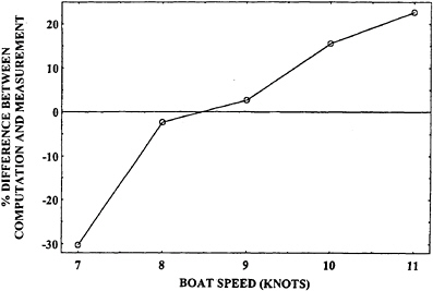
Figure 12: Error in the Wave Making Resistance of an IACC Yacht Computed by Sclavounos.
The labeling and orientation in Figure 18 are not correct. The corrected figure follows:
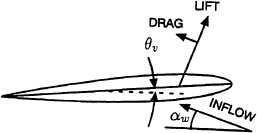
Figure 18: Forces on a wing section at an angle of attack.
In the second paragraph below the figure change αw+θ to αw+θv.


