
Computations of Wave Loads Using a B-Spline Panel Method
C.-H.Lee, H.Maniar, J.Newman, X.Zhu (Massachusetts Institute of Technology, USA)
Abstract
This paper describes the development of a higher-order panel method based on B-splines, and its application to problems involving linear and nonlinear wave interactions with floating or submerged bodies. The use of B-splines permits a very accurate representation of the body geometry, and a continuous representation of the velocity potential on the body surface. These features result in more efficient and robust solutions relative to the conventional low-order panel method.
Several applications are described to illustrate the computational advantages of this method. These include first-order solutions for a floating hemisphere, a tension-leg platform, and a long periodic array which is representative of very large platforms proposed for floating airports and cities. Also considered are second- and third-order wave loads, where fundamental difficulties exist in evaluating the free-surface forcing functions using the low-order method. This is particularly important at third order, where we present preliminary results from an investigation aimed at predicting the occurrence of ringing.
1.
Introduction
Computations based on panel methods have achieved widespread use among practicing engineers and hydrodynamicists for external-flow potential problems. In applications concerning the wave loads and motions of offshore platforms, and other stationary vessels, the first-order analysis in the frequency domain is now routine (Korsmeyer et al. [10], Herfjord & Nielsen [6]). Panel methods can be used not only for single bodies but also for multiple interacting vessels, with important applications to marine operations. Success also has been achieved in extending this method to the analysis of second-order wave effects (Molin & Chen [18]; Eatock Taylor & Chau [3]; Lee & Newman [12]). However, notwithstanding the popularity and success of this technique, there are various special problems where the computational burden is severe, or where quantities are required such as gradients of the velocity field, which cannot be computed robustly from the conventional ‘low-order' panel method.
In low-order methods the submerged surface of the body is represented by a large number N of flat quadrilateral panels, and the velocity potential (or the source strength) is assumed piecewise constant on each panel. Only sources were used in the pioneering work of Hess & Smith [7], with the unknown source strength determined from an integral equation derived from the boundary condition on the body. In the complementary procedure where sources and normal dipoles are used, the potential is determined more directly from an integral equation based on Green 's theorem. In either of these approaches, the integral equation is replaced by a system of linear equations, with the number of unknowns equal to N.
The use of flat panels simplifies the evaluation of the integrated singularity distribution on each panel, but a relatively large number of panels are required to achieve accurate representations of the geometry and the potential. A more fundamental restriction is that the potential derived from Green's theorem cannot be differentiated analytically to derive the fluid velocity on or near the body surface; this difficulty can be circumvented in a limited manner by using a distribution of sources only, but that method also fails if gradients of the velocity field are required.
Higher-order panel methods have been devel-
oped to overcome these difficulties. Most of the higher-order methods are based on piecewise polynomial approximations of the geometry and potential on each panel, usually restricted to linear or quadratic representations using local polynomials of first- or second-degree, respectively. In this paper we describe a different higher-order approach, where B-spline basis functions are used to represent the geometry and potential. This offers the possibility of a more continuous representation, with greater geometrical flexibility and numerical efficiency. Following a preliminary investigation of this technique in two dimensions (Hsin et al., [8]), we have developed a three-dimensional panel program which will be referred to as ‘HIPAN'. A more detailed description of the method is contained in the thesis of Maniar [16].
HIPAN was developed initially to solve linearized radiation-diffraction problems in the frequency domain. Thus the body is fixed, or performing small oscillatory motions about a fixed mean position, and plane progressive waves are incident from a prescribed direction. The fluid is either of constant finite depth, or infinitely deep. The body may be floating on the surface or submerged. For this case the free-surface Green function can be used effectively. The analogous low-order panel method WAMIT, which is described by Lee [11], can be used to test the accuracy and relative computational efficiency of HIPAN. The efficiency of HIPAN is most apparent for relatively complicated body shapes. This will be illustrated by considering a large array of floating cylinders similar to a floating bridge. In that particular problem we find not only that substantially larger arrays can be analyzed, but also that the results display very interesting features closely related to the occurrence of trapped waves in a channel.
In many applications important nonlinear effects must be analyzed, particularly the second-order sum- and difference-frequency loads which occur at relatively high and low frequencies compared to the first-order wave spectrum. High-frequency loads are important in cases where resonant structural response is encountered. Examples include hull deflections of long slender ships, bending of vertical monotowers, and vertical motions of tension-leg platforms. Conversely, low-frequency loads are important for rigid-body motions where the restoring forces are relatively weak. Examples include the horizontal oscillations of moored and towed vessels, and the vertical response of vessels with small waterplane areas. The analysis of these second-order loads can be performed using a low-order panel method, but the computational burden is quite large and much care is necessary to ensure robust results. The extension of HIPAN to include second-order loads is currently in progress, and we are not able to show complete computations, but preliminary results which have been obtained demonstrate the improvements that may be achieved using the B-spline methodology in the second-order analysis.
It should be noted that we refer to ‘order' in two completely different contexts here, one specifying the numerical approximation of the geometry and velocity potential on the body surface, and the other referring to the order of the perturbation expansion in terms of the amplitude of the waves and body motions. Low-order and higher-order panel methods are distinguished by the type of numerical approximations used, whereas first-and higher-order wave loads are defined with respect to the corresponding powers of the wave amplitude.
Recent attention in the offshore community has been directed toward higher-order nonlinear loads which are thought to cause ‘ringing', a hydrodynamic/structural resonance which has been observed for large platforms in extreme wave conditions. The relevant frequencies suggest that ringing may be caused by third-harmonic wave loads, and this has motivated two recent studies which are restricted to the simplest possible geometrical configuration, a vertical circular cylinder. In the work of Faltinsen et al. [4] a perturbation scheme is employed appropriate to the regime where the cylinder radius and wave amplitude are of comparable magnitude, and both are small compared to the wavelength. In the complementary work of Malenica & Molin [15], a conventional Stokes expansion is used with the wave amplitude assumed small compared to the cylinder radius and wavelength and without restricting the radius/wavelength ratio. Partly to clarify the differences between these two works, and also to develop a more general computational tool for analyzing practical bodies, we have extended HIPAN to include third-order loads. Here too our present results are incomplete, but they do indicate that the Stokes expansion may be more appropriate for contemporary platforms.
In Sections 2–3 we review the boundary-value problems to be addressed, and the formulation of the panel method for solving these problems based on B-splines. Solutions of several illus-
trative problems are described in Section 4. In the concluding Section 5 other possible applications and extensions of HIPAN are discussed. For simplicity we restrict our attention to diffraction problems where the body is fixed. Except where noted the fluid depth is assumed infinite.
2.
The Boundary-Value Problem
Cartesian coordinates x=(x, y, z) are defined with z=0 the plane of the undisturbed free surface and z<0 the fluid domain. In accordance with the assumptions of potential theory, and a perturbation solution in terms of a small parameter ![]() (e.g. the incident-wave slope), the velocity potential is expanded in the form
(e.g. the incident-wave slope), the velocity potential is expanded in the form
(1)
where t denotes time.
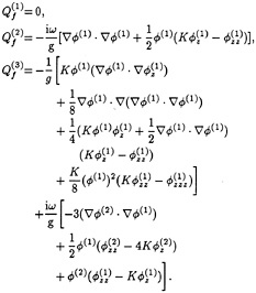
Assuming a discrete spectrum with frequency components ωn, the first-order potential can be expressed as
(2)
where ωn>0. The second- and third-order potentials, which result from quadratic and cubic interactions among first-order solutions, can be expressed as
(3)
(4)
where Re denotes the real part of the complex quantity.
The complete higher-order solutions contain a variety of frequency components. For example, the second-order solution contains the second-harmonic, mean and sum- and difference-frequency components. The third-order solution contains more diverse combinations of frequency components. To simplify the discussion here we consider the case of monochromatic first-order incident waves. Specifically we consider the second-harmonic and mean components of the second-order solution and the third-harmonic component of the third-order solution.
The diffraction potentials can be decomposed into incident and scattering components. In general, it is convenient to solve for these potentials separately, due to their different asymptotic behavior at the far-field. However in the case of monochromatic incident waves in infinite water depth, the second- and third-order incident wave potentials vanish and it is not necessary to distinguish between the diffraction and scattering components at these orders.
The diffraction potentials are subject to the free-surface condition
(5)
where j=1, 2, 3. The forcing functions at each order j are evaluated from the following equations, with z=0:
(6)
Each of the diffraction potentials also satisfies the condition of zero normal velocity on the body surface, and vanishes at large depths. In addition, they are subject to appropriate radiation conditions in the far-field. The scattering part of the first-order potential satisfies a Sommerfeld radiation condition. The far-field behavior of the second- and third-order potentials include outgoing ‘free' waves, which satisfy a Sommerfeld radiation condition, and ‘locked' waves which are in phase with the ![]() [15].
[15].
Integral equations suitable for evaluating the diffraction potentials are derived by applying Green's theorem to the volume of fluid in the domain which is bounded by Sb, Sf, and a closure surface which is in the far field and at large depths below the free surface. For this purpose we use
the wave source potential as the Green function (cf. [19], equation 7.9). The resulting equations are Fredholm integral equations for the unknown ![]() (j) over the domain Sb. The first-order diffraction potential is obtained from
(j) over the domain Sb. The first-order diffraction potential is obtained from
(7)
and the higher-order potentials from
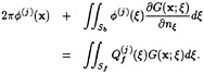
(8)
In the forcing function on the right-hand-side of the latter equation the integrals over Sb and the far-field closure vanish due to the boundary conditions of the diffraction potentials as stated above.
The principal difficulty in the computation of the higher-order potentials lies on the evaluation of the integral over the free surface. The integrands are oscillatory, and slowly decaying. Truncation at a finite distance from the body is generally not adequate. Instead, following Lee & Newman [12], Sf is divided into two regions separated by a circle which encloses the body, and is of sufficiently large radius so that the effect of the evanescent modes of the scattering waves is negligible outside the circle, compared to the propagating modes. In this infinite outer region, the Green function and the velocity potentials can be expanded in Fourier-Bessel series and the integrals can be reduced to the sums of one-dimensional integrals of the products of the corresponding Bessel functions. The latter integrals are nontrivial, but they can be evaluated numerically with appropriate algorithms. Direct numerical quadrature is used for the evaluation of the surface integral over the finite inner region. The details of this procedure, and the utilization of B-spline basis functions are discussed in Section 3.3.
The integrated wave loads or exciting forces are evaluated by integrating the pressure due to the diffraction potentials over the wetted surface of the body. The final expressions for the first-, second- and third-order forces are
(9)
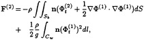
(10)
and
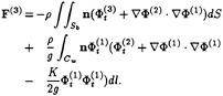
(11)
Here ρ is the water density, Cw denotes the intersection of the body with the mean free surface, and n is the normal vector to the body surface. For the corresponding moments n is replaced by (x×n).
3.
The B-spline Methodology
We consider a three-dimensional body (or ensemble of separate bodies) where the submerged body surface consists of a finite set (p=1,…, ![]() ) of continuous surfaces, referred to as patches. The Cartesian points x=(x, y, z) on each patch are mapped to a rectangular parametric domain (u, v) by a continuous mapping function, which is assumed here to be described by a B-spline tensor product expansion of the form
) of continuous surfaces, referred to as patches. The Cartesian points x=(x, y, z) on each patch are mapped to a rectangular parametric domain (u, v) by a continuous mapping function, which is assumed here to be described by a B-spline tensor product expansion of the form
(12)
Here ![]() and
and ![]() are B-splines of order
are B-splines of order ![]() (degree
(degree ![]() −9) in the parametric variables u and v respectively, and
−9) in the parametric variables u and v respectively, and ![]() are prescribed vertices or coefficients. The total number of
are prescribed vertices or coefficients. The total number of ![]() p and
p and ![]() splines used for the approximation are
splines used for the approximation are ![]() p and
p and ![]() p respectively.
p respectively.
For a detailed description of B-splines we refer to DeBoor [2]. It suffices here to note that B-splines are polynomial functions which are nonzero over a finite span (support), and that their shape and continuity are dependent on the order and on a monotonic increasing sequence of real numbers

(13)
which are called knots. The rectangular parametric space which is mapped by (12) onto the physical surface is
(14)
This is referred to as the usable space.
As an example, Figure 1 shows one quadrant of a tension-leg platform (TLP), represented by 35 patches. On the pontoons a total of 32 patches are used, and outlined separately in the figure. Three larger patches are used to represent the column, including one on the bottom circular disk, one on the side to represent the complete circular cylinder above the pontoons, and one on the lower outside surface of the cylinder between the pontoons. (While not relevant to the representation of the geometry, each of these larger patches is subdivided for hydrodynamic purposes into smaller panels which we define later. These panels are outlined in Figure 1.)
Utilizing the parametric space provided by each patch, we also approximate the potential by a B-spline tensor product expansion. Thus, the potential on patch p is represented in the form
(15)
Here ![]() and
and ![]() are B-splines of order k in the same parametric variables u and v, dependent on the knot vectors
are B-splines of order k in the same parametric variables u and v, dependent on the knot vectors
(16)
and ![]() are unknown complex coefficients to be solved for.
are unknown complex coefficients to be solved for.
Since different B-splines may be used in (12) and (15) the method is not restricted to be isoparametric. To ensure that the usable parametric space implicit in (15) matches that of the geometry (12), we require that ![]()
![]() Multiple knots may be used in (12–13) to represent special features of the patch geometry. Multiple knots are not allowed in the usable space for the potential splines. In the absence of multiple knots for potential splines, we define Mp=Ip–k+1 and Np=Jp–k+1, which correspond to the total number of non-zero intervals between consecutive knots of the usable space in the u and v directions respectively.
Multiple knots may be used in (12–13) to represent special features of the patch geometry. Multiple knots are not allowed in the usable space for the potential splines. In the absence of multiple knots for potential splines, we define Mp=Ip–k+1 and Np=Jp–k+1, which correspond to the total number of non-zero intervals between consecutive knots of the usable space in the u and v directions respectively.
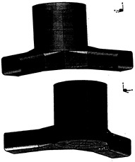
Figure 1: One quadrant of a TLP described by 35 B-spline patches. The lines on the surface are panel boundaries.
3.1
Features of the method
By allowing piecewise continuous bodies to be described in a patchwise fashion, one can represent a wide variety of complex structures with a very accurate geometric description of each patch.
While the potential is approximated in the same parametric variables as the surface, these two representations are otherwise independent. Consequently, increasingly accurate potential approximations can be sought without reconstructing the geometry.
The representations (12) and (15) are local approximants due to the finite support of the splines. Further, implicit in these equations is the possibility of a nonuniform distribution of the splines over the parametric space. Both of these features are desirable for approximating the solution in the vicinity of flow singularities (e.g., in the vicinity of body edges and the free surface).
An approximant based on B-splines of order k has (k–2) degrees of continuity everywhere on a patch, unlike many higher-order methods where continuity is ensured only over a panel or element. Continuous descriptions of parametric derivatives of the potential can be obtained simply by analytic differentiation. Cartesian derivatives of the potential can also be derived analytically, using the parametric derivatives of the patch geometric description (see Bingham & Maniar [1]). Not only first- but also higher-order derivatives of the
potential can be derived, provided the order of the B-splines is appropriately selected.
No explicit conditions are imposed on the potential at the common boundaries of the patches. This absence of ‘connectivity' between patches greatly simplifies the implementation of the method. No special considerations are required if a patch boundary coincides with a surface discontinuity where the potential is singular, as in the case of the corner at the lower edge of the TLP column in Figure 1.
3.2
The integral equation
The unknown coefficients which appear in (15) may be determined by imposing Green's theorem (7–8). For the sake of generality we define the forcing function which appears on the right side of this equation by ![]() , and also the residual r, by
, and also the residual r, by
(17)
i.e., the difference between the left- and right-hand sides of the integral equation. To obtain a linear system of equations for the complex coefficients, ![]() a Galerkin procedure is adopted. Specifically, we minimize the residual with respect to each of the (potential) B-spline tensor products directly over their support
a Galerkin procedure is adopted. Specifically, we minimize the residual with respect to each of the (potential) B-spline tensor products directly over their support ![]() in the usable parametric space. Thus,
in the usable parametric space. Thus,
(18)
for i=1, 2, …, Ip; j=1, 2, …, Jp; p= 1, 2, …, ![]() . Each patch provides the same number of equations as the number of unknowns, resulting in a square complex dense system of equations of dimension U×U where
. Each patch provides the same number of equations as the number of unknowns, resulting in a square complex dense system of equations of dimension U×U where
(19)
As a result of the Galerkin procedure, the influence coefficients in the linear system are double spatial integrals of ∂G/∂n. These coefficients are evaluated by a semi-discrete Galerkin approach where the outer integral in (18) is replaced by a fixed order (Ng) product Gauss rule, applied to each of the intervals between the knots ![]() of the support of the (potential) splines in usable space. For this purpose Gauss-Legendre quadratures are efficient, and numerical experiments indicate that Ng=2 and 3 suffice for linear and cubic B-splines, respectively. With this algorithm, the field points of the Green function in the inner integration are specified by the Gauss nodes in parametric space.
of the support of the (potential) splines in usable space. For this purpose Gauss-Legendre quadratures are efficient, and numerical experiments indicate that Ng=2 and 3 suffice for linear and cubic B-splines, respectively. With this algorithm, the field points of the Green function in the inner integration are specified by the Gauss nodes in parametric space.
Special attention is required for the inner integrals, to account for the Rankine singularity of the Green function. When the field point lies within the domain of integration, the singularity is analytically removed and the resulting integrand expanded in a series with algebraic terms which are integrable in closed form. For other cases, and for the integrals of the non-singular part of the Green function, Gauss-Legendre quadratures are used. If the field point is near the integration domain, adaptive subdivision is used for the nearly-singular Rankine component to preserve the accuracy of the quadrature scheme. The contribution to the Green function from the free surface is evaluated using the algorithms described by Newman [19]. For further details see Maniar [16].
Similar procedures are used for the integrals of the forcing function, which are of the form
(20)
For the first-order diffraction potential, ![]() = 4π
= 4π![]() I, and (20) is straightforward to evaluate. In other cases the forcing function is of the form
I, and (20) is straightforward to evaluate. In other cases the forcing function is of the form
(21)
where f=∂![]() /∂n for first-order radiation problems and the integral is over the body surface, and
/∂n for first-order radiation problems and the integral is over the body surface, and ![]() for second- or third-order diffraction problems with the integral over the free surface. In these cases f is approximated on each panel by a series expansion in the parametric variables, and it follows that
for second- or third-order diffraction problems with the integral over the free surface. In these cases f is approximated on each panel by a series expansion in the parametric variables, and it follows that
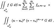
(22)
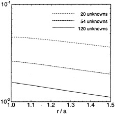
Figure 2: Relative error of ![]() (1) on the free surface, evaluated by the low-order panel method. The geometry is a bottom-mounted cylinder (radius=a, draft T=0.5a, wavenumber va=1) and the results are applicable along the radial line θ=π/4 relative to the upwave direction. The number of unknowns shown is for one quadrant of the body. The total number of panels on one quadrant waterline is 5, 9 and 15 respectively.
(1) on the free surface, evaluated by the low-order panel method. The geometry is a bottom-mounted cylinder (radius=a, draft T=0.5a, wavenumber va=1) and the results are applicable along the radial line θ=π/4 relative to the upwave direction. The number of unknowns shown is for one quadrant of the body. The total number of panels on one quadrant waterline is 5, 9 and 15 respectively.
where (ue,ve) is a central expansion point on the parametric space of the panel. The truncation index Nt is determined such that the first neglected term is of magnitude consistent with the other local errors.
3.3
Nonlinear methodology
When the integral equation (8) is used for the second- and third-order potentials, the principal modification is to evaluate the forcing function on the right-hand-side which involves integration over the free surface. As noted in §2, an appropriate procedure is to use numerical integration inside a circle of finite radius, and a semi-analytic analysis in the far field outside the same circle.
Since the inner integration is the most difficult computational task in the low-order panel method, we concentrate on it here and truncate the free surface at a specified partition radius r, and neglect the far field contribution in the forcing function. The resulting solutions are incomplete, but serve to demonstrate the advantages of HIPAN in solving the higher-order boundary-value problems. Another simplification which
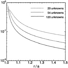
Figure 3: Relative error of ![]() on the free surface using the low-order panel method. See caption of Figure 2 for further details.
on the free surface using the low-order panel method. See caption of Figure 2 for further details.
is made here is to neglect the contribution to the third-order forcing function from the second-order potential. This is motivated by the long-wavelength approximation of Faltinsen et al. [4]. Both of these simplifications can be overcome in a relatively straightforward manner, using the same procedures as in the second-order version of WAMIT.
After solving for the first-order diffraction potential using (7), the same equation is used (with the factor 4π in the first term) to evaluate ![]() (1) at specified points on the free surface. A least-squares procedure is then used on an appropriate set of free-surface patches to approximate
(1) at specified points on the free surface. A least-squares procedure is then used on an appropriate set of free-surface patches to approximate ![]() (1) with B-spline expansions throughout the domain of the truncated free surface. The required first-and second- derivatives in the horizontal plane are then evaluated analytically. The required vertical derivatives are derived using the free-surface condition and Laplace's equation.
(1) with B-spline expansions throughout the domain of the truncated free surface. The required first-and second- derivatives in the horizontal plane are then evaluated analytically. The required vertical derivatives are derived using the free-surface condition and Laplace's equation.
Since the above procedure results (locally) in a polynomial form for the functions ![]() the integrals on the right-hand-side of equation (8) can be evaluated using the same algorithms described in Section 3.2. The subsequent procedure to solve (8) is essentially the same as for the first order potential.
the integrals on the right-hand-side of equation (8) can be evaluated using the same algorithms described in Section 3.2. The subsequent procedure to solve (8) is essentially the same as for the first order potential.
A fundamental advantage of this procedure is that it is relatively robust in the vicinity of the body waterline, by comparison to the low-order
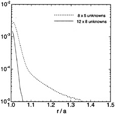
Figure 4: Relative error of ![]() (1) on the free surface, evaluated by HIPAN. The geometry and wavenumber are the same as in Figure 2. The number of panels and unknowns shown are for one quadrant of the body.
(1) on the free surface, evaluated by HIPAN. The geometry and wavenumber are the same as in Figure 2. The number of panels and unknowns shown are for one quadrant of the body.
panel method. To demonstrate this we first show results from WAMIT where the diffraction potential and its radial derivative are evaluated on the free surface, and compared with the analytical solution for a vertical circular cylinder. (These correspond more physically to the free-surface elevation and slope.)
The relative errors from the low-order computations are shown in Figures 2 & 3. In most cases the error is small, and can be reduced by increasing the number of panels, but close to the waterline intersection the derivative cannot be evaluated in a robust manner, as is true more generally near the body surface (Zhao & Faltinsen [22]). (To achieve maximum accuracy from WAMIT the radial derivative is evaluated using the source formulation, and along the normal to the body boundary at the mid-point of waterline elements.) Clearly this procedure cannot be used to evaluate the second derivatives near the body. In the second-order solution this problem can be minimized by using Gauss' theorem [11], but this approach cannot be extended to third order. In Figures 4 & 5 we show the corresponding results from HIPAN. Using a similar number of unknowns as in WAMIT, the relative error of the potential is about one order smaller near the body and decays more rapidly in the radial direction. The relative error of the radial derivative is
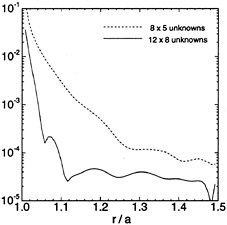
Figure 5: Relative error of ![]() on the free surface using HIPAN. See caption of Figure 4 for further details.
on the free surface using HIPAN. See caption of Figure 4 for further details.
substantially smaller as well. Near the waterline intersection the error is larger than away from the waterline intersection, but the problem is far less serious than in the low order panel method. By increasing the number of panels or the order of the potential on the body, the error of the potential decreases. While a loss of accuracy is inherent in obtaining derivatives by analytic differentiation of the polynomial representation of ![]() (1), it can be reduced with a suitable refinement of the B-spline characteristics on the body and on the free surface. The results shown in Figure 5 for
(1), it can be reduced with a suitable refinement of the B-spline characteristics on the body and on the free surface. The results shown in Figure 5 for ![]() use a B-spline representation where the potential is fit at 55×18 points on one quadrant of the free surface in the radial interval 1.0<r/a<1.5. This sector is sub-divided into 12×4 panels and B-splines of order 4 are used. This representation is sufficiently accurate so that the errors shown in Figure 5 are associated only with the first-order potential representation on the body surface. Similar results have been confirmed for the second derivative of the potential.
use a B-spline representation where the potential is fit at 55×18 points on one quadrant of the free surface in the radial interval 1.0<r/a<1.5. This sector is sub-divided into 12×4 panels and B-splines of order 4 are used. This representation is sufficiently accurate so that the errors shown in Figure 5 are associated only with the first-order potential representation on the body surface. Similar results have been confirmed for the second derivative of the potential.
The angular variation of the error using HIPAN is shown in Figure 6. It is interesting to note that the error is oscillatory, with maximum errors at the Gauss nodes and at the midpoints between these nodes. The error diminishes with increasing distance from the waterline intersection of the body, both radially and vertically. (Only the real part of the error is shown here since the imaginary component is relatively small.)
The free-surface Green function has a logarithmic singularity when the source and field points coincide on the free surface. This is presumed to be the dominant contribution to the errors discussed above. It is possible to treat this singularity in a semi-analytic manner, analogous to the technique described by Newman & Sclavounos [21]. This extension of HIPAN should further reduce the local error at the intersection.
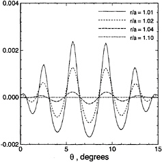
Figure 6: The error of the real part of ![]() (1) on the free surface using HIPAN with the order of the inner Gauss-Legendre quadratures equal to six. The solution is obtained at points adjacent to the first waterline segment, at the radii r. The geometry and wavenumber are the same as in Figure 2. The number of panels is 6×2 for one quadrant of the body and the potential B-splines are cubic.
(1) on the free surface using HIPAN with the order of the inner Gauss-Legendre quadratures equal to six. The solution is obtained at points adjacent to the first waterline segment, at the radii r. The geometry and wavenumber are the same as in Figure 2. The number of panels is 6×2 for one quadrant of the body and the potential B-splines are cubic.
4.
Results
A variety of examples are presented to demonstrate the robustness and efficiency of HIPAN. For the results presented, B-spline representation of patches are constructed by fitting points on the surface by a linear least-squares procedure. The geometric representations can be considered exact in relation to the approximation of the solutions for the velocity potentials. Generally we start with ‘coarse' representations of the potential using the same knot vectors (13) as in the geometry representation. More accurate potential representations are obtained using knot vectors which subdivide the intervals between consecutive geometry knots. We define panels as the physical surface corresponding to the parametric
Table 1: Definition of commonly used symbols.
|
Notation |
Quantity |
|
A |
wave amplitude |
|
a |
cylinder radius |
|
d |
half-distance between bodies |
|
g |
acceleration due to gravity |
|
T |
cylinder draft |
|
λ |
wavelength |
|
v |
wavenumber |
|
ρ |
fluid density |
|
ω |
radian frequency |
space between consecutive knots of the potential B-splines. Therefore, the number of panels refers to the product, M1×N1 for a body described by one patch, or the sum of products ∑pMp×Np for a body described by several patches.
The most significant errors in this scheme are associated with the order (Ng) of the product Gauss-Legendre rule for the outer integration (Galerkin), and the limitations of the potential B-spline approximation (15). The latter is controlled by the total number of splines used, their degree, and their distribution over the region. Since these factors are independent, a simple but effective indicator of the approximating ability of (15) and the ensuing computational effort is the number of unknowns (19) involved. Secondary sources of error include the truncated normal derivative expansion, the amplification of errors in the solution due to an ill-conditioned linear system of equations, inaccuracies in the B-spline surface patches, and lack of continuity across patches.
Table 1 defines the notation used in presenting the results below.
4.1
First-order results
As the first example we evaluate the surge added-mass and damping coefficients for a floating hemisphere, where the benchmark results of Hulme [9] are available for comparison. One quadrant of the hemisphere is modelled as a patch (![]() =1). Symmetry is used to restrict the unknown solution to this patch, where the potential is represented by a cubic (k=4) B-spline expansion. The expansion (22) for the normal derivative is truncated at degree Nt=4. The outer integration is an Ng×Ng=3×3 Gauss rule. Figure 7 compares the HIPAN results with those
=1). Symmetry is used to restrict the unknown solution to this patch, where the potential is represented by a cubic (k=4) B-spline expansion. The expansion (22) for the normal derivative is truncated at degree Nt=4. The outer integration is an Ng×Ng=3×3 Gauss rule. Figure 7 compares the HIPAN results with those
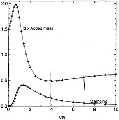
Figure 7: The surge added-mass and damping coefficients for a floating hemisphere, normalized by the factors 2πρa3/3 and 2πωρa3/3, respectively. The solid triangles are results from Hulme, and the dotted and solid lines corresp ond to computations with 2×2 and 3×3 panels per quadrant respectively.
of Hulme [9]. Two sets of results are plotted, corresponding to discretizations with M1×N1=2×2 and 3×3 panels, corresponding to 5×5 and 6×6 unknowns. The corresponding curves are practically indistinguishable, except in the vicinity of the irregular frequencies. The bandwidth of the irregular frequencies is very narrow, particularly for the finer discretization.
To illustrate the application to a more complicated problem we next consider the surge exciting force on the Snorre TLP shown in Figure 1. Each quadrant of the TLP is represented by 35 patches. These computations are performed in a finite water depth (For the dimensions and depth see [12]). Two discretizations are used for the potential, labelled ‘coarse' and ‘fine'. The coarse discretization is shown in Figure 1, with panels as large as the entire pontoon side. The fine discretization corresponds to subdividing each panel of the coarse set into four smaller panels. Figure 8 compares the first-order surge exciting force on the TLP as computed by the present method and by the low-order panel method WAMIT. The graphical agreement with WAMIT is clear. The use of linear potential B-splines for the coarse case and cubic splines for the fine case, involve 164 and 989 unknowns per quadrant respectively.
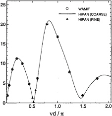
Figure 8: Surge exciting force on the Snorre TLP, normalized by ρgAa2.
We observe from Figure 8 that the maximum value of the surge exciting force occurs near vd/π=1, where the wavelength λ is equal to the column spacing 2d, and minimum values occur near the points where λ/2d is equal to 0.5 and 1.5. These correspond respectively to the condition where the local phase of the incident waves is the same at both pairs of columns, and where the waves are out of phase. This simple explanation, which is well known, essentially follows from considering only the Froude-Krilov exciting force and neglecting the scattered pressure field. The importance of the latter, and the small shift of the maximum force to vd/π![]() 0.86 corresponding to λ/2d
0.86 corresponding to λ/2d![]() 1.16, is illuminated by considering a long array of N circular cylinders in a single row, with equal spacing 2d between adjacent cylinders.
1.16, is illuminated by considering a long array of N circular cylinders in a single row, with equal spacing 2d between adjacent cylinders.
The first application of HIPAN to a long array was performed for the case of bottom-mounted circular cylinders in a finite water depth (Maniar & Newman [17]), to permit comparison with the semi-analytic interaction theory of Linton & Evans [13]. Computations were performed with up to 100 cylinders, revealing a singularly large surge exciting force (parallel to the array) acting locally on each cylinder, at the critical wavenumber where trapped waves occur for a single cylinder in a channel (Linton & Evans [14]). For N=100 and a/d=0.5 the local surge force on cylinders near the center of the array is about 35 times the magnitude of the force on a single isolated cylinder!
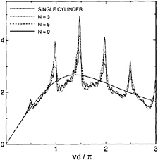
Figure 9: The magnitude of the exciting force in head seas on the first cylinder in an array of N truncated circular cylinders. The draft is equal to the radius a and the separation between adjacent cylinder centers is 2d=10a.
To further illustrate this phenomenon we consider the head-sea diffraction by a periodic array of N truncated circular cylinders, of radius a and draft T=a, with the centers separated by five diameters (2d=10a). Figure 9 shows the magnitude of the exciting force on the first cylinder, for N=1, 3, 5, 9. Sharp peaks are evident when vd/π is equal to an integer or an integer plus one half. The peak values increase with increasing N, whereas the bandwidth decreases. Similar behavior has been observed with arrays of floating hemispheres and spheroids.
Figure 10 shows the magnitude of the exciting force on each cylinder in a long array with N=100 elements, at the critical wavenumber near vd/π=1. In this case the force increases along the first 20% of the array, and diminishes thereafter, with substantial sheltering only present near the leeward end. The maximum force is amplified by a factor of four times the force on a single cylinder, and total integrated force on the entire array is about two times the simple estimate based on one cylinder.
Computations of the free-surface elevation show that local ‘sloshing modes' of large amplitude exist at the same wavenumbers where the exciting force on each cylinder is large. The first mode, near vd/π=1/2, corresponds to the trapped mode for a single cylinder in a channel
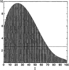
Figure 10: The distribution of the exciting force along an array of 100 truncated circular cylinders in head seas for vd/π=0.988. The cylinder at the head of the array corresponds to I=1. The horizontal dashed line indicates the magnitude of the exciting force on a single isolated cylinder.
with rigid walls; in this case the phase of the sloshing mode and local force differs by 180° between adjacent cylinders, and the total integrated force on the array is relatively small. The second mode, near vd/π=1, appears to correspond to a trapped mode for a single cylinder in a channel with ‘Dirichlet walls' where the potential is zero; here the motion at adjacent cylinders is in phase and the total integrated force is large. These trapped modes correspond to eigensolutions of the beam-sea diffraction problem in the limit N → ∞. It appears that similar ‘trapped' modes occur for the higher wavenumbers, corresponding to the successive peaks in Figure 9.
To address the issue of computational efficiency, Table 2 compares the number of unknowns required and execution time, for equivalent accuracy, using HIPAN and using the conventional low-order panel method. Two applications are included in this comparison, the heave exciting force on a single truncated circular cylinder and the vertical mean drift force on a submerged sphere. The times reported in the two cases are for a spectrum of 8 and 6 wavenumbers respectively. For a 1.0%–0.1% relative error, the B-spline higher-order method is 10–200 times faster than the constant panel method. If greater accuracy is required, or for more complicated bodies,
Table 2: Comparison of the number of unknowns and run times required to obtain equivalent accuracy, for HIPAN (H) and the low-order panel program WAMIT (W). The results in the upper table are for the surge exciting force on a truncated circular cylinder, and in the lower table for the vertical second-order drift force on a submerged sphere in finite depth. The figures in parenthesis are for cubic B-splines; the other HIPAN results are for linear B-splines. The last column shows the typical execution time, per wavenumber, on a DEC Alpha 3000/700 workstation.
|
Relative Error |
# of unknowns per quadrant |
Time [seconds] |
|
|
W |
1% |
512 |
44 |
|
H |
1% |
16 (48) |
1 (3) |
|
W |
0.1% |
2048 |
1140 |
|
H |
0.1% |
32 (72) |
4 (17) |
|
Relative Error |
# of unknowns |
Time [seconds] |
|
|
W |
0.6 ~ 3% |
800/quadrant |
637 |
|
H |
1% |
–(49)/half-body |
–(10) |
|
W |
0.05 ~ 1% |
3081/quadrant |
11428 |
|
H |
0.1% |
–(121)/half-body |
–(108) |
the ratio of the computational effort between the two methods is even larger due to the faster rate of convergence of the higher-order method.
A comparison of the accuracy and convergence of the two programs is shown in Figure 11, for the surge exciting force on the Snorre TLP plotted in Figure 8. This example is intended to provide a more practical illustration of the computational efficiency of HIPAN, but it is somewhat difficult to study the very small errors involved in a systematic manner due to the complexity of the geometry and the difficulty of deriving benchmark values. For WAMIT the benchmarks are established by extrapolation of the computations shown. In the case of HIPAN the benchmark is a separate run with cubic B-splines and a greater number of unknowns. Uncertainties in the benchmark may be responsible for the inconsistent convergence rates shown. Nevertheless it is clear that the average errors experienced with HIPAN are 10 to 100 times smaller than with WAMIT, with similar numbers of unknowns.
The rate of convergence depends primarily on the order of the (potential) splines, their distri-
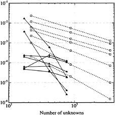
Figure 11: The computational error vs. the number of unknowns for the surge exciting force on the Snorre TLP. Each dashed line corresponds to WAMIT computations with (218, 872, 3488) unknowns. Each solid line corresponds to analogous computations from HIPAN using linear B-splines with (171, 413, 761) unknowns. Each line represents a discrete value of the wavenumber in the range shown in Figure 8.
bution on the body (governed by the use of uniform or nonuniform knot vectors) and the specific physical problem. Our experience to date indicates that for smooth bodies with uniform knots, the error in integrated quantities is proportional to u–α where u is the total number of unknowns (19) and the exponent α ![]() 2k–1 (k=order of the splines). In the presence of flow singularities for bodies with corners, the use of higher-order splines based on uniformly distributed knots may result in linear convergence only. In such cases, the convergence rate is expected to improve with the use of nonuniform splines.
2k–1 (k=order of the splines). In the presence of flow singularities for bodies with corners, the use of higher-order splines based on uniformly distributed knots may result in linear convergence only. In such cases, the convergence rate is expected to improve with the use of nonuniform splines.
4.2
The second-order solution
Preliminary computations are presented here to verify the effectiveness of HIPAN in solving for the second-order potential. The problem considered is the second-order diffraction by a truncated circular cylinder with radius a and draft T=6a. Cosine spacing is used to discretize the cylinder and a uniform discretization is used on the free surface. The free-surface integration in (8) is truncated at a finite radius r=6a to simplify the computations. The resulting potential
Table 3: The second-order horizontal force as computed by HIPAN and WAMIT. For the results in column 2, 96+86 panels are used on the body and the free surface for HIPAN and 2688+7680 panels for WAMIT. Finer discretizations are used in column 3, with 160+134 panels for HIPAN and 9984+30720 panels for WAMIT.
|
va |
|
|
|
0.10 |
–0.07969 |
–0.07969 |
|
0.15 |
–0.32143 |
–0.32145 |
|
0.20 |
–0.47781 |
–0.47778 |
|
va |
|
|
|
0.10 |
–0.0760 |
–0.0783 |
|
0.15 |
–0.3107 |
–0.3177 |
|
0.20 |
–0.4568 |
–0.4699 |
|
va |
|
|
|
0.10 |
–0.05968 |
–0.05967 |
|
0.15 |
0.00932 |
0.00931 |
|
0.20 |
0.36915 |
0.36921 |
|
va |
|
|
|
0.10 |
–0.0460 |
–0.0532 |
|
0.15 |
0.0321 |
0.0208 |
|
0.20 |
0.3946 |
0.3811 |
is incomplete, but since the integration over the truncated free-surface is the most computationally expensive task, we are able to evaluate the effectiveness of HIPAN without the additional effort associated with the far-field integration.
Table 3 shows the resulting second-order horizontal force, for three wavenumbers and two discretizations. Also shown are the corresponding results evaluated from the low-order panel program WAMIT. For the two B-spline discretizations the HIPAN results are converged to 4–5 decimals. The WAMIT results converge more slowly, although the number of panels is much larger.
4.3
The third-order solution
As noted in the Introduction, the problem of ‘ringing' has focused attention on third-order wave loads, particularly the high-frequency components in a spectrum or the third-harmonic in a regular wave system. Two complementary studies of the third-harmonic force on a circular cylinder have been made by Faltinsen et al. [4] (‘FNV') and by Malenica & Molin [15] (‘M&M'), using different assumptions and boundary conditions. While the magnitude of the third-harmonic force is similar in these two works, the phase is opposite
Table 4: Real (top) and imaginary (bottom) parts of the third-harmonic force based on the long-wavelength approximation. The numerical solution is obtained by truncating the free surface at the radius r/a.
|
va |
FNV |
r/a=6 |
r/a=12 |
|
0.025 |
–9.817E-04 |
–8.721E-04 |
–8.661E-04 |
|
0.05 |
–3.927E-03 |
–3.610E-03 |
–3.616E-03 |
|
0.10 |
–1.571E-02 |
–1.582E-02 |
–1.606E-02 |
|
0.15 |
–3.534E-02 |
–3.894E-02 |
–3.931E-02 |
|
0.20 |
–6.283E-02 |
–7.321E-02 |
–7.204E-02 |
|
0.025 |
0.00 |
4.017E-07 |
3.480E-07 |
|
0.05 |
0.00 |
7.600E-06 |
4.447E-06 |
|
0.10 |
0.00 |
1.101E-04 |
–6.292E-05 |
|
0.15 |
0.00 |
9.586E-05 |
–1.426E-03 |
|
0.20 |
0.00 |
–2.178E-03 |
–8.090E-03 |
over the most important regime (0.1<va<0.4).
We are using HIPAN to develop a more general solution of the third-order problem which is applicable to practical body shapes including the TLP. This computational approach can be developed following the boundary conditions and assumptions of either FNV or M&M, so that it is possible to develop independent results for comparison with their more analytical solutions. As a first step we simplify the solution of the third-order potential by neglecting both the far-field forcing on the free surface (as in the second-order results described above) and also the contribution to the third-order forcing function due to the second-order potential. Both of these simplifying assumptions are justified asymptotically in the long-wavelength regime, as shown by FNV.
The results presented here are for the truncated cylinder with draft T=6a. This is considered to be sufficiently deep so that comparison can be made with the infinitely deep cylinder of FNV.
First, following the long-wavelength approximations of FNV, only the second term in the forcing function (6) is retained, and the Green function G=1/r+1/r′ is used to solve for the third-order potential. The resulting third-harmonic force is tabulated in Table 4 for two values of the truncation radius on the free surface, and compared with the corresponding force from the FNV analysis. The computations are relatively insensitive to the truncation radius, since the forcing is confined to the near field in the long-wavelength approximation. The agreement
Table 5: The real (top) and the imaginary (bottom) part of third-harmonic force based on the diffraction analysis.
|
va |
r/a=6 |
r/a=9 |
r/a =12 |
|
0.025 |
–1.182E-03 |
–1.161E-03 |
–1.163E-03 |
|
0.05 |
–6.469E-03 |
–6.317E-03 |
–6.113E-03 |
|
0.10 |
1.013E-03 |
–3.141E-03 |
–3.354E-03 |
|
0.15 |
3.607E-02 |
4.447E-02 |
3.031E-02 |
|
0.20 |
7.451E-02 |
7.217E-02 |
9.383E-02 |
|
0.025 |
1.158E-04 |
7.391E-05 |
6.085E-05 |
|
0.05 |
3.701E-03 |
3.805E-03 |
3.668E-03 |
|
0.10 |
3.748E-02 |
3.410E-02 |
3.907E-02 |
|
0.15 |
5.654E-02 |
7.300E-02 |
6.284E-02 |
|
0.20 |
9.317E-02 |
6.980E-02 |
6.644E-02 |
with the FNV results is reasonable, considering the finite draft of the cylinder. The imaginary part of the force is zero in the FNV analysis, and relatively small in the computed results.
To correspond more closely with the diffraction analysis of M&M, the procedure described above has been extended by including all of the contributions from the first-order potential to the third-order forcing function (6), and by using the complete free-surface Green function. The results obtained in this manner are listed in Table 5. In this case the convergence with truncation radius is somewhat less satisfactory, except for the longest wavelength (va=0.025). Referring to the results for the largest radius, in the last column, and comparing these with the corresponding results in 4, it appears that the real component changes sign in the same manner as in the results of M&M, and the imaginary component is significant for all but the longest wavelength. These preliminary results appear to support the conclusion of M&M that diffraction effects are significant in the regime va>0.1.
5.
Conclusions
The higher-order panel method described here makes use of B-splines to describe both the body geometry and the velocity potential on the body surface. The accuracy and efficiency of B-splines means that the description of the geometry can be practically exact, and the representations of the velocity potential and its derivatives are continuous. Thus wave radiation and diffraction problems can be analyzed more efficiently than with the low-order panel method, and it is possible to develop second- and third-order solutions with a more robust evaluation of the inhomogeneous forcing function on the free surface.
A variety of examples have been used to illustrate the results of this method, based on the program HIPAN. For first-order wave loads comparisons of run time and accuracy are made with the low-order program WAMIT. One indication of accuracy is the very narrow bandwidth of the irregular frequencies in the results for a floating hemisphere. The computational efficiency of HIPAN is evident especially for applications where a relatively large number of panels are required. The long periodic array with up to 100 separate cylinders is used to illustrate the feasibility of analyzing a large complex structure which would be difficult or impractical with low-order programs.
The tests for long periodic arrays were originally intended to test the computational capabilities of HIPAN, but the results have given us a more complete understanding of the role of trapped wave modes. In particular, finite arrays of bodies are shown to experience relatively large wave loads at certain critical wavenumbers. These correspond to the existence of trapped modes, which have been associated in the past with wave diffraction by a single body in a channel of finite width.
The higher-order method is particularly advantageous in the analysis of second- and third-order wave loads. In these problems the computational cost is relatively high, and thus the efficiency of the B-spline technique is more significant. More fundamentally, the continuity of the resulting solution makes it possible to evaluate the free-surface forcing effects in a robust manner, particularly in the vicinity of the body/free-surface intersection. Another possible application where this feature may be useful is in the analysis of wave-drift damping [5].
One more possible advantage of the continuous B-spline representation is in applying the resulting wave loads to a structural-analysis code. In finite-element structural analysis it is necessary to use a refined discretization, for example with smaller elements in regions of stress concentration. This mismatch between appropriate discretizations for the hydrodynamic and structural analyses can be overcome easily if the wave loads are described continuously on the body surface.
The problems described here are based on perturbation expansions in the frequency domain,
and on the use of the special Green functions which satisfy the linearized free-surface boundary condition with harmonic time dependence. Similar higher-order techniques can be applied in the context of other applications of panel methods. One example is the solution of the double-body flow past a ship hull, where HIPAN has been used by Bingham & Maniar [1] to evaluate the so-called m-terms which involve second derivatives of the velocity potential. Another example is in the time-domain analysis of wave-body interactions, where parallel work is now underway using the transient free-surface Green function. Similar techniques may be applied also to linear and non-linear wave problems where Rankine Green functions are distributed on both the body and free surface.
An important practical consideration is the difficulty of using HIPAN. Unlike low-order panel methods where the geometry is described by a set of vertices, or points in Cartesian space situated on the body surface, HIPAN requires a set of B-spline control points which are relatively small in number, but more abstract to interpret. In practice, specialized pre-processor programs must be used in both cases, and we anticipate that suitable software will be developed so that B-splines can be used by practicing engineers with no more effort than is presently required to input the coordinates of panel vertices.
One feasible extension which offers substantial benefit in terms of ‘user-friendliness' is to automate the process of testing for numerical convergence. In conventional panel methods there is no method for determining a priori if the panel representation of the body is sufficiently accurate in relation to the hydrodynamic parameters of interest; this question can only be answered by repeating the analysis with smaller panels and testing the results for convergence. Several examples of this procedure are described by Newman & Lee [20]. Assuming the B-spline description of a body surface is practically exact, it is relatively straightforward to automatically subdivide patches, or use B-splines of increasing order to represent the potential, and to test these results for convergence within the program. With such a procedure implemented it would be feasible for a user to specify the required precision of the hydrodynamic parameters of interest, and the program would then ensure that this precision is achieved without the need for the user to perform laborious convergence tests.
In the initial development of HIPAN we were attracted by the flexibility and elegance of B-splines. However they are but one of a large number of possible basis functions which might be used. An obvious extension is to consider rational B-splines with nonuniform knot-vectors (NURBS). In HIPAN the equivalence of B-splines to polynomials is exploited in the evaluation of the influence functions, but it appears that this restriction can be removed without substantial complication or loss of computational efficiency. It now seems feasible to develop a more general panel method where the description of the body surface is completely general, provided only that it is defined by a set of algorithms which correspond respectively to sub-regions or ‘patches’. The only restriction is that the Cartesian coordinates of points on each patch can be transformed by a continuous mapping function onto a rectangular parametric coordinate space. The complete submerged surface of the body would then be described by the union of these patches. In this manner we envisage an extension of HIPAN which is applicable to any continuously-defined body shape, retaining the B-spline representation only for the solution on each patch and leaving it to the user to define the body geometry in whatever manner is most convenient and exact.
Acknowledgment
This work was conducted under a Joint Industry Project. The sponsors have included the Chevron Petroleum Technology Company, Conoco, David Taylor Research Center, Exxon Production Research, Mobil Oil Company, National Research Council of Canada, Norsk Hydro, Offshore Technology Research Center, Petrobrás, Saga Petroleum, Shell Development Company, Statoil, and Det Norske Veritas. Additional support was provided by the National Science Foundation, Grant 9416096-CTS.
References
[1] Bingham, H.B. & Maniar, H., “Calculating the double body m-terms with a higher order B-spline based panel method”, Eleventh International Workshop on Water Waves and Floating Bodies . Hamburg, 1996.
[2] DeBoor, C., A Practical Guide to Splines, Applied Mathematical Sciences, 27, Springer-Verlag, 1978.
[3] Eatock Taylor R. & Chau F.P. “Wave diffraction theory—some developments in linear and nonlinear theory,” J. of Offshore Mechanics and Arctic Engineering, 114, 1992, pp. 185–194.
[4] Faltinsen, O.M., Newman, J.N. & Vinje, T., “Nonlinear wave loads on a slender vertical cylinder.” J. Fluid Mech., 289, 1995, pp. 179–198.
[5] Grue, J., & Palm, E., “The mean drift force and yaw moment on marine structures in waves and current.” J. Fluid Mech., 250, 1993, pp. 121–142.
[6] Herfjord, K. & Nielsen, F.G., “A comparative study on computed motion response for floating production platforms: Discussion of practical procedures.”, Proc. 6th. International Conf. Behaviour of Offshore Structures (BOSS '92), Vol. 1, London, 1992.
[7] Hess, J.L. & Smith, A.M.O., “Calculation of nonlifting potential flow about arbitrary three-dimensional bodies.”, J. Ship Research, 8, 1964, pp. 22–44.
[8] Hsin, C.-Y., Kerwin, J.E. & Newman, J.N., “A Higher-Order Panel Method Based on B-splines”, Proceedings of the Sixth International Conference on Numerical Ship Hydrodynamics, Iowa City, 1993.
[9] Hulme, A., “The wave forces acting on a floating hemisphere undergoing forced periodic oscillations.”, J. Fluid Mech., 121, 1982, pp. 443–463.
[10] Korsmeyer, F.T., Lee, C.-H., Newman, J.N. &; Sclavounos, P.D., “The analysis of wave interactions with Tension-Leg Platforms”, OMAE Conference, Houston, 1988.
[11] Lee, C.-H., WAMIT Theory Manual, Report No. 95–2, Dept. of Ocean Engg., Massachusetts Institute of Technology, 1995.
[12] Lee, C.-H. & Newman, J.N., “Second-Order wave effects on offshore structures.”, Proc. 7th. International Conf. Behaviour of Offshore Structures (BOSS '94) , Vol. 2, Pergamon, 1994.
[13] Linton, C.M. & Evans, D.V., “The interaction of waves with arrays of vertical circular cylinders ”, J. Fluid Mech., 215, 1990, pp. 549–569.
[14] Linton, C.M. & Evans, D.V., “The radiation and scattering of surface waves by a vertical circular cylinder in a channel”, Phil. Trans. R. Soc. Lond. A, 338, 1992, pp. 325– 357.
[15] Malenica, Š. & Molin, B., “Third-harmonic wave diffraction by a vertical cylinder.” J. Fluid Mech., 302, 1995, pp. 203–229.
[16] Maniar, H., A three dimensional higher order panel method based on B-splines, Ph.D. thesis, Massachusetts Institute of Technology, 1995.
[17] Maniar, H. & Newman, J.N., “Wave diffraction by a long array of circular cylinders”, Eleventh International Workshop on Water Waves and Floating Bodies . Hamburg, 1996.
[18] Molin B. & Chen X.B. 1990 Vertical resonant motions of tension leg platforms, Unpublished report, Institut Français du Pétrole, Paris.
[19] Newman, J.N., “The approximation of free-surface Green functions”, in Wave Asymptotics, P.A.Martin & G.R.Wickham, editors, Cambridge University Press, 1992, pp. 107–135.
[20] Newman, J.N., & Lee, C.-H., “Sensitivity of wave loads to the discretization of bodies.”, Proc. 6th. Conf. on the Behaviour of Offshore Structures (BOSS '92), Vol. 1, London, 1992.
[21] Newman, J.N., & Sclavounos, P.D., “The computation of wave loads on large offshore structures,” Proc. 5th. Conf. on the Behaviour of Offshore Structures (BOSS ‘88), Trondheim, 1988.
[22] Zhao, R. & Faltinsen, O., “A discussion of the m-terms in the wave-body interaction problem”, Fourth International Workshop on Water Waves and Floating Bodies. Øystese, 1989.
DISCUSSION
L.J.Doctors
University of New South Wales, Australia
I would like first to say how much I enjoyed the presentation of this work. I believe the careful analysis of the errors, such as that shown in Figures 2 through 6, is a most important and useful aspect of such research because it provides confidence in the method and the computer program.
Figure 7 shows the added-mass and damping coefficients for a floating hemisphere. The well-known problem of the misbehavior of the panel method in the neighborhood of the irregular frequencies is displayed there. Could the authors comment on how they eliminate this difficulty in practical applications of their work? In my own two-dimensional panel-method analysis of ship sections for a strip-theory ship-motion computer program, I have found the use of a “lid” on the internal free surface of a surface-piercing section to be both easy to program and very effective. Either a stationary or a moving lid seems to be equally good. This is detailed in the publication: Doctors, L.J., “Application of the Boundary-Element Method to Bodies Oscillating near a Free Surface,” Computational Fluid Dynamics, Proc. Intl Symposium on Computational Fluid Dynamics, Sydney, Elsevier Science Publishers B.V., Amsterdam, pp. 377–386 (1988).
AUTHORS' REPLY
We thank Dr. Doctors kindly for his comments.
While the irregular frequencies are a set of isolated frequencies in the continuous problem, their effects in the discrete problem appear as erroneous solutions in the vicinity of those frequencies. The frequency bandwidth of the erroneous solution decreases as the discrete formulation of the problem is made more exact, either by increasing the number of panels in a low-order method or by using higher-order algorithms. The latter is illustrated by Figure 7, where the bandwidth is very narrow compared to typical results from low-order panel methods. Thus, the results in this Figure demonstrate the more accurate approximation to the continuous problem which can be achieved using the higher-order panel method.
There are several known techniques to eliminate the effects of irregular frequencies. Our own experience with the low-order panel method also suggested that putting a “lid” on the interior free surface is effective from the computational point of view. We have refined this technique and used it in the low-order panel code WAMIT to remove the irregular frequency effects from the first- and second-order nonlinear solution. This work was reported in Lee, Newman, and Zhu (1996). The same technique can be easily applied to the higher-order panel method but we have not done so, partly to illustrate the much narrower bandwidth that is present in the latter method.
ADDITIONAL REFERENCE
[24] Lee, C.-H., Newman, J.N., and Zhu, X. “An extended boundary integral equation for the removal of the irregular frequency effect,” Int. J. for Numerical Methods in Fluids (in print).
DISCUSSION
W.W.Shultz
University of Michigan, USA
-
Higher-order panels are known to be more susceptible to singularities. Have you noticed such problems at the corners? What constraints do you put on the patches?
-
The lines midway between cylinders look like appropriate locations to apply periodic boundary conditions if the wavenumber in the in-line cylinder direction is properly chosen. Then, couldn't waves come in many directions?
AUTHORS' REPLY
-
We do not place any constraints on the solution at the boundaries between contiguous patches. We find that the potential is practically continuous at these boundaries, even in cases where there is an external corner flow. Figure 12, reproduced from [16], illustrates this in the case of the streaming flow past a cube (without a free surface). The equipotential lines in this figure appear to be smooth and continuous within graphical accuracy, except for a small discontinuity which is evident near the corner where the three edges meet.
-
For a long array, the solution is nearly periodic along the array, with a constant phase shift between adjacent cylinders. Away from the resonant peaks, this phase shift is governed by the longitudinal component of the incident-wave wavenumber and by the cylinder spacing, as assumed by Linton & Evans [23]. However, at the resonant peaks, where the “sloshing modes” are dominant, the phase shift is either zero (Dirchlet modes), or 180° (Neumann modes), in accordance with the requirement that the sloshing modes be continuous between adjacent cylinders. In the latter case, the direction of the incident waves is irrelevant, as suggested by Professor Schultz.
ADDITIONAL REFERENCE
[23] Linton, C.M. & Evans, D.V., “The interaction of waves with a row of circular cylinders,” J. Fluid Mech., 251, 1993, pp. 687–708.
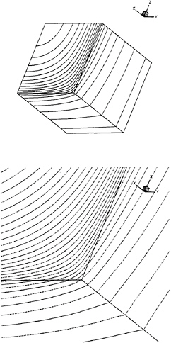
FIGURE 12: Equipotential contours on an octant of a translating cube. Each side of the octant is a patch and discretized by 8×8 panels/patch. The lower figure is a close-up of the corner showing continuity across patches.


