
Advances in Panel Methods
H.Söding (Institut für Schiffbau, Germany)
Abstract
In spite of improving computers, a number of inviscid CFD problems still suffer from excessive storage and/or computing time requirements. Examples are detailed pressure distributions on propellers in a wake field, ship wave effects for low Froude numbers, ship encounters in a channel, 3D seakeeping problems and instationary flows which are not time-harmonic. Three measures to reduce the computer requirements for such problems are demonstrated: the multigrid method, panel clustering, and a new higher-order panel method. Further, the ‘patch' method is presented which allows more accurate resistance computations without increasing time or unknowns.
1.
Introduction
Computational fluid dynamics (CFD) supports to an increasing extent model tests. An important field are “wave-resistance” computations, which use almost exclusively Rankine panel methods to analyse local flow details, to optimise local hull shapes (especially the bulbous bow) and to align of shaft brackets etc. [1], [2]. However, the resistance is not predicted with sufficient accuracy, and reliability to substitute model experiments. Ordinary higher-order panels increase accuracy for simple test cases (spheroids, Wigley hulls, etc.), but failed only recently to show consistent improvements for real ships in an investigation at our institute, [3]. For slow ships (tankers, inland water vessels), due to time and storage limitations the free-surface grids are chosen often too coarse to resolve the short waves.
Panel methods gain in importance for manoeuvring calculations, [4], [5]. Due to the usually low speeds involved and the asymmetry of the flow, problems with a sufficiently fine and extended discretisation are even more severe. Two-ship encounter simulations are generally not tackled using Rankine panel methods due to the large number of unknowns required. Seakeeping computations using Rankine panels for bodies with forward speed were reviewed this year by [6]. Here generally the covered free-surface area is larger than in wave-resistance computations, and the grid spacing should be finer to cover a wide band-width of wave lengths that may appear in one computation.
In summary, various hydrodynamical computations of practical relevance would benefit from techniques that allow to use more panels without increasing storage and CPU time requirements. Multigrid and cluster techniques can serve this purpose. For a fixed discretisation, the accuracy can be significantly improved by the ‘patch' method. Also a new higher-order panel technique with numerical integration appears promising. Advantages will be demonstrated here for steady double-body flows and one example of a free-surface flow, but all techniques are suitable for steady and unsteady flows with and without a free-surface.
2.
Patch Method
The aim of the patch method [7] is to increase the accuracy of pressure forces and velocity averages over a patch on a body surface compared to the usual first-order panel methods, without introducing a finer discretisation or the complexity of higher-order panel methods. For a given discretisation, the computing time of the panel method and the patch method are about the same, and so are the program complexity and the accuracy of velocities at single points.
Consider an arbitrary body in an infinite ideal fluid (double-body flow). The boundary condi-
tion on the hull (body surface) is that no water flows through the hull. The usual approach in boundary element methods discretises the hull into a number of elements (panels). The boundary condition is then exactly enforced at one point, the collocation point, located approximately at the panel center.
In the ‘patch' method, on the other hand, the total flow through each surface element (patch), and not just at its center, is made to vanish. Using sources distributed over plane or curved panels would lead to complicated integrations; therefore in the patch method simple point sources are used. They are located within the body near to the patch centres. The distance between patch centre and source point may be chosen as the minimum of the following lengths:
Square root of patch area;
1/3 of the local body breadth;
1/2 the radius of longitudinal curvature;
1/2 the radius of transverse curvature.
The results are not sensitive to this distance; in many applications simply 1/10 of the patch length is used.
In the panel method, velocity and pressure can be determined on the hull directly only at the panel centres; at other points, interpolation has to be used. Pressure forces are, typically, determined by multiplying the pressure at the panel centre with the panel area. The patch method aims just to improve this force formula. In the patch method, potential and velocity are determined at the patch corners instead of at the patch centre, i.e. at a reasonable distance from all point sources. The potential at the patch corners allows a better approximation of the average velocity within the patch than the value at the panel centre, and combining the potential and the velocity at the patch corners allows to determine an accurate average of the pressure within the patch.
For a body in uniform flow to negative x direction, the potential is
(1)
U is the speed of the uniform flow, σ the source strength, G the potential of a Rankine point source:
G=ln r in 2D, and G=–1/r in 3D, (2)
where ![]() is the distance between field point
is the distance between field point ![]() and source point
and source point ![]()
Let Mi be the outflow through a patch induced by a point source of unit strength. Then the zero-flow condition for a patch is
(3)
Here ![]() is the outward normal on the hull, index x (and later z) designates the respective component of
is the outward normal on the hull, index x (and later z) designates the respective component of ![]() and Anx is the projection of the patch area on a plane x=constant (with appropriate sign); for the 2d case of Fig.1: Anx=yA–yB.
and Anx is the projection of the patch area on a plane x=constant (with appropriate sign); for the 2d case of Fig.1: Anx=yA–yB.
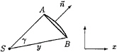
Fig. 1: Patch (from A to B) and source point S
2.1
2-d Formulation
The outflow due to the unit source potential In r into all directions is 2π. The outflow M due to the unit source in ![]() passing through the patch in Fig.1 is thus equal to the angle γ under which the patch is seen from
passing through the patch in Fig.1 is thus equal to the angle γ under which the patch is seen from ![]() —both for a straight and a curved patch. If
—both for a straight and a curved patch. If ![]() and
and ![]() are the vectors from S to A and B respectively, γ is easily determined from the vector and scalar products of
are the vectors from S to A and B respectively, γ is easily determined from the vector and scalar products of ![]() and
and ![]() :
:
(4)
From the value of the potential ![]() at the end points A and B, the average modulus
at the end points A and B, the average modulus ![]() of the velocity
of the velocity ![]() is found as |
is found as |![]() A–
A–![]() B|/l, where l ist the length of the patch. The direction of
B|/l, where l ist the length of the patch. The direction of ![]() is parallel to the contour. The velocity
is parallel to the contour. The velocity ![]() at the end points, designated here as
at the end points, designated here as ![]() is found as
is found as ![]() .
.
The pressure force on a straight patch is
(5)
where v, the modulus of ![]() is not constant. To evaluate this expression, v is approximated by the second-order polynomial giving the known values vA, vB and
is not constant. To evaluate this expression, v is approximated by the second-order polynomial giving the known values vA, vB and ![]() :
:
v=vA+(6![]() –4vA–2vB)t+3(vA+vB–2
–4vA–2vB)t+3(vA+vB–2![]() )t2 (6)
)t2 (6)
t is the tangential coordinate directed from A to B. From this expression follows the integral in (5):
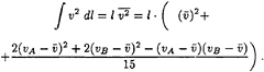
(7)
As a test case, a symmetric profile with circular nose, parabolic run and a sharp tail, with thickness-chord ratio of 2, was investigated at zero angle of attack. The resistance, which should be zero due to d'Alembert's paradox, is used to indicate the error. (A test body should not be symmetric in x to avoid cancellation of the discretisation error.) The panel method used for comparison applied straight elements of constant source strength, a collocation scheme and constant pressure over each element.
Table I: Relative resistance (=error) for a foil-shaped profile; comparison of patch method (PTM) with first-order panel method (OPM)
|
elem. no. |
12 |
24 |
48 |
96 |
192 |
|
PTM |
17% |
13% |
5% |
1.4% |
0.5% |
|
OPM |
100% |
47% |
22% |
10% |
5% |
The patch method proved to be about 5 times more accurate than the panel method, Table I. In other words, only 1/4 of the number of elements of the ordinary panel method sufficed for the patch method to obtain the same force accuracy.
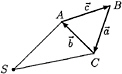
Fig. 2: Source point S and patch ABC
2.2
3-d Formulation
The outflow due to the unit source potential –1/r into all space directions is 4π. The outflow due to the unit source in S passing through the triangular patch in Fig.2 is thus equal to the space angle γ under which the patch ABC is seen from S. Quadrilateral patches are handled by combining two triangles. For straight patch sides, the rules of spherical geometry give γ as the sum of the angles between each pair of planes SAB, SBC and SCA, minus π:
α=βSAB,SBC+βSBC,SCA+βSCA,SAB–π (8)
where e.g.
Here ![]() are the vectors pointing from the source point S to the panel corners A,B,C. Note that a curvature of the patch does not influence the result if the panel edges remain straight. If curved patch sides are approximated by straight lines, the error made in one patch occurs at the neighbouring patch with opposite sign.
are the vectors pointing from the source point S to the panel corners A,B,C. Note that a curvature of the patch does not influence the result if the panel edges remain straight. If curved patch sides are approximated by straight lines, the error made in one patch occurs at the neighbouring patch with opposite sign.
γ maybe approximated by A*/d2 if the distance d between patch center and source point exceeds a given limit. A* is the patch area projected on a plane normal to the direction from the source to the patch center:
(9)
(10)
With known source strengths σi, one can determine the potential ![]() and its derivatives
and its derivatives ![]() at all patch corners. From the
at all patch corners. From the ![]() values at the corners A,B,C, the average velocity within the triangle is found as
values at the corners A,B,C, the average velocity within the triangle is found as
(11)
with
(12)
With known ![]() and corner velocities
and corner velocities ![]() the pressure force on the triangle can be determined from (5) where l is now the patch area. (7) has the following 3-d equivalent:
the pressure force on the triangle can be determined from (5) where l is now the patch area. (7) has the following 3-d equivalent:
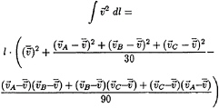
(13)
2.3
Test Cases
Test cases concerned a sphere and two ships. The HSVA tanker, used often as a test for RANSE flow codes, has a ‘parabolical' bow shape and a much finer afterbody, thus showing the strong asymmetry in x direction which makes it well-suited to compare the numerically computed resistance in double-body
flow conditions with the correct value of 0. For comparison, Jensen 's “sphere method” [12] and a first-oder Hess&Smith panel method were applied (Table II ). The patch method was more accurate by one order of magnitude for the same discretisation (corresponding roughly to same CPU time and storage requirements for the 3 methods).
Table II. Numerical resistance coefficient –2Fx/ρU2S by different methods
|
method |
no. of panels/patches |
1000 · resistance coefficient |
|
Patch Sphere |
421 421 |
–0.16 +1.54 |
|
Patch Sphere |
780 780 |
+0.03 +0.20 |
|
Hess&Smith |
1788 |
+0.20 |
Table III shows a comparison of the force on 1/8 of a full sphere in uniform flow. For radius 1 and speed 1, the exact force components on the positive octant are fx=–π/64=0.04909 and fy=fz=11π/128=0.26998. Here the patch method was compared by Hughes and Bertram [3] with an ordinary higher-order panel method OHM (parabolic in shape, linear in source strength). The patch method is roughly of same accuracy (but much faster) for the longitudinal force, but 3 times more inaccurate for the transverse force. Results of the patch method in Table III refer to a mesh of equilateral triangles; it was found, however, that combining two such triangles to a quadrilateral produced nearly the same error with about half the number of patches.
Table III: Error in force on 1/8 sphere
|
patch method PTM |
||
|
elements |
Fx error |
Fy error |
|
16 |
0.006 |
0.050 |
|
64 |
0.001 |
0.012 |
|
256 |
0.00005 |
0.0025 |
|
higher-order panel OHM |
||
|
elements |
Fx error |
Fy error |
|
15 |
0.006 |
0.017 |
|
66 |
0.002 |
0.004 |
|
231 |
0.0007 |
0.0013 |
Fig.3 shows the wave resistance coefficient for the Series 60–CB=0.6 hull as a function of Froude number, computed by a non-linear Rankine source/patch method. For the hull boundary condition up to the deformed water surface and for the force integration, the patch method was used,
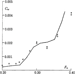
Fig. 3. Wave resistance coefficient of Series 60 (CB= 0.6) model according to experiments ([13], line) and patch method (○). Symbols ● include interaction with viscous resistance.
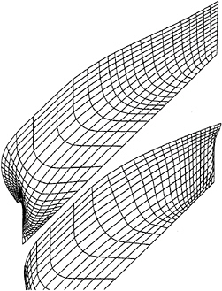
Fig. 4. Patch arrangement on Series 60 hull
whereas the free surface condition was satisfied, as in earlier methods, by point collocation and point sources above the water surface shifted backwards relative to the collocation points. Symbols • include a rough approximation of the interaction between wave and viscous resistance: the difference between • and ○ corresponds to the change of viscous resistance with Fn estimated to be proportional to the change of wetted surface and to the mean squared non-viscous velocity at the hull surface.
To test the accuracy of the patch method, the hull discretisation shown in Fig.4 with 37 · 13 patches was modified to have twice the number of patches, either in transverse or in longitudinal direction. The results of the wave resistance were practically the same for all three meshes.
3.
Cluster and Multigrid Method
3.1
Clustering
In the following only the boundary condition on the body (no flow through the hull) is considered; but clustering and the multigrid technique are even well applicable also for free-surface flow problems.
The discretisation of the hull boundary condition yields a system of linear equations for the unknown source strengths σi in (1):
Kσ=g (14)
K is the coefficient matrix, σ the vector of source strengths, and g the vector of the inhomogeneous parts. An element kij of K can be interpreted as flow through a patch i per time induced by a source of unit strength at point ![]() . The elements of g give the negative flow per time through the patches induced by the uniform flow. Eq. (14) enforces that the superposition of all source flows and the parallel flow add up to zero flow through all patches.
. The elements of g give the negative flow per time through the patches induced by the uniform flow. Eq. (14) enforces that the superposition of all source flows and the parallel flow add up to zero flow through all patches.
Clustering aims to reduce the computer time and storage requirements for generating the matrix K, and it simplifies the application of the multigrid method (next chapter); however, clustering and multigrid can be applied also separately. The cluster/multigrid technique is combined here with the patch method, but it could be applied also to ordinary panel methods.
Here, a cluster is a set of 4 by 4 patches of the normal (fine) grid. The 16 patches of each cluster are generated to have similar size and shape, and the surface covered by a cluster should be smooth; if it is not, the cluster should be made smaller.
The scalar equations in (14) referring to a line of four patches in a cluster are added and subtracted to the following four combined equations:

If the combined equations are satisfied, so are the original ones. The absolute values of coefficients of the combined equations 2, 3, and especially 4 decrease stronger with distance from the main diagonal in K than those of the original equations and of combination 1.
Correspondingly also the four rows of patches within a cluster are combined to the following 16 combinations of 16 equations:
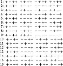
As the cluster consists of patches of approximately equal size and orientation, for a distant source the influence functions of all combinations will nearly cancel (due to the positive and negative contributions) with the exception of the first combination which adds all influence functions. The purpose of combining the influence of elements within a cluster is, that for large distances between source and patch (resp. collocation point and panel in a conventional panel method) the combined influence functions are so small that they can be neglected. This saves storage space, time for solving the system of equations and—if one can determine a priori which combinations will be neglected—time for computing the influence functions, because only the combined influence functions for all elements of a cluster or for 2 by 2 patch blocks need to be computed.
The mixed influence functions (containing positive and negative contributions) decay even more rapidly with distance as also sources within a source cluster of 16 sources are combined by adding and subtracting their influence. Contrary to patch clusters, however, experience has shown that it is not sufficiently accurate to use just one single point source to represent a whole source cluster even for large distances. Thus, forming source clusters reduces storage requirements, but not time to compute the coefficient matrix.
The matrix K is subdivided into blocks of 16 · 16=256 elements. Each block represents the influence of one source cluster on one patch cluster. A block element represents initially the influence function of a source of unit strength on one patch; if 4 or 16 patches are combined to save computation time, each patch of the group is assumed to have 1/4 resp. 1/16 of the computed total influence. Then the block elements are ‘mixed' according to the above combinations. A direct superposition of each of the 256 elements of a 'mixed' block by adding and substracting all elements of the original block would require 2 · 2562 arithmetical operations per block. Mixing can be accelerated by combining, stepwise, at first two adjacent elements, then more removed elements. An example of 4 elements may illustrate the process: Original coefficients (○ indicates that a neighbour coefficient does not contribute):
![]()
Neighbours added/subtracted:
![]()
Neighbours once removed added/subtracted:
++++ +–+– ++–– +––+
For 256 elements, this process requires only 2 · 256 · 8 operations. After ‘mixing', each of the 256 block elements represents the combined influence of 16 sources/sinks on the ± combination of 16 patches.
Five types of blocks are distinguished according to their arrangement of non-zero elements, Fig.5. The threshold for setting an element to zero was taken such that the error in neglecting all zero elements contributes less than 10–4U to the final velocity. The definition of block types was based on trial computations to achieve favourable storage and CPU time conditions; however, a higher number of block types may be worthwhile to further reduce the storage requirements. Each block of matrix K is stored without the zero elements in one storage area. The full matrices of type 1 appear mostly along the main diagonal, whereas the sparse blocks of higher block type are located farther away from the main diagonal, where large distances between patch and source group are represented.
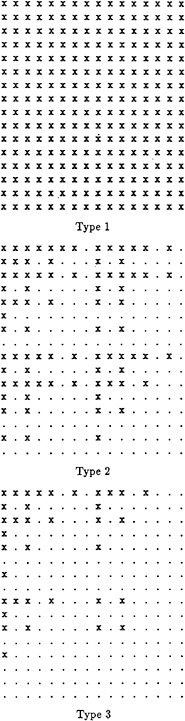
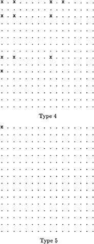
Fig. 5: Arrangement of non-zero elements (x) in five block types
3.2
Multigrid Method
The multigrid method is frequently used for solving differential equations of viscous fluid flow, but it works even better for potential flow problems, i.e. for solving integral equations. The principles of both applications are elaborated in [8]. For panel methods the multigrid technique reduces the time needed to solve the system of linear equations (14) to a negligible fraction of the total computing time.
First, the rows in K and g are multiplied by factors such that the elements of K on the main diagonal are all 1. Then a multigrid solution can be determined as follows: Starting from ![]() a Jakobi iteration step improves σ by smoothing the error in the system of equations on the normal (finest) grid:
a Jakobi iteration step improves σ by smoothing the error in the system of equations on the normal (finest) grid:
(15)
Index l indicates the grid level: l=3 denotes the finest grid in the investigated 3-grid method, l=1 the coarsest grid. Superscripts i denote the iteration step. I is the unit matrix, ![]() the improved vector of unknown source strengths.
the improved vector of unknown source strengths.
A straight-forward Jakobi iteration of (15) would take ![]() l as next iterative solution
l as next iterative solution ![]() . The multigrid method improves convergence by setting
. The multigrid method improves convergence by setting
(16)
The vector of residuals ![]() gives the error of all equations. This residual is restricted to a shorter vector, here to 1/4 of the original number of elements, by the restriction operator r explained later. Kl–1 is, correspondingly, a restricted coefficient matrix with 1/4 of the original columns and rows. Multiplication of the residuals with the inverse matrix
gives the error of all equations. This residual is restricted to a shorter vector, here to 1/4 of the original number of elements, by the restriction operator r explained later. Kl–1 is, correspondingly, a restricted coefficient matrix with 1/4 of the original columns and rows. Multiplication of the residuals with the inverse matrix ![]() yields the necessary corrections to enforce the equations exactly. Because we perform the corrections on a coarser grid, we have to transform them to the original, fine grid by applying the prolongation operator p (see later). The prolongated corrections added to the approximation
yields the necessary corrections to enforce the equations exactly. Because we perform the corrections on a coarser grid, we have to transform them to the original, fine grid by applying the prolongation operator p (see later). The prolongated corrections added to the approximation ![]() yield the next approximation
yield the next approximation ![]() . This is again used in (15) and improved by (16) until the residual is decreased by 5 to 6 orders of magnitude.
. This is again used in (15) and improved by (16) until the residual is decreased by 5 to 6 orders of magnitude.
To determine ![]() requires to solve a system of linear equations having 1/4 of the original number of unknowns. This system is also solved by applying the multigrid equations (15) and (16), now with l=2. There remains a system of 1/16 of the original number of unknowns, which is effectively solved by Gauss' algorithm.
requires to solve a system of linear equations having 1/4 of the original number of unknowns. This system is also solved by applying the multigrid equations (15) and (16), now with l=2. There remains a system of 1/16 of the original number of unknowns, which is effectively solved by Gauss' algorithm.
Combined with our clustering technique, the restriction and prolongation operators become extremely simple: For l=3, in each block of 16 vector components the restriction operator eliminates 12 components, keeping only the 1st, 3rd, 9th and 11th. That means: In (16) only the flow through 2 · 2 patch groups is considered, not the flow through single patches. The solution ![]() gives corrections of the source combinations 1, 3, 9, and 11, i.e. corrections of the combined source strength for groups of 2 · 2 sources. To this end, K2 is produced from K3 by keeping in each block of 16 · 16 elements only those in rows and columns no. 1, 3, 9 and 11. For prolongation, the additional elements, i.e. the corrections of the differences between single source strengths within a block of 2 · 2 sources, are simply set to zero; these differences are effectively corrected by the Jakobi step (15).
gives corrections of the source combinations 1, 3, 9, and 11, i.e. corrections of the combined source strength for groups of 2 · 2 sources. To this end, K2 is produced from K3 by keeping in each block of 16 · 16 elements only those in rows and columns no. 1, 3, 9 and 11. For prolongation, the additional elements, i.e. the corrections of the differences between single source strengths within a block of 2 · 2 sources, are simply set to zero; these differences are effectively corrected by the Jakobi step (15).
For l=2, the restriction operator keeps only the first element of each block of 4 elements, i.e. the combined flux through a 4 · 4 panel group, and the prolongation operator adds 4 zero elements in each group of 4 components. Matrix K1 contains the 1st, 5th…row and column of K2.
3.3
Test Case
As a test case, the double-body flow around a Wigley hull with 1600 patches (100 clusters) on one ship side was computed. This number of elements is more than necessary for this flow; it is used here only to demonstrate the effect of multigrid and clustering for the typical, larger panel numbers in practical applications. A full coefficient matrix would have required 16002=2.56 · 106 coefficients. Clustering reduced this to 0.35 · 106 (14%) coefficients. The additional storage space is negligible: For each of the 10000 storage blocks, block type and starting address in the coefficient array have to be stored.
On a 12 Mflop computer, the computing time was 73s for determining the coefficient matrix, 2.5s for solving and 33s for determining end results (velocities, pressures, forces). It was necessary to use double precision of the real variables; otherwise the multigrid method did not converge to sufficiently small residuals. A comparison with a coarser discretisation of the Wigley hull involving only 30 clusters (480 patches) showed that the storage requirement was ~ n1.25, the total computing time ~ n1.78. Only for systems with more than about 800 elements, the multigrid and clustering approach saved CPU time. However, storage savings are attained already for considerably smaller systems of equations.
4.
New Higher-Order Panel Method
The purpose of higher-order panels is to increase the accuracy for a given number of unknowns, and to determine spatial derivatives of flow velocities which—for decreasing grid spacing—converge to the correct values. The latter is necessary for seakeeping calculations with forward speed that linearise around the steady flow potential around the body [θ]. The usual higher-order panels following the original work of Hess [10] can compute the necessary velocity derivatives, but they failed to improve accuracy for real ship geometries in [3]. Furthermore they involve quite complicated formulas especially for higher derivatives of the potential.
The new higher-order panel method presented here varies the approach of Kouh and Ho [11]. Both methods are based on a modification of the integrals which give the influence of a source (in my method: and dipole) distribution on the body surface, such that the integrand is non-singular even if the field point is on the body surface, too. This allows to substitute the complicated analytical integration of the singular integrand by a simple numerical scheme.
Differently from [11] and from eq. (1), the ‘direct' method is used here. It applies a distribution of sources and dipoles on the body surface and solves directly for the potential at many points on the body surface. Comparisons seemed to indicate that for non-lifting flows (without circulation and without a Kutta condition) both the direct and the indirect method are about even well suited, whereas for lifting flows the direct method is superior in accuracy to the indirect method, which—for lifting flows—uses also sources and line vortices (corresponding to dipole panels).
The well-known equation for the direct (source-dipole) panel method is
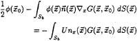
(17)
with the Green function
(18)
![]() =disturbance potential,
=disturbance potential, ![]() =unit normal vector on the closed surface Sb, U=ship speed and
=unit normal vector on the closed surface Sb, U=ship speed and ![]() =a field point on Sb. The integrals in (17) are desingularised (without moving the singularities into the interior of
=a field point on Sb. The integrals in (17) are desingularised (without moving the singularities into the interior of
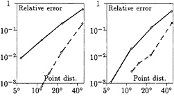
Fig. 6. Relative error of transverse (left) and longitudinal (right) pressure force on 1/8 of a sphere for patch (continuous) and higher-order method (broken line)
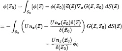
(19)
![]() 0 is the constant potential generated by the source distribution δ in the space surrounded by Sb, i.e. inside the body. δ is the ‘eigen potential' following from the homogeneous integral equation
0 is the constant potential generated by the source distribution δ in the space surrounded by Sb, i.e. inside the body. δ is the ‘eigen potential' following from the homogeneous integral equation
(20)
Eq. (20) has a solution δ which has non-zero values everywhere on Sb. Eq. (20) is also desingularised:
(21)
The nonsingular integrals in (21) and (19) are evaluated by Simpson 's rule using 9-knot panels (8 on the circumference, one in the center), to obtain a system of linear algebraic equations for the potential at each knot. Numerical interpolation and differentiation over the panels gives velocities, velocity derivatives, and pressures on Sb.
For a sphere in uniform flow, Fig.6 compares relative errors of the pressure force on 1/8 sphere between the higher-order and the patch method. For both methods, the mesh consisted of quadrilaterals bounded by meridians and latitude circles with uniform angular spacing, poles being at the stagnation points. (Results for the patch method given in Fig.6 differ somewhat from Table III because there a mesh of nearly uniform, equilateral triangles was used.) The higher-order method is, roughly, 10 times more accurate than the patch method which is again much more accurate than an ordinary first-order panel method. For more complicated bodies, however, the difference is expected to be much smaller. Both the maximum error in ![]() (not shown) and the pressure force (Fig.6) converge with errors ~ h3.5 to h4, where h is the grid spacing.
(not shown) and the pressure force (Fig.6) converge with errors ~ h3.5 to h4, where h is the grid spacing.
References
1. Bertram, V., “Numerische Schiffshydro-dynamik in der Praxis”, rep. 545, 1994, Inst. für Schiffbau, Hamburg Univ., Germany
2. Bertram, V.; Jensen, G., “Recent applications of computational fluid dynamics”, Ship Techn. Res. 41/3, 1994, pp. 131–134
3. Hughes, M.; Bertram, V., “A higher-order panel method for 3-d free surface flows”, rep. 558, 1995, Inst. für Schiffbau, Hamburg Univ., Germany
4. Zou, Z.; Söding, H., “A panel method for lifting potential flows around a yawed ship in shallow water”, 20th Symp. on Ship Hydrodyn., 1994, Santa Barbara
5. Zou, Z., “Calculation of the three-dimensional free-surface flow about a yawed ship in shallow water”, Ship Techn. Res. 42/1, 1995, pp. 45–52
6. Bertram, V.; Yasukawa, H., “Rankine source methods for seakeeping problems”, Proc. Schiffbautechn. Gesellschaft, Springer, Berlin, Heidelberg, New York, Tokyo, 1996
7. Söding, H., “A method for accurate force calculations in potential flow”, Ship Techn. Res. 40/3, 1993, pp. 176–186
8. Hackbusch, W., Multi-grid methods and applications , Springer, Berlin, Heidelberg, New York, Tokyo, 1980
9. Bertram, V., “Ship motions by a Rankine source method”, Ship Techn. Res. 37/4, 1990, pp. 143–152
10. Hess, J.L., “A higher order panel method for three-dimensional potential flow”, NADV-Report, MDC J8519, 1979
11. Kouh, J.S.; Ho, C.H., “A high order panel method based on source distribution and Gaussian quadrature”, Ship Techn. Res. 43/1, 1996, pp. 38–47
12. Jensen, G.; Söding, H., “Ship wave-resistance computations”, Notes on Num. Fluid Mech. Vol. 25: “Finite approximations in fluid mechanics”, Springer, Berlin, Heidelberg, New York, Tokyo, 1989
13. Kajitani, H., “A wandering in some resistance components and flow”, Ship Techn. Res. 34/3, 1987, pp. 105–131
DISCUSSION
W.W.Schultz
University of Michigan, USA
The patch method results are impressive. Is this improvement due primarily to moving the singularity distribution within the body or is the matching of the outflow through the patch also required? Specifically since (3) appears to ensure Σσi=O inside the closed body, is the extra effort in evaluating the trigonometric functions worth it?
Does the higher-order method you present make the patch method obsolete? Why would you still use the patch method?
AUTHOR'S REPLY
The improvement in the patch method is not due to moving the singularities into the body, but due to “averaging” both the boundary condition and the results (e.g., the pressure) over each patch. Moving the singularity into the body would be helpful, but is possible only if the body surface is sufficiently smooth and if the body breadth is sufficient; these conditions are not satisfied at typical ships' ends. The extra effort for computing trigonometric functions appears only in comparison with a point-source-point-collocation method, which does not work well for typical ships; compared to a usual first-order panel method the numerical effort per panel/patch is about the same.
The higher-order method is more accurate for smooth bodies, but somewhat more complex to program. Comparisons for less smooth bodies like ships with sharp ends have not yet been made. Extension to free-surface flows may further change the rating.


