
4
Effects of Automotive Technology, Energy, and Regulatory Developments on Finance
Important policy initiatives of the federal and some state governments have the goal of reducing oil use in order to reduce dependence on foreign oil suppliers and emissions of greenhouse gases and other pollutants. This chapter examines the extent to which revenue from highway user fees might diminish over time as the result of these policies. Reduced oil consumption will reduce revenues if tax rates are not raised to compensate. Transportation officials’ apprehension in this regard is understandable in light of the history of tax rates and revenues described in Chapter 2. Rapid improvement in fuel economy and higher fuel prices were among the factors that contributed to the pronounced decline in constant-dollar highway user fee revenue and highway spending in the 1970s and early 1980s, until legislatures responded with rate increases.
This chapter examines the likelihood that rising fuel prices, new automotive technology, or new environmental and energy regulations will affect revenues from highway user fees in the next two decades. If large improvements in fuel economy or transition of the highway fleet to new energy sources appears likely within this period, planning for adjustment or replacement of the present fuel-tax-based finance system will be needed to avoid unintended declines in revenue. The first two sections below review projections of world petroleum supply, consumption, and price and of motor vehicle technology and fuel consumption in the United States. The third section considers possible U.S. regulatory developments that may affect fuel consumption and fuel tax revenue.
SUPPLY, PRICE, AND CONSUMPTION OF PETROLEUM FUELS
The future path of motor fuel prices will affect the revenues derived from established user fees because fuel prices influence travel volume, fuel economy, and the types of fuels used. Through its effect on travel volume, the price of fuel also will influence the cost of providing roads.
This section presents historical and projected price and consumption trends primarily from U.S. Department of Energy (DOE) sources: the Annual EnergyOutlook 2005 (EIA 2005a), Annual Energy Outlook 2006 Early Release (EIA 2005b), and Future U.S. Highway Energy Use: A Fifty Year Perspective (Birky et al. 2001). Each edition of the Annual Energy Outlook (AEO) is a 25-year projection of energy supply and consumption produced by DOE on the basis of its National Energy Modeling System and System for the Analysis of Global Energy Markets. Highway Energy Use is a more qualitative analysis of possible future developments in petroleum and fuels markets, highway use, and motor vehicle technology.
The AEO 2006 Early Release reference case projections show a slight increase in the U.S. retail gasoline price from its 2004 average of $1.90 per gallon to $2.13 in 2025 (in 2004 dollars) (Table 4-1, Figure 4-1). Comparison of this projection with DOE’s 2005 and 2004 AEOs illustrates the current great uncertainty in oil market projections after 3 years of sharp price increases. DOE’s 2006 reference case world oil price projection for 2025 ($48 per barrel) is 54 percent above the corresponding projection in the 2005 AEO ($31 per barrel in 2004 dollars) and the 2025 gasoline price is 31 percent higher (Table 4-1). The 2006 AEO reference case projections and assumptions are similar to the 2005 edition’s “High B” world oil price case, the highest price scenario presented in that edition. DOE explains the changes as follows: “In preparing AEO2006, EIA reevaluated its prior expectations about world oil prices in light of the current circumstances in oil markets. Since 2000, world oil prices have risen sharply as supply has tightened, first as a result of strong demand growth in developing economies such as China and later as a result of supply constraints resulting from disruptions and inadequate investment to meet demand growth…. In the AEO2006 reference case, the combined production capacity of members of the Organization of Petroleum Exporting Countries (OPEC) does not increase as much as previously projected, and consequently world oil supplies are assumed to remain tight” (EIA 2005b, 2, 4).
In the 2005 AEO edition, DOE had already raised its 2025 gasoline price projection by 12 percent in the reference case, compared with the 2004 edition, and by 37 percent in the highest world oil price projection presented. None of the AEO cases is intended to reflect consequences of petroleum supply disruptions.
DOE predicts that producers will be able to expand world oil output by nearly 40 percent and U.S. motorists will be able to increase travel by nearly 50 percent from 2003 to 2025 while the price of gasoline is maintained near $2.00 per gallon. The gasoline price will increase more slowly than the world oil price because
TABLE 4-1 Projected Growth Rates of World Oil Production, Oil and Gasoline Price, U.S. Motor Vehicle Travel, and Fuel Consumption (EIA 2005a, Tables D3, D4, D7; EIA 2005b, Tables A1, A7, A12)
|
|
AEO 2005 |
AEO 2006 |
||||
|
Reference Case |
High B Price Case |
Reference Case |
||||
|
2003–2025 Increase (%) |
Annual Rate (%) |
2003–2025 Increase (%) |
Annual Rate (%) |
2003–2025 Increase (%) |
Annual Rate (%) |
|
|
Gasoline price |
−1 |
0.0 |
26 |
1.0 |
29 |
1.2 |
|
World oil price |
9 |
0.4 |
73 |
2.5 |
69 |
2.4 |
|
Annual world oil production |
51 |
1.9 |
41 |
1.6 |
39 |
1.5 |
|
Annual U.S. vehicle miles |
57 |
2.1 |
51 |
1.9 |
48 |
1.8 |
|
Annual U.S. highway motor fuel consumption |
51 |
1.9 |
42 |
1.6 |
39 |
1.5 |
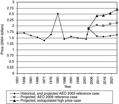
FIGURE 4-1 Gasoline prices, historical and projected, 2004–2025. (Sources: EIA 2005a, Table A12; EIA 2005b, Table A12; EIA 2005c, Table 5.24. Price deflator: BEA 2005, 48, 188, 189.)
the gasoline price includes refining and distribution costs and taxes. (DOE’s gasoline price projections appear about equal to the price of the raw material plus $1 per gallon for refining, distribution, and tax.)
To suggest a range of possible future prices, Figure 4-1 shows the historical gasoline price and three projections: the AEO 2006 Early Release reference case (the only case presented in the Early Release), the AEO 2005 reference case as a low projection, and a high case constructed by multiplying the 2006 AEO reference case price by the ratio of the price in the 2005 AEO High B case to the 2005 AEO reference case price in each year. The 2025 price in this upper bound case is $2.70 per gallon, corresponding to an oil price of about $75 per barrel. (DOE points out that the oil prices in its tables until the 2006 AEO were “average refiner acquisition cost” for imported crude and that this price has typically been several dollars per barrel less than the prices of premium low-sulfur crude, which are usually reported in news stories. In the 2006 AEO, DOE has begun highlighting the premium crude prices. This chapter refers only to the average refiner acquisition cost. The $48 per barrel average refiner acquisition price projected for 2025 in the 2006 AEO corresponds to $54 per barrel for imported low-sulfur light crude.)
DOE calls its world oil price projections scenarios; that is, they are assumptions that are consistent with the available facts. Because the price of oil has been erratic in recent decades and is strongly affected by diverse political, economic, and technological factors, oil price forecasts have not been very successful. For example, the 1995 AEO projection for 2005 was $22 per barrel in the reference case and $39 per barrel (in 2005 dollars) in the high oil price case. The actual 2005 price was about $50, although the actual price during 1995–2005 usually was between the 1995 AEO reference and high projections. DOE compared its AEO 2005 projections with nine other published projections or scenarios and observed that the range between the 2005 AEO Low and High B cases spanned the range of published projections. In 2025, the range of projections reviewed was $24 to $37 per barrel (in 2003 dollars), compared with DOE’s projected range of $21 to $48 per barrel (EIA 2005a, 114–115). Probably the most useful aspect of the AEO projections and other projections described below is their qualitative assessments of critical underlying factors that will influence the price of oil. In the projections the committee reviewed, the critical factors identified are that (a) supplies are available from multiple sources that can be developed and brought to market at lower cost than the 2005 price and (b) sustaining the price at too high a level would not be in the interest of producers because it would stimulate enough conservation and production from alternative sources to lower their incomes. The projections take into account rapid growth in oil consumption in China, India, and some other developing economies. For example, in DOE’s 2006 reference case projection, oil consumption in China grows at over twice the world rate and China’s share of world oil consumption increases from 8 percent in 2004 to 12 percent in 2025 (EIA 2005b, Table A20).
A review (Gately 2001; Gately 2004) of the DOE 2001 and 2002 projections (similar in method to the projections through AEO 2005) and of two other prominent forecasts (from the International Energy Agency’s World Energy Outlook2000 and in the 2001 British study, The New Economy of Oil, by J. Mitchell et al.) with parallel results concluded that all were based on certain implausible assumptions. In particular, the projections were not derived from a behavioral model of the OPEC nations’ production decisions. Instead, OPEC oil production was projected as the residual between projected demand and non-OPEC production, given an assumed price path.
Simulations presented in the review articles indicate that if OPEC is moderately effective in controlling output in its own interests and oil price increases are as moderate as DOE projected (before AEO 2006), then demand must be more responsive to price than it is in the DOE projections. The author argues that maintenance of cartel pricing will be easier in the future, in part because expanding production from OPEC oil fields will require substantial investment to develop new capacity, whereas in recent decades capacity was in excess and output could be expanded with little effort. The simulations start with ranges of assumed rates of
OPEC’s target production growth (between 1 and 4 percent annually) or target market share (from 32 to 52 percent of world production; today’s share is 37 percent) and use plausible ranges of elasticities and non-OPEC production costs. In the results, OPEC’s revenue is not very sensitive to its rate of output expansion. The simulations indicate a likely oil price range of $24 to $36 per barrel (2000 dollars) in 2020 (Gately 2001, Figure 7; Gately 2004, Table 3), which is hardly different from most of DOE’s projections before AEO 2006, but these prices correspond to lower OPEC production than DOE projected. The implication of this analysis is that the current price and DOE’s latest projections are above the price that is in the long-term interest of the major producers. As DOE emphasizes in AEO 2006, a major source of supply and price uncertainty will be the willingness of producing nations to undertake investments in capacity expansion.
The DOE study Future U.S. Highway Energy Use (Birky et al. 2001) discusses some of the technological factors underlying projections of supply and demand elasticities. Although the report begins with disquieting observations about depletion of petroleum reserves, it concludes that petroleum supply developments, acting solely through the market, are unlikely to have decisive impact on U.S. automotive technology or travel behavior in the next several decades.
A figure in the report captioned “The World Oil Gap” shows a peak in “conventional” oil production in 2020 and a growing gap between conventional production and the extrapolated demand trend afterwards (Figure 4-2). The report observes: “The gap between continuing demand growth and declining production could be around 50 billion barrels of oil equivalent … by 2050, or almost twice current conventional oil production” (Birky et al. 2001, 3). Projections of the date
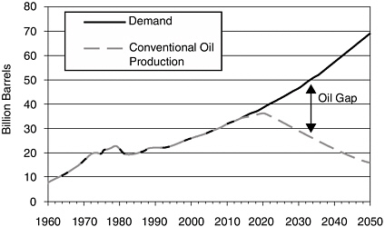
FIGURE 4-2 The world oil gap. (Source: Birky et al. 2001.)
of peak conventional oil production have received considerable exposure, for example, in the 1998 Scientific American article “The End of Cheap Oil,” which predicted peak world conventional oil production before 2010 (Campbell and Laherrère 1998). Such predictions are derived by projecting future reserves and assuming continuation of historical relationships of reserves to production. Earlier applications of the method proved to be overly pessimistic. Projections from the 1970s were summarized in a 1979 study (Brown et al. 1979, 27):
There are of course, basic physical constraints that will ultimately determine the level of world oil production. Projections based largely on these constraints—the reserves-to-production ratio in particular—indicate that production can increase somewhat further before peaking around 1990. [A 1979 U.S. Geological Survey study] consider[s] these ultimate production limits: “Extrapolation of historical trends in exploitation and production, together with an estimate of the stock of oil in known fields, and the assumption that the crude oil reserve-to-production ratio never drops below 10, places the date of peak world oil production before the end of 1993.” And an early 1979 study by the International Energy Agency concludes “that world oil production is likely to level off sometime between 1985 and 1995.”
In reality, conventional oil production expanded throughout this period (Figure 4-2).
As Future U.S. Highway Energy Use acknowledges, when conventional production does begin to decline, there are strong grounds for believing that the market will be capable of providing for the transition to unconventional sources without supply disruptions or any dramatic discontinuity in price. Unconventional resources that may be processed to produce liquid fuels include tar sands, oil shale, heavy oil, natural gas, and coal (Birky et al. 2001, ES-1). Supplies of unconventional resources are enormous, and production costs for some sources are less than the present world price of oil [e.g., according to the financial reports of one producer, its 2004 average operating costs (including interest, depreciation, and depletion) were CA$19.40 per barrel, or US$16.50 (Canadian Oil Sands Trust 2005, 2, 26)], although the mining and processing operations required to exploit some resources would face significant environmental constraints. DOE’s International Energy Outlook predicts gradual development of “nonconventional production” over the next two decades, increasing from 2 percent of world oil production in 2001 to 5 percent in 2025 in the reference case and 9 percent in the high oil price case (EIA 2005d, 160–161).
Extensive development of unconventional oil resources would open the way to consumption of high-carbon fuels for the indefinite future, well after conventional oil supplies were exhausted. Therefore, policies aimed at controlling greenhouse gas emissions may eventually block or supersede development of these resources (Grubb 1998).
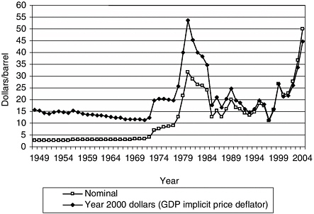
FIGURE 4-3 Crude oil domestic first purchase prices, 1949–2005. Point for 2005 is June price. (Sources: EIA 2004a, Table 5.18; EIA 2004b, Table 1; EIA 2005e, Table 9.4.)
The history of oil prices since the energy crisis of the 1970s has been volatile (Figure 4-3). None of the projections reviewed explicitly considers the impact of more volatile prices on future fuel economy. Even if the long-run track of average oil price follows a moderate path, more frequent and extreme price spikes in the future may stimulate purchases of high-mpg or alternative-fuel vehicles, although the historical evidence suggests that the magnitude of this effect may not be great.
MOTOR VEHICLE TECHNOLOGY PROJECTIONS AND FUEL TAX REVENUE
Because of the importance of the fuel tax in financing highway programs, highway agencies are interested in projections of fuel economy and motor vehicle technological developments. Improvement in fuel economy would create pressure for the federal government and the states to raise fuel tax rates or curtail highway spending. In addition, in the absence of changes in the user fee system, expansion of use of vehicles that do not consume taxed liquid fuels (e.g., battery-powered electric vehicles) would reduce revenues, and the states anticipate that lawmakers will consider promoting introduction of alternative fuels and technology through highway user tax breaks such as the break gasohol received until 2005. As an aid in assess-
ing whether these concerns are warranted, this section summarizes technology projections from five sources:
-
DOE’s Annual Energy Outlook (EIA 2005a; EIA 2005b)—the reference case and the high technology case from AEO 2005 and the reference case from the AEO 2006 Early Release. The fuel economy improvement by 2025 in the AEO 2006 reference case [with 2025 gasoline price at $2.13 per gallon (in 2004 dollars) compared with $1.63 per gallon in the earlier edition] is similar to the improvement in the high technology case of AEO 2005. The three cases are presented to indicate the sensitivity of DOE’s mpg projections to fuel price and technology assumptions.
-
A 2002 National Research Council (NRC) study of feasibility and costs of improvements in fuel economy for various classes of vehicles (NRC 2002).
-
A National Cooperative Highway Research Program (NCHRP) study that projected the effect of possible future fuel economy improvements and increased use of alternative fuels on Federal Highway Trust Fund revenue (Cambridge Systematics 2003).
-
A California Air Resources Board (CARB) analysis supporting its proposal for regulations requiring reductions in carbon dioxide emissions by vehicles sold in California beginning in 2009 (CARB 2004).
-
The DOE Future U.S. Highway Energy Use study described above (Birky et al. 2001).
These studies are described in Appendix B, along with two other studies of future automotive energy efficiency: a report on global automotive energy consumption of the Sustainable Mobility Project by the World Business Council for Sustainable Development (SMP 2004) and a 2004 NRC study of prospects for hydrogen-fueled vehicles (NRC 2004).
Table 4-2 shows fuel economy projections or scenarios from the five studies. With the exception of the AEO reference cases, the projected fuel efficiencies are not technology forecasts. Rather, they specify technology exogenously, consistent with stated criteria relating to cost, vehicle performance requirements, and technological feasibility. The mpg values are the researchers’ estimates of fuel economy improvements that might reasonably be expected as the consequence of new regulations or increases in the price of fuel.
The NRC and CARB scenarios are intended to represent fuel economy improvements that would be cost-free to drivers: they would not involve general downsizing of vehicles or degrade performance, and the capital and operating costs of the technology improvements would be paid for by fuel savings. Such assessments of feasibility are controversial. For example, the motor vehicle industry claims that the initial cost of the CARB projected technology package to new car
TABLE 4-2 Automotive Technology Projections and Scenarios
|
Source |
Assumptions |
Projection Year |
Projected ldv mpg |
Percent Reduction in gpm Versus 2003f |
|||
|
New Vehicle: EPA |
New Vehicle: On-Roada |
Fleet |
New Vehicle |
Fleet |
|||
|
DOE AEO 2006 Early Release reference case |
Greater sales of hybrid and diesel vehicles than in 2005 reference case (14% of 2025 sales). |
2025 |
28.8 |
25.0 |
22.0 |
13 |
9 |
|
DOE AEO 2005 reference case |
19% of ldv sales in 2025 are advanced technology (including HEV) or alternative fuels. 80% of advanced technology sales are result of regulation. 2025 new car hp 26% above 2003. |
2025 |
26.9 |
23.4 |
21.0 |
7 |
5 |
|
DOE AEO 2005 high-technology case |
Lower cost, greater efficiency gains, and earlier introduction for advanced technology than in reference case. |
2025 |
28.8 |
25.0 |
22.1 |
13 |
10 |
|
NRC 2002 average case |
Technologies adopted would yield fuel savings covering purchase price for constant vehicle size and performance and could be in production by 2015.b |
2015 |
29.8 |
25.9 |
|
16 |
|
|
NRC 2002 low-cost/high-mpg case |
As in average case, but optimistic assumptions regarding cost and effectiveness of technological improvements.b |
2015 |
32.1 |
27.9 |
|
22 |
|
|
NRC 2002 high-cost/low-mpg case |
As in average case, but pessimistic assumptions.b |
2015 |
27.4 |
23.8 |
|
8 |
|
|
NCHRP (Cambridge Systematics 2003) |
NRC 2002 fuel economy projections become regulatory requirements in 2015; phase-in starts 2006; vmt by size class and model year projections as in AEO 2002 reference case.c |
2020 |
|
|
23.2 |
|
14 |
|
CARB 2004 |
Technologies adopted would yield fuel savings covering purchase price for constant vehicle size and performance and could be phased into production between 2009 and 2014. |
2020 |
|
|
23.4 |
28 |
15 |
|
CARB 2004 |
As above. |
2030 |
|
|
26.4 |
28 |
24 |
|
Birky et al. 2001 enhanced conventional vehicles strategy |
Conventional IC engines with incremental technology improvements—weight reduction, engine/transmission enhancements, aerodynamics—as might be driven by high fuel prices.d |
2050 |
33.7 |
29.3 |
|
26 |
|
|
Birky et al. 2001 HEV/FCV hydrogen strategy |
New vehicle market 70% hybrid electric, 30% hydrogen fuel cell by 2040.d,e |
2050 |
41.0 |
35.6 |
35.6 |
39 |
44 () |
|
a On-road mpg is calculated as (EPA mpg)/1.15, on the basis of the approximate conversion factor reported in NRC 2002, Table 4-1. b The study reports mpg projections by vehicle size class, but not for the vehicle fleet. The fleet averages shown in the table are the average of the size class projections weighted by model year 2004 estimated market shares by size class from NHTSA 2003. c The study reports projected fuel consumption rather than mpg. The mpg values in the table are derived from projections of fuel consumption and vmt. d The study reports percentage changes in mpg but does not state the base year mpg. Mpg values in the table assume base year mpg values are values for 2000 in AEO 2002. e This scenario involves hydrogen fuel cell vehicles. The mpg values in the table are the values that would produce the equivalent reduction in fuel energy consumption in a liquid fuel–powered fleet. f Percentage reductions are with respect to 2003 U.S. average light-duty vehicle fuel economy according to AEO 2005: 20.0 mpg fleet, 25.1 mpg new vehicle EPA. Abbreviations: ldv: light-duty vehicle mpg: miles per gallon gpm: gallons per mile HEV: hybrid electric vehicle FCV: fuel cell vehicle IC: internal combustion DOE: Department of Energy NRC: National Research Council AEO: Annual Energy Outlook vmt: vehicle miles traveled |
buyers would be three times the state’s estimate (Hall 2004). The higher the cost (in vehicle purchase price or performance degradation) to motor vehicle owners, the less demanding regulatory efficiency standards are likely to be.
Taken together, the projections suggest that fuel economy improvements of 15 to 25 percent (i.e., an average decrease of 15 to 25 percent in fuel consumption per mile) for new light-duty vehicles would be practical within the next 10 to 20 years, without the need for technical breakthroughs and without downsizing or vehicle price increases that would seriously affect the vehicle market or driving habits. If such new-vehicle efficiency improvements were attained, the improvement in light-duty vehicle fleet fuel economy would be 10 to 20 percent by 2025, according to the projections. As noted, these are not projections of likely outcomes, but rather of fuel economy gains that could reasonably be expected if forced by regulation or fuel prices.
None of the projections foresees important use of vehicles not powered by gasoline, diesel, or ethanol blends before 2025. For example, they do not project significant market shares for hydrogen-fueled cars or electric vehicles with batteries charged from electric power lines. Thus, vehicles foreseen to be in use in 2025 will be subject to existing fuel taxes.
The three studies reviewed that consider the connection between fuel price and the motor vehicle market (EIA2005a, 62; SMP 2004, 104–105; Birky et al. 2001, 9) all conclude that no likely fuel price increase or technology development in the period to 2025 will have a dramatic market effect on fleet average fuel economy by 2025. (The NRC, CARB, and Birky et al. projections and scenarios summarized in Table 4-2 are assessments of possible improvements in fuel economy based on the assumption that the regulatory or market forces required to induce them are present; they are not forecasts of likely outcomes.) This is partly because present regulations elevated fuel economy above the level that would have prevailed at historical fuel prices in an unregulated market. In addition, during periods of stable fuel prices, consumers have shown a preference for taking advantage of efficiency improvement technology by buying larger, higher-performance vehicles rather than by reducing their dollars-per-mile operating costs. The implication of the projections in these three studies is that if fundamental changes in fuel economy, fuel price, or engine technology occur in the next several decades, they are more likely to be the result of government intervention than energy market developments.
After 2025, projections are essentially speculative, but if the rate of fuel economy improvement projected to 2025 in the AEO 2006 reference case were to continue for another 20 years, light-duty vehicle fleet fuel economy would be 24.5 mpg (an 18 per cent reduction in fuel consumption per mile compared with today). This fleet fuel economy is not inconsistent with the projection in the Enhanced Conventional Vehicles scenario in Future U.S. Highway Energy Use of new vehicle EPA fuel economy rating of 33.7 mpg in 2050 (equivalent to
new-vehicle on-road fuel economy of about 29.3 mpg) (see Table 4-2). According to the HEV/FCV (hybrid electric vehicle/fuel cell vehicle) Hydrogen scenario in Future U.S. Highway Energy Use, a complete conversion of new vehicle sales to a mix of hybrid electric vehicles and vehicles powered by fuel cells consuming hydrogen could occur by 2040. In this scenario, vehicle energy consumption per mile would be reduced by more than half by 2050 compared with today, and the reduction in consumption of traditional liquid fuels would be even greater (see the last line in Table 4-2). Hybrid electric vehicles combine an internal combustion engine with an electric motor powered by batteries (charged by the internal combustion engine or by energy captured during braking) in order to gain energy efficiency. A fuel cell is a kind of battery that consumes hydrogen or another fuel to produce an electric current (without combustion or a mechanical generator). The current powers an electric motor that propels the vehicle.
Truck Fuel Economy Trends
Twenty-three percent of all federal and state fuel tax revenue is from taxes on diesel fuel, nearly all of which is consumed by large, freight-carrying trucks (FHWA 2003b, Tables MF-121T, MF-27). Therefore, truck fuel economy trends are important for transportation program revenue. Large trucks have made substantial fuel economy gains in recent decades, but more stringent emissions regulations may retard future fuel economy improvements (DOE 2003). The 2006 AEO reference case projects a 9 percent reduction in fuel consumption per mile for the freight truck fleet by 2025 (to 6.6 mpg, from 6.0 in 2003) (EIA 2005b). The 2005 AEO also projected a 9 percent reduction in the reference case and a 10 percent reduction in fuel consumption per mile in the high technology case (EIA 2005a, Table A.7, p. 86).
Freight truck shares of highway vehicle miles and highway fuel consumption in 2003 and the AEO 2006 projections of 2025 shares are as follows:
|
|
2003 |
2025 |
|
Share of vehicle miles (percent) |
7.5 |
8.6 |
|
Share of fuel consumption (energy units, percent) |
21.2 |
23.4 |
DOE projects that annual vehicle miles of freight truck travel will grow 70 percent over the period. Freight trucks’ share of fuel consumed is projected to grow more slowly then their share of travel because projected fuel economy improvements are greater than for light-duty vehicles. If these projections are realized, trucking’s contribution to user fee revenues relative to its share of travel will decline unless legislatures make larger adjustments in truck tax rates than in rates affecting light vehicles.
Fuel Tax Revenue Implications
Developments in motor vehicle fuel economy and propulsion technology could affect the viability of the present transportation finance scheme in three ways. First, maintaining constant revenue per vehicle mile would require raising cents-per-gallonfuel tax rates if average fuel economy improves. Second, some technologies (e.g., electric and hydrogen-powered vehicles) do not consume the fuels that are now within the highway user tax scheme. Finally, lawmakers may decide to provide incentives for adoption of new technologies in the form of lower user fee payments (for example, the lower federal excise tax rate paid on gasohol than on gasoline before 2005).
The projections of fleet fuel economy percentage improvement in the last column of Table 4-2 indicate the magnitude of fuel tax rate increases that would be necessary to compensate for fuel economy improvements. Maintaining constant revenue per vehicle mile is a reasonable benchmark for judging fiscal impact, since, as Figure 2-1 shows, revenue has been fairly constant at around $0.035 per mile for the past 25 years. Maintaining constant revenue per vehicle mile after a 15 percent reduction in the fleet average fuel consumption per mile (i.e., a midpoint projection for 2025 from among the various optimistic technology scenarios summarized in Table 4-2) would require a 17.6 percent [100(0.15/0.85)] increase in the constant-dollar fuel excise tax rate. With such an increase, the 2003 combined federal and state tax rate on gasoline of $0.375 per gallon would rise to $0.441 per gallon. The fuel tax produces about 65 percent of all highway user revenues (see Table 2-2), about equal to half of all highway spending, so the revenue loss from an uncompensated 15 percent fuel economy improvement (assuming travel and vehicle sales were unaffected) would equal 10 percent of prior user fee revenues and 8 percent of spending.
The NCHRP study (Cambridge Systematics 2003) projected the effect on trust fund revenues of a range of alternative future tightenings of federal new-vehicle fuel economy standards, from a modest increase in the required fuel economy of new light trucks to a 50 percent increase in the required mpg for all vehicle classes compared with present legal standards. The projections were constructed to be consistent with the DOE AEO projections of travel by vehicle size class. In all cases, new-vehicle fuel economy standards are assumed to ramp up linearly from their present values in 2006 to their maximum values in 2015. One case assumes that the new standards are based on the estimates in the 2002 NRC study of cost-efficient improvements in fuel economy for each class of light-duty vehicle. (Table 4-2 shows the projected average new-vehicle fuel economy from the NRC study and the NCHRP study’s estimated fleet fuel economy.) The NCHRP authors argue that the NRC estimates or similar ones would be the most reasonable guide available to Congress if it were to decide soon to enact new fuel economy standards. The authors project that imposition of these standards would reduce light-duty vehicle fuel consumption by 9 percent in 2020 compared
with the AEO 2004 reference case and that Federal Highway Trust Fund revenue in 2020 would be reduced by $3 billion (7 percent). The federal revenue reduction in 2020 could be avoided by a $0.0125-per-gallon increase (in 2002 dollars) in the federal fuel tax.
The NCHRP study does not project revenues beyond 2020. The impact in later years would be greater, since the turnover of the fleet to higher-efficiency vehicles would not be complete in 2020. When turnover was complete (by 2025 or 2030), the revenue impact would be around 14 percent of trust fund revenues compared with revenues under the assumptions of the AEO reference case.
The NCHRP study also projects the revenue impact of continuation of the pre-2005 federal gasohol tax policy and of hypothetical additional federal measures to promote gasohol. Legislation enacted in 2004 raised the gasohol excise tax rate to equal the gasoline rate and provided that all revenue from the tax be credited to the Highway Trust Fund. This eliminated the prior trust fund revenue loss. However, the NCHRP study’s projections illustrate how pollution abatement and conservation incentives could have an important effect on user fee revenue. As Chapter 2 noted, if the federal excise tax on gasohol had been the same as for gasoline and credited to the trust fund, trust fund revenue would have been about $1.6 billion per year greater in 2002. Gasohol consumption was 21 billion gallons in 2002, 12.5 percent of all highway motor fuel use (FHWA 2003b, Tables MF-21, MF-33E). The NCHRP study considered the impact of legislation, proposed in Congress in 2003 but not enacted, that would have mandated increased production of renewable fuels and replacement of a common fuel additive (methyl tertiary butyl ether, which is added to fuel as an octane enhancer to comply with federal air pollution regulations) with ethanol. Enactment of these proposals would have increased the trust fund revenue loss to $3.9 billion per year by 2010 and beyond (a 12 percent reduction) (Cambridge Systematics 2003, Table 2).
Changes in motor vehicle technology would also affect state tax revenue. For example, in California, where the legislature has mandated reduction of greenhouse gas emissions by motor vehicles, gasoline excise tax revenues dedicated to highways accounted for 54 percent of state-collected revenues devoted to highways in 2002 (including revenues provided for state spending and for state grants to local government, but excluding federal grant payments received) (FHWA 2003b, Table SF-1). There are no local gasoline excises in the state. Gasoline sales correspond approximately to the tax base that would be affected by the light-duty vehicle CO2 emissions standards proposed by CARB to meet the legislature’s mandate (neglecting the small amounts of gasoline consumed by larger vehicles and of diesel consumed by light vehicles) (CARB 2004). Therefore, a 25 percent reduction in light-duty vehicle fuel consumption per mile (which CARB proposes as a target for 2030; see Table 4-2) would have reduced revenues available for highways in 2002 by 13.5 percent. An increase in the state gasoline tax from the pres-
ent rate of $0.18 per gallon to $0.24 per gallon (in 2002 dollars) would be necessary to make up the shortfall. The state’s gasoline tax was last increased in 1994 and is below the 2002 national average of $0.191 per gallon. Thirteen states had rates of $0.24 per gallon or higher in 2002 (FHWA 2003b, Table MF-121T). Thus, maintaining fuel tax revenue while implementing the proposed standard would not require tax rates of unprecedented magnitude compared with other states (although in California, the legislature has not changed the motor fuel tax rate since 1994).
Motor vehicle purchase price increases, operating cost decreases, or performance degradation caused by new regulations will affect excise tax revenues by affecting the volume of highway travel and vehicle sales as well as fuel consumption per mile of travel. Changes in highway travel also would affect highway maintenance and construction costs and might be accompanied by changes in transit use, fare revenue, and costs. None of the studies reviewed attempted to trace through all these fiscal effects fully. In the case of fuel economy improvements driven by regulation, the projections suggest that the dominant impact would be the effect of improved fuel economy on fuel sales, because it is assumed (in the NRC, CARB, and DOE projections) that the initial cost to vehicle buyers of the changes in technology introduced are largely offset by fuel cost savings.
If fuel economy improvements are driven by higher fuel prices, the revenue effect of reduced travel might be important. For example, in the 2005 AEO High B oil price case (in which the 2025 world oil price is 58 percent higher than in the reference case), 2025 motor vehicle fuel consumption is 6 percent lower than in the reference case and travel is 4 percent lower. That is, more than half of the reduction in consumption is the result of reduced travel rather than improved fuel economy (EIA 2005a, Tables C1, C7). Contrary to this projection, most studies show that half or more of the long-term reduction in fuel consumption that results from a fuel price increase is the result of improvement in fuel economy rather than of reduction in vehicle miles of travel, although the reduction in travel is not insignificant (Parry 2002, 30; Hanly et al. 2002, 3).
Summary
The projections reviewed suggest that a 10 to 20 percent reduction in average gallons of fuel consumed per mile by the light-duty vehicle fleet is possible by 2025 if fuel economy improvement is driven by new government intervention such as an increase in the corporate average fuel economy (CAFE) standards in federal law or by sustained high fuel prices. In the absence of such pressures, fuel economy improvement is likely to be no more than a few percent. Maintaining constant revenue per vehicle mile after a 15 percent decrease in gallons per mile would require a 17.6 percent increase in the combined average federal and state gasoline tax rate, about $0.07 per gallon (in 2002 dollars), or increases in other user fees.
If fuel price increases in this period are great enough to drive significant fuel economy improvements, revenue would be affected by reduced travel (compared with future travel volume if fuel price followed the historical trend) as well as by reduced fuel consumption per mile of travel. Reduced travel would also affect transportation agencies’ costs.
After 2025, technology and market projections become even more speculative. However, all the studies reviewed conclude that government intervention or high fuel prices could bring about large market shares for hybrid electric and fuel cell–powered vehicles and consequently much greater reductions in gasoline consumption.
The assessment of the prospects for fuel economy improvement presented here is not dependent on the realization of optimistic fuel price forecasts. In the two sets of projections from the 2005 AEO shown in Table 4-1, the world oil price in the High B case is 58 percent higher in 2025 than in the reference case, resulting in a 27 percent higher gasoline price and 6 percent lower motor vehicle fuel consumption (i.e., a 0.1 percent reduction in 2025 fuel consumption for each 1 percent increase in the 2025 world oil price). Suppose the price sensitivity implied by these projections were doubled, and the 2025 oil price reached $76 per barrel (the price consistent with the extrapolated high oil price case shown in Figure 4-1). Then the projected reduction in fuel consumption would be 29 percent (i.e., a 143 percent price increase compared with the 2005 AEO 2025 reference case projection times a reduction in fuel consumption of 0.2 percent for each 1 percent increase in oil price). This is the same order of magnitude as the mpg improvement in the technology-driven or regulation-driven fuel economy improvement scenarios shown in Table 4-2.
These two effects—mpg improvement driven by prices and improvement driven by regulation—are not additive. If regulations require fuel economy improvements beyond what the market would generate at a given fuel price, the fuel price must first rise to the level at which the market would demand the regulatory mpg before price can have much further effect on fuel economy. Therefore, the conclusion that 20 percent is the likely economy improvement that can be expected by 2025 in response to effective regulation or sustained high fuel prices is consistent with greater price sensitivity and higher future world oil prices than DOE’s projections show.
POSSIBLE REGULATORY DEVELOPMENTS
The studies reviewed in the previous section that projected likely or possible fuel economy trends all concluded that regulation or other forms of government intervention, rather than the world market price of petroleum, will be the main driving force toward improved motor vehicle fuel economy in the next two decades. These conclusions were derived from two observations. First, resource stocks
appear ample to prevent more than moderate sustained petroleum price increases in the next 20 years. Second, consumers have chosen, over the past 20 years (when fuel prices were not rising), to take advantage of technological advances in fuel economy by purchasing larger vehicles and vehicles with improved performance rather than by reducing their spending on fuel. Of course, if consumers in the next few decades are confronted with persistently rising fuel prices, they might decide to utilize technological advances to maintain performance and fuel expenditure, with declining volume purchases of fuel.
Because of the potential impact of fuel economy improvement on fuel tax revenue and transportation program funding, an examination of the possible forms of future government interventions that could spur changes in motor vehicle fuel economy, the likelihood of interventions, and the events that might motivate them is relevant to the committee’s task. The possible actions that have received serious public consideration can be divided into two categories: motor vehicle performance standards (fuel economy and emissions standards) and economic incentives.
Motor Vehicle Standards
Since 1978, federal law has required that the average fuel economy of all the light-duty vehicles sold by each vehicle manufacturer in a year not fall below specified fuel economy standards. The standards in 2005 were 27.5 mpg for automobiles and 21.0 mpg for light trucks (which category includes SUVs), as measured in a test defined by the Environmental Protection Agency. These EPA mpg values are about 15 percent higher than actual on-road mpg (NRC 2002, 8). The NRC evaluation of CAFE standards (NRC 2002) states the apparent consensus view that the standards contributed to the fuel economy improvement of U.S. light-duty vehicles since 1970, reinforcing the effect of high fuel prices in the 1970s, and that the standards prevented fuel economy from declining in the 1980s and 1990s, when fuel prices were falling or constant (Figure 4-4).
The NCHRP study concluded that promulgation of more stringent federal fuel economy standards within a decade is a “medium-probability” event (Cambridge Systematics 2003, 14–16, 24). In support of this conclusion, the study cited recent action by the U.S. Department of Transportation (USDOT), which has authority to adjust light truck CAFE standards without congressional action, to raise the light truck fuel economy standard (to 22.2 mpg by 2007) as well as recent interest in Congress in raising the standards for cars. From 1996 to 2001, Congress blocked USDOT from spending funds to develop new CAFE standards. This restriction has been discontinued, and proposals to review CAFE standards were presented during discussions of energy legislation in Congress in 2003 and 2004 (Bamberger 2004). The recent oil price increase and the California greenhouse gas emissions control legislation might be taken as indications that more stringent federal fuel economy standards are within the realm of possibility.

FIGURE 4-4 Light-duty vehicle fuel efficiency, historical and projected, 2003–2025. (Sources: EIA 2005a; EIA 2005b.)
The NCHRP study, noting the initial market success of certain high-efficiency vehicles like the Toyota Prius and recent motor vehicle manufacturer announcements of voluntary plans to improve the fuel economy of SUVs and light trucks, concluded that voluntary industry action to improve fuel economy is a high-probability event in the next decade. The industry’s involvement in the FreedomCAR cooperative research program with DOE is a further suggestion that it may feel pressure to produce improvements in fuel economy beyond those that normal market considerations might dictate, perhaps in order to forestall tightening of mandatory standards.
New standards for motor vehicle pollutant emissions would also affect fuel economy. As the CARB proposal illustrates, regulations for reducing greenhouse gas emissions of vehicles burning petroleum-derived fuels have the same effect
as fuel economy standards because emissions of the main greenhouse gas, CO2, are proportional to fuel consumption.
Measures to reduce other motor vehicle pollutant emissions (including oxides of nitrogen and particulates) can conflict with the goal of improving fuel economy. The most important effect of this conflict may be to deter use of diesel engines (which have an efficiency advantage over gasoline engines) in light-duty vehicles and to slow fuel economy improvements for diesel trucks (GAO 2000, 16). Emissions regulations that necessitate special fuel formulations may increase the cost of fuel and thereby reduce consumption.
Concern about the safety of lighter, smaller vehicles may constrain enactment of more stringent fuel economy standards, although the actual effect of actions to improve fuel economy on safety is a subject of controversy (NRC 2002, 77, 117–124).
Eventually, the nation may decide that it is necessary to mandate conversion to vehicles that use no petroleum fuel: battery-powered electric cars (charged by electricity from the electric power grid), hydrogen-powered cars, or cars burning biomass fuels. However, the technology projections presented in the preceding section agree in predicting no early widespread introduction of hydrogen or electric vehicles because of the costs involved. If the policy objective is to reduce greenhouse gas emissions, economic considerations may argue against government intervention to promote early introduction of these vehicles, because the initial measures taken to reduce greenhouse gas emissions should be the cheapest. More cost-effective measures exist, especially CO2 reduction from power plants. One study has estimated that, if a target of stabilizing the CO2 atmospheric concentration at double the preindustrial level were set, then the least-cost schedule of technological changes would not involve substantial introduction of non-CO2-generating vehicles before 2040 (Keith and Farrell 2003). The study assumed that the costs of hydrogen-fueled vehicles would remain high. If technological advances yield cost reductions, earlier introduction of hydrogen-fueled vehicles would become cost-effective. The NRC hydrogen fuels study described in Appendix B contains an example of such an optimistic hydrogen scenario (NRC 2004).
An innovative approach to regulating fuel economy, the “cap and trade” program under which vehicle manufacturers would be allocated fuel consumption quotas or credits for their new vehicles that they could trade among themselves (CBO 2003), has not attracted legislative interest. However, enactment of such a program could accelerate fuel economy gains because the cost of attaining a specified degree of improvement would be reduced.
Incentives
Incentives of numerous kinds are in effect or have been proposed to promote development and sale of high-mpg, low-emission, or alternative-fuel vehicles or to
otherwise encourage conservation or reduce driving. Such incentives may affect transportation finance by reducing fuel tax revenue. Possibly more significantly, incentives that involve forgiveness of highway user fees (for example, the present tax treatment of gasohol) or imposition of additional fees on some highway users may entail conflicts that affect the viability of present transportation revenue arrangements. Of course, the occurrence of a negative impact on revenue dedicated to transportation is not in itself relevant to the merits of these policies. However, the possible tax revenue side effects should be recognized when incentive programs are enacted and consideration given to the need to replace lost revenue.
Existing federal incentive programs include the following:
-
Tax treatment of gasohol: As an incentive to use alternative fuels and to aid farmers and ethanol producers, the federal excise tax on gasohol is $0.053 per gallon less than the tax on gasoline sold as motor fuel. (As of 2005, the revenue impact of this subsidy affects the general fund; the Highway Trust Fund receives revenue as if the gasohol tax were the same as the gasoline tax.)
-
Tax incentives for HEVs and electric vehicles: Purchasers of electric vehicles are entitled to a tax credit equal to 10 percent of the purchase price. Purchasers of new HEVs in 2005 could claim a $2,000 deduction on their federal income tax returns (Unites State Code, Title 26, Section 179a). The deduction will be replaced by new tax credits in 2006.
-
Gas guzzler tax: Buyers of new passenger cars (but not SUVs or light trucks) that have fuel economy poorer than 22 mpg in the EPA test must pay a federal tax of $1,000 to $7,700, depending on mpg. The NRC CAFE standards study concluded that this tax has influenced vehicle design and sales (effectively establishing a floor of 22 mpg for new vehicles), although today fewer than 1 percent of new cars are subject to the tax (NRC 2002, 21).
-
CAFE credits for alternative fuels: Motor vehicle manufacturers who sell vehicles that can be operated on ethanol or natural gas earn credits that allow them to have an actual average mpg for the vehicles they sell that is lower than the CAFE standard (NHTSA 2004).
At least 14 states offer incentives to ownership of HEVs or other alternative-technology vehicles. Incentives include exemption from all or part of state sales or excise taxes on the purchase price of the vehicle, use of high-occupancy vehicle lanes by single-occupant vehicles, or income tax deductions or credits for some part of the purchase price (Hybridcars.com 2004). With the exception of free parking offered in some California localities, none of these measures appears to affect dedicated transportation revenues directly or to exempt vehicle owners from paying customary user fees.
Allowing multioccupant vehicles to use toll lanes for free or at a lower toll than single-occupant vehicles might be viewed as forgiveness of a road user fee as a con-
servation incentive. Only four such high-occupancy/toll (HOT) lanes were in operation in the United States in 2005. They are tolled lanes parallel to freeways and offering free use or lower tolls to carpoolers (FHWA 2003a, 5). However, the HOT lanes concept is attracting interest among the states, and the federal surface transportation program reauthorization bills in Congress would promote HOT lane projects (as will be described in Chapter 5).
Imposition of energy or carbon taxes is prominent among proposals for new forms of incentives to reduce energy consumption or CO2 emissions. A broadly based energy tax or tax on fossil fuel could achieve a specified reduction at lower total cost than rationing measures or consumption standards targeted at one consuming sector (for example, the CAFE standards) because producers and consumers would have flexibility to reduce consumption and emissions in ways that had the least cost to them. A Btu tax on all fuels (coal, natural gas, petroleum, hydropower, and nuclear power) was proposed by the Clinton administration and passed by the House in 1993 but was not approved by the Senate (McElveen 1993). The goals were conservation as well as revenue raising. The measure that eventually was enacted later in 1993 imposed new excise taxes on transportation fuels only, including the $0.043 deficit reduction tax on gasoline, designated for deposit to the general fund rather than to the Highway Trust Fund. Four years later, Congress directed that the $0.043 henceforth be deposited in the trust fund.
Imposition of new fuel taxes is sometimes proposed as a way to internalize the costs of pollutants other than CO2 (oxides of nitrogen, particulates, and hydrocarbons). Unlike CO2 emissions, which are nearly proportional to fuel use, emissions of these pollutants vary greatly depending on vehicle characteristics, traffic, road conditions, and driving habits; the health impacts of emissions depend on the location. Similarly, a fuel tax has been proposed as a way to internalize congestion and accident costs that an individual vehicle operator imposes on other road users. Congestion and accident costs also vary greatly depending on conditions. A fuel tax is an imperfect instrument for these purposes since it fails to provide a strong incentive to the worst offenders to change their behavior and at the same time penalizes vehicle operators who are imposing relatively small costs on others. Nonetheless, such taxes have been advocated as second-best measures that are justified in light of the cost and technical problems of real-time observation of the emissions or congestion costs caused by an individual vehicle (Harrington and McConnell 2003, 46–49; Parry 2002; Parry and Small 2002). There appears to be little political interest in such taxes, and technological barriers to more effective forms of congestion and emissions taxes are falling. Therefore, enactment of such taxes in the near future seems unlikely.
Summary
It is impossible to forecast regulations, but the extent of recent interest in such measures suggests that enactment of new CAFE standards over the next decade
and new federal and state incentives to promote conservation and alternative fuels are possibilities. Transportation agencies ought to be prepared to contribute to the development of such programs with analyses of the revenue impacts on transportation programs and proposals for measures to maintain intended revenues as regulations are enacted. Such measures could include increasing fuel tax rates or the rates of other dedicated user fees to compensate.
Regardless of the market share that alternative propulsion systems achieve in the next 20 years, governments must address the question of how users of these vehicles should be charged for road use. To ensure that users of alternative-fuel vehicles pay an appropriate share of the cost of transportation facilities, enactment of new taxes (for example, special excise taxes on vehicles or on components like batteries) may be required.
Incentives and other policies to promote conservation or reduce pollutant emissions could be made more cost-effective, and at the same time impacts on transportation program revenues would be lessened, if they were broadly targeted. A tax levied on all fuel consumers (or on all polluters) will attain a specified objective at a lower cost than a tax or restriction targeting only transportation. An incentive that subsidizes road use by forgiving payment of highway user fees can unnecessarily increase the cost of meeting the conservation or emissions goal by encouraging inefficient use of roads. For example, promoting the purchase of high-mpg vehicles by a cash subsidy may have lower public cost than using free admission to toll lanes as an inducement.
The history of the 1993 Btu tax proposal suggests the conflicts that may emerge between the practice of imposing fuel taxes for conservation or pollution reduction purposes and the practice of collecting highway user fees in the form of fuel taxes. Replacing or supplementing the fuel tax with more direct forms of user fees like mileage charges would reduce, if not eliminate, the potential for friction between transportation finance and programs to promote conservation and emissions reductions.
REFERENCES
Abbreviations
BEA Bureau of Economic Analysis
CARB California Air Resources Board
CBO Congressional Budget Office
DOE U.S. Department of Energy
EIA Energy Information Administration
FHWA Federal Highway Administration
GAO General Accounting Office
NHTSA National Highway Traffic Safety Administration
NRC National Research Council
SMP Sustainable Mobility Project
Bamberger, R. 2004. Automobile and Light Truck Fuel Economy: The CAFE Standards (update). Congressional Research Service, Aug. 27.
BEA. 2005. Survey of Current Business. Aug.
Birky, A., D. Greene, T. Gross, D. Hamilton, K. Heitner, L. Johnson, J. Maples, J. Moore, P. Patterson, S. Plotkin, and F. Stodolsky. 2001. Future U.S. Highway Energy Use: A Fifty Year Perspective: Draft. Office of Transportation Technologies, U.S. Department of Energy, May 3.
Brown, L.R., C. Flavin, and C. Norman. 1979. Running on Empty: The Future of the Automobile in anOil Short World. Norton, New York.
Cambridge Systematics. 2003. Assessing and Mitigating Future Impacts to the Federal Highway TrustFund such as Alternative Fuel Consumption. Project 19-05. National Cooperative Highway Research Program, July.
Campbell, C.J., and J. Laherrère. 1998. The End of Cheap Oil. Scientific American, March, pp. 78–83.
Canadian Oil Sands Trust. 2005. Fourth Quarter Report, Jan. 28.
CARB. 2004. Draft: Staff Proposal Regarding the Maximum Feasible and Cost-Effective Reduction ofGreenhouse Gas Emissions from Motor Vehicles. California Environmental Protection Agency, June 14.
CBO. 2003. The Economic Costs of Fuel Economy Standards Versus a Gasoline Tax. Dec.
DOE. 2003. Technology Options for the Near and Long Term. Nov.
EIA. 2004a. Annual Energy Review 2003. U.S. Department of Energy.
EIA. 2004b. Petroleum Marketing Monthly. U.S. Department of Energy, Oct.
EIA. 2005a. Annual Energy Outlook 2005. U.S. Department of Energy.
EIA. 2005b. Annual Energy Outlook 2006 Early Release. U.S. Department of Energy, Dec.
EIA. 2005c. Annual Energy Review 2004. U.S. Department of Energy.
EIA. 2005d. International Energy Outlook 2005. U.S. Department of Energy, July.
EIA. 2005e. Monthly Energy Review. U.S. Department of Energy, Aug.
FHWA. 2003a. A Guide for HOT Lane Development. U.S. Department of Transportation.
FHWA. 2003b. Highway Statistics 2002. U.S. Department of Transportation.
GAO. 2000. Automobile Fuel Economy: Potential Effects of Increasing the Corporate Average Fuel EconomyStandards. Aug.
Gately, D. 2001. How Plausible Is the Consensus Projection of Oil Below $25 and Persian Gulf Oil Capacity and Output Doubling by 2020? Energy Journal, Vol. 22, No. 4, Fall, pp. 1–27.
Gately, D. 2004. OPEC’s Incentives for Faster Output Growth. Energy Journal, Vol. 25, No. 2, pp. 75–96.
Grubb, M. 1998. Corrupting the Climate? Economic Theory and the Politics of Kyoto. Royal Institute of International Affairs, Oct.
Hall, C.T. 2004. Air Board’s Tough Smog Rules Defy Auto Industry. San Francisco Chronicle, Sept. 25.
Hanly, M., J. Dargay, and P. Goodwin. 2002. Review of Income and Price Elasticities in the Demand forRoad Traffic. University College London Center for Transport Studies, March.
Harrington, W., and V. McConnell. 2003. Motor Vehicles and the Environment. Resources for the Future, April.
Hybridcars.com. 2004. Tax and Other Hybrid Incentives. hybridcars.com, Oct. 7.
Keith, D.W., and A.E. Farrell. 2003. Rethinking Hydrogen Cars. Science, Vol. 301, July 18, pp. 315–316.
McElveen, M. 1993. Business Helps Sink BTU Tax—Opposition to Clinton’s Energy Tax Proposal. Nation’s Business, July.
NHTSA. 2003. Summary of Fuel Economy Performance. U.S. Department of Transportation, March.
NHTSA. 2004. Automotive Fuel Economy Manufacturing Incentives for Alternative Fueled Vehicles: FinalRule. U.S. Department of Transportation, Oct. 1.
NRC. 2002. Effectiveness and Impact of Corporate Average Fuel Economy (CAFE) Standards. National Academies Press, Washington, D.C.
NRC. 2004. The Hydrogen Economy: Opportunities, Costs, Barriers, and R&D Needs. National Academies Press, Washington, D.C.
Parry, I.W.H. 2002. Comparing the Efficiency of Alternative Policies for Reducing Traffic Congestion. Journal of Public Economics, Vol. 85, No. 3, Sept., pp. 333–362.
Parry, I.W.H., and K.A. Small. 2002. Does Britain or the United States Have the Right Gasoline Tax? Resources for the Future.
SMP. 2004. Mobility 2030: Meeting the Challenges to Sustainability. World Business Council for Sustainable Development.


