
D
Supply Technologies
This appendix provides additional details and background information related to the 18 potential alternative supply technologies, examined in Chapter 3, “Generation and Transmission Options.” Appendix D contains the following:
-
Appendix D-1, “Cost Estimates for Electric Generation Technologies”—Table D-1-1 summarizes estimated total costs and the later tables detail the key cost elements for each of the technologies examined by the committee.
-
Appendix D-2, “Zonal Energy and Seasonal Capacity in New York State, 2004 and 2005”—Table D-2-1 provides a summary, and the remaining tables present data for summer and winter capacity (MW) and energy production (GWh) by fuel and provide other data on the New York Control Area (NYCA).
-
Appendix D-3, “Energy Generated in 2003 from Natural Gas Units in Zones H Through K”—This appendix contains tabular data on power generation from natural gas in the New York City area in 2003 and 2004, indicating the oil products used in the overall production of electricity from gas turbines in the New York City area.
-
Appendix D-4, “Proposed Pipeline Projects in the Northeast of the United States”—A map of the northeastern states shows proposed natural gas pipelines.
-
Appendix D-5, “Coal Technologies”—Committee member James R. Katzer presents a discussion of the coal-based technologies that the committee considered and evaluated with respect to operating costs, including the technology (integrated gasification, combined cycle [IGCC]) that will be most appropriate for the capture of carbon dioxide. The appendix explores the issue of emissions control for coal plants.
-
Appendix D-6, “Generation Technologies—Wind and Biomass”—Dan Arvizu of the Department of Energy’s National Renewable Energy Laboratory (NREL) summarizes an analysis performed by NREL to evaluate the potential of wind energy and biomass resources as sources of electricity for the New York City region. Issues associated with the expanding use of wind in New York State are discussed.
-
Appendix D-7, “Distributed Photovoltaics to Offset Demand for Electricity”—Dan Arvizu summarizes an NREL analysis that evaluated the potential of distributed photovol-taics (PV) for the New York City region. Also included are a summary of New York State’s current policies related to PV technology and an accelerated PV-deployment scenario for New York State through 2020.
-
References
APPENDIX D-1
COST ESTIMATES FOR ELECTRIC GENERATION TECHNOLOGIES
Parker Mathusa and Erin Hogan1
TABLE D-1-1 Summary Cost Estimates: Total Cost of Electricity (in 2003 U.S. dollars per kilowatt-hour) for Generating Technologies Examined by the Committee
|
|
Costs Estimated by: |
||
|
Technology |
EIAa |
University of Chicagob |
MITc |
|
Municipal solid waste landfill gas |
0.0352 |
|
|
|
Scrubbed coal, new (pulverized) |
0.0382 |
0.0357 |
0.0447 |
|
Fluidized-bed coal |
|
0.0358 |
|
|
Pulverized coal, supercritical |
|
0.0376 |
|
|
Integrated coal gasification combined cycle (IGCC) |
0.0400 |
0.0346 |
|
|
Advanced nuclear |
0.0422 |
0.0433 |
0.0711 |
|
Advanced gas combined cycle |
0.0412 |
0.0354 |
0.0416 |
|
Conventional gas combined cycle |
0.0435 |
|
|
|
Wind 100 MW |
0.0566 |
|
|
|
Advanced combustion turbine |
0.0532 |
|
|
|
IGCC with carbon sequestration |
0.0595 |
|
|
|
Wind 50 MW |
0.0598 |
|
|
|
Conventional combustion turbine |
0.0582 |
|
|
|
Advanced combined cycle with carbon sequestration |
0.0641 |
|
|
|
Biomass |
0.0721 |
|
|
|
Distributed generation, base |
0.0501 |
|
|
|
Distributed generation, peak |
0.0452 |
|
|
|
Wind 10 MW |
0.0991 |
|
|
|
Photovoltaic |
0.2545 |
|
|
|
Solar thermal |
0.3028 |
|
|
|
NOTE: EIA: Energy Information Administration; MIT: Massachusetts Institute of Technology. Data exclude regional multipliers for capital, variable operation and maintenance (O&M), and fixed O&M. New York costs would be higher. Data exclude delivery costs. Data reflect fuel prices that are New York State-specific; see Table D-1-7. Costs reflect units of different sizes; while some technologies have lower costs than others, the total capacity of the lower-cost generation technology may be limited—for example, a 500-MW municipal solid waste landfill gas project is unlikely. MIT calculations assumed a 10-year term; consequently, estimated costs are higher. aFor EIA data, see Table D-1-3 in this appendix, column “Total Cost of Energy ($/kWh).” Annual Energy Outlook 2005, Basis of Assumptions, Table 38. The 0.6 rule was applied to the wind 10 MW and 100 MW units using 50 MW as the base reference. Solar thermal costs exclude the 10 percent investment tax credit. bFor University of Chicago data, see Tables D-1-5 and D-1-6 in this appendix. cFor MIT data, see Table D-1-2 in this appendix. |
|||
TABLE D-1-2 Cost Components for Electricity Generation Technologies
|
Source |
Capital Costs ($/kWh) |
O&M Costs ($/kWh) |
Fuel Costs ($/kWh) |
Cost of Electricity Without Regional Multipliers ($/kWh) |
|
Natural Gas Combined Cycle |
|
|
|
|
|
Chicago Report |
$0.0088 |
$0.0030 |
$0.0236 |
$0.0354 |
|
MIT (moderate gas $) |
NR |
NR |
NR |
$0.0416 |
|
EIA (Advance CC) |
$0.0083 |
$0.0031 |
$0.0298 |
$0.0412 |
|
Natural Gas Aeroderivative Turbine |
|
|
|
|
|
Chicago Report/MIT |
NR |
NR |
NR |
NR |
|
EIA (Advanced CT) |
$0.0056 |
$0.0040 |
$0.0406 |
$0.0501 |
|
Pulverized Coal Steam |
|
|
|
|
|
Chicago Report |
$0.0167 |
$0.0077 |
$0.0113 |
$0.0357 |
|
MIT |
NR |
NR |
NR |
$0.0447 |
|
EIA (scrubbed coal new) |
$0.0209 |
$0.0069 |
$0.0122 |
$0.0382 |
|
Pulverized Coal Supercritical |
|
|
|
|
|
Chicago Report |
$0.0179 |
$0.0085 |
$0.0113 |
$0.0376 |
|
MIT/EIA |
NR |
NR |
NR |
NR |
|
Fluidized-Bed Coal |
|
|
|
|
|
Chicago Report |
$0.0179 |
$0.0059 |
$0.0120 |
$0.0358 |
|
MIT |
NR |
NR |
NR |
NR |
|
EIA (scrubbed coal new) |
$0.0181 |
$0.0071 |
$0.0130 |
$0.0382 |
|
Integrated Coal Gasification Combined Cycle |
|
|
|
|
|
Chicago Report |
$0.0199 |
$0.0052 |
$0.0094 |
$0.0346 |
|
MIT |
NR |
NR |
NR |
NR |
|
EIA |
$0.0209 |
$0.0069 |
$0.0122 |
$0.0400 |
|
Biomass |
|
|
|
|
|
Chicago Report/MIT |
NR |
NR |
NR |
NR |
|
EIA |
$0.0284 |
$0.0094 |
$0.0219 |
$0.0598 |
|
Municipal Solid Waste |
|
|
|
|
|
Chicago Report/MIT |
NR |
NR |
NR |
NR |
|
EIA |
$0.0223 |
$0.0128 |
$0.0000 |
$0.0352 |
|
Wind 10 MW |
|
|
|
|
|
Chicago Report/MIT |
NR |
NR |
NR |
NR |
|
EIA |
$0.0896 |
$0.0095 |
$0.0000 |
$0.0991 |
|
Wind 50 MW |
|
|
|
|
|
Chicago Report/MIT |
NR |
NR |
NR |
NR |
|
EIA |
$0.0471 |
$0.0095 |
$0.0000 |
$0.0566 |
|
Wind 100 MW |
|
|
|
|
|
Chicago Report/MIT |
NR |
NR |
NR |
NR |
|
EIA |
$0.0357 |
$0.0095 |
$0.0000 |
$0.0452 |
|
NREL w/o Tax Credit |
$0.037 to $0.057 |
$0.003 to 0.009 |
$0.0000 |
$0.04 to $0.06 |
|
NREL w Tax Credit |
$0.022 to $0.047 |
$0.003 to 0.009 |
$0.0000 |
$0.025 to $0.05 |
|
Offshore Wind 500 MW |
|
|
|
|
|
NREL |
$0.045 or more |
$0.0150 |
$0.0000 |
$0.06 or more |
|
Solar |
|
|
|
|
|
Chicago Report/MIT |
NR |
NR |
NR |
NR |
|
EIA |
$0.2646 |
$0.0382 |
$0.0000 |
$0.3028 |
|
Photovoltaic |
|
|
|
|
|
Chicago Report/MIT |
NR |
NR |
NR |
NR |
|
EIA |
$0.2496 |
$0.0049 |
$0.0000 |
$0.2545 |
|
NREL-Current (2004) Low |
$0.20 |
$0.03 |
$0.00 |
$0.23 |
|
NREL-Current (2004) High |
$0.32 |
$0.06 |
$0.00 |
$0.38 |
|
NREL-Projected (2015) Low |
$0.11 |
$0.01 |
$0.00 |
$0.12 |
|
NREL-Projected (2015) High |
$0.18 |
$0.02 |
$0.00 |
$0.20 |
|
New Next-Generation Nuclear |
|
|
|
|
|
Chicago Report |
$0.0238 |
$0.0152 |
$0.0042 |
$0.0433 |
|
MIT |
NR |
NR |
NR |
$0.0711 |
|
EIA |
$0.0292 |
$0.0081 |
$0.0050 |
$0.0422 |
|
NOTE: Abbreviations are defined in Appendix C. EIA and Chicago report capital costs are overnight costs only. Delivery costs are not included. Capital costs assumed 100 percent debt with a 20-year term at 10 percent. MIT report assumed a 10-year term; consequently costs are higher. All costs are in 2003 U.S. dollars. Adjustment to fuel costs may change relative cost of electricity. NREL wind costs noted that Canadian wind/hydro would add $0.002/kWh to $0.006/ kWh to the cost of pure wind alone. SOURCES: Energy Information Administration, 2005, Assumptions to the Annual Energy Outlook 2005; MIT study on the future of nuclear power, An Interdisciplinary MIT Study, 2003; University of Chicago study, The Economic Future of Nuclear Power, August 2004. |
||||
TABLE D-1-3a Energy Information Administration National Average Cost Estimates (2003 dollars)
|
|
Total Costa |
Capacity |
Financing (20 year term at 10%/year) |
||||||||||
|
Plant Typeb |
Annual Cost (million $) |
Capital Cost ($/kWh) |
Operating Costs ($/kWh) |
Fuel Costs ($/kWh) |
Total Cost of Electricity ($/kWh) |
Delivery Cost ($/kWh)c |
Assumed Capacity (MW) |
Capacity Factor |
Hours Operated per Year |
Capital Cost (million $) |
Annual Payment (million $) |
Payment ($/kWh) |
|
|
MSW Landfill Gas |
8.3 |
0.0223 |
0.0128 |
0.0000 |
0.0352 |
0.0852 |
30 |
0.90 |
7884 |
1,500 |
45.0 |
5.3 |
0.0223 |
|
Scrubbed Coal New |
180.8 |
0.0181 |
0.0071 |
0.0130 |
0.0382 |
0.0882 |
600 |
0.90 |
7884 |
1,213 |
727.8 |
85.5 |
0.0181 |
|
Integrated Coal Gasification Combined Cycle (IGCC) |
173.5 |
0.0209 |
0.0069 |
0.0122 |
0.0400 |
0.0900 |
550 |
0.90 |
7884 |
1,402 |
771.1 |
90.6 |
0.0209 |
|
Advanced Nuclear |
332.8 |
0.0292 |
0.0081 |
0.0050 |
0.0422 |
0.0922 |
1,000 |
0.90 |
7884 |
1,957 |
1,957.0 |
229.9 |
0.0292 |
|
Advanced Gas Combined Cycle |
130.1 |
0.0083 |
0.0031 |
0.0298 |
0.0412 |
0.0912 |
400 |
0.90 |
7884 |
558 |
223.2 |
26.2 |
0.0083 |
|
Combined Cycle Conventional Gas |
85.7 |
0.0084 |
0.0032 |
0.0318 |
0.0435 |
0.0935 |
250 |
0.90 |
7884 |
567 |
141.8 |
16.7 |
0.0084 |
|
Wind 100 MWd |
12.8 |
0.0357 |
0.0095 |
0.0000 |
0.0452 |
0.0952 |
100 |
0.32 |
2829 |
859 |
85.9 |
10.1 |
0.0357 |
|
Advanced Combustion Turbine |
90.9 |
0.0056 |
0.0040 |
0.0406 |
0.0501 |
0.1001 |
230 |
0.90 |
7884 |
374 |
86.0 |
10.1 |
0.0056 |
|
IGCC with Carbon Sequestration |
159.4 |
0.0299 |
0.0090 |
0.0143 |
0.0532 |
0.1032 |
380 |
0.90 |
7884 |
2,006 |
762.3 |
89.5 |
0.0299 |
|
Wind 50 MW |
8.0 |
0.0471 |
0.0095 |
0.0000 |
0.0566 |
0.1066 |
50 |
0.32 |
2829 |
1,134 |
56.7 |
6.7 |
0.0471 |
|
Conventional Combustion Turbine |
73.4 |
0.0059 |
0.0045 |
0.0478 |
0.0582 |
0.1082 |
160 |
0.90 |
7884 |
395 |
63.2 |
7.4 |
0.0059 |
|
Advanced CC with Carbon Sequestration |
187.6 |
0.0166 |
0.0048 |
0.0381 |
0.0595 |
0.1095 |
400 |
0.90 |
7884 |
1,114 |
445.6 |
52.3 |
0.0166 |
|
Biomass |
34.8 |
0.0284 |
0.0094 |
0.0219 |
0.0598 |
0.1098 |
80 |
0.83 |
7271 |
1,757 |
140.6 |
16.5 |
0.0284 |
|
Distributed Generation Base |
1.0 |
0.0120 |
0.0081 |
0.0440 |
0.0641 |
0.1141 |
2 |
0.90 |
7884 |
807 |
1.6 |
0.2 |
0.0120 |
|
Distributed Generation Peak |
0.6 |
0.0145 |
0.0081 |
0.0495 |
0.0721 |
0.1221 |
1 |
0.90 |
7884 |
970 |
1.0 |
0.1 |
0.0145 |
|
Wind 10 MWd |
2.8 |
0.0896 |
0.0095 |
0.0000 |
0.0991 |
0.1491 |
10 |
0.32 |
2829 |
2,159 |
21.6 |
2.5 |
0.0896 |
|
Photovoltaic |
2.7 |
0.2496 |
0.0049 |
0.0000 |
0.2545 |
0.3045 |
5 |
0.24 |
2102 |
4,467 |
22.3 |
2.6 |
0.2496 |
|
Solar Thermale |
39.8 |
0.2646 |
0.0382 |
0.0000 |
0.3028 |
0.3528 |
100 |
0.15 |
1314 |
2,960 |
296.0 |
34.8 |
0.2646 |
|
aExcludes regional multipliers. bAnnual Energy Outlook 2005, Basis of Assumptions Table 38, DOE (2005). cAssumed $0.05/kWh delivery cost excluding line losses. dApplied the 0.6 rule using 50 MW as the base reference. eCapital costs are without the 10 percent investment tax credit. |
|||||||||||||
TABLE D-1-3b Energy Information Administration National Average Cost Estimates (2003 dollars)
|
|
Variable O&M |
Fixed O&M |
Fuel Cost |
||||||
|
Plant Typea |
($/kWh)a |
Annual (million $) |
($/kW)a |
($/kWh) |
Annual O&M (million $) |
Fuel Cost ($/mmBtu)b |
Heat Rate (Btu/kWh)a |
Fuel Cost ($/kWh) |
Fuel Cost (million $/yr) |
|
MSW Landfill Gas |
0.0000 |
2.4 |
101.07 |
0.0128 |
3.0 |
0.00 |
13,648 |
0.0000 |
0 |
|
Scrubbed Coal New |
0.0041 |
19.2 |
24.36 |
0.0031 |
14.6 |
1.47 |
8,844 |
0.0130 |
61.5 |
|
Integrated Coal Gasification Combined Cycle (IGCC) |
0.0026 |
11.2 |
34.21 |
0.0043 |
18.8 |
1.47 |
8,309 |
0.0122 |
53.0 |
|
Advanced Nuclear |
0.0004 |
3.5 |
60.06 |
0.0076 |
60.1 |
|
10,400 |
0.0050 |
39.4 |
|
Advanced Gas Combined Cycle |
0.0018 |
5.6 |
10.35 |
0.0013 |
4.1 |
4.42 |
6,752 |
0.0298 |
94.1 |
|
Conventional Gas Combined Cycle |
0.0018 |
3.6 |
11.04 |
0.0014 |
2.8 |
4.42 |
7,196 |
0.0318 |
62.7 |
|
Wind 100 MWc |
0.0000 |
0 |
26.81 |
0.0095 |
2.7 |
0.00 |
10,280 |
0.0000 |
0 |
|
Advanced Combustion Turbine |
0.0028 |
5.1 |
9.31 |
0.0012 |
2.1 |
4.42 |
9,183 |
0.0406 |
73.6 |
|
IGCC with Carbon Sequestration |
0.0039 |
11.8 |
40.26 |
0.0051 |
15.3 |
1.47 |
9,713 |
0.0143 |
42.8 |
|
Wind 50 MW |
0.0000 |
0 |
26.81 |
0.0095 |
1.3 |
0.00 |
10,280 |
0.0000 |
0 |
|
Conventional Combustion Turbine |
0.0032 |
4.0 |
10.72 |
0.0014 |
1.7 |
4.42 |
10,817 |
0.0478 |
60.3 |
|
Advanced CC with Carbon Sequestration |
0.0026 |
8.2 |
17.60 |
0.0022 |
7.0 |
4.42 |
8,613 |
0.0381 |
120.1 |
|
Biomass |
0.0030 |
1.7 |
47.18 |
0.0065 |
3.8 |
2.46 |
8,911 |
0.0219 |
12.8 |
|
Distributed Generation Base |
0.0063 |
0.1 |
14.18 |
0.0018 |
0.03 |
4.42 |
9,950 |
0.0440 |
0.7 |
|
Distributed Generation Peak |
0.0063 |
0 |
14.18 |
0.0018 |
0.01 |
4.42 |
11,200 |
0.0495 |
0.4 |
|
Wind 10 MWc |
0.0000 |
0 |
26.81 |
0.0095 |
0.3 |
0.00 |
10,280 |
0.0000 |
0 |
|
Photovoltaic |
0.0000 |
0 |
10.34 |
0.0049 |
0.05 |
0.00 |
10,280 |
0.0000 |
0 |
|
Solar Thermald |
0.0000 |
0 |
50.23 |
0.0382 |
5.0 |
0.00 |
10,280 |
0.0000 |
0 |
|
aAnnual Energy Outlook 2005, Basis of Assumptions Table 38, DOE (2005). bFuel prices are New York-specific. cApplied the 0.6 rule using 50 MW as the base reference. dCapital costs are without the 10 percent investment tax credit. |
|||||||||
TABLE D-1-4a Energy Information Administration Regional Cost Estimates (2003 dollars)
|
|
Total Costa |
Capacity |
Financing (20-year term at 10%/year) |
||||||||||
|
Plant Typeb |
Annual Cost ($ million) |
Capital Cost ($/kWh) |
Operating Costs ($/kWh) |
Fuel Costs ($/kWh) |
Total Cost of Electricity ($/kWh) |
Delivery Cost ($/kWh)c |
Capacity (MW) |
Capacity Factor |
Hours Operated per Year |
Capital Cost ($ million) |
Annual Payment ($ million) |
Payment ($/kWh) |
|
|
MSW Landfill Gas |
11.1 |
0.0340 |
0.0128 |
0.0000 |
0.0468 |
0.0968 |
30 |
0.90 |
7884 |
2,280 |
68.4 |
8.0 |
0.0340 |
|
Scrubbed Coal New |
225.3 |
0.0275 |
0.0071 |
0.0130 |
0.0476 |
0.0976 |
600 |
0.90 |
7884 |
1,844 |
1,106.2 |
129.0 |
0.0275 |
|
Integrated Coal Gasification Combined Cycle (IGCC) |
220.6 |
0.0317 |
0.0069 |
0.0122 |
0.0509 |
0.1009 |
550 |
0.90 |
7884 |
2,131 |
1,172.1 |
137.7 |
0.0317 |
|
Distributed Generation Base |
0.5 |
0.0257 |
0.0034 |
0.0000 |
0.0291 |
0.0791 |
2 |
0.90 |
7884 |
1,724 |
3.5 |
0.4 |
0.0257 |
|
Distributed Generation Peak |
0.3 |
0.0339 |
0.0034 |
0.0000 |
0.0373 |
0.0873 |
1 |
0.90 |
7884 |
2,274 |
2.3 |
0.3 |
0.0339 |
|
Advanced Gas Combined Cycle |
143.7 |
0.0126 |
0.0031 |
0.0298 |
0.0456 |
0.0956 |
400 |
0.90 |
7884 |
848 |
339.3 |
39.8 |
0.0126 |
|
Wind 10 MWd |
1.3 |
0.0376 |
0.0095 |
0.0000 |
0.0471 |
0.0971 |
10 |
0.32 |
2829 |
905 |
9.1 |
1.1 |
0.0376 |
|
Conventional Gas Combined Cycle |
94.4 |
0.0128 |
0.0032 |
0.0318 |
0.0479 |
0.0979 |
250 |
0.90 |
7884 |
862 |
215.5 |
25.3 |
0.0128 |
|
Advanced Nuclear |
452.3 |
0.0443 |
0.0081 |
0.0050 |
0.0574 |
0.1074 |
1,000 |
0.90 |
7884 |
2,975 |
2,974.6 |
349.4 |
0.0443 |
|
Advanced Combustion Turbine |
111.1 |
0.0089 |
0.0045 |
0.0478 |
0.0613 |
0.1113 |
230 |
0.90 |
7884 |
600 |
138.1 |
16.2 |
0.0089 |
|
IGCC with Carbon Sequestration |
205.9 |
0.0454 |
0.0090 |
0.0143 |
0.0687 |
0.1187 |
380 |
0.90 |
7884 |
3,049 |
1,158.7 |
136.1 |
0.0454 |
|
Wind 100 MWd |
19.9 |
0.0236 |
0.0061 |
0.0406 |
0.0703 |
0.1203 |
100 |
0.32 |
2829 |
568 |
56.8 |
6.7 |
0.0236 |
|
Advanced CC with Carbon Sequestration |
221.9 |
0.0183 |
0.0081 |
0.0440 |
0.0704 |
0.1204 |
400 |
0.90 |
7884 |
1,227 |
490.7 |
57.6 |
0.0183 |
|
Conventional Combustion Turbine |
89.1 |
0.0398 |
0.0089 |
0.0219 |
0.0707 |
0.1207 |
160 |
0.90 |
7884 |
2,671 |
427.3 |
50.2 |
0.0398 |
|
Biomass |
47.4 |
0.0238 |
0.0083 |
0.0495 |
0.0816 |
0.1316 |
80 |
0.83 |
7271 |
1,474 |
118.0 |
13.9 |
0.0238 |
|
Wind 50 MW |
16.6 |
0.0703 |
0.0088 |
0.0381 |
0.1172 |
0.1672 |
50 |
0.32 |
2829 |
1,693 |
84.7 |
9.9 |
0.0703 |
|
Photovoltaic |
4.0 |
0.3793 |
0.0049 |
0.0000 |
0.3843 |
0.4343 |
5 |
0.24 |
2102 |
6,790 |
33.9 |
4.0 |
0.3793 |
|
Solar Thermale |
57.9 |
0.4022 |
0.0382 |
0.0000 |
0.4404 |
0.4904 |
100 |
0.15 |
1314 |
4,499 |
449.9 |
52.8 |
0.4022 |
|
aIncludes a regional multiplier for capital costs only to account for higher construction costs in New York. The regional multiplier of 1.52 based on Regional Greenhouse Gas Initiative modeling assumptions. An additional regional multiplier for the variable and fixed O&M would be needed to reflect the higher costs in New York. bAnnual Energy Outlook 2005, Basis of Assumptions Table 38, DOE (2005). cAssumed $0.05/kWh delivery cost excluding line losses. dApplied the 0.6 rule using 50 MW as the base reference. eCapital costs shown are before the 10 percent investment tax credit is applied. |
|||||||||||||
TABLE D-1-4b Energy Information Administration Regional Cost Estimates (2003 dollars)
|
|
Variable O&M |
Fixed O&M |
Fuel Cost |
||||||
|
Plant Typea |
($/kWh)a |
Annual (million $) |
($/kW)a |
($/kWh) |
Annual O&M (million $) |
Fuel Cost ($/mmBtu)b |
Heat Rate (Btu/kWh)a |
Fuel Cost ($/kWh) |
Fuel Cost (million $/yr) |
|
MSW Landfill Gas |
0.0000 |
2.4 |
101.07 |
0.0128 |
3,032,100 |
0.00 |
13,648 |
0.0000 |
0 |
|
Scrubbed Coal New |
0.0041 |
19.2 |
24.36 |
0.0031 |
14,616,000 |
1.47 |
8,844 |
0.0130 |
61.6 |
|
Integrated Coal Gasification Combined Cycle (IGCC) |
0.0026 |
11.2 |
34.21 |
0.0043 |
18,815,500 |
1.47 |
8,309 |
0.0122 |
53.0 |
|
Distributed Generation Base |
0.0000 |
0 |
26.81 |
0.0034 |
53,620 |
0.00 |
10,280 |
0.0000 |
0 |
|
Distributed Generation Peak |
0.0000 |
0 |
26.81 |
0.0034 |
26,810 |
0.00 |
10,280 |
0.0000 |
0 |
|
Advanced Gas Combined Cycle |
0.0018 |
5.6 |
10.35 |
0.0013 |
4,140,000 |
4.42 |
6,752 |
0.0298 |
94.1 |
|
Wind 10 MWc |
0.0000 |
0 |
26.81 |
0.0095 |
268,100 |
0.00 |
10,280 |
0.0000 |
0 |
|
Conventional Gas Combined Cycle |
0.0018 |
3.6 |
11.04 |
0.0014 |
2,760,000 |
4.42 |
7,196 |
0.0318 |
62.7 |
|
Advanced Nuclear |
0.0004 |
3.5 |
60.06 |
0.0076 |
60,060,000 |
0.00 |
10,400 |
0.0050 |
39.4 |
|
Advanced Combustion Turbine |
0.0032 |
5.7 |
10.72 |
0.0014 |
2,465,600 |
4.42 |
10,817 |
0.0478 |
86.7 |
|
IGCC with Carbon Sequestration |
0.0039 |
11.8 |
40.26 |
0.0051 |
15,298,800 |
1.47 |
9,713 |
0.0143 |
42.8 |
|
Wind 100 MWc |
0.0028 |
0.8 |
9.31 |
0.0033 |
931,000 |
4.42 |
9,183 |
0.0406 |
11.5 |
|
Advanced CC with Carbon Sequestration |
0.0063 |
19.9 |
14.18 |
0.0018 |
5,672,000 |
4.42 |
9,950 |
0.0440 |
138.7 |
|
Conventional Combustion Turbine |
0.0030 |
3.7 |
47.18 |
0.0060 |
7,548,800 |
2.46 |
8,911 |
0.0219 |
27.7 |
|
Biomass |
0.0063 |
3.7 |
14.18 |
0.0020 |
1,134,400 |
4.42 |
11,200 |
0.0495 |
28.8 |
|
Wind 50 MW |
0.0026 |
0.4 |
17.60 |
0.0062 |
880,000 |
4.42 |
8,613 |
0.0381 |
5.4 |
|
Photovoltaic |
0.0000 |
0 |
10.34 |
0.0049 |
51,700 |
0.00 |
10,280 |
0.00 |
0 |
|
Solar Thermald |
0.0000 |
0 |
50.23 |
0.0382 |
5,023,000 |
0.00 |
10,280 |
0.00 |
0 |
|
aAnnual Energy Outlook 2005, Basis of Assumptions Table 38, DOE (2005). bFuel prices are New York-specific. cApplied the 0.6 rule using 50 MW as the base reference. dCapital costs shown are before the 10 percent investment tax credit is applied. |
|||||||||
TABLE D-1-5 University of Chicago National Average Cost Estimates (2003 dollars)
|
|
Total Costa |
Capacity |
||||||||
|
Plant Type |
Annual Cost ($/yr) |
Capital Cost ($/kWh) |
Operating Costs ($/kWh) |
Fuel Costs ($/kWh) |
Total Cost of Electricity ($/kWh) |
Delivery Cost ($/kWh)b |
Assumed Capacity (MW) |
Assumed Capacity (kW) |
Capacity Factor |
Hours Operated per Year |
|
Integrated Coal Gasification Combined Cycle |
136,251,949 |
0.0199 |
0.0052 |
0.0094 |
0.0346 |
0.0846 |
500 |
500,000 |
0.90 |
7,884 |
|
Natural Gas Combined Cycle |
139,350,109 |
0.0088 |
0.0030 |
0.0236 |
0.0354 |
0.0854 |
500 |
500,000 |
0.90 |
7,884 |
|
Pulverized Coal Steam |
140,577,240 |
0.0167 |
0.0077 |
0.0113 |
0.0357 |
0.0857 |
500 |
500,000 |
0.90 |
7,884 |
|
Fluid Bed Coal |
141,076,995 |
0.0179 |
0.0059 |
0.0120 |
0.0358 |
0.0858 |
500 |
500,000 |
0.90 |
7,884 |
|
Pulverized Coal Supercritical |
148,369,695 |
0.0179 |
0.0085 |
0.0113 |
0.0376 |
0.0876 |
500 |
500,000 |
0.90 |
7,884 |
|
Nuclear Advanced Boiler Water Reactor |
341,200,360 |
0.0238 |
0.0152 |
0.0042 |
0.0433 |
0.0933 |
1,000 |
1,000,000 |
0.90 |
7,884 |
|
|
Financing |
Total O&M |
Fuel Cost |
|||||||
|
Plant Type |
Capital Costs ($/kW)a |
Capital Cost ($) |
Term (yr) |
Interest (%) |
Annual Payment ($/yr) |
Payment ($/kWh) |
($/kWh) |
($/yr) |
Fuel Cost ($/kWh) |
Fuel Cost ($/yr) |
|
Integrated Coal Gasification Combined Cycle |
1,338 |
669,000,000 |
20 |
10 |
78,580,489 |
0.0199 |
0.0052 |
20,458,980 |
0.0094 |
37,212,480 |
|
Natural Gas Combined Cycle |
590 |
295,000,000 |
20 |
10 |
34,650,589 |
0.0088 |
0.0030 |
11,668,320 |
0.0236 |
93,031,200 |
|
Pulverized Coal Steam |
1,119 |
559,500,000 |
20 |
10 |
65,718,660 |
0.0167 |
0.0077 |
30,471,660 |
0.0113 |
44,386,920 |
|
Fluid Bed Coal |
1,200 |
600,000,000 |
20 |
10 |
70,475,775 |
0.0179 |
0.0059 |
23,139,540 |
0.0120 |
47,461,680 |
|
Pulverized Coal Supercritical |
1,200 |
600,000,000 |
20 |
10 |
70,475,775 |
0.0179 |
0.0085 |
33,507,000 |
0.0113 |
44,386,920 |
|
Nuclear Advanced Boiler Water Reactor |
1,600 |
1,600,000,000 |
20 |
10 |
187,935,400 |
0.0238 |
0.0152 |
120,073,320 |
0.0042 |
33,191,640 |
|
aExcludes regional multipliers. bAssumes $0.05/kWh delivery cost, excluding line losses. |
||||||||||
TABLE D-1-6 University of Chicago Regional Cost Estimates for the New York Control Area (2003 dollars)
|
|
Total Costa |
Capacity |
||||||||
|
Plant Type |
Annual Cost ($/yr) |
Capital Cost ($/kWh) |
Operating Costs ($/kWh) |
Fuel Costs ($/kWh) |
Total Cost of Electricity ($/kWh) |
Delivery Cost ($/kWh)b |
Assumed Capacity (MW) |
Assumed Capacity (kW) |
Capacity Factor |
Hours Operated per Year |
|
Natural Gas Combined Cycle |
157,368,416 |
0.0134 |
0.0030 |
0.0236 |
0.0399 |
0.0899 |
500 |
500,000 |
0.90 |
7,884 |
|
Pulverized Coal Steam |
174,750,943 |
0.0253 |
0.0077 |
0.0113 |
0.0443 |
0.0943 |
500 |
500,000 |
0.90 |
7,884 |
|
Integrated Coal Gasification Combined Cycle |
177,113,803 |
0.0303 |
0.0052 |
0.0094 |
0.0449 |
0.0949 |
500 |
500,000 |
0.90 |
7,884 |
|
Fluid Bed Coal |
177,724,398 |
0.0272 |
0.0059 |
0.0120 |
0.0451 |
0.0951 |
500 |
500,000 |
0.90 |
7,884 |
|
Pulverized Coal Supercritical |
185,017,098 |
0.0272 |
0.0085 |
0.0113 |
0.0469 |
0.0969 |
500 |
500,000 |
0.90 |
7,884 |
|
Nuclear Advanced Boiler Water Reactor |
438,926,767 |
0.0362 |
0.0152 |
0.0042 |
0.0557 |
0.1057 |
1,000 |
1,000,000 |
0.90 |
7,884 |
|
|
Financing |
Total O&M |
Fuel Cost |
|||||||
|
Plant Type |
Capital Costs ($/kW)a |
Capital Cost ($) |
Term (yr) |
Interest (%) |
Annual Payment ($/yr) |
Payment ($/kWh) |
($/kWh) |
($/yr) |
Fuel Cost ($/kWh) |
Fuel Cost ($/yr) |
|
Natural Gas Combined Cycle |
897 |
448,400,000 |
20 |
10 |
52,668,896 |
0.0134 |
0.0030 |
11,668,320 |
0.0236 |
93,031,200 |
|
Pulverized Coal Steam |
1,701 |
850,440,000 |
20 |
10 |
99,892,363 |
0.0253 |
0.0077 |
30,471,660 |
0.0113 |
44,386,920 |
|
Integrated Coal Gasification Combined Cycle |
2,034 |
1,016,880,000 |
20 |
10 |
119,442,343 |
0.0303 |
0.0052 |
20,458,980 |
0.0094 |
37,212,480 |
|
Fluid Bed Coal |
1,824 |
912,000,000 |
20 |
10 |
107,123,178 |
0.0272 |
0.0059 |
23,139,540 |
0.0120 |
47,461,680 |
|
Pulverized Coal Supercritical |
1,824 |
912,000,000 |
20 |
10 |
107,123,178 |
0.0272 |
0.0085 |
33,507,000 |
0.0113 |
44,386,920 |
|
Nuclear Advanced Boiler Water Reactor |
2,432 |
2,432,000,000 |
20 |
10 |
285,661,807 |
0.0362 |
0.0152 |
120,073,320 |
0.0042 |
33,191,640 |
|
aIncludes a regional multiplier for capital costs only to account for higher construction costs in New York. The regional multiplier of 1.52 based on Regional Greenhouse Gas Initiative modeling assumptions. An additional regional multiplier for the variable and fixed O&M would be needed to reflect the higher costs in New York. bAssumed $0.05/kWh delivery cost excluding line losses. |
||||||||||
TABLE D-1-7 New York City Fuel Prices ($/MMBtu)
APPENDIX D-2
ZONAL ENERGY AND SEASONAL CAPACITY IN NEW YORK STATE, 2004 AND 2005Parker Mathusa and Erin Hogan1
TABLE D-2-1 Summary of Summer and Winter Capacity, Energy Production, and Energy Requirements in the New York Control Area, by Zone
|
|
Summer Capacity (MW) |
Winter Capacity (MW) |
Energy (GWh) |
Energy Requirements (GWh) |
Energy Production/ Demand Index |
||||||||||
|
Zonea |
2004 |
2005 |
% ∆ |
2004 |
2005 |
% ∆ |
2004 |
2005 |
% ∆ |
2004 |
2005 |
% ∆ |
2004 |
2005 |
% ∆ |
|
A |
5,216 |
5,083 |
–2.55 |
5,314 |
5,212 |
–1.93 |
26,963 |
32,080 |
18.98 |
15,942 |
16,106 |
1.03 |
1.69 |
1.99 |
17.77 |
|
B |
950 |
950 |
–0.07 |
971 |
972 |
0.05 |
5,738 |
6,258 |
9.07 |
9,719 |
9,911 |
1.98 |
0.59 |
0.63 |
6.95 |
|
C |
6,651 |
6,617 |
–0.51 |
6,859 |
6,884 |
0.36 |
29,821 |
27,263 |
–8.58 |
16,794 |
16,830 |
0.21 |
1.78 |
1.62 |
–8.77 |
|
D |
1,268 |
1,262 |
–0.50 |
1,182 |
1,277 |
8.08 |
8,505 |
9,153 |
7.62 |
5,912 |
5,782 |
–2.20 |
1.44 |
1.58 |
10.04 |
|
E |
886 |
871 |
–1.74 |
947 |
946 |
–0.11 |
3,165 |
1,404 |
–55.63 |
6,950 |
7,044 |
1.35 |
0.46 |
0.20 |
–56.22 |
|
F |
3,608 |
3,111 |
–13.78 |
3,720 |
3,535 |
–4.97 |
7,726 |
8,508 |
10.12 |
11,115 |
11,161 |
0.41 |
0.70 |
0.76 |
9.67 |
|
G |
3,501 |
3,421 |
–2.28 |
3,575 |
3,512 |
–1.77 |
9,327 |
9,213 |
–1.22 |
10,452 |
10,640 |
1.80 |
0.89 |
0.87 |
–2.96 |
|
H |
2,079 |
2,069 |
–0.46 |
2,102 |
2,100 |
–0.06 |
16,297 |
16,638 |
2.10 |
2,219 |
2,276 |
2.57 |
7.34 |
7.31 |
–0.46 |
|
I |
3.5 |
2.9 |
–17.24 |
3 |
3 |
–3.25 |
4 |
8 |
107.93 |
6,121 |
6,184 |
1.03 |
0.00 |
0.00 |
105.81 |
|
J |
8,894 |
8,981 |
0.99 |
9,455 |
9,705 |
2.65 |
20,352 |
21,821 |
7.22 |
50,829 |
52,073 |
2.45 |
0.40 |
0.42 |
4.66 |
|
K |
5,054 |
5,180 |
2.48 |
5,375 |
5,509 |
2.49 |
15,565 |
14,822 |
–4.78 |
21,960 |
22,203 |
1.11 |
0.71 |
0.67 |
–5.82 |
|
Statewide |
38,111 |
37,548 |
–1.48 |
39,504 |
39,655 |
0.38 |
143,463 |
147,169 |
2.58 |
158,014 |
160,210 |
1.39 |
0.91 |
0.92 |
1.18 |
|
aThe New York Control Area’s load zones are A, West; B, Genesee; C, Central; D, North; E, Mohawk Valley; F, Capital; G, Hudson Valley; H, Millwood; I, Dunwoodie; J, New York City; and K, Long Island. SOURCE: NYISO (2005). |
|||||||||||||||
TABLE D-2-2 Summer Zonal Capacity, by Fuel, 2004 and 2005
|
|
|
Total Zonal Winter Capacity (MW) |
Dual-Fuel Winter Capacity (MW) |
Single-Fuel Winter Capacity (MW) |
||||||||||||||||
|
Zone |
NG/FO2 |
NG/FO6 |
NG/KER |
NG/JF |
NG/BIT |
Coal BIT |
Natural Gas NG |
No. 2 FO2 |
No. 6 FO6 |
Jet Fuel JF |
Kerosene KER |
Methane MTE |
Water WAT |
Other OT |
Refuse REF |
Uranium UR |
Wood WD |
Wind WND |
||
|
A |
2004 |
5,216 |
201 |
|
|
|
1,988 |
309.4 |
1 |
|
|
|
5 |
2,672 |
|
39 |
|
|
0.03 |
|
|
|
2005 |
5,083 |
193 |
|
|
|
|
1,902 |
307.8 |
1 |
|
|
|
5 |
2,636 |
|
38 |
|
|
0.03 |
|
|
%Δ |
–2.55% |
–3.84% |
|
|
|
|
–4.35% |
–0.51% |
0.00% |
|
|
|
3.85% |
–1.34% |
|
–4.06% |
|
|
0.00% |
|
B |
2004 |
950 |
|
|
|
|
|
240 |
132 |
14 |
|
|
|
2 |
58 |
|
|
498 |
|
6.7 |
|
|
2005 |
950 |
|
|
|
|
|
238 |
133 |
14 |
|
|
|
2 |
5 7 |
|
|
499 |
|
6.7 |
|
|
%Δ |
–0.07% |
|
|
|
|
|
–0.83% |
0.99% |
0.00% |
|
|
|
0.00% |
–1.62% |
|
|
0.20% |
|
0.00% |
|
C |
2004 |
6,651 |
1,043 |
|
|
|
|
678 |
442 |
8 |
1,667 |
|
|
17 |
122 |
|
34 |
2,611 |
|
30 |
|
|
2005 |
6,617 |
1,038 |
|
|
|
|
677 |
432 |
8 |
1,649 |
|
|
17 |
122 |
|
33 |
2,610 |
|
30 |
|
|
%Δ |
–0.51% |
–0.42% |
|
|
|
|
–0.19% |
–2.13% |
0.00% |
–1.06% |
|
|
–0.51% |
0.60% |
|
–2.07% |
–0.04% |
|
0.00% |
|
D |
2004 |
1,268 |
|
|
|
|
|
|
320.9 |
2 |
|
|
|
|
927 |
|
|
|
18 |
|
|
|
2005 |
1,262 |
|
|
|
|
|
|
320.6 |
2 |
|
|
|
|
922 |
|
|
|
18 |
|
|
|
%Δ |
–0.50% |
|
|
|
|
|
|
–0.09% |
0.00% |
|
|
|
|
–0.64% |
|
|
|
–0.55% |
|
|
E |
2004 |
886 |
|
|
|
|
|
52 |
333 |
|
|
|
|
|
471 |
|
|
|
20 |
9.9 |
|
|
2005 |
871 |
|
|
|
|
|
52 |
329 |
|
|
|
|
|
460 |
|
|
|
20 |
9.9 |
|
|
%Δ |
–1.74% |
|
|
|
|
|
0.00% |
–1.44% |
|
|
|
|
|
–2.30% |
|
|
|
1.00% |
0.00% |
|
F |
2004 |
3,608 |
405 |
356 |
|
|
|
|
1,363 |
|
|
|
|
|
1,470 |
|
13 |
|
0.5 |
0 |
|
|
2005 |
3,111 |
398 |
|
|
|
|
|
1,227 |
|
|
|
|
2 |
1,472 |
|
12 |
|
0.5 |
0 |
|
|
%Δ |
–13.78% |
–1.78% |
|
|
|
|
|
–10.01% |
|
|
|
|
|
0.18% |
|
–12.3% |
|
0.00% |
0.00% |
|
G |
2004 |
3,501 |
17 |
2,525 |
92 |
|
727 |
|
|
5 |
|
|
15.6 |
6 |
105 |
|
9 |
|
|
0 |
|
|
2005 |
3,421 |
16 |
2,446 |
91 |
|
728 |
|
|
5 |
|
|
15.6 |
6 |
105 |
|
8 |
|
|
0 |
|
|
%Δ |
–2.28% |
–3.53% |
–3.13% |
–1.95% |
|
0.15% |
|
|
0.00% |
|
|
0.00% |
0.00% |
0.67% |
|
–4.65% |
|
|
0.00% |
|
H |
2004 |
2,079 |
|
|
|
|
|
|
|
47 |
|
|
|
|
|
|
52 |
1,981 |
|
|
|
|
2005 |
2,069 |
|
|
|
|
|
|
|
47 |
|
|
|
|
|
|
52 |
1,971 |
|
|
|
|
%Δ |
–0.46% |
|
|
|
|
|
|
|
0.00% |
|
|
|
|
|
|
0.97% |
–0.50% |
|
|
|
I |
2004 |
3 |
|
|
|
|
|
|
|
|
|
|
|
|
3 |
0.48 |
0.2 |
|
|
|
|
|
2005 |
3 |
|
|
|
|
|
|
|
|
|
|
|
0.2 |
2 |
0.48 |
|
|
|
|
|
|
%Δ |
–17.24% |
|
|
|
|
|
|
|
|
|
|
|
|
–21.4% |
0.00% |
|
|
|
|
|
J |
2004 |
8,894 |
285 |
5,253 |
1,181 |
|
|
|
1,321 |
669 |
|
|
186 |
|
|
|
|
|
|
|
|
|
2005 |
8,981 |
513 |
5,181 |
1,186 |
|
|
|
1,318 |
667 |
|
|
117 |
|
|
|
|
|
|
|
|
|
%Δ |
0.99% |
80.18% |
–1.37% |
0.42% |
|
|
|
–0.20% |
–0.31% |
|
|
–36.99% |
|
|
|
|
|
|
|
|
K |
2004 |
5,054 |
567 |
2,420 |
|
|
|
|
805 |
1,126 |
|
|
|
6 |
|
18 |
114 |
|
|
|
|
|
2005 |
5,180 |
579 |
2,442 |
|
|
|
|
920 |
1,113 |
|
|
|
5 |
|
|
121 |
|
|
|
|
|
%Δ |
2.48% |
2.26% |
0.88% |
|
|
|
|
14.39% |
–1.17% |
|
|
|
–9.09% |
|
|
6.43% |
|
|
|
|
NYCA |
2004 |
38,111 |
2,516 |
10,555 |
1,273 |
0 |
727 |
2,958 |
5,026 |
1,871 |
1,667 |
0 |
202 |
36 |
5,827 |
18 |
260 |
5,090 |
39 |
47 |
|
|
2005 |
37,548 |
2,737 |
10,069 |
1,276 |
0 |
728 |
2,869 |
4,988 |
1,856 |
1,649 |
0 |
133 |
37 |
5,777 |
0 |
264 |
5,080 |
39 |
47 |
|
|
%Δ |
–1.48% |
8.78% |
–4.60% |
0.24% |
|
0.15% |
–3.03% |
–0.76% |
–0.82% |
–1.06% |
|
–34.13% |
4.28% |
–0.86% |
–97.4% |
1.25% |
–0.20% |
0.26% |
0.00% |
|
NOTE: See Table D-2-1, footnote a, for zone names. For definitions of acronyms in “Dual-Fuel” column heads, see “Single-Fuel” column heads. SOURCE: NYISO (2005). |
||||||||||||||||||||
TABLE D-2-3 Winter Zonal Capacity, by Fuel, 2004 and 2005
|
|
|
Total Zonal Summer Capacity (MW) |
Dual-Fuel Summer Capacity (MW) |
Single-Fuel Summer Capacity (MW) |
||||||||||||||||
|
Zone |
|
NG/FO2 |
NG/FO6 |
NG/KER |
NG/JF |
NG/BIT |
Coal BIT |
Natural Gas NG |
No. 2 FO2 |
No. 6 FO6 |
Jet Fuel JF |
Kerosene KER |
Methane MTE |
Water WAT |
Other OT |
Refuse REF |
Uranium UR |
Wood WD |
Wind WND |
|
|
A |
2004 |
5,314 |
215 |
|
|
|
|
2,039 |
342.8 |
1 |
|
|
|
6 |
2,672 |
|
40 |
|
|
0.03 |
|
|
2005 |
5,212 |
217 |
|
|
|
|
1,937 |
337.4 |
1 |
|
|
|
6 |
2,674 |
|
40 |
|
|
0.03 |
|
|
%Δ |
–1.93% |
1.07% |
|
|
|
|
–5.01% |
–1.56% |
0.00% |
|
|
|
–1.79% |
0.07% |
|
1.77% |
|
|
0.00% |
|
B |
2004 |
971 |
|
|
|
|
|
250 |
141 |
16 |
|
|
|
2 |
58 |
|
|
498 |
|
6.7 |
|
|
2005 |
972 |
|
|
|
|
|
245 |
143 |
18 |
|
|
|
2 |
58 |
|
|
499 |
|
6.7 |
|
|
%Δ |
0.05% |
|
|
|
|
|
–2.00% |
1.92% |
12.50% |
|
|
|
0.00% |
0.21% |
|
|
0.14% |
|
0.00% |
|
C |
2004 |
6,859 |
1,184 |
|
|
|
|
675 |
482 |
8 |
1,675 |
|
|
18 |
125 |
|
33 |
2,630 |
|
30 |
|
|
2005 |
6,884 |
1,191 |
|
|
|
|
673 |
489 |
8 |
1,689 |
|
|
17 |
123 |
|
33 |
2,629 |
|
30 |
|
|
%Δ |
0.36% |
0.62% |
|
|
|
|
–0.16% |
1.49% |
0.00% |
0.83% |
|
|
–1.44% |
–1.6% |
|
0.68% |
–0.03% |
|
0.00% |
|
D |
2004 |
1,182 |
|
|
|
|
|
|
330.7 |
2 |
|
|
|
|
831 |
|
|
|
18 |
|
|
|
2005 |
1,277 |
|
|
|
|
|
|
331.2 |
2 |
|
|
|
|
927 |
|
|
|
18 |
|
|
|
%Δ |
8.08% |
|
|
|
|
|
|
0.15% |
0.00% |
|
|
|
|
11.4% |
|
|
|
–0.6% |
|
|
E |
2004 |
947 |
|
|
|
|
|
52 |
373 |
|
|
|
|
|
492 |
|
|
|
20 |
9.4 |
|
|
2005 |
946 |
|
|
|
|
|
53 |
365 |
|
|
|
|
|
497 |
|
|
|
20 |
11.1 |
|
|
%Δ |
–0.11% |
|
|
|
|
|
2.89% |
–2.28% |
|
|
|
|
|
0.85% |
|
|
|
0.50% |
18.2% |
|
F |
2004 |
3,720 |
444 |
383 |
|
|
|
|
1,392 |
|
|
|
|
|
1,487 |
|
13 |
|
0.5 |
0.02 |
|
|
2005 |
3,535 |
458 |
|
|
|
|
|
1,545 |
|
|
|
|
2 |
1,517 |
|
12 |
|
0.5 |
0.02 |
|
|
%Δ |
–4.97% |
3.08% |
|
|
|
|
|
11.00% |
|
|
|
|
|
2.07% |
|
–12.03% |
|
0.00% |
0.00% |
|
G |
2004 |
3,575 |
23 |
2,565 |
111 |
|
730 |
|
|
5 |
|
|
22.4 |
6 |
104 |
|
8 |
|
|
0 |
|
|
2005 |
3,512 |
22 |
2,504 |
112 |
|
731 |
|
|
5 |
|
|
17.7 |
6 |
105 |
|
8 |
|
|
0 |
|
|
%Δ |
–1.77% |
–2.61% |
–2.37% |
1.54% |
|
0.12% |
|
|
0.00% |
|
|
–22% |
0.00% |
0.86% |
|
–4.76% |
|
|
0.00% |
|
H |
2004 |
2,102 |
|
|
|
|
|
|
|
64 |
|
|
|
|
|
|
51 |
1,987 |
|
|
|
|
2005 |
2,100 |
|
|
|
|
|
|
|
64 |
|
|
|
|
|
|
52 |
1,985 |
|
|
|
|
%Δ |
–0.06% |
|
|
|
|
|
|
|
0.00% |
|
|
|
|
|
|
1.96% |
–0.11% |
|
|
|
I |
2004 |
3 |
|
|
|
|
|
|
|
|
|
|
|
|
2 |
0.48 |
0.2 |
|
|
|
|
|
2005 |
3 |
|
|
|
|
|
|
|
|
|
|
|
0.2 |
2 |
0.48 |
|
|
|
|
|
|
%Δ |
–3.25% |
|
|
|
|
|
|
|
|
|
|
|
|
–4.2% |
0.00% |
|
|
|
|
|
J |
2004 |
9,455 |
324 |
5,280 |
1,436 |
|
|
|
1,385 |
833 |
|
|
197 |
|
|
|
|
|
|
|
|
|
2005 |
9,705 |
580 |
5,256 |
1,463 |
|
|
|
1,394 |
876 |
|
|
137 |
|
|
|
|
|
|
|
|
|
%Δ |
2.65% |
79.00% |
–0.45% |
1.82% |
|
|
|
0.67% |
5.18% |
|
|
–31% |
|
|
|
|
|
|
|
|
K |
2004 |
5,375 |
665 |
2,312 |
|
|
|
|
906 |
1,374 |
|
|
|
6 |
|
|
112 |
|
|
|
|
|
2005 |
5,509 |
674 |
2,355 |
|
|
|
|
980 |
1,382 |
|
|
|
6 |
|
|
112 |
|
|
|
|
|
%Δ |
2.49% |
1.29% |
1.84% |
|
|
|
|
8.24% |
0.59% |
|
|
|
0.00% |
|
|
–0.18% |
|
|
|
|
NYCA |
2004 |
39,504 |
2,855 |
10,540 |
1,547 |
0 |
730 |
3,015 |
5,352 |
2,302 |
1,675 |
0 |
220 |
37 |
5,772 |
0 |
257 |
5,115 |
39 |
46 |
|
|
2005 |
39,655 |
3,142 |
10,115 |
1,575 |
0 |
731 |
2,909 |
5,586 |
2,355 |
1,689 |
0 |
155 |
39 |
5,903 |
0 |
257 |
5,113 |
39 |
48 |
|
|
%Δ |
0.38% |
10.06% |
–4.03% |
1.80% |
|
0.12% |
–3.54% |
4.37% |
2.31% |
0.83% |
|
–30% |
4.09% |
2.26% |
0.00% |
–0.19% |
–0.04% |
0.00% |
3.68% |
|
NOTE: See Table D-2-1, footnote a, for zone names. For definitions of acronyms in “Dual-Fuel” column heads, see “Single-Fuel” column heads. SOURCE: NYISO (2005). |
||||||||||||||||||||
TABLE D-2-4 Annual Energy Production, by Fuel, 2004 and 2005
|
|
|
Total Zonal Energy (GWh) |
Dual-Fuel Summer Capacity (GWh) |
Single-Fuel Summer Capacity (GWh) |
|||||||||||||||||||
|
Zone |
|
NG/FO2 |
NG/FO6 |
NG/KER |
NG/JF |
NG/BIT |
Coal BIT |
Natural Gas NG |
No. 2 FO2 |
No. 6 FO6 |
Jet Fuel JF |
Kerosene KER |
Methane MTE |
Water WAT |
Other OT |
Refuse REF |
Uranium UR |
Wood WD |
Wind WND |
||||
|
A |
2004 |
26,963 |
1,249 |
|
|
|
|
12,531 |
507.0 |
|
|
|
|
51 |
12,355 |
|
270 |
|
|
|
|||
|
|
2005 |
32,080 |
1,214 |
|
|
|
|
12,775 |
484.1 |
|
|
|
|
45 |
17,316 |
|
245 |
|
|
|
|||
|
|
%Δ |
18.98% |
–2.75% |
|
|
|
|
1.94% |
–4.52% |
|
|
|
|
–11.02% |
40.15% |
|
–8.96% |
|
|
|
|||
|
B |
2004 |
5,738 |
|
|
|
|
|
1,423 |
201 |
1 |
|
|
|
17 |
216 |
|
|
3,863 |
|
15.6 |
|||
|
|
2005 |
6,258 |
|
|
|
|
|
1,545 |
134 |
1 |
|
|
|
16 |
239 |
|
|
4,308 |
|
14.3 |
|||
|
|
%Δ |
9.07% |
|
|
|
|
|
8.60% |
–33.27% |
–56.42% |
|
|
|
–2.19% |
10.46% |
|
|
11.51% |
|
–8.3% |
|||
|
C |
2004 |
29,821 |
2,664 |
|
|
|
|
4,600 |
261 |
|
395 |
|
|
118 |
653 |
|
228 |
20,833 |
|
69 |
|||
|
|
2005 |
27,263 |
1,854 |
|
|
|
|
3,967 |
243 |
|
407 |
|
|
144 |
276 |
|
236 |
20,057 |
|
79 |
|||
|
|
%Δ |
–8.58% |
–30.4% |
|
|
|
|
–13.78% |
–6.82% |
|
2.99% |
|
|
22.12% |
–57.77% |
|
3.64% |
–3.72% |
|
14.1% |
|||
|
D |
2004 |
8,505 |
|
|
|
|
|
|
1989.9 |
|
|
|
|
|
6,417 |
|
|
|
98 |
|
|||
|
|
2005 |
9,153 |
|
|
|
|
|
|
1938.1 |
|
|
|
|
|
7,108 |
|
|
|
107 |
|
|||
|
|
%Δ |
7.62% |
|
|
|
|
|
|
–2.60% |
|
|
|
|
|
10.77% |
|
|
|
9.03% |
|
|||
|
E |
2004 |
3,165 |
|
|
|
|
|
340 |
221 |
|
|
|
|
|
2,491 |
|
|
|
94 |
18.8 |
|||
|
|
2005 |
1,404 |
|
|
|
|
|
420 |
148 |
|
|
|
|
|
714 |
|
|
|
104 |
19.4 |
|||
|
|
%Δ |
–55.6% |
|
|
|
|
|
23.39% |
–33.25% |
|
|
|
|
|
–71.34% |
|
|
|
10.4% |
2.72% |
|||
|
F |
2004 |
7,726 |
3,024 |
102 |
|
|
|
|
1,019 |
|
|
|
|
|
3,491 |
|
91 |
|
|
|
|||
|
|
2005 |
8,508 |
3,021 |
|
|
|
|
|
2,958 |
|
|
|
|
14 |
2,129 |
|
77 |
|
|
|
|||
|
|
%Δ |
10.12% |
–0.08% |
|
|
|
|
|
190.25% |
|
|
|
|
|
–39.% |
|
–15.09% |
|
|
|
|||
|
G |
2004 |
9,327 |
135 |
4,447 |
8 |
|
4,312 |
|
|
|
|
|
2.4 |
|
381 |
|
43 |
|
|
|
|||
|
|
2005 |
9,213 |
136 |
4,833 |
1 |
|
3,830 |
|
|
|
|
|
0.2 |
|
363 |
|
49 |
|
|
|
|||
|
|
%Δ |
–1.22% |
1.10% |
8.70% |
–81.9% |
|
–11.% |
|
|
|
|
|
–90.% |
|
–4.68% |
|
14.44% |
|
|
|
|||
|
H |
2004 |
16,297 |
|
|
|
|
|
|
|
|
|
|
|
|
|
|
382 |
15,915 |
|
|
|||
|
|
2005 |
16,638 |
|
|
|
|
|
|
|
|
|
|
|
|
|
|
378 |
16,260 |
|
|
|||
|
|
%Δ |
2.10% |
|
|
|
|
|
|
|
|
|
|
|
|
|
|
–1.02% |
2.17% |
|
|
|||
|
I |
2004 |
4 |
|
|
|
|
|
|
|
|
|
|
|
|
4 |
|
|
|
|
|
|||
|
|
2005 |
8 |
|
|
|
|
|
|
|
|
|
|
|
|
8 |
|
|
|
|
|
|||
|
|
%Δ |
107.9% |
|
|
|
|
|
|
|
|
|
|
|
|
107.93% |
|
|
|
|
|
|||
|
J |
2004 |
20,352 |
2,094 |
12,249 |
418 |
|
|
|
5,466 |
107 |
|
|
19 |
|
|
|
|
|
|
|
|||
|
|
2005 |
21,821 |
3,295 |
12,750 |
554 |
|
|
|
5,060 |
119 |
|
|
43 |
|
|
|
|
|
|
|
|||
|
|
%Δ |
7.22% |
57.37% |
4.08% |
32.71% |
|
|
|
–7.44% |
12.09% |
|
|
132.% |
|
|
|
|
|
|
|
|||
|
K |
2004 |
15,565 |
2,009 |
10,507 |
|
|
|
|
1,474 |
664 |
|
|
|
19 |
|
|
892 |
|
|
|
|||
|
|
2005 |
14,822 |
2,020 |
10,099 |
|
|
|
|
1,421 |
369 |
|
|
|
16 |
|
|
897 |
|
|
|
|||
|
|
%Δ |
–4.78% |
0.52% |
–3.89% |
|
|
|
|
–3.58% |
–44.49% |
|
|
|
–16.75% |
|
|
0.64% |
|
|
|
|||
|
NYCA |
2004 |
143463 |
11,175 |
27,305 |
425 |
0 |
4,312 |
18,895 |
11,140 |
772 |
395 |
0 |
21 |
205 |
26,008 |
0 |
1,905 |
40,610 |
192 |
103 |
|||
|
|
2005 |
147169 |
11,541 |
27,990 |
556 |
0 |
3,830 |
18,706 |
12,386 |
489 |
407 |
0 |
43 |
236 |
28,153 |
0 |
1,883 |
40,626 |
211 |
112 |
|||
|
|
%Δ |
2.58% |
3.28% |
2.51% |
30.60% |
|
–11.% |
–1.00% |
11.19% |
–36.70% |
2.99% |
|
106.% |
15.13% |
8.25% |
|
–1.13% |
0.04% |
9.71% |
8.63% |
|
|
|
|
NOTE: See Table D-2-1, footnote a, for zone names. For definitions of acronyms in “Dual-Fuel” column heads, see “Single-Fuel” column heads. SOURCE: NYISO (2005). |
|||||||||||||||||||||||
Table D-2-5 Summary of New York Control Area Generation Facilities’ Energy Production by Fuel Type as of January 1, 2005
|
|
|
Dual-Fuel Energy (GWh) |
Single-Fuel Energy (GWh) |
||||||||||||||||
|
Zone |
Total Zonal Energy (GWh) |
NG/FO2 |
NG/FO6 |
NG/KER |
NG/JF |
NG/BIT |
Coal BIT |
Natural Gas NG |
No. 2 FO2 |
No. 6 FO6 |
Jet Fuel JF |
Kerosene KER |
Methane MTE |
Water WAT |
Other OT |
Refuse REF |
Uranium UR |
Wood WD |
Wind WND |
|
A |
32,080 |
1,214 |
|
|
|
|
12,775 |
484.1 |
|
|
|
|
45 |
17,316 |
|
245 |
|
|
|
|
B |
6,258 |
|
|
|
|
|
1,545 |
134 |
1 |
|
|
|
16 |
239 |
|
|
4,308 |
|
14 |
|
C |
27,263 |
1,854 |
|
|
|
|
3,967 |
243 |
|
407 |
|
|
144 |
276 |
|
236 |
20,057 |
|
79 |
|
D |
9,153 |
|
|
|
|
|
|
1,938.1 |
|
|
|
|
|
7,108 |
|
|
|
107 |
|
|
E |
1,404 |
|
|
|
|
|
420 |
148 |
|
|
|
|
|
714 |
|
|
|
104 |
19 |
|
F |
8,508 |
3,021 |
309 |
|
|
|
|
2,958 |
|
|
|
|
14 |
2,129 |
|
77 |
|
|
|
|
G |
9,213 |
136 |
4,833 |
|
1 |
3,830 |
|
|
|
|
|
0.2 |
|
363 |
|
49 |
|
|
|
|
H |
16,638 |
|
|
|
|
|
|
|
|
|
|
|
|
|
|
378 |
16,260 |
|
|
|
I |
8 |
|
|
|
|
|
|
|
|
|
|
|
|
8 |
|
|
|
|
|
|
J |
21,821 |
3,295 |
12,750 |
554 |
|
|
|
5,060 |
119 |
|
|
43 |
|
|
|
|
|
|
|
|
K |
14,822 |
2,020 |
10,099 |
|
|
|
|
1,421 |
369 |
|
|
|
16 |
|
0 |
897 |
|
|
|
|
NYCA |
147,169 |
11,541 |
27,990 |
556 |
0 |
3,830 |
18,706 |
12,386 |
489 |
407 |
0 |
43 |
236 |
28,153 |
0 |
1,883 |
40,626 |
211 |
112 |
|
|
|
Dual-Fuel Energy (%) |
Single-Fuel Energy (%) |
||||||||||||||||
|
Zone |
Total Zonal Energy (%) |
NG/FO2 |
NG/FO6 |
NG/KER |
NG/JF |
NG/BIT |
Coal BIT |
Natural Gas NG |
No. 2 FO2 |
No. 6 FO6 |
Jet Fuel JF |
Kerosene KER |
Methane MTE |
Water WAT |
Other OT |
Refuse REF |
Uranium UR |
Wood WD |
Wind WND |
|
A |
21.8 |
3.8 |
|
|
|
|
39.8 |
1.5 |
|
|
|
|
0.1 |
54.0 |
|
0.8 |
|
|
|
|
B |
4.3 |
|
|
|
|
|
24.7 |
2.1 |
0.0 |
|
|
|
0.3 |
3.8 |
|
|
68.8 |
|
0.2 |
|
C |
18.5 |
6.8 |
|
|
|
|
14.5 |
0.9 |
|
1.5 |
|
|
0.5 |
1.0 |
|
0.9 |
73.6 |
|
0.3 |
|
D |
6.2 |
|
|
|
|
|
|
21.2 |
|
|
|
|
|
77.7 |
|
|
|
1.2 |
|
|
E |
1.0 |
|
|
|
|
|
29.9 |
10.5 |
|
|
|
|
|
50.8 |
|
|
|
7.4 |
1.4 |
|
F |
5.8 |
35.5 |
3.6 |
|
|
|
|
34.8 |
|
|
|
|
0.2 |
25.0 |
|
0.9 |
|
|
|
|
G |
6.3 |
1.5 |
52.5 |
0.0 |
|
41.6 |
|
|
|
|
|
0.0 |
|
3.9 |
|
0.5 |
|
|
|
|
H |
11.3 |
|
|
|
|
|
|
|
|
|
|
|
|
|
|
2.3 |
97.7 |
|
|
|
I |
0.01 |
|
|
|
|
|
|
|
|
|
|
|
|
100.0 |
|
|
|
|
|
|
J |
14.8 |
15.1 |
58.4 |
2.5 |
|
|
|
23.2 |
0.5 |
|
|
0.2 |
|
|
|
|
|
|
|
|
K |
10.1 |
13.6 |
68.1 |
|
|
|
|
9.6 |
2.5 |
|
|
|
0.1 |
|
0.0 |
6.1 |
|
|
|
|
NYCA |
100.0 |
7.8 |
19.0 |
0.4 |
0.0 |
2.6 |
12.7 |
8.4 |
0.3 |
0.3 |
0.0 |
0.0 |
0.2 |
19.1 |
0.0 |
1.3 |
27.6 |
0.1 |
0.1 |
|
NOTE: See Table D-2-1, footnote a, for zone names. For definitions of acronyms in “Dual-Fuel” column heads, see “Single-Fuel” column heads. SOURCE: NYISO (2005). |
|||||||||||||||||||
TABLE D-2-6 Summary of New York Control Area Generation Facilities’ Winter Capacity, by Fuel Type, as of January 1, 2005
|
|
Total Zonal Winter Capacity (MW) |
Dual-Fuel Winter Capacity (MW) |
Single-Fuel Winter Capacity (MW) |
||||||||||||||||
|
Zone |
NG/FO2 |
NG/FO6 |
NG/KER |
NG/JF |
NG/BIT |
Coal BIT |
Natural Gas NG |
No. 2 FO2 |
No. 6 FO6 |
Jet Fuel JF |
Kerosene KER |
Methane MTE |
Water WAT |
Other OT |
Refuse REF |
Uranium UR |
Wood WD |
Wind WND |
|
|
A |
5,212 |
217 |
|
|
|
|
1,937 |
337.4 |
1 |
|
|
|
6 |
2,674 |
|
40 |
|
|
0 |
|
B |
972 |
|
|
|
|
|
245 |
143 |
18 |
|
|
|
2 |
58 |
|
|
499 |
|
6.7 |
|
C |
6,884 |
1,191 |
|
|
|
|
673 |
489 |
8 |
1,689 |
|
|
17 |
123 |
|
33 |
2,629 |
|
30 |
|
D |
1,277 |
|
|
|
|
|
|
331.2 |
2 |
|
|
|
|
927 |
|
|
|
18 |
|
|
E |
946 |
|
|
|
|
|
53 |
365 |
|
|
|
|
|
497 |
|
|
|
20 |
11.1 |
|
F |
3,535 |
458 |
|
|
|
|
|
1,545 |
|
|
|
|
2 |
1,517 |
|
12 |
|
0.5 |
0 |
|
G |
3,512 |
22 |
2,504 |
112 |
|
731 |
|
|
5 |
|
|
17.7 |
6 |
105 |
|
8 |
|
|
0 |
|
H |
2,100 |
|
|
|
|
|
|
|
64 |
|
|
|
|
|
|
52 |
1,985 |
|
|
|
I |
3 |
|
|
|
|
|
|
|
|
|
|
|
0 |
2 |
0 |
|
|
|
|
|
J |
9,705 |
580 |
5,256 |
1,463 |
|
|
|
1,394 |
876 |
|
|
137 |
|
|
|
|
|
|
|
|
K |
5,509 |
674 |
2,355 |
|
|
|
|
980 |
1,382 |
|
|
|
6 |
|
|
112 |
|
|
|
|
NYCA |
39,655 |
3,142 |
10,115 |
1,575 |
0 |
731 |
2,909 |
5,586 |
2,355 |
1,689 |
0 |
155 |
39 |
5,903 |
0 |
257 |
5,113 |
39 |
48 |
|
|
Total Zonal Winter Capacity (%) |
Dual-Fuel Winter Capacity (%) |
Single-Fuel Winter Capacity (%) |
||||||||||||||||
|
Zone |
NG/FO2 |
NG/FO6 |
NG/KER |
NG/JF |
NG/BIT |
Coal BIT |
Natural Gas NG |
No. 2 FO2 |
No. 6 FO6 |
Jet Fuel JF |
Kerosene KER |
Methane MTE |
Water WAT |
Other OT |
Refuse REF |
Uranium UR |
Wood WD |
Wind WND |
|
|
A |
13.1 |
4.2 |
|
|
|
|
37.2 |
6.5 |
0.0 |
|
|
|
0.1 |
51.3 |
|
0.8 |
|
|
0.0 |
|
B |
2.5 |
|
|
|
|
|
25.2 |
14.7 |
1.9 |
|
|
|
0.2 |
6.0 |
|
|
51.3 |
|
0.7 |
|
C |
17.4 |
17.3 |
|
|
|
|
9.8 |
7.1 |
0.1 |
24.5 |
|
|
0.3 |
1.8 |
|
0.5 |
38.2 |
|
0.4 |
|
D |
3.2 |
|
|
|
|
|
|
25.9 |
0.1 |
|
|
|
|
72.5 |
|
|
|
1.4 |
|
|
E |
2.4 |
|
|
|
|
|
5.6 |
38.6 |
|
|
|
|
|
52.5 |
|
|
|
2.1 |
1.2 |
|
F |
8.9 |
13.0 |
|
|
|
|
|
43.7 |
|
|
|
|
0.0 |
42.9 |
|
0.3 |
|
0.0 |
0.0 |
|
G |
8.9 |
0.6 |
71.3 |
3.2 |
|
20.8 |
|
|
0.1 |
|
|
0.5 |
0.2 |
3.0 |
|
0.2 |
|
|
0.0 |
|
H |
5.3 |
|
|
|
|
|
|
|
3.0 |
|
|
|
|
|
|
2.5 |
94.5 |
|
|
|
I |
0.01 |
|
|
|
|
|
|
|
|
|
|
|
6.7 |
77.2 |
16.1 |
|
|
|
|
|
J |
24.5 |
6.0 |
54.2 |
15.1 |
|
|
|
14.4 |
9.0 |
|
|
1.4 |
|
|
|
|
|
|
|
|
K |
13.9 |
12.2 |
42.7 |
|
|
|
|
17.8 |
25.1 |
|
|
|
0.1 |
|
|
2.0 |
|
|
|
|
State Total |
100.0 |
7.9 |
25.5 |
4.0 |
0.0 |
1.8 |
7.3 |
14.1 |
5.9 |
4.3 |
0.0 |
0.4 |
0.1 |
14.9 |
0.0 |
0.6 |
12.9 |
0.1 |
0.1 |
|
NOTE: See Table D-2-1, footnote a, for zone names. For definitions of acronyms in “Dual-Fuel” column heads, see “Single-Fuel” column heads. SOURCE: NYISO (2005). |
|||||||||||||||||||
TABLE D-2-7 Summary of New York Control Area Generation Facilities’ Summer Capacity, by Fuel Type, as of January 1, 2005
|
|
Total Zonal Summer Capacity (MW) |
Dual-Fuel Summer Capacity (MW) |
Single-Fuel Summer Capacity (MW) |
||||||||||||||||
|
Zone |
NG/FO2 |
NG/FO6 |
NG/KER |
NG/JF |
NG/BIT |
Coal BIT |
Natural Gas NG |
No. 2 FO2 |
No. 6 FO6 |
Jet Fuel JF |
Kerosene KER |
Methane MTE |
Water WAT |
Other OT |
Refuse REF |
Uranium UR |
Wood WD |
Wind WND |
|
|
A |
5,083 |
193 |
|
|
|
|
1,902 |
307.8 |
1 |
|
|
|
5 |
2,636 |
|
38 |
|
|
0.03 |
|
B |
950 |
|
|
|
|
|
238 |
133 |
14 |
|
|
|
2 |
57 |
|
|
499 |
|
6.7 |
|
C |
6,617 |
1,038 |
|
|
|
|
677 |
432 |
8 |
1,649 |
|
|
17 |
122 |
|
33 |
2,610 |
|
30 |
|
D |
1,262 |
|
|
|
|
|
|
320.6 |
2 |
|
|
|
|
922 |
|
|
|
18 |
|
|
E |
871 |
|
|
|
|
|
52 |
329 |
|
|
|
|
|
460 |
|
|
|
20 |
9.9 |
|
F |
3,111 |
398 |
|
|
|
|
|
1,227 |
|
|
|
|
2 |
1,472 |
|
12 |
|
0.5 |
0 |
|
G |
3,421 |
16 |
2,446 |
91 |
|
728 |
|
|
5 |
|
|
15.6 |
6 |
105 |
|
8 |
|
|
0 |
|
H |
2,069 |
|
|
|
|
|
|
|
47 |
|
|
|
|
|
|
52 |
1,971 |
|
|
|
I |
3 |
|
|
|
|
|
|
|
|
|
|
|
0 |
2 |
0 |
|
|
|
|
|
J |
8,981 |
513 |
5,181 |
1,186 |
|
|
|
1,318 |
667 |
|
|
117 |
|
|
|
|
|
|
|
|
K |
5,180 |
579 |
2,442 |
|
|
|
|
920 |
1,113 |
|
|
|
5 |
|
|
121 |
|
|
|
|
NYCA |
37,548 |
2,737 |
10,069 |
1,276 |
0 |
728 |
2,869 |
4,988 |
1,856 |
1,649 |
0 |
133 |
37 |
5,777 |
0 |
264 |
5,080 |
39 |
47 |
|
|
Total Zonal Summer Capacity (%) |
Dual-Fuel Summer Capacity (%) |
Single-Fuel Summer Capacity (%) |
||||||||||||||||
|
Zone |
NG/FO2 |
NG/FO6 |
NG/KER |
NG/JF |
NG/BIT |
Coal BIT |
Natural Gas NG |
No. 2 FO2 |
No. 6 FO6 |
Jet Fuel JF |
Kerosene KER |
Methane MTE |
Water WAT |
Other OT |
Refuse REF |
Uranium UR |
Wood WD |
Wind WND |
|
|
A |
13.5 |
3.8 |
|
|
|
|
37.4 |
6.1 |
0.0 |
|
|
|
0.1 |
51.9 |
|
0.7 |
|
|
0.0 |
|
B |
2.5 |
|
|
|
|
|
25.1 |
14.0 |
1.5 |
|
|
|
0.2 |
6.0 |
|
|
52.5 |
|
0.7 |
|
C |
17.6 |
15.7 |
|
|
|
|
10.2 |
6.5 |
0.1 |
24.9 |
|
|
0.3 |
1.8 |
|
0.5 |
39.4 |
|
0.5 |
|
D |
3.4 |
|
|
|
|
|
|
25.4 |
0.1 |
|
|
|
|
73.0 |
|
|
|
1.4 |
|
|
E |
2.3 |
|
|
|
|
|
6.0 |
37.7 |
|
|
|
|
|
52.8 |
|
|
|
2.3 |
1.1 |
|
F |
8.3 |
12.8 |
|
|
|
|
|
39.4 |
|
|
|
|
0.1 |
47.3 |
|
0.4 |
|
0.0 |
0.0 |
|
G |
9.1 |
0.5 |
71.5 |
2.6 |
|
21.3 |
|
|
0.1 |
|
|
0.5 |
0.2 |
3.1 |
|
0.2 |
|
|
0.0 |
|
H |
5.5 |
|
|
|
|
|
|
|
2.2 |
|
|
|
|
|
|
2.5 |
95.2 |
|
|
|
I |
0.01 |
|
|
|
|
|
|
|
|
|
|
|
6.9 |
76.4 |
16.7 |
|
|
|
|
|
J |
23.9 |
5.7 |
57.7 |
13.2 |
|
|
|
14.7 |
7.4 |
|
|
1.3 |
|
|
|
|
|
|
|
|
K |
13.8 |
11.2 |
47.1 |
|
|
|
|
17.8 |
21.5 |
|
|
|
0.1 |
|
|
2.3 |
|
|
|
|
NYCA |
100.0 |
7.3 |
26.8 |
3.4 |
0.0 |
1.9 |
7.6 |
13.3 |
4.9 |
4.4 |
0.0 |
0.4 |
0.1 |
15.4 |
0.0 |
0.7 |
13.5 |
0.1 |
0.1 |
|
NOTE: See Table D-2-1, footnote a, for zone names. For definitions of acronyms in “Dual-Fuel” column heads, see “Single-Fuel” column heads. SOURCE: NYISO (2005). |
|||||||||||||||||||
TABLE D-2-8 Summary of New York Control Area Generation Facilities’ Energy, by Fuel Type, as of January 1, 2004
|
|
Total Zonal Energy (GWh) |
Dual-Fuel Energy (GWh) |
Single-Fuel Energy (GWh) |
||||||||||||||||
|
Zone |
NG/FO2 |
NG/FO6 |
NG/KER |
NG/JF |
NG/BIT |
Coal BIT |
Natural Gas NG |
No. 2 FO2 |
No. 6 FO6 |
Jet Fuel JF |
Kerosene KER |
Methane MTE |
Water WAT |
Other OT |
Refuse REF |
Uranium UR |
Wood WD |
Wind WND |
|
|
A |
26,963 |
1,249 |
|
|
|
|
12,531 |
507 |
|
|
|
|
51 |
12,355 |
|
270 |
|
|
|
|
B |
5,738 |
|
|
|
|
|
1,423 |
201 |
1 |
|
|
|
17 |
216 |
|
|
3,863 |
|
16 |
|
C |
29,821 |
2,664 |
|
|
|
|
4,600 |
261 |
|
395 |
|
|
118 |
653 |
|
228 |
20,833 |
|
69 |
|
D |
8,505 |
|
|
|
|
|
|
1989.9 |
|
|
|
|
|
6,417 |
|
|
|
98 |
|
|
E |
3,165 |
|
|
|
|
|
340 |
221 |
|
|
|
|
|
2,491 |
|
|
|
94 |
19 |
|
F |
7,726 |
3,024 |
102 |
|
|
|
|
1,019 |
|
|
|
|
|
3,491 |
|
91 |
|
|
|
|
G |
9,327 |
135 |
4,447 |
8 |
|
4,312 |
|
|
|
|
|
2 |
|
381 |
|
43 |
|
|
|
|
H |
16,297 |
|
|
|
|
|
|
|
|
|
|
|
|
|
|
382 |
15,915 |
|
|
|
I |
4 |
|
|
|
|
|
|
|
|
|
|
|
|
4 |
|
|
|
|
|
|
J |
20,352 |
2,094 |
12,249 |
418 |
|
|
|
5,466 |
107 |
|
|
19 |
|
|
|
|
|
|
|
|
K |
15,565 |
2,009 |
10,507 |
|
|
|
|
1,474 |
664 |
|
|
|
19 |
|
|
892 |
|
|
|
|
NYCA |
143,463 |
11,175 |
27,305 |
425 |
0 |
4,312 |
18,895 |
11,140 |
772 |
395 |
0 |
21 |
205 |
26,008 |
0 |
1,905 |
40,610 |
192 |
103 |
|
|
Total Zonal Energy (%) |
Dual-Fuel Energy (%) |
Single-Fuel Energy (%) |
||||||||||||||||
|
Zone |
NG/FO2 |
NG/FO6 |
NG/KER |
NG/JF |
NG/BIT |
Coal BIT |
Natural Gas NG |
No. 2 FO2 |
No. 6 FO6 |
Jet Fuel JF |
Kerosene KER |
Methane MTE |
Water WAT |
Other OT |
Refuse REF |
Uranium UR |
Wood WD |
Wind WND |
|
|
A |
18.8 |
4.6 |
|
|
|
|
46.5 |
1.9 |
|
|
|
|
0.2 |
45.8 |
|
1.0 |
|
|
|
|
B |
4.0 |
|
|
|
|
|
24.8 |
3.5 |
0.0 |
|
|
|
0.3 |
3.8 |
|
|
67.3 |
|
0.3 |
|
C |
20.8 |
8.9 |
|
|
|
|
15.4 |
0.9 |
|
1.3 |
|
|
0.4 |
2.2 |
|
0.8 |
69.9 |
|
0.2 |
|
D |
5.9 |
|
|
|
|
|
|
23.4 |
|
|
|
|
|
75.4 |
|
|
|
1.2 |
|
|
E |
2.2 |
|
|
|
|
|
10.7 |
7.0 |
|
|
|
|
|
78.7 |
|
|
|
3.0 |
0.6 |
|
F |
5.4 |
39.1 |
1.3 |
|
|
|
|
13.2 |
|
|
|
|
|
45.2 |
|
1.2 |
|
|
|
|
G |
6.5 |
1.4 |
47.7 |
0.1 |
|
46.2 |
|
|
|
|
|
0.0 |
|
4.1 |
|
0.5 |
|
|
|
|
H |
11.4 |
|
|
|
|
|
|
|
|
|
|
|
|
|
|
2.3 |
97.7 |
|
|
|
I |
0.0 |
|
|
|
|
|
|
|
|
|
|
|
|
100.0 |
|
|
|
|
|
|
J |
14.2 |
10.3 |
60.2 |
2.1 |
|
|
|
26.9 |
0.5 |
|
|
0.1 |
|
|
|
|
|
|
|
|
K |
10.8 |
12.9 |
67.5 |
|
|
|
|
9.5 |
4.3 |
|
|
|
0.1 |
|
|
5.7 |
|
|
|
|
NYCA |
100.0 |
7.8 |
19.0 |
0.3 |
0.0 |
3.0 |
13.2 |
7.8 |
0.5 |
0.3 |
0.0 |
0.0 |
0.1 |
18.1 |
0.0 |
1.3 |
28.3 |
0.1 |
0.1 |
|
NOTE: See Table D-2-1, footnote a, for zone names. For definitions of acronyms in “Dual-Fuel” column heads, see “Single-Fuel” column heads. SOURCE: NYISO (2005). |
|||||||||||||||||||
TABLE D-2-9 Summary of New York Control Area Generation Facilities’ Winter Capacity, by Fuel Type, as of January 1, 2004
|
|
Total Zonal Winter Capacity (MW) |
Dual-Fuel Winter Capacity (MW) |
Single-Fuel Winter Capacity (MW) |
||||||||||||||||
|
Zone |
NG/FO2 |
NG/FO6 |
NG/KER |
NG/JF |
NG/BIT |
Coal BIT |
Natural Gas NG |
No. 2 FO2 |
No. 6 FO6 |
Jet Fuel JF |
Kerosene KER |
Methane MTE |
Water WAT |
Other OT |
Refuse REF |
Uranium UR |
Wood WD |
Wind WND |
|
|
A |
5,314 |
215 |
|
|
|
|
2,039 |
342.8 |
1 |
|
|
|
6 |
2,672 |
|
40 |
|
|
0 |
|
B |
971 |
|
|
|
|
|
250 |
141 |
16 |
|
|
|
2 |
5 8 |
|
|
498 |
|
6.7 |
|
C |
6,859 |
1,184 |
|
|
|
|
675 |
482 |
8 |
1,675 |
|
|
18 |
125 |
|
33 |
2,630 |
|
30 |
|
D |
1,182 |
|
|
|
|
|
|
330.7 |
2 |
|
|
|
|
831 |
|
|
|
18 |
|
|
E |
947 |
|
|
|
|
|
52 |
373 |
|
|
|
|
|
492 |
|
|
|
20 |
9.4 |
|
F |
3,720 |
444 |
383 |
|
|
|
|
1,392 |
|
|
|
|
|
1,487 |
|
13 |
|
0.5 |
0 |
|
G |
3,575 |
23 |
2,565 |
111 |
|
730 |
|
|
5 |
|
|
22.4 |
6 |
104 |
|
8 |
|
|
0 |
|
H |
2,102 |
|
|
|
|
|
|
|
64 |
|
|
|
|
|
|
51 |
1,987 |
|
|
|
I |
3 |
|
|
|
|
|
|
|
|
|
|
|
|
2 |
0 |
0 |
|
|
|
|
J |
9,455 |
324 |
5,280 |
1,436 |
|
|
|
1,385 |
833 |
|
|
197 |
|
|
|
|
|
|
|
|
K |
5,375 |
665 |
2,312 |
|
|
|
|
906 |
1,374 |
|
|
|
6 |
|
|
112 |
|
|
|
|
NYCA |
39,504 |
2,855 |
10,540 |
1,547 |
0 |
730 |
3,015 |
5,352 |
2,302 |
1,675 |
0 |
220 |
37 |
5,772 |
0 |
257 |
5,115 |
39 |
46 |
|
|
Total Zonal Winter Capacity (%) |
Dual-Fuel Winter Capacity (%) |
Single-Fuel Winter Capacity (%) |
||||||||||||||||
|
Zone |
NG/FO2 |
NG/FO6 |
NG/KER |
NG/JF |
NG/BIT |
Coal BIT |
Natural Gas NG |
No. 2 FO2 |
No. 6 FO6 |
Jet Fuel JF |
Kerosene KER |
Methane MTE |
Water WAT |
Other OT |
Refuse REF |
Uranium UR |
Wood WD |
Wind WND |
|
|
A |
13.5 |
4.0 |
|
|
|
|
38.4 |
6.4 |
0.0 |
|
|
|
0.1 |
50.3 |
|
0.7 |
|
|
0.0 |
|
B |
2.5 |
|
|
|
|
|
25.7 |
14.5 |
1.6 |
|
|
|
0.2 |
5.9 |
|
|
51.3 |
|
0.7 |
|
C |
17.4 |
17.3 |
|
|
|
|
9.8 |
7.0 |
0.1 |
24.4 |
|
|
0.3 |
1.8 |
|
0.5 |
38.3 |
|
0.4 |
|
D |
3.0 |
|
|
|
|
|
|
28.0 |
0.1 |
|
|
|
|
70.3 |
|
|
|
1.5 |
|
|
E |
2.4 |
|
|
|
|
|
5.5 |
39.4 |
|
|
|
|
|
52.0 |
|
|
|
2.1 |
1.0 |
|
F |
9.4 |
11.9 |
10.3 |
|
|
|
|
37.4 |
|
|
|
|
|
40.0 |
|
0.4 |
|
0.0 |
0.0 |
|
G |
9.0 |
0.6 |
71.8 |
3.1 |
|
20.4 |
|
|
0.1 |
|
|
0.6 |
0.2 |
2.9 |
|
0.2 |
|
|
0.0 |
|
H |
5.3 |
|
|
|
|
|
|
|
3.0 |
|
|
|
|
|
|
2.4 |
94.5 |
|
|
|
I |
0.01 |
|
|
|
|
|
|
|
|
|
|
|
|
77.9 |
15.6 |
6.5 |
|
|
|
|
J |
23.9 |
3.4 |
55.8 |
15.2 |
|
|
|
14.6 |
8.8 |
|
|
2.1 |
|
|
|
|
|
|
|
|
K |
13.6 |
12.4 |
43.0 |
|
|
|
|
16.8 |
25.6 |
|
|
|
0.1 |
|
|
2.1 |
|
|
|
|
NYCA |
100.0 |
7.2 |
26.7 |
3.9 |
0.0 |
1.8 |
7.6 |
13.5 |
5.8 |
4.2 |
0.0 |
0.6 |
0.1 |
14.6 |
0.0 |
0.7 |
12.9 |
0.1 |
0.1 |
|
NOTE: See Table D-2-1, footnote a, for zone names. For definitions of acronyms in “Dual-Fuel” column heads, see “Single-Fuel” column heads. SOURCE: NYISO (2005). |
|||||||||||||||||||
TABLE D-2-10 Summary of New York Control Area Generation Facilities’ Summer Capacity, by Fuel Type, as of January 1, 2004
|
|
Total Zonal Summer Capacity (MW) |
Dual-Fuel Summer Capacity (MW) |
Single-Fuel Summer Capacity (MW) |
||||||||||||||||
|
Zone |
NG/FO2 |
NG/FO6 |
NG/KER |
NG/JF |
NG/BIT |
Coal BIT |
Natural Gas NG |
No. 2 FO2 |
No. 6 FO6 |
Jet Fuel JF |
Kerosene KER |
Methane MTE |
Water WAT |
Other OT |
Refuse REF |
Uranium UR |
Wood WD |
Wind WND |
|
|
A |
5,216 |
201 |
|
|
|
|
1,988 |
309.4 |
1 |
|
|
|
5 |
2,672 |
|
39 |
|
|
0.03 |
|
B |
950 |
|
|
|
|
|
240 |
132 |
14 |
|
|
|
2 |
5 8 |
|
|
498 |
|
6.7 |
|
C |
6,651 |
1,043 |
|
|
|
|
678 |
442 |
8 |
1,667 |
|
|
17 |
122 |
|
34 |
2,611 |
|
30 |
|
D |
1,268 |
|
|
|
|
|
|
320.9 |
2 |
|
|
|
|
927 |
|
|
|
18 |
|
|
E |
886 |
|
|
|
|
|
52 |
333 |
|
|
|
|
|
471 |
|
|
|
20 |
9.9 |
|
F |
3,608 |
405 |
356 |
|
|
|
|
1,363 |
|
|
|
|
|
1,470 |
|
13 |
|
0.5 |
0 |
|
G |
3,501 |
17 |
2,525 |
92 |
|
727 |
|
|
5 |
|
|
15.6 |
6 |
105 |
|
9 |
|
|
0 |
|
H |
2,079 |
|
|
|
|
|
|
|
47 |
|
|
|
|
|
|
52 |
1,981 |
|
|
|
I |
3 |
|
|
|
|
|
|
|
|
|
|
|
|
3 |
0 |
0 |
|
|
|
|
J |
8,894 |
285 |
5,253 |
1,181 |
|
|
|
1,321 |
669 |
|
|
186 |
|
|
|
|
|
|
|
|
K |
5,054 |
567 |
2,420 |
|
|
|
|
805 |
1,126 |
|
|
|
6 |
|
1 8 |
114 |
|
|
|
|
NYCA |
38,111 |
2,516 |
10,555 |
1,273 |
0 |
727 |
2,958 |
5,026 |
1,871 |
1,667 |
0 |
202 |
36 |
5,827 |
18 |
260 |
5,090 |
39 |
47 |
|
|
Total Zonal Summer Capacity (%) |
Dual-Fuel Summer Capacity (%) |
Single-Fuel Summer Capacity (%) |
||||||||||||||||
|
Zone |
NG/FO2 |
NG/FO6 |
NG/KER |
NG/JF |
NG/BIT |
Coal BIT |
Natural Gas NG |
No. 2 FO2 |
No. 6 FO6 |
Jet Fuel JF |
Kerosene KER |
Methane MTE |
Water WAT |
Other OT |
Refuse REF |
Uranium UR |
Wood WD |
Wind WND |
|
|
A |
13.7 |
3.8 |
|
|
|
|
38.1 |
5.9 |
0.0 |
|
|
|
0.1 |
51.2 |
|
0.8 |
|
|
0.0 |
|
B |
2.5 |
|
|
|
|
|
25.3 |
13.9 |
1.5 |
|
|
|
0.2 |
6.1 |
|
|
52.4 |
|
0.7 |
|
C |
17.5 |
15.7 |
|
|
|
|
10.2 |
6.6 |
0.1 |
25.1 |
|
|
0.3 |
1.8 |
|
0.5 |
39.3 |
|
0.5 |
|
D |
3.3 |
|
|
|
|
|
|
25.3 |
0.1 |
|
|
|
|
73.1 |
|
|
|
1.4 |
|
|
E |
2.3 |
|
|
|
|
|
5.9 |
37.6 |
|
|
|
|
|
53.1 |
|
|
|
2.3 |
1.1 |
|
F |
9.5 |
11.2 |
9.9 |
|
|
|
|
37.8 |
|
|
|
|
|
40.7 |
|
0.4 |
|
0.0 |
0.0 |
|
G |
9.2 |
0.5 |
72.1 |
2.6 |
|
20.8 |
|
|
0.1 |
|
|
0.4 |
0.2 |
3.0 |
|
0.2 |
|
|
0.0 |
|
H |
5.5 |
|
|
|
|
|
|
|
2.2 |
|
|
|
|
|
|
2.5 |
95.3 |
|
|
|
I |
0.01 |
|
|
|
|
|
|
|
|
|
|
|
|
80.5 |
13.8 |
5.7 |
|
|
|
|
J |
23.3 |
3.2 |
59.1 |
13.3 |
|
|
|
14.9 |
7.5 |
|
|
2.1 |
|
|
|
|
|
|
|
|
K |
13.3 |
11.2 |
47.9 |
|
|
|
|
15.9 |
22.3 |
|
|
|
0.1 |
|
0.4 |
2.2 |
|
|
|
|
NYCA |
100.0 |
6.6 |
27.7 |
3.3 |
0.0 |
1.9 |
7.8 |
13.2 |
4.9 |
4.4 |
0.0 |
0.5 |
0.1 |
15.3 |
0.0 |
0.7 |
13.4 |
0.1 |
0.1 |
|
NOTE: See Table D-2-1, footnote, for zone names. For definitions of acronyms in “Dual-Fuel” column heads, see “Single-Fuel” column heads. aSOURCE: NYISO (2005). |
|||||||||||||||||||
APPENDIX D-3
ENERGY GENERATED IN 2003 FROM NATURAL GAS UNITS IN ZONES H THROUGH K
Parker Mathusa and Erin Hogan1
TABLE D-3-1 Natural Gas Consumption for Electricity in Zones H Through K, 2003
|
Fuel Type |
Total GWh Produced in 2003 |
Percent of Capacity Using NG |
Estimated GWh Generated with NG |
Estimated Heat Rate (Btu/kWh) |
Estimated NG Consumed (million Btu per year) |
Estimated NG Consumed (thousand cubic feet per year) |
Estimated Daily Consumption (billion cubic feet per day) |
|
NG/FO2 |
4,103 |
80 |
3,282 |
10,500 |
34,465,200 |
33,625 |
0.09 |
|
NG/FO6 |
22,756 |
80 |
18,205 |
9,500 |
172,945,600 |
168,727 |
0.46 |
|
NG/KER |
418 |
80 |
334 |
14,500 |
4,848,800 |
4,731 |
0.01 |
|
NG |
6,940 |
100 |
6,940 |
8,500 |
58,990,000 |
57,551 |
0.16 |
|
Total |
34,217 |
|
28,762 |
|
271,249,600 |
264,634 |
0.73 |
|
NOTE: See Table D-2-1, footnote a, for zone names. NG, natural gas; FO2, No. 2; FO6, No. 6; KER, kerosene. SOURCE: NYISO (2005). |
|||||||
TABLE D-3-2 Natural Gas Consumption for Electricity in Zones H Through K, 2004
|
Fuel Type |
Total GWh Produced in 2003 |
Percent of Capacity Using NG |
Estimated GWh Generated with NG |
Estimated Heat Rate (Btu/kWh) |
Estimated NG Consumed (million Btu per year) |
Estimated NG Consumed (thousand cubic feet per year) |
Estimated Daily Consumption (billion cubic feet per day) |
|
NG/FO2 |
5,315 |
80 |
4,252 |
10,500 |
44,646,000 |
43,557 |
0.12 |
|
NG/FO6 |
22,849 |
80 |
18,279 |
9,500 |
173,652,400 |
169,417 |
0.46 |
|
NG/KER |
554 |
80 |
443 |
14,500 |
6,426,400 |
6,270 |
0.02 |
|
NG |
6,481 |
100 |
6,481 |
8,500 |
55,088,500 |
53,745 |
0.15 |
|
Total |
35,199 |
|
29,455 |
|
279,813,300 |
272,989 |
0.75 |
|
NOTE: See Table D-2-1, footnote a, for zone names. NG, natural gas; FO2, No. 2; FO6, No. 6; KER, kerosen SOURCE: NYISO (2005). |
|||||||
TABLE D-3-3 Estimated Natural Gas (NG) Consumption of a 2,000 MW Combined-Cycle Unit with a 95 Percent Capacity Factor
|
Fuel Type |
Total GWh Produced in 2003 |
Percent of Capacity Using NG |
Estimated GWh Generated with NG |
Estimated Heat Rate (Btu/kWh) |
Estimated NG Consumed (million Btu per year) |
Estimated NG Consumed (thousand cubic feet per year) |
Estimated Daily Consumption (billion cubic feet per day) |
|
NG |
16,644 |
100 |
16,644 |
7,000 |
116,508,000 |
113,666 |
0.31 |
APPENDIX D-4
PROPOSED PIPELINE PROJECTS IN THE NORTHEAST OF THE UNITED STATES
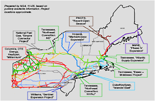
FIGURE D-4-1 Proposed Northeast pipeline projects. SOURCE: Northeast Gas Association. Available at http://www.northeastgas.org/pdf/pipe_enhance1105.pdf. Accessed February 2006. Reproduced with the permission of the Northeast Gas Association.
APPENDIX D-5
COAL TECHNOLOGIES
James R. Katzer1
Coal was used to produce 51 percent of the electricity generated in the United States in 2004. Domestic coal reserves are far greater than those of oil or natural gas, and costs for using coal to generate electricity are much lower than for oil and natural gas. Thus, coal promises to continue its position as the primary fuel for power generation for the foreseeable future. Pennsylvania, West Virginia, and other states have large resources of coal that could be delivered to New York relatively inexpensively.
Coal can contain high concentrations of ash and substantial amounts of sulfur, in addition to other toxic elements. It thus has the potential for high emissions, but appropriate control technology can reduce these emissions to a very low level.
Large coal-fired power plants are expensive to build and require substantial infrastructure for the delivery and storage of coal and the removal of ash and other captured pollutants. A much larger area is required for a coal plant than for a natural gas combined-cycle (NGCC) plant. Thus, coal plants require careful site selection and design. Even then, their impact on the environment and local communities can be greater than that of nuclear plants.
Pulverized coal combustion is the primary technology used to generate electricity from coal. Flue-gas-treatment technology to control emissions on new coal plants is very effective in reducing criteria emissions to very low levels. Plant generating efficiency can range from about 35 percent to as high as 43 percent for ultrasupercritical steam technology.
Fluidized-bed technology is another approach to coal combustion which, compared with pulverized coal combustion, offers much broader operating flexibility with respect to coal type. It also allows the combustion of a range of other materials mixed with the coal, such as the co-firing of biomass, wood wastes, and so on. Efficiency and emissions control are similar to that of pulverized coal.
Integrated gasification combined cycle (IGCC) involves gasification of coal to produce synthesis gas, cleaning the syngas, and then burning it in a combustion turbine. The power generation block for an IGCC plant is similar to that of an NGCC plant. The syngas-burning combustion turbine is connected to a generator; the steam raised from cooling the turbine exhaust powers a steam turbine. Typical generating efficiency is about 39 percent. The technology is commercial, but issues of operability and availability need further resolution. With IGCC, emissions including mercury and other toxics can be extremely low (unlike the case of pulverized coal with current technology), because the gases are all fully contained at high pressure. Coal ash from the IGCC process is fused and exits as a much less-leachable solid than fly ash. IGCC also allows for co-firing with biomass. Gasification provides for the most effective route to the capture of carbon dioxide for sequestration, and IGCC is projected to produce the lowest-cost power from any technology with carbon dioxide capture.
Whereas coal-fired power plants produce the lowest-cost power (without carbon dioxide capture), the requirements for large sites and extensive infrastructure limit the potential for the New York City area. In addition, air emissions and other environmental and community issues are likely to create considerable opposition to them in heavily populated areas. High capital costs and uncertainty of success in construction are likely to discourage investors. Nevertheless, the potential, particularly of the advanced IGCC technology, is so great that coal should be considered an option, at least for New York’s upstate regions. The remainder of Appendix D-5 explores emissions control, probably the most contentious issue for coal plants.
Emissions Control for Pulverized Coal (PC) Combustion Units
Typical flue-gas-cleaning configurations for coal-fired power plants are shown in Figure D-5-1. U.S. emissions data are typically given in terms of energy input—for example, pounds per million British thermal units (Btu)—and are thus independent of generating efficiency. This does not drive generating efficiency, as would an emissions limit based on output, such as pounds per megawatt (electric)-hour (MWe-h). Emissions below are presented in milligrams per cubic meter (mg/Nm3). The pulverized coal (PC) emissions are typically for supercritical PC units that are operating at about 39 percent (higher heating value [HHV]). Those for IGCC are for a unit that has 38 to 40 percent efficiency (HHV).
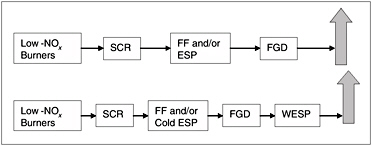
FIGURE D-5-1 Emissions control options for coal-fired generation. NOTE: NOx: oxides of nitrogen; SCR: selective catalytic reduction; FF: fabric filter; ESP: electrostatic precipitation; FGD: flue-gas desulfurization; WESP: wet ESP.
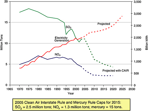
FIGURE D-5-2 Past and projected U.S. emissions from fossil power generation, 1965 to 2030.
Figure D-5-2 shows how emissions of SOx and NOx are likely to continue to decline for many years, despite growing electricity generation. Figure D-5-3 compares the emissions potential for various technologies. Table D-5-1 lists the cost of electricity with various levels of emissions control.
Particulate Control
Particulate control is typically accomplished with electrostatic precipitators (ESPs) or fabric filters. ESPs or fabric filters are installed on all U.S. PC units and routinely achieve >99 percent particulate removal. Greater particulate control is possible with enhanced performance units or with the addition of wet ESP (WESP) after flue-gas desulfurization (FGD) (Oskarsson et al., 1997), as illustrated in the second set of technologies in Figure D-5-1. The addition of wet ESP is beginning to become standard U.S. practice for new units to control condensable particulate matter (PM) and should achieve emissions levels less than 5 mg/Nm3 at 6 percent O2. Typical emissions for modern, efficient, U.S. PC units are 15 to 20 mg/Nm3. New units in Japan are achieving 5 mg/ Nm3 (PowerClean, 2004). Level of control is affected by coal type, sulfur content, and ash properties.
SOxControl
Partial flue-gas desulfurization is accomplished by dry injection of limestone into the ductwork just behind the air preheater for 50-70 percent removal, with recovery of the solids in the ESP. Wet flue-gas desulfurization (wet lime scrubbing) can achieve 95 percent SOx removal without additives and 99+ percent SOx removal with additives (Oskarrson et al., 1997; “Emissions Performance of PC Units,” personal communication from ALSTOM, Windsor, Connecticut, 2005). Wet flue-gas desulfurization has the greatest share of the market in the United States, is well proven, and is commercially established. Typical U.S. commercial performance is 150 to 170 mg/Nm3 at 6 percent O2,2 because this is what their permits require. Recently permitted units have much lower limits, and still lower emissions levels can
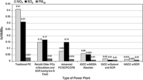
FIGURE D-5-3 Types of power plants.
be expected as permit levels are further reduced. The technology has not reached its limit of control. The best PC units in the United States burning high-sulfur bituminous coal are achieving demonstrated performance of less than 0.04 lb SO2/MMBtu or 40 mg/Nm3 (“Emissions Performance of PC Units,” personal communication from ALSTOM, Windsor, Connecticut, 2005); those in Japan operate below 75 mg/ Nm3. The wet sludge from the FGD unit must be disposed of safely.
NOxControl
Low-NOx combustion technologies, which are very low cost, are always used and give up to a 50 percent reduction
TABLE D-5-1 Electricity Cost from Coal with EmissionsControls
|
Level of Emissions Control |
Cost of Electricity (cents/kWe-h) |
|
PC generation without SOx or NOx controls, but with ESP for particulates |
4.08 |
|
Today’s PC unit with SOx and NOx controls |
4.75 |
|
2015 PC unit, tighter SOx, NOx, and mercury |
4.97 |
from noncontrolled combustion. The most effective, but also the most expensive, technology is selective catalytic reduction (SCR), which can achieve >90 percent NOx reduction over inlet concentration. Selective noncatalytic reduction falls between these two in effectiveness and cost. Today, SCR is the technology of choice to meet very low NOx levels. Typical U.S. commercial emissions control performance is 65 to 90 mg/Nm3. The best PC units in the United States are achieving demonstrated performance of 0.03 lb NOx/ MMBtu or 30 mg/Nm3 on sub-bituminous coal and 60 mg/ Nm3 on bituminous coal. The Parish plant, burning Powder River Basin coal, is achieving 0.03 lb/MMBtu, which is 30 mg/Nm3. The best PC units in Japan are achieving 30 to 50 mg/Nm3 at 6 percent O2.
Mercury Control
Mercury in the flue gas is in the elemental and oxidized forms, both in the vapor and as mercury that has reacted with the fly ash. This third form of emissions is removed with the fly ash, resulting in 10 to 30 percent removal for bituminous coals, but less than 10 percent for sub-bituminous coals and lignite. The oxidized form is effectively removed by wet FGD scrubbing, resulting in 40-60 percent removal for bituminous coals and less than 30-40 percent removal for sub-bituminous coals and lignite. For low-sulfur sub-bituminous coals and particularly lignite, most of the mercury is in the elemental form, which is not removed by wet FGD scrub-
bing. SCR for NOx control can convert up to 60 percent of the elemental mercury to the oxidized form, which is removed by FGD (EPA, 2005). Additional mercury removal can be achieved with activated carbon injection and an added fiber filter to collect the carbon. This technique can achieve 85-95 percent removal of the mercury. Commercial short-duration tests with powdered, activated carbon injection have shown removal rates around 90 percent for bituminous coals but lower for sub-bituminous coals (EPA, 2005). Research and development are currently evaluating improved technology that could reduce costs and improve effectiveness. The general consensus in the industry is that improved technology will change this picture significantly within the next few years.
Emissions Control for Integrated Gasification Combined-Cycle Technology
IGCC has inherent advantages for emissions control because the cleanup occurs in the syngas, which is contained at high pressure, and contaminants have high partial pressures. Thus, removal can be more effective and economical than cleaning up large volumes of low-pressure flue gas.
Particulate Control
The coal ash is primarily converted to a fused slag, which is about 50 percent less in volume and is less leachable than fly ash; as such, it can be more easily disposed of safely. Particulate emissions from existing IGCC units vary from 1 to 8 lb/MWe-h. Most of these emissions come from the cooling towers and not from the turbine exhaust and as such are probably characteristic of any generating unit with large cooling towers. This means that particulate emissions in the stack gas are below about 1 mg/Nm3.
SOxControl
Commercial processes such as MDEA and Selexol can remove more than 99 percent of the sulfur so that the syngas has a concentration of sulfur compounds that is less than 5 parts per million by volume (ppmv). The Rectisol process, which is more expensive, can reduce the SOx concentration to less than 0.1 ppmv (Korens, 2002). SO2 emissions of 0.15 lb/MWe-h, or 5.7 mg/Nm3 (2 ppm) have been demonstrated at the ELCOGAS plant in Puertollano, Spain (Thompson, 2005), and at the new IGCC plant in Japan. Recovered sulfur can be converted to elemental sulfur or sulfuric acid.
NOxControl
NOx emissions from IGCC are similar to those from a natural-gas-fired combined-cycle plant. Dilution of syngas with nitrogen and water is used to reduce flame temperature and to lower NOx formation to below 15 ppm. Further reduction to single-digit levels is achievable with SCR. NOx emissions of 4.2 mg/Nm3 (2 ppm) NOx (at 15 percent O2) have been demonstrated commercially in the new IGCC unit in Japan.
Mercury Control
Commercial technology for mercury removal in carbon beds is available. For natural gas processing 99.9 percent removal has been demonstrated, as has 95 percent removal from syngas (Parsons, 2002). Mercury and other toxics that are also co-captured in carbon beds produce a very small volume of material, which must be handled as a hazardous waste. Carbon capture will likely inhibit re-release into the environment.
Water Usage
PC and IGCC technologies both use significant quantities of water, and treatment and recycling are increasingly important issues. IGCC uses 20 to 50 percent less water than do PC plants. Wastewater treatment technology has been demonstrated for both technologies. Proven water treatment technology is available to handle the water effluents from each technology.
APPENDIX D-6
GENERATION TECHNOLOGIES—WIND AND BIOMASS
Dan Arvizu1
This paper summarizes an analysis performed by NREL under my direction and supervision to evaluate the potential of wind energy and biomass resources to generate electricity to meet the future energy needs in the area currently supplied by the Indian Point Nuclear Power Plant near New York City. This analysis discusses the potential for three sources of wind energy and several sources of biomass, and the underlying assumptions and issues related to the projections of potential.
Some important observations include the following:
-
The technical potentials (market size constrained only by the ability of technology to meet customer need and not by economics or other considerations) for both wind and biomass are very substantial, on the order of 9-10 GW in the Indian Point service area.
-
The achievable potentials for both are significantly less than the technical potential, on the order of 3 GW in 2014, but still substantial enough to replace the Indian Point capacity by that time.
-
Wind systems can be placed in the Hudson Valley right now, and, to a small extent, in the rural areas (northeast) of Long Island, within 10 miles of a transmission corridor.
-
Offshore wind could meet most of the Indian Point load by 2014. Canadian wind and hydro are reasonable options to explore in the meantime.
-
Biomass in the form of municipal solid waste could provide half of the Indian Point capacity in 2014.
-
Studies should continue to resolve wind-related issues such as transmission, dispatchability, siting and permitting, and biomass-related issues such as public perception, improved technology costs, and tipping fees.
Table D-6-1 summarizes quantitatively the potential impact of wind and biomass resources on the Indian Point service area, both in terms of technical potential and achievable potential.
Wind Contribution
Much relevant work has been done recently and is currently underway regarding wind power in New York. This analysis will outline broad issues and deployment options that could be considered as part of the electrical energy and capacity replacement, with reference to the recent work.
In addition to being renewable, wind power has characteristics that are different than conventional, dispatchable resources. First, the “fuel” source is controlled by nature, resulting in variable power output that is not controlled by the utility schedulers and dispatchers. This has two main implications to consider: (1) the capacity credit in the long term and the reliability value of wind to meet peak demand, and (2) the impact of wind variability on grid operations in the short term resulting from increased regulation, load following, and unit commitment burdens on other generators.
Second, the “fuel” cannot be transported. The wind turbines must be located in areas of good wind resource, which may or may not have access to existing transmission lines. Therefore, any comprehensive look at wind power potential must factor in questions such as:
-
Proximity of wind resources to the existing grid,
-
Available transmission capacity on existing lines (temporal profiles can be important),
-
Potential for upgrading capacity of existing lines and existing corridors, and
-
Costs and siting issues for any necessary new transmission connections.
The analysis below broadly discusses three wind-based options, including issues of resource, cost, reliability, and transmission (deliverability). The purpose is to broadly describe what is known, what the quantitative potentials may be, and what remaining issues could be examined to further define the potential.
Option 1: Land-Base, In-State Wind Development
Resources
-
There is adequate raw and developable wind resource in the state to generate the energy equivalent of Indian Point, over and above current state RPS needs.
-
In the future, increased hub heights, low wind speed turbine developments, and better wind resource information will likely expand the resource estimate.
-
Site-specific permitting issues may remain, and could be impacted by local and state policy.
Costs
-
Generally, land-based bus bar wind costs are in the 3-7¢/kWh range (not including the federal 10-year 1.8¢/kWh Production Tax Credit, which currently applies to projects online by 12/31/05).
-
Costs are expected to continue to decline incrementally due to increased efficiency, taller towers, and manufacturing volume. (However, it should be noted that near-term costs have increased slightly due to the euro exchange rate, cost of steel, and other temporary factors.)
TABLE D-6-1 Estimate of Potential Impact of Renewable Generation Technologies on Indian Point Service Area
|
|
Today |
2009 |
2014 |
|||
|
Wind and Biomass Potential |
Capacity (MW) |
Generation (GWh) |
Capacity (MW) |
Generation (GWh) |
Capacity (MW) |
Generation (GWh) |
|
Tehnical |
|
|
|
|
|
|
|
Wind onshore |
2,294 |
5,310 |
2,294 |
5,310 |
2,294 |
5,310 |
|
Wind offshore |
5,200 |
17,082 |
5,200 |
17,082 |
5,200 |
17,082 |
|
Biomass |
1,502 |
10,560 |
1,502 |
10,560 |
2,233 |
15,680 |
|
Subtotal |
8,996 |
32,952 |
8,996 |
32,952 |
9,727 |
38,072 |
|
Achievable |
|
|
|
|
|
|
|
Wind onshore |
0 |
0 |
229 |
531 |
459 |
1,062 |
|
Wind offshore |
0 |
0 |
300 |
986 |
1,800 |
5,913 |
|
Biomass |
234 |
1,640 |
386 |
2,705 |
1,137 |
7,968 |
|
Subtotal |
234 |
1,640 |
915 |
4,222 |
3,396 |
14,943 |
|
SOURCE: NYSERDA (2003). |
||||||
-
Further examination of the details of the GE/ NYSERDA wind integration and the Regional Greenhouse Gas Initiative work would likely yield specific site-based cost/supply curves.
-
Additional grid operating costs have been found to be in the 0.2-0.5 ¢/kWh range for a variety of U.S. utilities and up to 20 percent penetration by nameplate.
-
Operating costs were considered in the GE/NYSERDA study, but these additional costs were not reported separately from total costs. Little regulation impact and no impact on reserve requirements were found. Scheduling impacts were identified, and improvements in forecasting could bring costs down.
-
Specific operational costs for higher wind generation scenarios are unknown, but the study framework and methods exist.
-
For the GE 3,300-MW wind scenario, the increase in system costs was projected to range between $582 million and $762 million for renewable projects. It is expected to be offset by approximately $362 million in wholesale energy cost reductions as New York reduces its reliance upon fossil fuels.
Transmission
-
The GE study examined load-flow impacts of a 3,300-MW wind generation scenario for RPS compliance and found no significant upgrade needs.
-
Grid stability was found to be generally enhanced by the installation of new turbine technology incorporating power electronics and fault ride-through capability.
-
Much of the land-based resource is located upstate, on the wrong side of the bottlenecks near Indian Point.
-
Likely, significant upstate wind additions for Indian Point replacement would require some grid reinforcement. Specific needs are speculative, but the study methods and data are known.
-
Generally, transmission costs, including new lines, are an order of magnitude lower than generation costs.
-
Transmission permitting and construction times are in the 10-year time frame. Wind plants can come online in 1-3 years total. Grid operators in TX and CA are examining innovative solutions to this mismatch.
-
Due to resource variability, the potential exists for average line utilization factors to be low on lines serving primarily wind generation.
-
Temporal line loading profiles could be examined to determine if increased wind energy could flow on existing lines with limited curtailment during critical times.
Reliability
-
Effective load carrying capability studies in the GE/ NYSERDA study show low values, averaging 10 percent, therefore a land-based wind-only replacement of the peak load capability of Indian Point is not feasible.
-
Other opportunities could be examined to complement the energy-dominated value of wind with other generators, including:
-
Hydro: In-state resources of around 4.5 GW have an average utilization factor of around 50 percent, indicating a water-limited resource. If other flow regulations (environmental, recreation, etc.) allow, water could be retained for peak demand needs as a result of wind energy meeting off-peak and shoulder needs.
-
Simple cycle fast ramp generators: Simulations show an economic advantage for new, low-capital-cost gas generation run for very minimal peak hours in conjunction with wind as an optimum solution (saving expensive gas, but getting reliability benefit). These “super peakers” can also be located optimally on the transmission system.
-
Other electric storage systems could potentially help: pumped hydro, and compressed air being the most economical. Longer term, a transition to plug-in hybrid vehicles could
-
-
expand wind electricity markets and also provide grid storage support.
Option 2: Offshore Wind Development
Resources
-
Shallow water resources (up to 20 m depth) exceed 5 GW potential for class 5 and above for Long Island. Deeper water resources (20-40 m depth) off Long Island exceed 40 GW potential.
-
Permitting issues for federal waters (>3 miles) are in flux, but the Long Island Power Authority is currently negotiating with a developer for a 160-MW development within the state water boundaries.
-
Visual and other concerns seem to be much less off Long Island than those associated with the Cape Wind project in Massachusetts.
-
Technologies for deeper water are under development, including deep water floating and tethered concepts. Great amounts of resources exist in these waters.
Costs
-
Off-shore capital cost estimates begin at $1,500/kW (roughly 50 percent more than on-shore) and go up. Euro-pean experience is relevant up to about 30 m depth. Higher, steadier wind speeds increase energy production, but O&M costs are generally higher. Current levelized cost is around 6¢/kWh at best.
-
Costs are expected to decline significantly, perhaps to less than 4¢ in shallow water, in the next decade.
-
Grid-operating cost additions would be expected to be similar to on-shore, with the possible caution that limited data from Horns Rev in Europe shows some higher ramp rates than on-shore.
Transmission
-
Off-shore is generally envisioned as being deployed near load centers. Some on-shore reinforcement may be needed, and an off-shore cable is needed. However, costs should be lower and siting difficulties should be minimal compared to on-shore transmission expansion.
-
The Long-Island off shore resource is on the load side of the transmission bottlenecks around Indian Point, further alleviating transmission concerns.
Reliability
-
The GE study found an effective load carrying capability (capacity factor) of 30 percent for Long Island off-shore resources. This is promising compared to on-shore.
-
Further study of great lakes resources would be necessary to quantify possible diversity benefits of multiple offshore locations.
-
All the generator synergistic and storage options discussed in on-shore could apply here, but needs might be a factor of three less per MW of wind.
Option 3: Imported Canadian Wind, Firmed with Canadian Hydro
Resources
-
Canadian wind and hydro resources appear vast; further examination is needed.
-
Hydro Quebec imports some energy into New York already, and is willing to look at more, including wind/hydro blends.
-
There is some reluctance to promote additional large Canadian hydro for U.S. demand due to environmental and native population concerns.
Costs
-
Wind power costs should be similar to the U.S. land-based resources.
-
Operating cost additions from hydro are not well characterized, but should be minimal.
-
Bonneville Power in the United States has offered a shaping and firming product for wind that delivers a schedulable, flat block of equivalent wind power for an additional 0.6¢/kWh. Recent discussions indicate this price is well over actual cost and the price may drop as the utility gets more experience with the service.
-
Canadian hydro seems to be much less constrained by other river criteria than in the United States, so costs of variability mitigation would be expected to be much lower.
Transmission
-
Studies of the capability of existing lines for importing additional power from Canada should be available, but were not researched.
-
At 2-GW levels, DC options become advantageous for new long lines. This could be considered for direct connection to and near-equivalent replacement of Indian Point. Hydro firming could essentially base-load the wind and levelize the transmission line loading at near full capacity.
Reliability
-
Hydro firming will essentially turn the wind into a base-load resource with equivalent reliability to Indian Point.
-
Options for shaping the energy to fit the full peaking and load following needs could also be examined, with some incremental impact on transmission due to lower average loading factors and/or higher line capacity needs.
Quantitative Estimates for Wind
Estimates of wind resources in New York electric zones G, H, I, J, and K are presented in Table D-6-2. These zones are south of the major transmission bottlenecks from upstate New York generation to the New York City load. Therefore, adding wind generation in these zones is not likely to require significant upgrade or additional transmission line construction. This analysis used a high-resolution
TABLE D-6-2 Quantitative Estimates of Wind Potential in Indian Point Zones
|
Zone |
Complete Wind Resource, After Environmental Exclusions; Power Class 3, 4, 5, and above |
Resource Within 10 Miles of Existing Transmission; Power Class 3, 4, 5, and above |
Postulated Possible Development (out of 10 GW total) in GE NYSERDA Renewable Portfolio Standard Study |
|
Zone G |
528, 129, 90 MW |
436, 110, 84 MW |
154 MW |
|
Zone H |
0, 0, 0 |
0, 0, 0 |
0 |
|
Zone I |
0, 0, 0 |
0, 0, 0 |
0 |
|
Zone J |
0, 0, 0 |
0, 0, 0 |
0 |
|
Zone K |
2,116, 431, 73 MW (onshore)a |
1,482, 177, 5 MW (onshore) |
600 MW |
|
NOTE: The wind resource potential is essentially constant with time, so the numbers can be used over the complete 2007-2015 study time frame. Between-turbine spacing to prevent excessive induced downwind turbulence is normally computed as a multiple of rotor diameter. In this assessment we have assumed a turbine density of 5 MW per square kilometer, independent of turbine size. Energy output per unit of nameplate capacity is expected to increase slightly over the time period due to incremental improvement in machine efficiency and higher average wind speeds resulting from increasing tower height. Because of increased energy delivery, there may be a corresponding incremental increase in reliability (capacity credit) values. aOver 5,200 MW of offshore class 5 and better wind is located in water less than 20 m deep. bOffshore within state 3 mile limit. |
|||
wind map produced for NYSERDA by AWS Truewind in 2000. Higher-resolution data should now be available, and the analysis should be repeated.
As noted above, GE Energy and AWS Truewind Solutions have recently completed a look at integrating 3,300 MW of additional wind spread around the New York grid, finding no need for significant transmission upgrades or reliability issues. In selecting locations for the 3,300 MW, GE identified 10 GW of likely wind locations. Much of that wind generation was postulated in upstate areas. For comparison purposes, the last column in Table D-6-2 shows how much of the 10 GW scenario is in each of the generation zones in question.
The numbers presented in Table D-6-2 assume 5 MW per square kilometer of windy land. Values are net after subtracting environmental exclusions defined as all national Park Service, Fish and Wildlife, other specially designated federal lands such as wilderness areas, monuments, etc., all highly protected as determined by land stewardship data from the Gap Analysis Program (GAP) of the U.S. Geological Survey, and half of the second highest GAP land stewardship category, remaining U.S. Forest Service, and Department of Defense land. No other land use exclusions were subtracted.
As shown, there is some potential for wind in the immediate vicinity of Indian Point. Most of the wind potential in Zone G is close to existing transmission corridors. However, Zones H, I, and J are some of the least windy areas of the state. Long Island shows significant onshore and offshore wind resource potential. Note again that offshore wind power peak times show a much better match to peak electric load demand as measured by Effective Load Carrying Capability (reliability-based capacity credit) than on-shore resources. The operational, reliability, and transmission impacts of wind as a potential part of Indian Point replacement is best examined with detailed grid simulation. This will provide much better data on least cost solutions that may incorporate significant amounts of wind outside the zones tabulated in Table D-6-2.
Wind-Related Policy Options
-
On a $/MWh basis, wind is likely to be a low-cost, in-state option in 2007-2015, so broad state economic subsidy policy drivers may not be necessary.
-
It is likely that near- to mid-term worldwide markets for wind hardware will be supply limited. Manufacturing incentives may help build up supply capability, and help state economic development as well.
-
Wind is primarily an energy, not capacity source, so that system reliability issues are important. The GE tools called MARS (Multi-Area Reliability Simulator) and MAPS (Multi-Area Production Simulator) are a good framework for the grid issues to be examined. GE could examine scenarios that include reliability synergies of possible benefit to wind, including:
-
In-state hydro dispatch modifications
-
Canadian hydro contract modifications to provide additional ancillary services (indications are they have dispatch flexibility)
-
Options for additional Canadian hydro (it appears current Day Ahead and Real Time Hydro Quebec imports are bounded at about 1,500 MW, so additional transmission may be needed)
-
-
Examination of competitive market structures that would motivate other resources to provide additional ancillary service levels
-
Examination of transportation market modifications (plug hybrids and hydrogen) that would decrease the need for grid ancillary services imposed by wind
-
Grid-level issues like transmission and operational issues for increased wind deployment should continue to be examined, through public funded mechanisms like NYSERDA or through allowing NYISO or others to recover appropriate costs from ratepayers.
-
Siting and permitting issues for both land-based and off-shore wind plants should be addressed, including proactive examination of potential wildlife issues.
-
Transmission costs are not large adders to generation costs. It is almost always cheaper to build transmission to a better wind resource than to use lower-class, closer wind. Transmission planning, siting, cost recovery, and construction issues need to be examined to reduce uncertainty and shorten the in-service timelines, if new transmission is necessary to serve wind.
Biomass Contribution
Primary Source
There have been extensive studies of the renewable biomass potential in New York. Information summarized in this analysis has been gleaned from the NYSERDA report Energy Efficiency and Renewable Energy Resource Development Potential in New York State—Final Report, dated Au-gust 2003. (Prepared by Optimal Energy Inc., ACEEE, Vermont Energy Investment Corporation, and Christine T. Donovan Associates.)
Geographical Basis
The zones of interest in the NYSERDA report are G, H, I, J, and K. Since biomass is generally assigned on a county basis, the relevant counties are (again working northwest to southeast): Delaware, Ulster, Green, Columbia, Sullivan, Dutchess, Orange, Putnam, Rockland, Westchester (location of Indian Point), Richmond, Nassau, and Suffolk. The report also has time horizons of 2007, 2012, and 2022.
Background on Biomass Availability
The regions other than Delaware, Sullivan, and Ulster are increasingly heavily populated as one goes from NW to SE. Thus six of the existing 10 waste-to-energy facilities are in this region. These six already generate 68 percent of the total 2.15 TWh generated in 2000. The region’s net capacity is 156 MW.
Urban residues are a huge resource, but are not viewed as “clean” from the NY-RPS definition. Public acceptance is low and to comply with federal, state, and local regulations, the cost of the facilities has reached over 8,000 $/kW.2 Thus even with a tipping fee, there is presently a lower-cost alternative in burial of the wastes out of state.
The report assumes continuing use of mass burn technology. For the regions defined above, the capacity would be unchanged until 2012 when the report proposes 76 MW additional located in NYC. By 2022 a further 166 MW would be added, also in NYC.
Cleaner biomass resources include: mill residues (from primary and secondary wood processing); silviculture residues; site and land conversion residues; wood harvest; yard trimmings; construction and demolition (C&D) wood; pal-lets; agricultural residues; bio-energy crops; animal and avian “manure,” and wastewater methane.
Supply curve: Ideally the availability of these resources could be combined with the potential technologies to derive a supply curve—GWh vs cost. The current data is not adequate to do this at the regional scale. Statewide the sum of these resources amounts to 0.24 quad in 2003, and 0.4 quad in 2022, with the increase primarily due to a large energy crop contribution. In the regions identified for the Hudson Valley to Long Island, the resource base is primarily urban residues (ranging from MSW to C&D wood) in the timeframe to 2012. After 2012 additional energy crop biomass could be developed. For this region the assumption is that the 2012 availability would about 0.015 quad. Upstate New York has a far higher potential due to forest and agricultural potentials.
Table D-1-3 assumes two biomass prices—biomass (e.g wood chips from forestry operations) at $2.50/106 Btu, and MSW at –$2.50/106 Btu. The negative cost reflects a tipping fee. A reasonable blended price for the urban residue generation in the zones considered would be $1.00/106 Btu (2002). More detailed study would be needed to arrive at a more precise estimate of the proportions of material with a significant tipping fee, and those for which transportation would be a larger factor.
Technical potential: Applying these resources to the load zones G, J, and K, the 2003 technical potential would be 203 MW generating 1.423 TWh (capacity factor is 7,000 h/y, heat rate 10,500 Btu/kWh, i.e., 32 percent efficient). The technical potential in 2022 would be 295 MW, with the main part of the growth being in the Hudson Valley (zone G).
Technologies
There are three technologies in the NYSERDA report: CHP, co-fire, and gasification. Assumptions in the report are
for CHP to grow statewide, mainly in the pulp and paper sector. However, in the regions of interest, there would be a zero contribution of CHP.
Co-fire would be possible in the Hudson Valley. However, this is not an incremental generation of net power as the biomass displaces coal in an existing facility. Approximately 100 MW of the potential 203 MW would be in co-firing in the report.
Gasification in the study would be applied to low-cost construction and demolition debris more or less at the point of generation in NYC (zone J) with approximately 100 MW capacity.
Conclusion from the 2003 Report
The near-term potential in the region is about 200 MW with an 80 percent annual capacity factor. With attention to energy crops in the Hudson Valley this could increase to 300 MW. A further increment could come from the urban residue stream but would require a change in technology to overcome public resistance and very high investment cost barriers.
Economics: Assuming that gasification was to be used for all biopower applications (i.e., no CHP or co-firing contribution), the economic parameters assumed include an investment level (2002) of $1,700/kW, and a fuel cost of about $1/GJ. This fuel cost is a blended price from very low cost C&D material to some forest residues at $2.50/GJ. The proposed technology is based on an IC engine technology with a medium-heating-value gasifier system. The scale would be in the range of 20-40 MW with a heat rate of 35 percent (9,000 Btu kWh–1). The fleet of gasification IC engine units would be between 5 and 12 depending on size. Modularity is assumed as well as a series production of units to achieve the investment cost proposed.
Cost per kWh: Using the same financial assumptions as in Appendix D-1 above, the busbar cost before distribution would be $0.045/kWh.
An Alternative View
Table D-6-3 contains both technical potential data and an estimate of achievable potential that exceeds the values proposed on the basis of the Energy Efficiency and Renewable Energy Resource Development Potential in New York State—Final Report, dated August 2003. Similar cost and performance of the biomass-to-electric technologies are assumed in the report and Table D-6-3, such that the technical potential is the same. The differences in achievable potential result from valid differences in optimism about economics, technology, and non-monetary barriers.
The New York State report was constrained by an economic assumption framework for a period up to about 2001. This is essentially a business-as-usual framework that did not assume the loss of the nuclear capacity, nor the recent rapid changes in fossil energy prices (coal, oil, and gas), nor the more aggressive renewable energy framework of state RPS and increased federal and state incentives. Thus, for MSW/CDW shown in Table D-6-3, the difference between 398 MW in 2022 in the report, and the achievable potential
TABLE D-6-3 Biomass Potential Applicable to Indian Point
|
|
Today |
2009 |
20014 |
||
|
Potential |
Capacity (MW) |
Capacity (MW) |
Generation (TWh) |
Capacity (MW) |
Generation (TWh) |
|
Achievable |
|
|
|
|
|
|
MSW/CDW |
233.8 |
365 |
2.56 |
1,096 |
7.68 |
|
Biogas (Sewage) |
|
20 |
0.14 |
41 |
0.32 |
|
Total biomass |
|
386 |
2.72 |
1,137 |
8.00 |
|
Technical |
|
|
|
|
|
|
MSW/CDW |
|
1,461 |
10.24 |
2,192 |
15.36 |
|
Biogas |
|
41 |
0.32 |
41 |
0.32 |
|
Total biomass |
|
1,502 |
10.56 |
2,233 |
15.68 |
|
NOTE: Counties in region: Bronx, Kings, New York, Queens, Richmond, Columbia, Delaware, Dutchess, Greene, Nassau, Orange, Putnam, Rockland, Suffolk, Sullivan, Ulster, Westchester. Population data—New York State Data Center, http://www.nylovebiz.com/nysdc/data_economic.asp (Aug 10, 2005). MSW per capita generation—national average from Biocycle, Apr 2004, v45, n4, p22 (1.31 ton/per capita/annum); this number includes C&D wood. Biogas = 1 ft/per capita/day@640 Btu/ft3 Roberts and Hagen, UC Davis, 1978. Existing Capacity, Renewable Electric Plant Information System, NREL, 2002 data. Assumption for solid feeds: 80% capacity factor, 20% efficiency in 2009, 30% efficiency in 2014. Assumption for biogas: 35% efficiency, 80% capacity factor. Did not factor in population growth for this version. Existing generation is for 2004, estimated from EIA Form 906. |
|||||
of 1,096 MW for 2014, represents the difference between a very conservative forecast and one in which many of the nonmonetary barriers, and some of the cost barriers, are reduced.
The disparity can only be resolved by a more substantial analysis in which there is a regionwide supply curve for biomass electricity generation at specific locations based on GIS supply and demand analysis.
Supporting Discussion for Biomass Potential Table
Technical Potential
The amount of capacity or power which is possible by using a technology or practice in all applications in which it could technically be adopted, without consideration of its costs.
Assumptions
Counties in region—The counties are Bronx, Kings, New York, Queens, Richmond, Columbia, Delaware, Dutchess, Greene, Nassau, Orange, Putnam, Rockland, Suffolk, Sullivan, Ulster, Westchester
-
Population Data: 2004 estimate from the New York State Data Center (http://www.nylovebiz.com/nysdc/data_economic.asp, August 10, 2005). Population growth was not factored into the 2009 and 2014 estimates, but can be in future updates.
-
1.31 tons MSW per capita per year. This was the national average generation from Biocycle, Apr 2004, v45, n4, p22 (individual states not given). The number may include construction and demolition wood. Since then the actual Biocycle survey (“The State of Garbage in America,” Biocycle, January 2004) was obtained. The New York estimate is 1.29 tons/per capita/year. Since the value is close the original estimate was not corrected.
-
The existing capacity estimate was taken from the Renewable Electric Plant Information System (REPIS), NREL, 2002 data. The data are on a state and regional basis. Existing biogas generation (primarily landfill gas) was not included.
-
Existing generation was taken from the EIA Form 906/ 920 using 2004 data (http://www.eia.doe.gov/cneaf/electricity/page/eia906_920.html, August 10, 2005). Form 906 gives capacity and generation information for all power plants in the United States. Form 906 was not used for capacity since not all data entries include a reported capacity.
-
Assumed basis is higher heating value.
-
Biomass potential was based on Oak Ridge National Laboratory, Biomass Feedstock Availability in the United States, State Level Data, 1999.
-
Sewage biogas was estimated using 1 ft3/per capita/ per day with a heat content of 640 Btu/day based on an old reference: E.B. Roberts and R.M. Hagen, Guidelines for the Estimation of Total Energy Requirements of Municipal Wastewater Treatment Alternatives,” a report to the Califor-nia State Water Control Board, University of California at Davis, 1977.
-
MSW heating value (5,000) Btu/lb (dry) was taken from W.R. Niessen, C.H. Marks, and R.E. Sommerlad, 1996, Evaluation of Gasification and Novel Thermal Processes for the Treatment of Municipal Solid Waste, 196 pp., NREL Report No. TP-430-21612. Values used for wood and agriculture residues/energy crops were 8,000 and 7,500 Btu/ lb dry, respectively.
-
Efficiency and capacity assumptions
-
Biogas—35 percent efficiency (IC engine), 80 percent capacity factor
-
Solid feeds
-
20 percent efficiency (mass burn or stoker grate), 80 percent capacity factor from R.L. Bain, W.P. Amos, M. Downing, and R.L. Perlack, 2003, Biopower Technical Assessment: State of the Industry and the Technology, NREL Report No. TP-510-33123, Jan., Golden, CO.
-
30 percent efficiency (gasification), 80 percent capacity factor from W.R. Niessen, C.H. Marks, and R.E. Sommerlad, 1996, Evaluation of Gasification and Novel Thermal Processes for the Treatment of Municipal Solid Waste, 196 pp., NREL Report No. TP-430-21612.
-
-
Calculation Procedure
-
Biomass
-
Generation estimated by multiplying resource by heating value, converting to kW thermal, and multiplying by assumed efficiency to obtain kWh electric
-
The capacity factor was used to estimate capacity: MWh divided by hours per year divided by capacity factor.
-
-
MSW/CDW and Biogas
-
Generation estimated by multiplying population estimate (both regional and state) by per capita generation, multiplying by heating value, converting to kWh thermal, and multiplying by assumed efficiency to obtain kWh electric.
-
The capacity factor was used to estimate capacity: MWh divided by hours per year divided by capacity factor.
-
Market Potential
-
Technical Potential
-
Assumes 100 percent utilization of estimated feed-stock.
-
In 2009, the assumption is that the process will be mass burn or stoker grate for solid feeds.
-
In 2014, the assumption is that the process will be gasification for solid feeds.
-
IC engines at constant efficiency assumed for biogas.
-
Although co-firing is by far the least expensive option for electricity generation, it does not increase capacity, i.e., considered fuel substitution and was not included.
-
-
Achievable Potential
-
For Biomass and MSW/CDW
-
An RPS and a Section 45 tax credit are assumed as market intervention factors.
-
A Section 45 type credit (value not estimated) is extended to CHP systems heat production to encourage maximum process efficiency.
-
A 25 percent penetration is assumed in 2009.
-
With the use of higher efficiency, lower emissions, and lower-cost gasification technologies the penetration rate is increased to 50 percent in 2014.
-
For energy crops a low penetration is assumed, 5 percent in 2009 and 10 percent in 2014. The value is greater that zero to recognize the progress made in dedicated crops (willow) by projects such as the Salix project.
-
-
Since biogas (sewage) is already being generated, and because the generation of electricity should give lower emissions than flaring, a high penetration should occur. Fifty percent is assumed in 2009, and 100 percent in 2014.
APPENDIX D-7
DISTRIBUTED PHOTOVOLTAICS TO OFFSET DEMAND FOR ELECTRICITY
Dan Arvizu1
This appendix summarizes an analysis performed by NREL under my direction and supervision to evaluate the potential of distributed photovoltaics (PV) to offset the future electricity generation and capacity needs in the area currently supplied by the Indian Point Nuclear Power Plant near New York City. This analysis provides an overview of PV markets, an analysis of the potential for PV to help replace the electricity capacity and generation from the Indian Point nuclear power station in New York State, a summary of New York’s current policies related to PV technology, and an accelerated PV deployment scenario for New York through 2020.
Some important observations include:
-
The technical potential for rooftop PV in New York is very large—on the order of 35-40 GW statewide and 18-20 GW in the Hudson Valley, NYC, and Long Island control areas. Reaching this potential will require time to scale up the market infrastructure and production capacity for PV.
-
Given that PV is a distributed generation technology it competes against retail, not wholesale, electricity rates.
-
Given that PV is a distributed generation technology and that its production profile is highly coincident with peak demand it can contribute significantly to grid stability, reliability, and security. Thus, from a planning perspective PV should be valued at a rate higher than the average retail rate.
-
The cost of PV-generated electricity is expected to decline considerably over the next decade, falling from a current cost of 20-40 cents/kWh to a projected cost of 10-20 cents/kWh by 2015.
-
Given that Indian Point is a ~2 GW base load plant, operating roughly 95 percent of the time, it would be very difficult for PV alone to replace all of the generation from Indian Point during the next 5-10 years.
-
By pursuing a strategy that would combine PV with other technologies, such as efficiency, wind, hydro, and storage, PV should be able to replace 15-20 percent of the generation of Indian Point and 80-90 percent of the capacity of Indian Point during peak periods by 2020.
Under an aggressive but plausible accelerated PV deployment scenario, roughly 50 MW of PV systems could be installed in New York by 2009 (generating roughly 80 GWh of electricity), and 470 MW of PV systems could be installed in New York by 2014 (generating 700 GWh of electricity) (see Table D-7-1). This level of PV installations in 2014 could offset about 30 percent of Indian Point’s capacity during peak periods and about 4 percent of Indian Point’s annual electricity output. In addition, under the accelerated scenario about 1 GW of PV systems could be installed in New York by 2016, generating 1,500 GWh of electricity (offsetting about 40-50 percent of Indian Point’s capacity during peak periods and 9 percent of Indian Point’s annual electricity output). Realizing this accelerated scenario would require making a clear long-term commitment, in terms of both policies and resources, to expanding New York’s existing PV programs. Perhaps more importantly such an initiative would establish a self-sustaining PV market in New York, resulting in an additional 1 GW of PV being installed in New York by 2020, generating 3,000 GWh of electricity (offsetting about 80-90 percent of Indian Point’s capacity during peak periods and 18 percent of Indian Point’s annual electricity output) without any public subsidies between 2016 and 2020.
Key PV Markets
During the past decade the global PV market has been experiencing explosive growth. For example, during the past 5 years (1999-2004), the average annual growth rate of the global PV industry has been 42 percent. As shown in Figure D-7-1, the fastest growing PV market segments during this period were the grid-connected residential and grid-connected commercial segments. Such rapid growth has created tremendous excitement about PV technology around the world on the part of governments (EC, 2004), industry (SEIA, 2004; NEDO, 2004; EPIA, 2004), and the investment community (CLSA, 2004). As shown in Figure D-7-1, during 2004 the global PV industry passed the 1 GW mark in annual installations. At this point in time the global PV industry is truly beginning to move into large-scale production.
The rapid growth in the global PV market during the past decade, shown in Figure D-7-1, was driven largely by government subsidy programs, in particular in Japan, Germany, and a few states within the United States (including Califor-nia and New York). Over the coming decades, as costs con-
TABLE D-7-1 Estimated Distributed Photovoltaics in the Indian Point Service Area in the Accelerated Deployment Scenario
|
|
2005 |
2009 |
2014 |
2016 |
2020 |
|
Installed PV capacity (MW) |
2 |
56 |
470 |
1,000 |
2,000 |
|
Generation offset by PV(GWh) |
3 |
84 |
700 |
1,500 |
3,000 |
|
SOURCE: Derived from NYSERDA (2003). |
|||||
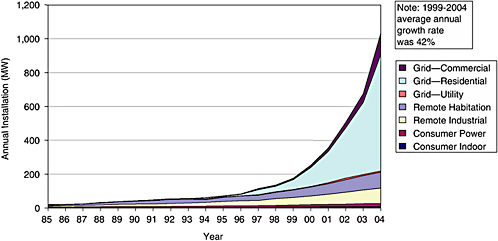
FIGURE D-7-1 Global PV market evolution by market segment, 1985 to 2004. SOURCE: Strategies Unlimited (2005).
tinue to decline and subsidies are phased out, industry analysts expect that the distributed grid-connected residential and grid-connected commercial markets will continue to expand rapidly and will become self-sustaining. Thus the grid-connected residential and commercial markets have emerged as key markets for developing and expanding the use of PV technology and are the logical place for New York State to focus its market development efforts over the next decade.
Technical Potential and Value of PV in New York State
The technical potential for grid-connected residential and commercial PV in New York State is very large—estimates of the rooftop technical potential in 2025 are on the order of 35-40 GW (NYSERDA, 2003; Navigant, 2004). If one considers only the Hudson Valley, NYC, and Long Island control areas, then the rooftop technical potential is on the order of 18-20 GW (NYSERDA 2003; Navigant 2004). This technical potential is enough to generate 27,000 GWh of electricity per year compared to the 16,700 GWh currently produced at Indian Point Units 1 and 2.
Expanding the market toward this technical potential, however, will require time to develop both the market infrastructure and production capacity for PV. As noted above, global PV production exceeded 1 GW in 2004. Given that Indian Point’s capacity is ~2 GW with a capacity factor of ~95 percent, and that PV in New York State has a capacity factor of ~17 percent, replacing the equivalent of Indian Point’s generation with PV alone would require an installed PV capacity of >10 GW in New York State. Thus it would be unrealistic to expect New York State to be able to fully replace the generation from Indian Point with PV alone during the next 5 to 10 years.
In thinking about the potential contribution PV could make towards replacing Indian Point, it is important to emphasis the technology’s best attributes, i.e., PV can provide high-value peak-time power in a distributed fashion and with zero environmental emissions. The ability to install PV in a distributed fashion combined with its production profile enable PV to contribute significantly to grid stability, reliability, and security (Perez et al., 2004b). Thus it would make sense to pursue a strategy that combines PV with energy conservation, other generation technologies (such as hydro and wind), and storage (e.g., a combination of pumped storage, compressed air energy storage, a variety of end-use storage technologies, etc.). Such a strategy would be designed to draw on the strengths of each of its components. For example, using hydro as a buffer for PV might be an attractive option. While major hydro facilities within New York State, such as Niagara Falls and Robert Moses (7 GW total), have limited buffers, it might be possible to use PV in combination with imported Canadian hydro. This strategy would utilize PV generation combined with a limited amount of local energy storage to displace expensive on-peak demand, i.e., when transmission is likely to be constrained and the market
TABLE D-7-2 Current and Projected Distributed PV Cost (2005 dollars)
clearing price is high, and to import Canadian hydro to meet off-peak demand, i.e., when transmission is available and the market clearing price is low.
With such a strategy PV might be able to realistically replace 15-20 percent of the generation of Indian Point and 80-90 percent of the capacity of Indian Point during peak periods by 2020 (the strategy as a whole would replace a much larger fraction of the generation from Indian Point). This strategy could be implemented starting in relatively small increments, installing 10s of MW during the first couple of years and increasing installations to about 200 MW per year by 2015, resulting in a total installed PV capacity of ~2 GW by 2020 (as illustrated in the accelerated PV deployment scenario discussed below). Such a goal could probably be achieved through a declining subsidy program that would enable the PV industry and market infrastructure to grow in New York State and enable regulators and policymakers to learn about how PV interacts with the grid in a controlled fashion.
Overview of PV Current and Projected Cost Through 2015
An overview of the current and projected cost through 2015 for PV technology is shown in Table D-7-2. As discussed above the two key markets for PV are assumed to be distributed residential systems and distributed commercial systems; thus the high/low ranges are based on current and projected costs in these two market segments. As shown in the table, the current levelized cost of energy is roughly 20-40 cents/kWh, and the projected levelized cost of energy in 2015 is roughly 10-20 cents/kWh.
It is important to note that the costs shown in Table D-7-2 are to the end user, i.e., they should be compared to retail rather than wholesale electricity rates. In addition, since the production from PV is highly coincident with peak demand in New York,2 a strong argument can be made for valuing PV in a planning context at a rate higher than the average retail rate in New York. For example, Perez et al. (2004a) used the average NYISO day ahead hourly wholesale price of electricity data in the NYC metro area and Long Island regions during 2002 to estimate the solar-weighted wholesale price, i.e., weighted by PV output. Using this detailed data they concluded that combining PV with a limited amount of load management (to enable PV to claim a capacity value close to 100 percent) would have increased the value (i.e., the systemwide cost savings) of residential PV during 2002 from 15 cents/kWh (the average retail rate) to 21.3 cents/kWh in NYC and from 12 cents/kWh (the average retail rate) to 20.3 cents/kWh on Long Island. As shown in Table D-7-2, if PV system owners could capture this value through interconnection rules, rate structures, etc., then PV technology could become a rapidly expanding and self-sustaining industry in New York State during the next decade.
Current Policies for PV in New York. New York has a fairly aggressive set of policies aimed at encouraging the adoption of PV technology. A detailed list of existing policies is provided in Table D-7-3. As shown in the table, New York has put in place a combination of tax exemptions and credits, loan subsidies, rebates (administered by LIPA and NYSERDA), and standard interconnection and net metering rules. Only New Jersey has created a more comprehensive set of incentives for residents and businesses to install PV in the Northeast.
As shown in Table D-7-3, New York has an existing rebate or “buy-down” program. The main program, administered by NYSERDA, is called New York Energy $mart and includes customers with all the major IOUs. New York Energy $mart provides customers who purchase and install PV systems with a $4/W rebate. This incentive in combination with state tax credits and exemptions has resulted in the installation of over 1.5 MW as of summer 2005. The program currently has $12 million allocated to its PV incentive program, of which about $6.5 million has been reserved as in-staller/customer incentives. The remaining funding should take the program through 2006.
LIPA, the public utility serving Long Island, also has an existing PV incentive program called the Solar Pioneer Program. LIPA launched the Solar Pioneer Program in 1999 and offered customers a substantial rebate. The rebate’s budget is tied into LIPA’s 5-year Clean Energy Initiative with a funding level totaling $37 million annually (covering multiple technologies). The Clean Energy Initiative is expected to receive funding through 2008. To date, 511 rebates have been disbursed for PV systems totaling more than 2.63 MW installed on Long Island. LIPA’s rebate is currently set at $4/W.
While the existing rebate programs are functioning well and expect to be fully subscribed this year, what is missing in New York is a clear long-term commitment of resources at the scale required to grow the PV industry in New York rapidly. Given New York’s relatively high electricity prices—the average residential electricity price in New York was 14.3 cents/kWh in 2003 (EIA, 2005)—and reasonably good solar resources, with a long-term commitment of sufficient resources New York should be able to accelerate the growth of PV substantially over the next decade.
An Accelerated PV Deployment Scenario for New York. The fact that the existing buy-down programs are well subscribed indicates that they are buying down the price of PV systems into a range that makes them economically attractive to consumers. Given that current installed system prices are about $8/W in New York, with a $4/W buy-down, the final cost to the consumer is about $4/W. If financed over the life of the system (30 years) at a 6 percent interest rate (~4 percent real interest rate after tax benefits) the levelized cost of energy from such a PV system would be about 13.5 cents/kWh. With an average residential electricity price above 14 cents/kWh in New York, combined with attractive net metering rules, it is not surprising that this investment would look reasonable to many consumers.
While such an investment might look attractive to consumers, it is of little value if consumers cannot find reputable installers. Here is where having a clear long-term policy commitment plays a critical role. Setting up a new business (getting certified, training staff, etc.) requires a substantial investment of resources. Entrepreneurs need to believe they will be able to recoup this investment over time. Policy uncertainty, in this context, creates a substantial barrier to building a viable local PV distribution, installation, and maintenance industry.
This accelerated scenario is modeled on the successful Japanese program that provided a declining subsidy to residential PV systems over the past decade, expanding residential PV installations in Japan from roughly 2 MW in 1994 to 800 MW in 2004 (Ikki, 2005). The history of the Japanese residential PV subsidy program during the past decade has provided proof that making such a long-term commitment to building the market infrastructure for PV can result in a self-sustaining industry. The average price of residential PV systems installed in Japan in 2004 was $6.2/W, i.e., about 25
TABLE D-7-3 Current PV-Related Policies in New York State
|
Incentivea |
Description |
|
Sales tax exemption (R) |
100% sales tax exemption |
|
Property tax exemption (C, I, R, A) |
15-year tax exemption for all solar improvements |
|
Personal tax credit (R) |
25% tax credit for PV (<10 kW) and SHW, capped at $5,000 |
|
State loan program (C, I, R, A, G) |
$20,000-$1 million loan for 10 years at 4-6.5% below the lender rate for PV and SHW |
|
State rebate program (C, I, R, A, G) |
$4-$4.50/W (<50 kW) up to 60% of total installed costs; IOU customers only |
|
Municipal utility rebate program (C, R, G) |
$4-$5/W (<10kW); LIPA customers only |
|
Interconnection standards (C, I, R, A) |
Standard agreement for PV requires additional insurance and an external disconnect; up to 2 MW max. |
|
Net metering standards (R, A) |
All utilities must credit customer monthly at the retail rate for PV systems under 10 kW |
|
aC = commercial; R = residential; I = industrial; A = agricultural; G = government. Incentive data available at <DSIRE.org 08/2005>. |
|
percent lower than in New York. This cost differential is a reflection of the difference between a well-functioning and emerging market for PV systems. PV modules and inverters are commodities whose prices are largely driven by international markets; however, labor and balance of system costs (which typically account for 30-40 percent of total system cost) are driven by local policies and market development.
Figure D-7-2 shows an accelerated market development path for New York. This scenario is not a model result, but an estimate of what New York could achieve under the fol-lowing assumptions:
-
The cost projection is in line with what the DOE Solar Energy Technology Program and the U.S. PV industry believe will be achieved over the next 10-15 years in the United States (DOE, 2004; SEIA, 2004)—in other words, it is an aggressive but plausible projection.
-
The average annual growth rate was set in 5-year intervals as follows: 55 percent between 2006 and 2010, 40 percent between 2011 and 2015, and 5 percent between 2016 and 2020. These rates are below the rates achieved in the Japanese program.
-
A declining subsidy is implemented, set at 50 percent in 2006, declining linearly to 25 percent in 2011, and 0 percent in 2016. The combination of a declining subsidy and declining costs maintains an installed system cost to consumers below $4/W throughout the scenario.
-
A clear long-term commitment to growing the PV industry in New York is put in place. The combination of a declining subsidy, declining system costs and rising installations creates a peak program cost of $74 million in 2012.
-
Achieving the high growth rates envisioned during the 2006-2015 period will require investing additional resources (on the order of $10 million per year) in programs aimed at helping entrepreneurs establish PV businesses and boosting public awareness of PV in New York.
Additional detail for this scenario is shown in Table D-7-4. This scenario envisions creating a self-sustaining PV market in New York by 2016. Under this scenario about 1 GW of PV systems would be installed in New York by 2016. Achieving this goal would require a total public investment of roughly $500 million (undiscounted) between 2006 and 2015. An additional 1 GW of PV would be installed in New York by 2020 without any public subsidies beyond 2015.
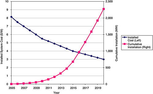
FIGURE D-7-2 An accelerated PV market development path for New York (all estimates are 2005 dollars).
TABLE D-7-4 Accelerated PV Deployment Scenario for New York (2005 dollars)
|
Year |
Annual Installations (MW) |
Growth Rate (%) |
Cumulative Installations (MW) |
Installed System Cost ($/W) |
Buydown Rate (%) |
Effective Buydown ($/W) |
Annual State Investment (million) |
Installed System Cost to Consumer ($/W) |
|
2005-actual |
2.0 |
NA |
4.2 |
8.14 |
52 |
4.23 |
8.47 |
3.91 |
|
2006 |
6.0 |
55 |
10.2 |
7.50 |
50 |
3.75 |
22.50 |
3.75 |
|
2007 |
9.3 |
55 |
19.5 |
7.00 |
45 |
3.15 |
29.30 |
3.85 |
|
2008 |
14.4 |
55 |
33.9 |
6.50 |
40 |
2.60 |
37.48 |
3.90 |
|
2009 |
22.3 |
55 |
56.3 |
6.00 |
35 |
2.10 |
46.92 |
3.90 |
|
2010 |
34.6 |
55 |
90.9 |
5.50 |
30 |
1.65 |
57.14 |
3.85 |
|
2011 |
53.7 |
40 |
144.6 |
5.20 |
25 |
1.30 |
69.78 |
3.90 |
|
2012 |
75.2 |
40 |
219.7 |
4.90 |
20 |
0.98 |
73.65 |
3.92 |
|
2013 |
105.2 |
40 |
324.9 |
4.60 |
15 |
0.69 |
72.60 |
3.91 |
|
2014 |
147.3 |
40 |
472.2 |
4.30 |
10 |
0.43 |
63.34 |
3.87 |
|
2015 |
206.2 |
40 |
678.4 |
4.00 |
5 |
0.20 |
41.24 |
3.80 |
|
2016 |
288.7 |
5 |
967.1 |
3.80 |
0 |
0.00 |
0.00 |
3.80 |
|
2017 |
303.1 |
5 |
1,270.3 |
3.60 |
0 |
0.00 |
0.00 |
3.60 |
|
2018 |
318.3 |
5 |
1,588.6 |
3.40 |
0 |
0.00 |
0.00 |
3.40 |
|
2019 |
334.2 |
5 |
1,922.8 |
3.20 |
0 |
0.00 |
0.00 |
3.20 |
|
2020 |
350.9 |
5 |
2,273.7 |
3.00 |
0 |
0.00 |
0.00 |
3.00 |
References
CLSA (Credit Lyonnais Securities Asia). 2004. Sun Screen: Investment Opportunities in Solar Power. CLSA Asia-Pacific Markets. Available at www.clsa.com.
DOE (Department of Energy). 2004. Solar Energy Technologies Program, Multi-Year Technical Plan 2003-2007 and Beyond. Office of Energy Efficiency and Renewable Energy, U.S. Department of Energy, Washington, D.C. Report DOE/GO-102004-1775.
DOE. 2005. Annual Energy Outlook 2005, Table 38. Energy Information Administration. Washington, D.C.
EC (European Commission). 2004. PV Status Report 2004: Research, Solar Cell Production and Market Implementation of Photovoltaics. European Commission, Directorate General Joint Research Centre, Renewable Energies Unit, Ispra, Italy. Report EUR 21390 EN.
EIA (Energy Information Administration). 2005. Electric Power Monthly. Energy Information Administration, U.S. Department of Energy, Washington, DC. (January).
EPA (Environmental Protection Agency). 2005. Control of Mercury Emissions from Coal Fired Electric Utility Boilers: An Update. Air Pollution Prevention and Control, U.S. EPA: Research Triangle Park, N.C.
EPIA (European Photovoltaic Industry Association). 2004. EPIA Roadmap. European Photovoltaic Industry Association, Brussels. Available at www.epia.org.
Ikki, Osamu. 2005. PV Activities in Japan. RTS Corporation, Tokyo, Japan (May).
Korens, N. 2002. Process Screening Analysis of Alternative Gas Treating and Sulfur Removal for Gasification. DOE/NETL: Pittsburgh.
Letendre, Steven, et al. 2003. “Solar And Power Markets: Peak Power Prices and PV Availability for the Summer of 2002.” Paper presented at ASES 2003, Austin, Tex., June.
Margolis, Robert M., and Frances Wood. 2004. “The Role for Solar in the Long-Term Outlook of Electric Power Generation in the U.S.” Paper presented at the IAEE North American Conference in Washington, D.C., July 8-10.
Navigant Consulting. 2004. PV Grid Connected Market Potential in 2010 Under a Cost Breakthrough Scenario. Report to the Energy Foundation. Available at www.navigantconsulting.com.
NEDO (New Energy and Industrial Technology Development Organization). 2004. PV Roadmap Toward 2030 (Japanese PV Industry Roadmap). New Energy and Industrial Technology Development Organization. Available at www.nedo.go.jp.
NYISO (New York Independent System Operator). 2005. “2004 Interim Review of Resource Adequacy Covering the New York Control Area for the Years 2004-2006.” January 24.
NYSERDA (New York State Energy Research and Development Authority). 2003. Energy Efficiency and Renewable Energy Resource Development Potential in New York State. New York State Energy Research and Development Authority, Albany, New York. Available at www.nyserda.org.
Oskarsson, K., Anders Berglund, Rolf Deling, Ulrika Snellman, Olle Stenback, and Jack Fritz. 1997. A Planner’s Guide for Selecting Clean-Coal Technologies for Power Plants. World Bank Technical Paper No. 387. Washington, D.C.: World Bank.
Parsons. 2002. The Cost of Mercury Removal in an IGCC Plant, P.I.a.T. Group, Editor.
Perez, Richard, et al. 2004a. “Quantifying Residential PV Economics in the US—Payback vs Cash Flow Determination of Fair Energy Value.” Solar Energy 77: 363-366.
Perez, Richard, et al. 2004b. “Solar Energy Security.” REFocus (July/ August): 24-29.
PowerClean, T.N. 2004. Fossil Fuel Power Generation State-of-the-Art, P.T. Network, Editor. University of Ulster: Coleraine, UK, pp. 9-10.
SEIA (Solar Energy Industries Association). 2004. Our Solar Power Future: The U.S. Photovoltaic Industry Roadmap Through 2030 and Beyond. Solar Energy Industries Association, Washington, D.C.
Strategies Unlimited. 2005. Personal Communication with Paula Mints, Senior Photovoltaic Analyst, Strategies Unlimited, Mountain View, California. February.
Thompson, J., 2005. Integrated Gasification Combined Cycle (IGCC)— Environmental Performance, in Platts IGCC Symposium. 2005: Pittsburgh.


