
3
Science Service Allocations
3.1
GENERAL CONSIDERATIONS
This chapter lists and discusses the science service spectrum allocations in the United States1 and their use. The Radio Regulations divides the world into three regions for spectrum allocation purposes. The United States is in Region 2 (see Figure 3.1).
3.1.1
Atmospheric Windows in the Radio Spectrum
The allocation of spectral bands for radio astronomy is based partly on the atmospheric windows available, as shown in Figure 3.2. Ground-based telescopes can observe only in the regions of the atmosphere that are not obscured. Below 50 GHz, there is a window between approximately 15 MHz and 50 GHz. Above 50 GHz, such radio windows occur at wavelengths around 3 mm (65-115 GHz), 2 mm (125-180 GHz), and 1.2 mm (200-300 GHz). At wavelengths shorter than 1 mm, the so-called submillimeter bands, the windows are less distinct, but clear ones exist at 0.8 mm (330-370 GHz), 0.6 mm (460-500 GHz), 0.4 mm (600-700 GHz), and 0.3 mm (800-900 GHz), as well as in other, smaller windows.
Furthermore, if Figure 3.2 showed absorption rather than transmission, the lines of particular importance to the Earth Exploration-Satellite Service (EESS) would be readily apparent: namely, the water lines at 22.235 and 183.1 GHz and the oxygen lines around 55-60 GHz and 118.75 GHz, as well as the available windows needed for comparison purposes, surface observations, and communications. Atmospheric absorption bands are used to measure atmospheric temperature and pressure profiles while using the windows to observe surface features, vegetation, and temperatures.
|
1 |
The U.S. and international spectrum allocation table and footnotes are available in the National Telecommunications and Information Administration’s Manual of Regulations and Procedures for Federal Radio Frequency Management (Redbook) at http://www.ntia.doc.gov/osmhome/redbook/redbook.html and in the Frequency Allocation Table at http://www.fcc.gov/oet/spectrum/table/. |
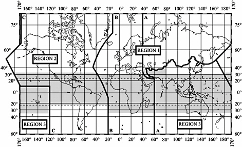
FIGURE 3.1 The regions as defined in Article 5 of the Radio Regulations. The shaded part represents the Tropical Zone. SOURCE: National Telecommunications and Information Administration, Manual of Regulations and Procedures for Federal Radio Frequency Management (Redbook), May 2003 edition, revised January 2006. See http://www.itu.int/ITU-R/ for more information.
3.1.2
Note to the Reader Regarding Frequency Allocation Tables
Because regulations, allocations, and footnotes can change, the reader is advised to consult the National Telecommunications and Information Administration’s (NTIA’s) Manual of Regulations and Procedures for Federal Radio Frequency Management (Redbook) or the Federal Communications Commission’s (FCC’s) FCC Online Table of Frequency Allocations, as well as the Radio Regulations, for the latest information. The Redbook can be found at http://www.ntia.doc.gov/osmhome/redbook/redbook.html, and the FCC’s document can be found at http://www.fcc.gov/oet/spectrum/table/fcctable.pdf. The information given in this chapter is current as of January 2006.
Each of the following eight sections in this chapter begins with a table of allocations for a specified frequency range—allocations below 1 GHz (Table 3.1), between 1 and 3 GHz (Table 3.2), between 3 and 10 GHz (Table 3.3), between 10 and 25 GHz (Table 3.4), between 25 and 50 GHz (Table 3.5), between 50 and 71 GHz (Table 3.6), between 71 and 126 GHz (Table 3.7), and between 125 and 275 GHz (Table 3.8).
The first column of each table lists the band allocations, and the fourth column elaborates on the scientific use of each band. In the second column, primary allocations are shown in capital letters (e.g., “RAS”), and secondary allocations appear in lowercase letters (e.g., “ras”). Footnotes to the tables indicate where the allocations in other regions differ. Parentheses around a science service—for ex-
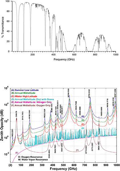
FIGURE 3.2 Top: Atmospheric windows in the radio spectrum commonly used in the Radio Astronomy Service community. The transmission is appropriate for a site of 400-m elevation and a precipitable water vapor content of 1 mm. Courtesy of Lucy Ziurys, University of Arizona. Bottom: Atmospheric zenith opacity in the radio spectrum commonly used in the Earth Exploration-Satellite Service community. From A.J. Gasiewski and M. Klein, “The Sensitivity of Millimeter and Sub-millimeter Frequencies to Atmospheric Temperature and Water Vapor Variations,” Journal of Geophysical Research-Atmospheres, Vol. 13, pp. 17481-17511, July 16, 2000.
ample, “(ras)”—indicate that one or more footnotes in the ITU Radio Regulations and/or the U.S. Table of Frequency Allocations provide limited protection.
Footnotes in the ITU Radio Regulations and the U.S. Table of Frequency Allocations that modify the allocations are noted in the third column of each table. A brief synopsis of each of these footnotes is given when it is first referenced in a table. Readers are advised to check for footnotes such as 5.340 and US211 that cover several bands.
Appendix I spells out the acronyms used in Tables 3.1 through 3.8 and describes the ITU Radio Regulations and the U.S. Table of Frequency Allocations footnote designations (e.g., for 5.350, US211, G59, and NG101).
3.2
ALLOCATIONS BELOW 1 GHZ
The bands, services, footnotes, and scientific observations for each band in the allocations below 1 GHz are presented in Table 3.1.
3.2.1
Solar Radio Bursts
Radio observations made at frequencies below ~100 MHz also capture data on solar bursts. Occasionally, and frequently during sunspot maximum, dramatic radio bursts of several different characteristic types are generated in the Sun’s atmosphere. Such bursts are sometimes associated with solar flares, which are sudden, violent explosions in the Sun’s chromosphere. The radio bursts are observed from ~20 to ~400 MHz and are more intense at the lower frequencies. The high-energy particles ejected from the Sun during these bursts may interact with Earth’s ionosphere and the stratosphere. Such interactions cause severe interruptions in radio communications and power systems and can also have dangerous effects on aircraft flights above 15 km. Studies of radio bursts aim to enable the prediction of failures in radio communications and the forecasting of other effects. Knowledge of the high-energy particle ejections from the Sun is essential for space exploration missions, both manned and unmanned. Continuous monitoring of the Sun’s activity will remain a high priority for the foreseeable future.
3.2.2
Jupiter Radio Bursts
Also significant is the peculiar nonthermal burstlike radiation from the giant planet Jupiter; this radiation is best observed at frequencies from ~15 to ~40 MHz. Extensive observations are being made at low frequencies in order to study this unusual radiation. It was observed by the Voyager spacecraft, but further ground-based studies are essential.
3.2.3
Interstellar Medium
The low-frequency range below 1 GHz also has a great importance in the observations of both the thermal and nonthermal diffuse radiation in our own Milky Way Galaxy. Such galactic observations give information about the high-energy cosmic ray particles in our Galaxy and about their distribution, and also about the hot ionized plasma and star birth in the disk of our spiral Galaxy. In particular, the ionized interstellar clouds can be studied at low frequencies where the sources are opaque and their spectra approximate the Planck thermal radiation (blackbody) law. Such spectral observations can be used directly to measure the physical parameters of the radiating clouds, particularly their temperatures.
TABLE 3.1 Frequency Allocations Below 1 GHz: Bands, Services, Footnotes, and Scientific Observations
|
Band (MHz) |
Services |
Footnotes |
Scientific Observations |
|
13.36-13.41 |
RAS, FS1 |
Sun, Jupiter, interstellar medium, steep spectrum sources |
|
|
25.55-25.67 |
RAS |
5.149, US74,4 US342 |
Sun, Jupiter, interstellar medium, steep spectrum sources |
|
37.50-38.25 |
FS, MS, ras5 |
Sun, Jupiter, interstellar medium, steep spectrum sources |
|
|
73.00-74.60 |
5.178,11 US74 |
Sun, interstellar medium, steep spectrum sources |
|
|
137-138 |
SO, MetSat, SRS, MS12 |
5.204, 5.205, 5.206, 5.207, 5.208, US319, US230 |
NOAA (EESS) communications bands |
|
150.05-153.0 |
5.149, 5.208A16 |
Sun, interstellar medium, steep spectrum sources, pulsars, continuum (single-dish mode) |
|
|
322.0-328.6 |
RAS, FS, MS |
Deuterium, Sun, interstellar medium, steep spectrum sources, pulsars |
|
|
400-406 |
MetAids (radiosonde), MetSat (S→ E), MS (S→ E), SRS (S→ E), MS (S→ E), EESS (E→ S) See NTIA Redbook |
5.263, 5.264, US70, US329, US320, US324 |
NOAA (EESS) communications bands |
|
406.1-410 |
RAS, FS, MS |
Sun, interstellar medium, steep spectrum sources, pulsars |
|
|
432-438 |
eess (active) |
5.279A |
Biomass and soil measurements |
|
460-470 |
See NTIA Redbook |
|
NOAA (EESS) communications bands |
|
608-614 |
5.149, 5.208A, US74, US24625 |
Sun, interstellar medium, steep spectrum sources, pulsars |
Several hundred such galactic clouds appear approximately as blackbodies at frequencies below ~100 MHz.
The recombination lines that occur in this frequency range arise from very high energy levels, in which the electron orbits very far from the nucleus. In fact, these atoms are so large that the orbits of the outer electrons are affected by the electrons of other atoms in a measurable way, serving as a probe of the density of the gas. Recombination lines are further described in §3.3.8.
3.2.4
Deuterium
The frequency range 322-328.6 MHz contains the hyperfine-structure spectral line of deuterium at 327.384 MHz. The study of this line has impacts on problems related to the origin of the universe and the cosmological synthesis of the elements. The recent detection of deuterium emission in the outer region of our Galaxy required months of integration time, with careful attention to mitigation of radio-frequency interference. Continuing study of the deuterium abundance in other parts of our Galaxy can further refine our understanding of the early universe.
|
NOTE: For definitions of acronyms and abbreviations, see Appendix I. For information about other features of this table, see §3.1.2, “Note to the Reader Regarding Frequency Allocation Tables.” 1Not in the United States. 2ITU RR footnote 5.149 urges administrations to take all practical steps to protect the RAS from other services in this band. 3U.S. (federal government services) footnote G115 limits protection for national defense and emergency needs. 4U.S. (all services) footnote US74 limits protection from transmitters in other bands. 5Primary in the United States from 38.00-38.25 MHz. 6US81 authorizes limited military use in the 38.00-38.25 MHz band. 7NG59 authorizes use of the 37.60-37.85 MHz band by power service utilities. 8NG124 authorizes low-power police radio on a non-interference basis. 9In Regions 1 and 3. 10In Regions 1 and 3. 11Additional allocation in some Caribbean nations to the fixed and mobile services on a secondary basis. 12MS is secondary in 137.025-137.175 MHz and 137.825-138.0 MHz. 13In Region 1. 14Except aeronautical. 15In Region 2, by S5.149. 165.208A provides footnote protection from space transmitters outside the band. 17G27 limits the FS and MS to military use. 18See G100 in Appendix B.3. 19G5 authorizes FS and MS for government nonmilitary agencies only. 20G6 allows military operations subject to local coordination. 21US117 limits transmitter power. 22US13 authorizes hydrological and meteorological fixed stations at specific frequencies. 23Footnote protection only in Regions 1 and 3. 24Except aeronautical; Earth-to-space only. 25US246 prohibits transmissions. |
3.2.5
Steep-Spectrum Continuum Sources
Most radio sources (such as radio galaxies, quasars, and supernova remnants) have characteristic nonthermal spectra produced by synchrotron emission from relativistic cosmic ray electrons moving in galactic-scale magnetic fields. As shown in Figures 2.1 and 2.2 in Chapter 2, these nonthermal sources typically have radio spectra with negative slopes of ~0.8 in a graph of log (flux density) versus log (frequency). Hence, such sources have higher radio flux densities at lower frequencies.
The steepness of the spectrum depends on the energy of the electrons. As synchrotron sources age, the most energetic electrons are lost and the spectra steepen with time.
At longer wavelengths, the spiraling electrons have increasingly higher cross sections for absorbing radiation, so that the emitted radiation is increasingly likely to be reabsorbed before escaping from the region. This causes turnovers in the spectra at low frequencies (see Figures 2.1 and 2.2), and the frequencies at which they occur are diagnostics of the emitting region.
The low-frequency part of the spectrum is also where one finds the emission from highly redshifted radio sources, those that exist in the most distant parts of the universe.
The Arecibo Telescope in Puerto Rico, The Green Bank Telescope in West Virginia, the Very Large Array in the state of New Mexico, and the Very Long Baseline Array (VLBA)—a system of 10 radio telescope antennas positioned from Hawaii to the U.S. Virgin Islands—operate in these bands, as well as the Giant Metrewave Radio Telescope (GMRT) in India and the Westerbork Array in the Netherlands.
High-resolution observations of radio galaxies and quasars have also been made with the GMRT using the method of lunar occultations, which uses the lunar disk to eclipse distant radio sources as they move across the sky. From such occultations, it has been possible to determine the shapes and positions of many extragalactic radio sources with very high accuracies, on the order of 1 arc second.
3.2.6
Pulsars
One of the most interesting and significant discoveries in radio astronomy has been the detection of pulsars, for which Antony Hewish was awarded the Nobel Prize in physics in 1974. The understanding of stellar evolution has been advanced by providing a method of studying these rapidly rotating, highly magnetized neutron stars. Pulsars’ extreme magnetic, electric, and gravitational fields, impossible to reproduce in laboratories on Earth, allow observations of matter and radiation under such conditions. Pulsars now provide the most accurate timekeeping, surpassing the world’s ensemble of atomic clocks for long-term time stability.
Pulsars are understood to be highly condensed neutron stars that rotate with a period as short as a millisecond. Such objects are produced by the collapse of the cores of massive stars during the catastrophic explosions known as supernova outbursts. The radio spectra of pulsars indicate a nonthermal mechanism, perhaps of synchrotron emission type. Observations have shown that the pulsars emit strongest at frequencies in the range from ~50 to 600 MHz. Hence, many observations are being performed at such frequencies. However, important observations and surveys are being conducted at frequencies up to 10 GHz.
The discovery and the study of pulsars during the past two decades have opened up a major new chapter in the physics of highly condensed matter. The study of neutron stars with densities on the order of 1014 g/cm3 and with magnetic-field strengths of 1012 gauss has already contributed immensely to our understanding of the final stages of stellar evolution and has brought us closer to understanding black holes (which are thought to be the most highly condensed objects in the universe). Low-frequency bands 6-8 GHz are indeed important for pulsar observations, but exclusive bands in this range are not allocated.
The Nobel Prize in physics in 1993 was awarded to Russell A. Hulse and Joseph H. Taylor, Jr., “for the discovery of a new type of pulsar, a discovery that has opened up new possibilities for the study of gravitation.”2 Binary pulsars have provided the best experimental tests of predictions of the theory of general relativity and strong evidence for the existence of gravitational radiation.
Careful analysis of pulse timing residuals led to the startling discovery by radio astronomers Aleksander Wolszczan and Dale Frail in 1991, and confirmed in 1994, that pulsars can have planetsized bodies in orbit around them—the first detection of extrasolar planets. Pulsars are also diagnostics of the interstellar medium’s density and magnetic field. Continuum bands, particularly those at frequencies below 3 GHz, are most valuable for these studies.
|
2 |
Located at http://nobelprize.org/nobel_prizes/physics/laureates/1993/press.html, accessed September 14, 2006. |
3.3
BANDS BETWEEN 1 AND 3 GHZ
In addition to the bands listed in Table 3.2, scientific use is also made of the 1675-1690 MHz Meteorological Aids Service (MetAids) band; the 1215-1300 MHz EESS active band, which is used for synthetic aperture radar (SAR) missions; and the Global Positioning System (GPS) bands at 960-1215 MHz, 1215-1300 MHz, and 1559-1610 MHz.
3.3.1
Neutral Atomic Hydrogen
One of the most important spectral lines at radio wavelengths is the 21 cm line (1420.406 MHz), corresponding to the F = 1 → 0 hyperfine transition of neutral atomic hydrogen (HI). Radio observations of this line have been used since its discovery in 1951 to study the structure of our Galaxy and those of other galaxies. Because of Doppler shifts owing to the distance and motion of the hydrogen clouds that emit this radiation, the frequency for observing this line emission ranges from below 1 GHz to ~1430 MHz. Numerous and detailed studies are being made of the HI distribution in our Galaxy and in other galaxies. Such studies are being used to investigate the state of cold interstellar matter; the dynamics, kinematics, and distribution of the gas; the rotation of our Galaxy and of other galaxies; and the masses of other galaxies.
The HI emission is relatively strong and, with current receiver sensitivity, such emission is detectable from any direction in our Galaxy and from a very large percentage of the nearby galaxies. The 1330-1400 MHz band is important for observations of redshifted HI gas from distant external galaxies. Such observations of redshifted HI have been made in a quasi-continuous range of frequencies down to 1260 MHz. Below this frequency, detections have been made at individual, isolated frequencies. Observations of HI below 1330 MHz have been limited in the past by spectrometer bandwidths, dynamic range, and limitations of sampling (dump time). Studies of the evolution of the HI mass function with cosmic time will require observations below 1260 MHz and are being proposed for systematic and concerted studies. As radio telescopes become more powerful, it will be possible to detect more-distant, and therefore more-redshifted (and therefore younger) galaxies. This increase in capability will allow astronomers to study how galaxies evolve.
3.3.2
Lines of Hydroxyl
The study of hydroxyl (OH) is of great interest for investigating the physical phenomena associated with the formation of protostars and the initial stages of star formation.
3.3.2.1
Thermal Emission
The OH molecule has been observed widely in our Galaxy in the four hyperfine components of the ground-state lambda-doubling transitions at 1665, 1667, 1612, and 1720 MHz. OH has been detected in thermal emission and absorption in several hundred different molecular complexes in our Galaxy.
Thermal OH emission, which predominates in the low-density envelopes of molecular clouds, is the principal means for studying these envelopes. In addition, the two oppositely circularly polarized components become slightly separated in frequency in the presence of a magnetic field. This so-called Zeeman effect is the only way to measure the strength of the magnetic field in these regions. The magnetic field may play a major role in the dynamics of the gas.
TABLE 3.2 Frequency Allocations Between 1 and 3 GHz: Bands, Services, Footnotes, and Scientific Uses
|
Band (MHz) |
Services |
Footnotes |
Scientific Use |
|
1300-1350 |
AeRNS,1 rls, (ras) |
Extragalactic HI,5 recombination lines |
|
|
1350-1400 |
5.149, 5.334,13 5.338,14 5.339,15 US311,16 US350,17 US351,18 G2, G27,19 G11420 |
Extragalactic HI, recombination lines |
|
|
1400-1427 |
RAS, EESS (passive), SRS (passive) |
Galactic and local extragalactic HI, recombination lines, radio source spectra, galactic continuum |
|
|
1559-1610 |
AeRNS, RNSS (S→ E) and (S→ S) |
Extragalactic OH masers |
|
|
1610-1610.6 |
MSS (E→ S), AeRNS, RDSS (E→ S),26 (ras) |
5.341, 5.355, 5.359, 5.363,27 5.364,28 5.367,29 5.370,30 5.371,31 5.372,32 US208,33 US260,34 US31935 |
Extragalactic OH |
|
1610.6-1613.8 |
RAS, MSS (E→ S), AeRNS, RDSS (E→ S)36 |
5.149, 5.341, 5.355, 5.359, 5.363, 5.364, 5.367, 5.369, 5.370, 5.371, 5.372, US319 |
OH |
|
1660-1660.5 |
MSS (E→ S), RAS |
OH |
|
|
1660.5-1668.4 |
RAS, SRS (passive), fs, ms (except aems) |
OH |
|
|
1668.4-1670 |
5.149, 5.341, US74, US9946 |
OH |
|
|
1670-167547 |
5.341, US21151 |
OH |
|
|
1690-1700 |
MetAids,52 MetSat (S→ E),53 MSS (E→ S),54 fs,55 ms (except Ae),56 (eess) |
|
|
|
1700-1710 |
|
||
|
1718.8- 1722.263 |
FS, MS, ras |
OH |
|
|
2025-2110 |
|
||
|
2110-212074 |
FS, MS, SRS (deep S→ E) |
US25275 |
|
|
2200-2290 |
SRS (deep S→ E, S→ S), EESS (S→ E, S→ S), FS,76 MS,77 SRS (S→ E, S→ S) |
Deep space downlinks, VLBI |
|
|
2290-2300 |
FS, MS, SRS81 |
|
|
|
2310-2360 |
ms, rls, fs, BS |
US33882 |
Radar astronomy83 |
|
2640-2655 |
srs (passive), eess (passive), FS, MS, FSS, BSS |
5.33984 |
Extragalactic radio sources, galactic continuum |
|
Band (MHz) |
Services |
Footnotes |
Scientific Use |
|
2655-2690 |
ras, srs (passive), eess (passive), FS, FSS,85 MS, BSS, MSS |
|
|
|
2690-2700 |
RAS, EESS (passive), SRS (passive) |
5.340, 5.413,91 US74, US246 |
|
|
NOTE: For definitions of acronyms and abbreviations, see Appendix I. For information about other features of this table, see §3.1.2, “Note to the Reader Regarding Frequency Allocation Tables.” 1In the United States only. 25.149 urges administrations to take all practical steps to protect the RAS from other services using the band 1330-1400 MHz. 35.337 limits ANS to ground-based radars and airborne transponders activated by these radars. 4Government radiolocation is limited to the military services. 5HI, neutral atomic hydrogen. 6In Region 1 only. 7Secondary from 1390 to 1395 MHz and no allocation from 1395 to 1400 MHz in the United States. 8In Region 1 only. 9Secondary from 1390 to 1395 MHz and no allocation from 1395 to 1400 MHz in the United States. 10In the United States only from 1395 to 1400 MHz. 111370-1400 MHz only. 121370-1400 MHz only. 135.334, in Canada and the United States, adds the Aeronautical Radionavigation Service on a primary basis between 1350 and 1370 MHz. 145.338 allows existing installations of the radionavigation service in certain countries in eastern Europe to continue to operate in the band 1350-1400 MHz. 155.339 authorizes passive EESS and SRS in the 1370-1400 MHz band. 16US311 provides partial geographic protection only from 1350 to 1400 MHz. 17US350: LMS is limited to medical telemetry and telecommand operations. 18US351: Government operations are on a noninterference basis with nongovernment operations. 19G27 limits the FS and MS to military use. 20G114 authorizes space-to-Earth relay of nuclear burst data by the FSS and MSS in the 1369.05-1381.05 MHz band. 215.340 prohibits all emissions in this band. 225.341 makes note of SETI. 235.355 adds FS on a secondary basis in certain countries. 245.359 adds FS on a primary basis in certain counties but urges administrations to make no additional allocations. 25G126 allows addition of differential GPS on a primary basis. 26Primary in Region 2, secondary in Region 3, not in Region 1. 275.363 adds AeRNS on a primary basis in Sweden. 285.364 limits transmitter power and requires coordination. 295.367 adds AeMS(route) on a primary basis. 305.370: RDSS is secondary in Venezuela. 315.371 adds RDSS on a secondary basis in Region 1. 325.372 protects the RAS in the band 1610.6-1613.8 MHz from the RDSS and MSS. 33US208 states that sharing criteria and techniques need to be developed. 34US260 authorizes AeMS when it is an integral part of the ARS. 35US319 limits federal government use. 365.364 limits transmitter power and requires coordination. 375.149 urges protection of RAS when making assignments to other services in the band 1660-1670 MHz. 385.351 forbids feeder links. 395.376A protects the RAS from the MSS Earth stations. 405.379 provides additional secondary allocation to MetAids in certain countries. 415.379A urges further protection to the RAS in the 1660.5-1668.4 MHz band. 42US74 limits the protection to the RAS. |
|||
Emission lines from 18OH and 17OH have been detected in some molecular regions of our Galaxy. The data from these lines allow the study of the abundances of the oxygen isotopes involved. Such studies are a crucial part of understanding the network of chemical reactions involved in the formation of atoms and molecules. The data can help astronomers to understand the physics of stellar interiors, the chemistry of the interstellar medium, and the physics of the early universe.
3.3.2.2
Maser Emission
Extremely narrow and intense emission lines of OH have been seen in certain galactic regions. This emission is due to maser action and can be associated with star-forming regions and with more-evolved stars. Observations of OH maser sources using the powerful technique of very long baseline interferometry (VLBI) have shown that the masing regions have apparent angular sizes on the order of 0.01 arc second or less. Such apparent sizes translate to linear sizes on the order of a few times the mean distance between Earth and the Sun (150 million km) and occur at the heart of regions with active star formation.
The 1612 MHz transition is an extremely important hyperfine line of OH. This line emission occurs in many types of objects in the Galaxy, and high-angular-resolution observations of these objects in this line measure their distances and can be used collectively to measure the distance to the center of the Galaxy.
3.3.2.3
Extragalactic Megamasers
OH can be seen in other galaxies by absorption against radio sources in galactic nuclei and by maser emission. The OH megamaser emission from galactic nuclei can be more than a million times more luminous than that from galactic masers and can be seen to great distances. The present redshift limit for extragalactic masers is 50,000 km/s (z = 0.17), which causes the OH line to be observed at 1428 MHz. These powerful megamasers arise within the cores of galaxies; this action results in amplification (rather than absorption) of the nuclear radio continuum. Use of the OH line to study these very peculiar and active galaxies allows radio astronomers to diagnose the temperature and density of the molecular gas in the centers of these galaxies.
3.3.3
Extragalactic Radio Source Spectra
The study of the continuum emission of radio sources requires observations throughout a very wide frequency range. The 1-3 GHz bands (at 1400-1427 MHz, 2200-2300 MHz, and 2655-2700 MHz) are important for continuum observations to determine the physical parameters in a wide variety of radio sources (Figures 2.1 and 2.2 in Chapter 2). Many extragalactic radio sources show a “break” in their nonthermal spectrum in the region between 1 and 3 GHz; continuum measurements in the range of 2 to 3 GHz are essential to define such a spectral characteristic accurately. The spectral break at relatively high frequencies from synchrotron sources is closely related to the lifetime of relativistic particles in radio galaxies and quasars. Such information is crucial to our understanding of the physical processes taking place in radio sources.
3.3.4
Galactic Continuum
The frequency bands in the range from 1 to 3 GHz are also important for galactic studies of ionized hydrogen clouds and the general diffuse radiation of the Galaxy. Since, at such frequencies, available
radio telescopes have adequate angular resolution (narrow beams, of the order of 10 arc minutes [arcmin] for large telescopes), many useful surveys of the galactic plane have been performed, including the regions of the galactic center, which is invisible at optical wavelengths because of the interstellar absorption by dust particles.
The Arecibo Observatory’s telescope, with a beam of 3.3 arcmin, will soon begin surveying the galactic continuum (at a resolution of better than 10 arcmin) to study the galactic magnetic field. The most serious hindrance to full exploitation of existing cosmic microwave background (CMB) data sets, including those from the Wilkinson Microwave Anisotropy Probe (WMAP) and future data sets from the Planck mission and other future missions, is the understanding of the galactic foreground, especially at the frequencies used for CMB experiments (20-100 GHz). It is thus imperative that detailed studies of the galactic continuum emission be undertaken.
3.3.5
Very Long Baseline Interferometry
Because of the sensitive, large antennas of the NASA Deep Space Network and other deep space stations, the 2290-2300 MHz band allocated to the Space Research Service (SRS) is also used for VLBI observations in radio astronomy. The 2200-2290 MHz band is widely used in conjunction with the SRS band just above it. In particular, major geodetic and astrometric programs are being carried out jointly in the 2200-2300 MHz frequency range.
The study of the nuclei of galaxies, including that of our own Galaxy, is emerging as an extremely important and fundamental topic in astronomy. Problems that can be studied in these objects include the state of matter and the possibility of the existence of black holes in galactic nuclei, the explosive activities and the production of intense double radio sources from galactic nuclei, the influence of galactic nuclei on the morphological structure of galaxies, the formation of galaxies and quasars, and many other relevant and major astrophysical topics.
The center of our Galaxy is perhaps its most interesting region, but it can be observed only at infrared and radio wavelengths, since such long wavelengths are not affected by the dust particles in interstellar space. Because of this use by radio astronomers, many radio telescopes are equipped to use this band, which in turn allows radio telescopes to support important space missions.
Continuum observations in several discrete channels spanning over 100 MHz around 2300 MHz and spanning 500 MHz or more around 8600 MHz are used for high-precision position measurements, important for both radio astronomy and the Earth sciences. Although it is not possible to make such precise measurements using only bands allocated to the passive services, these measurements are possible because some interference can be tolerated at some of the antennas part of the time. However, the recent activation of broadcast satellites in the 2300 MHz band is making these measurements more difficult. The broadcast satellites and other sources of interference may make it necessary to move geodetic observations to the 31 GHz band, where 500 MHz is protected for radio astronomy and other passive services.
3.3.6
Astronomical Polarization Studies
An important study at radio wavelengths is the polarization of the radiation that is observed from radio sources. Radio sources are often found to be weakly linearly polarized, with a polarization angle that depends on frequency. This effect is due to the fact that the propagation medium in which the radio waves travel to reach us is composed of charged particles, electrons, and protons, in the presence of magnetic fields. The determination of the degree and angle of polarization gives us information on the
magnetic fields and electron densities of the interstellar medium, and in certain cases on the nature of the emitting sources themselves. The degree of polarization of radio waves is higher at higher frequencies. The frequency bands near 2300, 2700, and 5000 MHz are important bands for polarization measurements.
3.3.7
Soil Moisture
A combination of active and/or passive microwave measurements can be used to remotely sense soil moisture under moderately vegetated areas (up to ~5 kg/m2 of vegetation water content) with an uncertainty of approximately 4 percent volumetric soil moisture. Passive measures rely on the dependence of the microwave emissivity of soil to its water content, but passive measures are complicated by surface roughness. Lower microwave frequencies provide good soil penetration depth, permitting measurements of soil moisture down to ~10 cm depth at 1.4 GHz, and less so at higher frequencies. Active measurements rely on the dependence of soil backscatter on water content and are complicated by surface roughness and scattering by vegetation cover. While passive techniques have a strong two-decade development heritage, active measurements can, however, provide finer spatial resolution than is possible with passive techniques. Thus, a combination of active and passive measurements can be used to separate the effects of surface roughness and vegetation scattering from the soil-moisture signature while providing the desired spatial resolution.
Soil moisture is a key component of the land-surface hydrospheric state. It is essential to estimating latent heat and carbon fluxes at the land-atmosphere boundary. These quantities are vital to weather and climate prediction and research.
3.3.8
Recombination Lines
After an atom is ionized, the nucleus eventually recaptures an electron, which then cascades down through a series of energy levels, emitting narrow spectral line radiation. Such lines occur throughout the spectrum and serve as probes of the temperature and density of nebulae surrounding newly formed stars and the extended envelopes of certain late-type stars.
The physics of the ionized hot gaseous clouds between the stars has been studied by observations of radio lines of excited hydrogen, helium, and carbon. Some of these studies have been made at frequencies of 1399 and 1424 MHz. Detailed observations of radio recombination lines in many interstellar clouds have made possible the derivation of physical parameters such as temperature, density, and velocity distributions. Radio studies have been particularly helpful for observations of these clouds, which are partially or totally obscured at optical wavelengths by interstellar dust.
3.3.9
Radar Astronomy
The Arecibo Observatory in Puerto Rico and the NASA Goldstone 70 m antenna in California have powerful radar transmitters that are used to study objects in the solar system as far away as Saturn. Mercury, Venus, the Moon, Mars, and the satellites of Jupiter and Saturn (including the rings of Saturn) are all objects of study. Comets and asteroids, particularly those that pass near to Earth, are routine targets of these radars.
Although the transmitters are very powerful, about 500 kW, the returned signals are extremely weak and vulnerable to interference. The radar frequency 2320 MHz is close to powerful broadcast satellite transmissions near 2330 MHz, which is a great concern. This panel also notes the importance of bistatic
radar and radar interferometry for the study of the most-distant bodies but also of near-Earth asteroids, including potentially dangerous ones. Another important use of radio astronomy telescopes is for ground-based telemetry for space missions (e.g., the Cassini mission used Very Long Baseline Array during the descent of the Huygens probe at Titan, and the Green Bank Telescope acquired signals from the probe).
3.3.10
Sea-Surface Salinity
The emissivity of seawater below 3 GHz is affected by its near-surface salinity. Monthly averaged global maps of salinity with 0.1-0.2 part-per-thousand sensitivity are theoretically possible at 1.4 GHz. The emissivity, however, is also affected by the sea-surface roughness. Thus, active microwave measurements near 1.3 GHz utilizing a radar scatterometer are needed in combination with passive measurements to correct the radiometer brightness temperatures and thus estimate surface salinity at sensitivities approaching the theoretical precision.
Monthly global maps of sea-surface salinity (SSS) would complement sparsely sampled in situ measurements of SSS from ships and ocean buoys. When combined with available global sea-surface temperature data, the improved SSS measurements would greatly improve models of density-driven ocean circulation and could be used to develop a significantly better understanding of heat flux at the sea surface for coupled ocean-atmosphere climate models. Ocean circulation is largely responsible for oceanic heat transport, which in turn strongly influences climate and is suspected of influencing the intensity and frequency of hurricanes. Coupled ocean-atmosphere models are used for the study of natural climate variability and for understanding and predicting climate changes. Remotely sensed salinity measurements are also valuable for understanding sea-ice melting and freezing processes; improved discrimination between meltponds, sea-ice leads, and polynia; and littoral and estuarine biological blooms and their impact on primary production and the health of fisheries.
3.4
BANDS BETWEEN 3 AND 10 GHZ
In addition to the bands listed in Table 3.3, the following bands are used for scientific research: the EESS active (secondary) band at 3.1-3.3 GHz, the Meteorological Satellite Service (MetSat) radar EESS active (secondary) band at 9.975-10.025 GHz, the EESS active bands at 17.20-17.30 GHz and (secondary) 24.05-24.25 GHz, and the EESS passive (secondary) band at 4.200-4.400 GHz.
An EESS passive (secondary) band runs from 4.90 to 5.00 GHz. The SRS Earth-to-space communication band is 7.145-7.235 GHz. Additional (MetSat) communication bands are 7.450-7.55 GHz (geostationary) and 7.55-7.85 GHz (low-Earth orbiters). Note that some of these allocations may be difficult to find in the regulatory footnotes.
3.4.1
Formaldehyde
Formaldehyde (H2CO) is detected in interstellar clouds via its K-doubling transition (JK−1,K+1 = 110-111) at 4829.66 MHz. This line is a useful tracer of the more diffuse interstellar medium because it can be detected in absorption against strong background radio sources. The distribution of H2CO clouds can give independent evidence of the distribution of the interstellar material and can help in understanding the structure of our Galaxy. H2CO lines from the carbon-13 isotope and oxygen-18 isotope have been detected, and studies of the isotopic abundances of these elements are being carried out.
TABLE 3.3 Frequency Allocations Between 3 and 10 GHz: Bands, Services, Footnotes, and Scientific Uses
|
Band (MHz) |
Services |
Footnotes |
Scientific Use |
|
3260-3267 |
RLS, (ras) |
CH |
|
|
3332-3339 |
5.149, G317 |
|
|
|
3345.8-3352.5 |
5.149, G31 |
|
|
|
4800-4990 |
FS, MS, ras, eess (passive), srs (passive) |
Formaldehyde, continuum |
|
|
4990-5000 |
RAS, FS, MS,16 srs (passive) |
Continuum, VLBI |
|
|
5250-5255 |
EESS (active), RLS, SRS (active) |
5.448A21 |
|
|
5255-5350 |
EESS (active), AeRNS, rls |
|
|
|
5350-5460 |
EESS (active), AeRNS |
5.449 |
|
|
5660-5725 |
RLS, aems, srs (deep space) |
5.45424 |
|
|
6425-6650 |
FS, FSS, MS, (eess passive), (srs passive) |
5.45825 |
Passive remote sensing |
|
6650-6675.2 |
FS, FSS (E→ S), MS, (eess passive), (srs passive), (ras) |
5.149,26 5.458 |
Methanol, passive remote sensing |
|
6675.2-6700 |
FS, FSS (E→ S), MS, (eess passive), (srs passive) |
5.458 |
Passive remote sensing |
|
6700-7075 |
FS, FSS, MS, (eess passive), (srs passive) |
|
|
|
7075-7125 |
FS, MS, (eess passive), (srs passive) |
|
|
|
7125-7190 |
FS, MS,27 (eess passive), (srs passive) |
|
|
|
7190-7235 |
FS, MS,28 SRS (E→ S), (eess passive), (srs passive) |
5.458 |
Deep space uplinks, passive remote sensing |
|
7235-7250 |
FS, MS,29 (eess passive), (srs passive) |
5.458 |
Passive remote sensing |
|
8025-8175 |
|
||
|
8175-8215 |
EESS (S→ E), FS, FSS (S→ E), MetSat (E→ S), MS |
5.462A, 5.463 |
|
|
8215-8400 |
EESS (S→ E), FS, FSS (E→ S), MS |
5.462A, 5.463 |
|
|
8400-8450 |
Deep space downlinks, continuum, VLBI |
||
|
8450-8500 |
SRS (S→ E) |
5.466 |
Continuum, VLBI |
|
8500-8550 |
RLS |
Radar astronomy |
|
|
8550-8650 |
EESS (active), RLS, SRS (active) |
5.468, 5.469, 5.469A40 |
|
|
9500-9800 |
EESS (active), RLS, RNS, SRS (active) |
||
|
NOTE: For definitions of acronyms and abbreviations, see Appendix I. For information about other features of this table, see §3.1.2, “Note to the Reader Regarding Frequency Allocation Tables.” |
|||
The combination of the 4830 MHz and 14.5 GHz formaldehyde lines is a sensitive and useful diagnostic of the density in the emitting gas.
Extragalactic formaldehyde megamaser emission and absorption are found in a growing number of galaxies. Since formaldehyde is a good tracer of intermediate- to high-density gas, this line is very important for the study of the molecular structure of other galaxies.
3.4.2
Continuum and Very Long Baseline Interferometry
The spectral band around 5 GHz has been one of the most widely used frequency ranges in radio astronomy during the past decade. Astronomers have made use of this frequency range in order to study
the detailed brightness distributions of both galactic and extragalactic objects. Detailed radio maps of interstellar ionized hydrogen clouds and supernova remnants have assisted our understanding of the nature of such celestial objects. These radio maps define the extent and detailed morphology of radio sources and enable us to make conclusions concerning their structures and dynamics and to derive physical parameters of the sources such as their total masses.
Heavy use has been made of the radio astronomy band at 5 GHz for VLBI observations. Angular resolutions of 0.3 milliarc seconds have been achieved with intercontinental baselines, and many countries (Australia, Canada, Germany, Great Britain, The Netherlands, Russia, South Africa, Spain, and Sweden) have collaborated in this effort. From such studies, astronomers are finding that quasars are composed of intricate structures with many strong localized sources of radio emission.
The 8400-8500 MHz band is widely used for VLBI studies in conjunction with and in support of geodetics and space research (space-to-Earth) experiments.
3.4.3
Soil Moisture
Passive microwave measurements in the C-band region, typically near 6.8 GHz, can be used to infer soil moisture in the surface layer (typically 0-1 cm) under bare soil and lightly vegetated areas (up to ~2 kg/m2) to approximately 10 percent volumetric accuracy. Applications are discussed in §3.3.7.
3.4.4
Sea-Surface Temperature
The brightness temperature of the sea surface is dependent on the thermometric sea-surface temperature (SST), the salinity, and surface roughness and foam. Observation at frequencies above ~5 GHz ensures minimal dependency on sea-surface salinity, and observation below ~10 GHz reduces the effect of roughness, ocean foam, and clouds while maintaining sensitivity to SST, especially in colder regions. An optimal spectral region to determine SST using microwave radiometry is thus near ~6 GHz, although no EESS allocation currently exists near this frequency.
Sea-surface temperature measurements of ~0.3°C precision or better are possible from spaceborne radiometers operating near ~6.8 GHz with 100-400 MHz bandwidth. Estimates of SST based on microwave radiometric measurements over the ocean at this frequency are largely immune to cloud cover, which strongly inhibits thermal infrared (IR) measurements. Microwave SST measurements are also complementary to IR measurements in providing SST data more representative of the bulk water temperature rather than of the thin infrared skin-depth layer. When combined, IR and microwave SST measurements can potentially provide measurements of the heat flux from the ocean surface.
SST data are used to support studies of a broad range of sea-surface phenomenology, climate studies, and weather forecasting. For example, the strengthening of hurricanes and cyclones strongly depends on oceanic heat content, which is directly related to SST. In general, climate studies require only relatively coarse spatial resolution (~25 km) but measurements under all cloud conditions. Accurate microwave measurements thus play a significant role in providing input SST data for numerical climate models.
3.4.5
Microwave Radiometric Imagery
See § 3.5.13 for applications of microwave radiometric imagery.
3.5
BANDS BETWEEN 10 AND 25 GHZ
The bands, services, footnotes, and scientific observations for each band in the allocations between 10 and 25 GHz are presented in Table 3.4.
3.5.1
Very Long Baseline Interferometry
Many of the nonthermal synchrotron sources are only detectable at higher frequencies, and the frequency range of 10-25 GHz gives us such observational information. This frequency range is also important for monitoring the intensity variability of the quasars. These objects, which could be the most-distant celestial objects that astronomers can detect and which produce surprisingly large amounts of energy, have been found to vary in intensity over periods of weeks and months. Such observations lead researchers to estimate the sizes of these sources, which turn out to be very small for the amount of energy they produce. The variability of quasars (and some peculiar galaxies) is more pronounced at higher frequencies; observations at these frequencies facilitate the discovery and the monitoring of these events. The energy emitted during any one such burst from a quasar is equivalent to the complete destruction of a few hundred million stars in a period of a few weeks or months. Astronomers do not yet understand the fundamental physics that can produce such events. Observations of the size and variability of these sources are the primary means that can be used to determine their nature. These observations are now best performed in the frequency range from 10 to 15 GHz.
The small sizes of the quasars are revealed from the VLBI observations mentioned above. Such observations are also being made in the frequency band at 10.6-10.7 GHz, and observations at 15.40 GHz have been successful. The higher frequencies provide better angular resolutions and enable more accurate determination of the sizes and structures of quasars.
3.5.2
Precipitation Measurements
Precipitation measurements using microwave remote sensing may utilize both active and passive sensing. Rain mapping using radar reveals the three-dimensional structure of precipitation, which can be used to develop statistical cloud and raincell models and to provide improved calibration of rainfall measurements derived using passive radiometry alone. Microwave radiometric measurements within
TABLE 3.4 Frequency Allocations Between 10 and 25 GHz: Bands, Services, Footnotes, and Scientific Uses
|
Band (GHz) |
Services |
Footnotes |
Scientific Use |
|
10.6-10.68 |
EESS (passive), FS, RAS, SRS (passive), MS1 (except AeMS), rls |
Precipitation, continuum, VLBI |
|
|
10.68-10.70 |
EESS (passive), RAS, SRS (passive) |
Precipitation, continuum, VLBI |
|
|
12.75-13.25 |
FS, FSS (E→ S), AeRNS, MS, sr10 (E→ deep S) |
Deep space mission links |
|
|
13.25-13.4 |
EESS (active), AeRNS, |
5.498A,14 5.49915 |
|
|
13.4-13.75 |
EESS (active), RLS, SRS, |
|
|
Band (GHz) |
Services |
Footnotes |
Scientific Use |
|
13.75-14 |
|
||
|
14-14.25 |
|
||
|
14.25-14.3 |
|
||
|
14.4-14.47 |
FS, FSS (E→ S), MS (except AeMS), sr (S→ E) |
5.484A |
|
|
14.47-14.5 |
Formaldehyde |
||
|
14.5-14.7145 |
|
|
|
|
14.7145-14.8 |
US31042 |
|
|
|
14.8-15.1365 |
FS,43 MS, srs |
US310 |
|
|
15.1365-15.2 |
FS, MS,44 srs |
|
|
|
15.2-15.35 |
FS, MS,45 srs, eess (passive) |
|
|
|
15.35-15.40 |
EESS (passive), SRS (passive), RAS |
Continuum |
|
|
16.6-17.1 |
RLS, srs (deep space, E→ S) |
|
|
|
17.2-17.3 |
RLS, EESS (active), SRS (active) |
5.512, 5.513, 5.513A52 |
|
|
18.6-18.8 |
SRS (passive),53 EESS (passive),54 FS, FSS (S→ E), MS (except AeMS) |
Precipitation |
|
|
21.2-21.4 |
EESS (passive), SRS (passive), FS, MS |
US26360 |
|
|
22-22.21 |
FS, MS, (ras) |
5.149 |
Extragalactic water masers |
|
22.21-22.5 |
RAS, EESS (passive), SRS (passive), FS, MS (except AeMS) |
5.149, 5.532,61 US263 |
Water masers, atmospheric water vapor |
|
22.5-22.55 |
FS, MS |
US21162 |
Water masers |
|
22.55-23.55 |
FS, ISS, MS, (ras) |
5.149 |
Water masers |
|
23.6-24 |
EESS (passive), RAS, SRS (passive) |
5,340, US74, US24663 |
Continuum, ammonia |
|
24.05-24.25 |
RLS, eess (active) |
5.15064 |
|
|
NOTE: For definitions of acronyms and abbreviations, see Appendix I. For information about other features of this table, see §3.1.2, “Note to the Reader Regarding Frequency Allocation Tables.” 1Except in the United States. 25.149 urges protection of RAS from other services and particular airborne and space stations. 35.482 limits the power of FS and MS stations. 4US265 limits the power of FS transmissions. 5US277 adds RAS as primary in the United States but without protection from licensed FS stations in the 100 most populated urban areas. 65.340 forbids emissions except as noted in 5.483. 75.483 adds FS and MS (except AeMS) in certain countries. |
|||
the bands at 6, 10, 18, 23, 37, and 89 GHz are of primary interest for precipitation measurement. Active measurements of precipitation are carried out near 13.6, 35.5, and 94 GHz.
The accurate measurement of the spatial and temporal variation of rainfall around the globe, particularly over the vast undersampled oceanic and tropical areas, is one of the most difficult and important problems of meteorology. Satellite-based microwave remote sensing of precipitation can provide the best-available means of obtaining data detailing four-dimensional distribution of rainfall and latent heating on a global basis. The availability of these data significantly improves ongoing efforts to predict climate change. As an example, they enable the mapping of larger time and space variations of rainfall in quasi-periodic circulation anomalies, such as the Madden-Julian oscillation in the western Pacific and the El Niño-Southern Oscillation over the broader Pacific basin. The availability of these data sets also allows more thorough study of the critical onset of large annual circulation regimes, such as the Asian summer monsoon. These phenomena all have far-reaching economic and societal impacts on affected regions.
3.5.3
Water Masers
The discovery in 1968 of the H2O molecule in interstellar space presented many new and interesting puzzles. These lines are extremely intense. They are occasionally the most intense radio sources in the sky at 22.2 GHz. It was soon discovered that the intensities of these lines are highly variable, that the sizes of the H2O sources are extremely small (a few astronomical units), and that the lines are highly polarized. Interstellar H2O maser action is necessary to explain such observations. Such sources seem to be similar to the OH sources discussed above. H2O sources have been observed to show multiple components, each one with a slightly different velocity in the line of sight (Figure 3.3). Astronomers believe that such molecular clouds are related to the formation of protostars. VLBI observations at 22.2 GHz provide valuable information on the sizes and structure of the H2O maser sources.
3.5.4
Ammonia
The discovery of NH3 (ammonia) in interstellar space presented an example of a molecule radiating thermally. The distribution of NH3 clouds in the Galaxy and their relation to the other molecules that have been discovered are of great interest. Radio lines of ammonia arise from the inversion of nitrogen through the plane of the hydrogen atoms. The molecule inverts in many of its rotational levels. Hence, there are numerous inversion lines of ammonia that can be studied, which makes this molecule an excellent indicator of gas temperature.
3.5.5
Integrated Precipitable Water
Integrated precipitable water from the surface to 30 mb (roughly the tropopause) can be estimated to an uncertainty of <2 mm or ~10 percent (millimeters of condensed water) using space-based radiometric measurements in the K-band region. These measurements are of major use for meteorological research and forecasting and for astronomical and military applications. Radio wave propagation delays due to atmospheric water vapor can also be derived from radiometric measurements in the spectral region near 22 GHz.
For an estimate of the total columnar water, the optimum frequency is one for which the watervapor-density weighting function has a constant profile with height. Weighting functions in the region
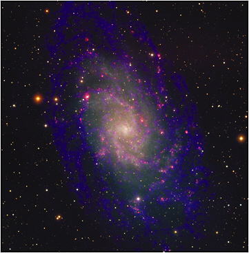
FIGURE 3.3 Combined radio and optical images of M33 (Triangulum Galaxy) by T. Rector, National Radio Astronomy Observatory, and M. Hanna, National Optical Astronomy Observatory. The locations and expected motions of two sites of H2O masers from massive star-forming regions are indicated. Very Long Baseline Array observations over a period of 3 years have yielded the relative motions of these masers; thus one can “see” the Galaxy rotate. Combining this measurement with the rotation speed and inclination (from HI data) of the Galaxy gives a direct measurement of its distance. Courtesy of National Radio Astronomy Observatory/Associated Universities, Inc., and National Optical Astronomy Observatory/Association of Universities for Research in Astronomy/National Science Foundation.
of the 22.235 GHz weak water-vapor absorption line display these characteristics and are widely used as the primary radiometric channel for estimates of integrated precipitable water vapor and path delay.
The atmospheric index of refraction, N, governs the propagation velocity. In the propagation medium (e.g., the atmosphere), the magnitude of N is in turn governed by temperature, pressure, and watervapor density. For a radio wave propagating between the surface and a point outside the atmosphere, the electrical radio wave path length is longer than the physical path length. The difference is called the excess electrical path length. This value is a function of the integrated profile of N along the path. The ability to measure N accurately is important in many applications, including radar altimetry of ocean-surface height (the error for state-of-the-art systems is <2 cm) and radio astronomical observations using very long baseline interferometry. Radar mapping of the height of the ocean surface is critical to the understanding of ocean circulation, including the identification of gyres and stream boundaries that channel significant amounts of heat throughout the ocean.
It is noted that the same bands that are used to measure water vapor from space are also used on ground- and ship-based radiometers to measure integrated precipitable water vapor from the surface of Earth. These ground-based sensors are becoming widely used around the globe to help initialize numerical weather-prediction models and for the calibration of remote sensing satellites. Although they do not provide global measurements, they are particularly accurate over both land and water, since they view water vapor against a strong contrasting background caused by the cold cosmic emission temperature of 2.73 K.
3.5.6
Cloud Liquid Water
For nonprecipitating clouds, microwave radiometric brightness temperatures near 10, 18, and 37 GHz can be used to estimate the integrated amount of cloud liquid water to within ~0.05 mm or 10 percent total columnar water precision. Within the next 5 to 10 years, inclusion of cloud microphysics in climate models is expected. Measurements of cloud liquid water will be needed to diagnose and validate these cloud models, which in principle have the ability to greatly improve understanding of climate, rainfall variability, and the atmospheric radiation budget. The inclusion of cloud water into numerical weather-prediction models will also provide an important means of accurately modeling the influences of short- and long-wave radiation on the evolution of severe weather. Accurate measurements of cloud water amounts also play an important role in global climate models and in understanding the impact of anthropogenic and natural aerosols on clouds, rainfall, and climate.
As with water vapor, the same bands that are used to measure cloud liquid water from space are also used on ground- and ship-based radiometers to measure cloud liquid water from Earth’s surface, but with greater accuracy because of the cold cosmic background. Widespread global deployment of these sensors is occurring.
3.5.7
Soil Moisture
See § 3.3.7 for applications of soil moisture.
3.5.8
Snow Cover
Snow cover and snow water equivalent are derived from microwave radiometric imagery primarily at 18, 23, and 37 GHz, with atmospheric sounding data to remove the atmospherically induced noise in the retrieval. Snow-cover information under clear or cloudy conditions is achievable using microwave
radiometers in LEO at a spatial resolution of ~20 km. Microwave measurements provide important continuity of snow-cover measurements under cloudy conditions when visible and/or IR measurements cannot view Earth’s surface.
Forecasts of river stages, avalanche danger, spring flooding, air rescue conditions, freshwater resources, and soil trafficability all heavily depend on snow-cover information, especially in data-sparse and/or data denied areas where dependence on remotely sensed data is high. Snow-cover and -depth retrievals using microwave radiometric window bands (e.g., 18, 37, and 89 GHz) provide input to numerical land-surface and hydrological forecast models.
Snow cover also plays an important role in the understanding of climate change. For example, continental-scale annual average snow cover, which is easily detectable from satellites (using microwave data to ensure that cloudy conditions do not affect the average), may be a sensitive early indicator of atmospheric warming or cooling. Snow-cover changes also produce strong feedback to the atmospheric energy budget because of the large changes in surface albedo caused by the presence or absence of snow. This feedback is important on both short-term, seasonal-to-interannual, and longer-term (annual to decadal) timescales. Snow-cover measurements over sea ice also provide important information on the flux of heat from the ocean to the atmosphere as modulated by the insulating properties of overlying snow layers.
3.5.9
Sea-Surface Wind Speed and Direction
Sea-surface wind speed is derived very accurately from brightness temperature data collected from LEO at 18 and 23 GHz. Measurements at 37 GHz and near 10 GHz also support these retrievals by helping correct for clouds and water vapor. Wind-speed retrieval accuracy better than 1 m/s uncertainty has been demonstrated with current on-orbit radiometric systems. Further improvements are expected with simultaneously retrieved wind-direction information.
Wind-speed data with <2 m/s uncertainty are needed as inputs to prepare tropical cyclone warnings, initialize numerical weather-prediction models, derive sea state, and for use in ship and aircraft routing, flight safety, and other operations such as data buoy dispersions.
The sea-surface wind vector (both speed and direction) has been retrieved using radar scatterometry on spaceborne and airborne experimental systems operating near 13 GHz (NASA Scatterometer [NSCAT]). Spaceborne scatterometer wind retrieval performance is on the order of ~1 m/s and ± 20° directional uncertainty. Sea-surface wind direction may also be derived using highly sensitive passive polarimetric measurements at 10, 18, 23, and 37 GHz. This technique has been demonstrated with several airborne campaigns and the WindSat spaceborne passive microwave sensor. Sea-surface wind vector can be retrieved using polarimetry at levels of uncertainty similar to those that have been demonstrated with radar scatterometry, but with less saturation in speed at high winds than is possible with scatterometers.
A U.S. Navy study concluded that skill in sea-surface wave forecasting depends heavily on the skill of predicting sea-surface winds. At 20 km horizontal resolution, sea-surface winds from a polar-orbiting weather satellite with a measurement accuracy of ± 2 m/s or ± 10 percent (whichever is greater) will yield open-ocean wave heights within errors of 10 to 20 percent and wave energy within 20 to 50 percent. Such systems provide accurate wind and wave data to support both ocean-based defense operations and commercial shipping. Sea-surface wind-speed and -direction data also support numerical weather-forecasting models of the National Center for Environmental Prediction.
3.5.10
Sea Ice
Measurement of sea-ice characteristics, including ice age, ice type, and ice coverage and motion, is derived from microwave radiometric imagery at 18, 23, and 37 GHz. Ice-surface temperature can be estimated from the microwave imagery; the retrieved values are much less dependent on clouds and atmospheric variability than are measurements obtained from IR brightness temperatures. Sea-ice type is determinable as first-year ice and multiyear ice with a greater than 70 percent confidence level. The state of ice in early formation, such as new ice and young ice, as well as the state of “old” ice (ice age between first year and multiyear) is also detectable, albeit with somewhat less confidence. Ice motion is generally detectable using microwave radiometric imagery to ~1 km per day motion, depending on the atmospheric and surface state.
Arctic and Antarctic operations, maritime commerce, and oceanographic and climate research are extremely dependent on sea-ice-cover, ice-age, and ice-motion data derived from satellite imagery. When sea ice obtains a specific age and/or thickness, icebreaker support is mandatory to prevent vessel damage. Old ice achieves significant tensile strength as it becomes compacted over time and as salinity is lowered. Similarly, submarine surfacing operations are highly dependent on sea-ice concentration and ice-cover thickness. Ridging of old ice can result in ice keels penetrating to tens of meters below the sea surface, posing a significant hazard to submarine navigation. The marginal ice zone (the zone of sea ice between open sea and inner ice pack) is subject to significant variability in response to oceanographic and atmospheric forcing. Vessels that are not ice-strengthened risk damage if sea ice is advected into their operating area due to such forcings.
For climate studies, changes in polar ice cover are primary indicators of global climate change. Reductions in Arctic sea-ice cover are anticipated to significantly affect the global balance of solar heating and atmospheric temperature, moisture, and cloud cover. Changes in polar ice cover will also alter the ecological balance in the Arctic and Antarctic regions.
3.5.11
Sea-Surface Altimetry
Radar altimetry from low-Earth-orbiting platforms is performed using single- and dual-frequency radar altimeters operating at ~13.6 GHz and 5.3 GHz to derive sea-surface height and ocean topology data. Future systems may also utilize 35.5 GHz. The typical precision of these measurements is 3-4 cm over a range of ~200 meters and 4-5 cm overall after orbital variations are accounted for. To achieve this accuracy, precise estimates of the excess path delay derived from radiometric measurements near 22.235 GHz are also required. (See § 3.5.6.)
For operational oceanography and forecasting, sea-surface height/topography observations from polar-orbiting weather satellites provide the only means of acquiring the high-quality global data needed to analyze transient ocean current features (i.e., eddies) to the resolution and accuracy required for emerging coupled ocean-atmospheric models.
For climate monitoring and assessment, sea-surface altimetry and sea-level data are applicable to many areas of study. In the tropical oceans, sea level provides estimates of the upper-level heat content, which is important for numerical ocean-forecast models. State-of-the-art altimeters are sufficient to determine the general circulation and its variability accurately enough to allow a quantitative assessment of the ocean’s role in Earth’s climate, hydrological, and biochemical systems. In addition, ocean altimetry systems allow the observation of changes to shorefast continental ice.
3.5.12
Ice-Surface Temperature
The temperature of the ice surfaces on either land or water to ~1 K measurement uncertainty is required from the next-generation operational microwave radiometers operating in LEO. The data may be derived using radiometric brightness temperatures at 10, 18, 23, and 37 GHz, with additional support with atmospheric characterization from sounding in the 50-56 GHz and 183 GHz spectral regions.
Surface temperatures are not available in data-sparse regions throughout the Arctic and Antarctic, making estimations of ice thickness difficult and potentially inaccurate. Remotely sensed ice-surface temperature maps produced on a daily basis will be invaluable for estimating sea-ice growth and decay. The temperature uncertainty must be accurate to within 1°C to ensure an accurate calculation of frost degree-day information.
3.5.13
Microwave Radiometric Imagery
Many meteorological and surface environmental data products are produced using multivariable algorithms to retrieve a set of geophysical parameters simultaneously from calibrated multichannel microwave radiometric imagery. For example, sea-surface temperature, wind speed, water vapor, and cloud water are simultaneously estimated using multichannel imagery from NASA’s Tropical Rainfall Measurement Mission (TRMM) Microwave Imager. If one or more bands were removed from the imagery set, the ability to perform the multivariable estimate would be inhibited. In general, radiometric measurements over the range from ~6 to >183 GHz using EESS-allocated frequencies—and in some cases additional bands not allocated to the EESS—are used for the generation of microwave-based imagery. In addition to the lists in the tables in this handbook, a list of useful microwave bands and radiometric imagery products can be found in ITU-R SA.515.
3.5.14
Sea-Surface Temperature
Sea-surface temperature is measured using passive microwave channels at 10.7 GHz. While not as sensitive as those measurements at 6.8 GHz, the higher frequency provides finer spatial resolution for the same-size antenna aperture. For applications of SST, see §.4.4.
3.6
BANDS BETWEEN 25 AND 50 GHZ
The frequency region between 30 and 40 GHz is the first atmospheric window in the millimeter radio region where ground-based observations can be made. On either side of this frequency band, water and oxygen molecules in Earth’s atmosphere attenuate the incoming radiation. The O2 absorption beginning at ~50 GHz is sufficiently strong to render ground-based observations impossible. Conversely, the contrast between an opaque atmosphere at the edges of this band and a transparent atmosphere within the band provides the means for measuring various terrestrial parameters (see Table 3.5).
3.6.1
Atmospheric Effects on Earth-Surface Parameter Retrieval
Algorithms performing retrieval of Earth-surface parameters using passive microwave radiometry often use simultaneous measurements of emissions at 18 and 23 GHz. In general, thermal emissions originating from Earth’s surface over this frequency range exhibit few or readily predictable variations
TABLE 3.5 Frequency Allocations Between 25 and 50 GHz: Bands, Services, Footnotes, and Scientific Uses
|
Band (GHz) |
Services |
Footnotes |
Scientific Use |
|
25.5-27 |
EESS (S→ E), FS, ISS, MS, sftss (E→ S) |
|
|
|
27-27.5 |
5.536, 5.5376 |
|
|
|
28.5-29.5 |
FS, FSS (E→ S), MS, eess (E→ S) |
5.5417 |
|
|
29.5-30 |
5.541, 5.54210 |
|
|
|
31.0-31.3 |
FS, MS, sftss (S→ E), srs, (ras) |
Atmospheric water vapor, precipitation |
|
|
31.3-31.5 |
EESS (passive), RAS, SRS (passive) |
Continuum, complex organic molecules |
|
|
31.5-31.8 |
EESS (passive), RAS, SRS (passive), fs,17 ms18 (excluding aems) |
Cloud water, precipitation |
|
|
31.8-32 |
FS,21 RNS, SRS (deep S→ E) |
DSN downlinks |
|
|
32-32.3 |
FS,26 ISS, RNS, SRS (deep S→ E) |
5.547C,27 5.548, US69, US262 |
DSN downlinks |
|
34.2-34.7 |
RLS, SRS (E→ deep S) |
5.54928 |
|
|
34.7-35.2 |
RLS, srs29 |
5.549 |
|
|
35.5-36 |
MetAids, EESS (active), RLS, SRS (active) |
|
|
|
36-37 |
EESS (passive), FS, MS, SRS (passive) |
Cloud water, precipitation, complex organic molecules |
|
|
37-37.5 |
FS, MS, SRS (S→ E) |
|
|
|
37.5-38 |
FS, FSS (S→ E), MS, SRS (S→ E), eess36 (S→ E) |
|
|
|
38-39.5 |
FS, FSS (S→ E), MS (S→ E), eess37 |
|
|
|
39.5-40 |
FS, FSS (S→ E), MS, MSS, eess38 (S→ E) |
|
|
|
40-40.5 |
EESS (E→ S), eess (S→ E), FS,39 FSS (S→ E), MS, MSS (S→ E), SRS (E→ S) |
|
|
|
42.5-43.5 |
FS, FSS (E→ S), MS (excluding AeMS), RAS |
Continuum, VLBI, SiO masers |
|
|
48.94-49.04 |
RAS, FS, FSS, MS |
CS |
|
|
NOTE: For definitions of acronyms and abbreviations, see Appendix I. For information about other features of this table, see §3.1.2, “Note to the Reader Regarding Frequency Allocation Tables.” 15.536 limits ISS to SRS, EESS, and IMS applications. 25.536A: EESS Earth stations cannot claim protection from FS and MS stations in neighboring countries. |
|||
across this range. Atmospheric attenuation under clear conditions is a function of water vapor and cloud amount for the 18 and 37 GHz bands, with measurements near 22.235 GHz showing higher attenuation than those of either window region owing to water vapor. Therefore, under clear conditions, algorithms benefit from noise reduction due to multiple independent measurements of the surface emission. Also, because the ~22.235 GHz measurements exhibit an additional dependence on integrated water vapor, the effects of atmospheric water vapor can be corrected in part, resulting in less residual systematic error due to the atmosphere.
An additional value of measurements in the region of ~37 GHz and/or ~31 GHz is the factor of ~2 improvement in horizontal spatial resolution (HSR) from diffraction-limited antennas compared with the HSR available at 18 GHz. The HSR requirements are often a key attribute for the retrieval of surface parameters, particularly over land, where data utility improves, in principle, for retrievals of homogenous pixels. However, under increasingly cloudy conditions, extinction due to Mie scattering and absorption more rapidly affects 37 GHz measurements, lowering their sensitivity to surface emission. Therefore, in principle, a mechanism exists for estimating cloud amounts and/or for removing some of the effect of clouds, preventing biasing of surface-parameter retrievals.
Many retrievals of surface and atmospheric environmental parameters in microwave remote sensing are carried out using a core combination of ~18, ~23, and ~37 GHz emission measurements. A partial list of these environmental parameters includes precipitation (§3.5.2), precipitable water (§3.5.5), cloud liquid water (§3.5.6), soil moisture (§3.5.7), snow cover (§3.5.8), sea-surface winds (§3.5.9), sea ice (§3.5.10), and ice surface temperature (§3.5.12). If atmospheric temperature and/or moisture sounding channels are available, they can also be included to provide additional aid in removing the effects of atmospheric variability.
3.6.2
SiO Masers
The 42.5-43.5 GHz band contains the lowest rotational transitions (J = 1 → 0) of vibrational states of SiO. These transitions have been detected as strong maser emission from the envelopes of evolved stars and in young star-forming regions. VLBI measurements of these masers are providing probes of instellar envelopes, yielding information on temperature, density, stellar wind velocities, and envelope geometry.
3.6.3
Carbon Monosulphide
The 48.94-49.04 GHz band contains the lowest rotational transitions of CS and its isotopes such as C33S and C34S. They serve primarily as a tracer of dense cold molecular clouds. Since CS is a relatively high density tracer, whereas CO is a low-density tracer, this species can also be an important diagnostic of the molecular material in other galaxies, and in particular the active nuclei and starburst galaxies.
3.6.4
Organic Acetylenic Chains
The spectral region from 30 to 50 GHz contains the strongest lines of HC3 N, a molecule that is a signpost of pre-protostellar conditions and a good temperature probe for extremely cold gas. It represents the shortest of a series of long-chain molecules of the form HCxN (x = 1, 3, 5, 7, 9, 11, …).
3.6.5
Continuum and Very Long Baseline Interferometry
The region is important for defining the high-frequency continuum spectra of galactic and extragalactic objects. For example, at these frequencies, one can observe emission from dust in extremely dense cores, which are opaque at higher frequencies.
3.6.6
Microwave Radiometric Imagery
See §3.5.13 for applications of microwave radiometric imagery.
3.7
BANDS BETWEEN 50 AND 71 GHZ
The bands, services, footnotes, and scientific observations for each band in the allocations between 50 GHz and 71 GHz are presented in Table 3.6.
3.7.1
Atmospheric Temperature Profiling
Retrieval of the atmospheric temperature profile using passive sounding in the ~50-62 GHz region uses the multitude of spin-rotational O2 transitions in this region. Atmospheric attenuation varies from ~1 dB near ~50 GHz for clear atmospheric conditions to >200 dB at nadir for selected frequencies within ~58 to ~62 GHz. This characteristic provides the ability to estimate the atmospheric temperature within a specific altitude region by a careful selection and control of channel frequency. Atmospheric temperature profiles can be measured with an uncertainty of ~1 K with ~1-1.5 km altitude resolution to support a large variety of operational and scientific applications. The same oxygen resonance frequency that enables these measurements also leads to the strong absorption of terrestrial anthropogenic emissions, so that in many (albeit not all) cases the spectrum from ~58 to ~62 GHz can be shared with terrestrial active systems without interference.
Atmospheric profiles of temperature from polar-orbiting satellites are required to initialize the current and emerging global ocean-atmosphere models. These models provide essential global meteorological and oceanographic predictions for many civil and military applications. High profile-measurement accuracies are essential for proper operation and input for prediction models. For example, it has been shown that for temperature profile inputs not meeting 1 K to 3 K (depending on altitude) uncertainty, the profile data corrupt the model rather than increase its capability to forecast. Observational errors, usually on smaller scales, amplify the model error and, through nonlinear interactions, gradually spread to longer scales, eventually destroying forecast skill. In previous studies, numerical models using data with a standard deviation of 0.5°C at all levels had an exponential error growth with a doubling time of about 2.5 days. Similar results were found for other data types (i.e., winds, moisture, and so on), with forecast errors as high as 20 to 30 percent.
Atmospheric circulation is the main driver of regional changes in near-surface wind, temperature, precipitation, soil moisture, and other surface variables. These variables constrain the ability to make use of Earth’s resources and sustain humanity’s existence. Variations in these variables are strongly related through large-scale features of the atmospheric circulation as well as through interactions involving land and ocean surfaces. Atmospheric circulation is in turn dependent on the variables that define its structure and on dynamics such as wind speed and direction, temperature, humidity, and geopotential height. Two well-known examples of large-scale features are the El Niño-Southern Oscillation and the North Atlantic Oscillation, both of which are a product of global-scale climate fluctuations. Evidence from satellites globally observing associated changes in atmospheric variables may enhance the understanding of the specific relationships between surface and atmospheric variables and provide a better basis for validation of those relationships.
Currently, atmospheric temperature profiles are measured using LEO satellite microwave sounders. A number of present-day technological developments are enabling the future deployment of a geostationary orbiting microwave temperature sounder.
3.7.2
Mesospheric Temperature Profile
Within the ~50 to 62 GHz O2 complex, spectrum near the strongest oxygen transitions (e.g., 9+ and 7+) is used to measure temperature profiles in the upper atmosphere from ~40 to ~90 km in altitude. The
TABLE 3.6 Frequency Allocations Between 50 and 71 GHz: Bands, Services, Footnotes, and Scientific Uses
|
Band (GHz) |
Services |
Footnotes |
Scientific Use |
|
50.2-50.4 |
Temperature profiling |
||
|
51.4-52.6 |
5.55611 |
|
|
|
1-3 52.6-54.25 |
EESS (passive), SRS (passive) |
5.340, 5.556, US24612 |
Temperature profiling, interstellar O2 |
|
54.25-55.78 |
EESS (passive), ISS, SRS (passive) |
|
|
|
54.25-56.9 |
EESS (passive), FS, ISS, MS, SRS (passive) |
|
|
|
56.9-57 |
EESS (passive), FS, ISS, MS, SRS (passive) |
5.557, US26320 |
|
|
57-58.2 |
EESS (passive), FS, ISS, MS, SRS (passive) |
5.556A, 557, US26321 |
|
|
58.2-59 |
5.547, 5.556, US246 |
Interstellar O2 |
|
|
59.0-59.3 |
EESS (passive), FS, ISS, MS, RLS, SRS (passive) |
5.556A, 5.558, 5.559, US353 |
|
|
NOTE: For definitions of acronyms and abbreviations, see Appendix I. For information about other features of this table, see §3.1.2, “Note to the Reader Regarding Frequency Allocation Tables.” 1In the United States only. 2In the United States only. 35.340 prohibits all emissions. 45.555A allowed FS and MS as primary until July 1, 2000. 5US263 cancels protection of EESS and SRS from FS and MS. 6Except in the United States. 7Except in the United States. 8Only in the United States. 9Only in the United States. 10Only in the United States. 115.556 notes that radio astronomy observations may be carried out under national arrangements. 12US246 forbids all emissions. 135.556B adds MS on a low-density basis in Japan. 14Old series international footnote 909 allows AeMS subject to not causing harmful interference to ISS. 15US263 cancels protection of EESS and SRS from FS and MS. 165.556A limits use of this band by ISS. 175.557 adds RLS on a primary basis in Japan. 185.558 allows AeMS subject to not causing interference to ISS. 19US263 cancels protection of EESS and SRS from FS and MS. 20US263 cancels protection of EESS and SRS from FS and MS. 21US263 cancels protection of EESS and SRS from FS and MS. 22Except in the United States. 23Except in the United States. 24In the United States only. |
|||
Defense Meteorological Satellite Program Special Sensor Microwave Imager Sounder will use frequencies between ~60.4 and 61.2 GHz and a separate channel near 63 GHz to obtain such mesospheric temperature profiles. Splitting of the strong O2 transitions by Earth’s magnetic field provides vertical response (or, weighting) functions that depend on the polarization of the received signal.
3.8
BANDS BETWEEN 71 AND 126 GHZ
In addition to the bands listed in Table 3.7, the 78.00-79.00 GHz EESS active band is to be used for cloud monitoring and should be specifically listed rather than being relegated to a footnote, since it is a primary allocation. The spectrum within 102 and 126 GHz is not entirely allocated to EESS passive, but rather is broken into 102-105 GHz, 105-109.5 GHz, 109.5-111.8 GHz, 114.25-116 GHz, 116-119.98 GHz, and 119.98-122.25 GHz segments with different sharing services. EESS passive service is allocated only in the 109.5-111.8 GHz and 114.25-122.25 GHz bands. Per NTIA’s Redbook, even the Radio Astronomy Service allocation is fragmented: primary between 76 and 77.5 GHz, secondary from 77.5 to 78 GHz, primary between 78 and 116 GHz. The fragmentation of the 71-106 GHz spectral region is unfortunate and should be addressed at future World Radiocommunication Conferences.
3.8.1
Interstellar Molecular Lines
Since there is relatively little absorption from atmospheric O2 and H2O, the 3 mm band between 65 and 115 GHz is perhaps one of the best high-frequency regions for both continuum and line observations of celestial objects. In particular, this band contains the fundamental (J = 1 → 0), or lowest-energy, transition of most common interstellar molecules, including CO, HCO+, HCN, CCH, CN, HNC, HCO, HNO, H2CO, and N2H+. More than 100 molecules have been detected in this frequency range, as have 25 different isotopic species. These also include favorable transitions of such simple molecules as SO, SO2, SiO, SiS, and MgNC and such complex molecules as CH3CH2OH, CH3CH2CN, and CH3OCH3. Two vibrational states of the transitions of SiO fall in this range; SiO is one of the few molecules
TABLE 3.7 Frequency Allocations Between 71 and 126 GHz: Bands, Services, Footnotes, and Scientific Uses
|
Band (GHz) |
Services |
Footnotes |
Scientific Use |
|
72.77-72.91 |
FS, FSS (E→ S), MS, MSS (E→ S), RAS1 |
HC3N (important lines at 72.039 GHz for DCO+ and 72.415 GHz for DCN) |
|
|
74-75.5 |
FS, FSS (S→ E), MS, srs5 (S→ E) |
US2976 |
HCNH+, N2 O, H2 CO |
|
75.5-76 |
AeMS, AeMSS, srs7 (S→ E) |
|
|
|
76-81 |
RAS (except secondary between 77.5-78), RLS, aems,8 aemss,9,10 srs11 (S→ E) |
5.56012 |
HDO |
|
81-84 |
RAS, FS, FSS (S→ E), MS, MSS (S→ E), srs13 (S→ E) |
|
C3H 2, HC3N |
|
84-86 |
RAS, FS, MS, BS, BSS, (ras) |
US21114 |
NH2 D, CH3CCH |
|
86-92 |
EESS (passive), RAS, SRS (passive) |
SiO, H13CO+, HCO+, HCN, CCH, HNC, CH3CN, HC15N, H 13CN, HN13C, HCO |
|
Band (GHz) |
Services |
Footnotes |
Scientific Use |
|
92-94 |
FS, FSS (S→ E), MS, RLS, RAS |
5.149, 5.556 |
13CS, N2H+ , AlNC |
|
94-94.1 |
EESS (active), RLS, SRS (active), RAS |
5.56218 |
Cloud radar |
|
95-100 |
MS, MSS, RNS, RNSS, RAS19 |
5.149, 5.55520 |
CS, SO, C34S, MgNC |
|
100-102 |
5.341,23 US246 |
Extragalactic CO, HC3N |
|
|
102-105 |
5.341, US211 |
CH3CCH |
|
|
105-116 |
EESS (passive), RAS, SRS (passive) |
5.340, 5.341, US74, US246 |
SO, CN, CO, 13CO, C18O, C17O, 13CN |
|
116-119.98 |
EESS (passive), FS, ISS, MS, SRS (passive) |
5.341, 5.558, US211, US263 |
|
|
119.98-120.02 |
EESS (passive), FS, ISS, MS, SRS (passive), aems |
5.341, US211, US263 |
|
|
120.02-126 |
EESS (passive), FS, ISS, MS, SRS (passive) |
Temperature profiling |
|
|
NOTE: For definitions of acronyms and abbreviations, see Appendix I. For information about other features of this table, see §3.1.2, “Note to the Reader Regarding Frequency Allocation Tables.” 1In the United States only. 25.149 urges protection of RAS in this band. 35.556 allows RAS under national arrangements. 4US270 adds RAS to this band within the larger 71-74 GHz band. 5Except in the United States. 6US297 allows feeder links for BS. 7Except in the United States. 8Primary in the United States between 77.5 and 78 GHz. 9Primary in the United States between 77.5 and 78 GHz. 10In the United States only above 77 GHz. 11Primary in the United States between 77.5 and 78 GHz. 125.560 allows radars on space stations to be operated between 78 and 79 GHz on a primary basis for EESS and SRS. 13Except in the United States. 14US211 urges additional protection to RAS from adjacent bands. 155.340 prohibits all emissions. 16US74 limits protection of RAS from extraband radiation. 17US246 prohibits all emissions. 185.562 limits EESS and SRS to spaceborne cloud radars. 195.555 adds RAS as primary between 97.88 and 98.08 GHz. 205.555 adds RAS as primary between 97.88 and 98.08 GHz. 21Except in the United States. 22Except in the United States. 235.341 draws attention to SETI research in this band. 24Except in the United States. 25In the United States. 265.138 allows ISM applications subject to special agreements. 27US263 specifies that EESS and SRS will not be protected from FS and MS. |
|||
showing maser emission and the only one showing strong maser emission in an excited vibrational state. N2H+, HCS+, HCNH+, and HCO+ are vitally necessary participants in the ion-molecule reactions believed to be key in the formation of many other molecules in the interstellar gas. Furthermore, some molecules have several isotopic species in this range, so that isotopic abundance ratios can be studied. As an example, the basic molecule HCN has the isotopic species H12C14N, H3C14N, and H12C15N in the 86-92 GHz range, and all have been observed in the interstellar gas. It is clear that this region of the millimeter spectrum will remain one of the most-used for radio astronomy.
3.8.2
Carbon Monoxide
The discovery of interstellar CO at 115.271 GHz has been of fundamental significance for the subject of astrochemistry. This is primarily because CO is a relatively stable molecule compared with other molecules discovered in the interstellar medium, and also because CO seems to be very abundant and exists almost everywhere in the plane of our Galaxy as well as in a number of other galaxies. Studies have yielded new information on the distribution of gas in spiral galaxies. Allowance for Doppler shifts characteristic of nearby and even distant galaxies is essential for adequate protection of radio spectral lines.
Because the CO molecule is so ubiquitous and therefore present under nearly all physical and chemical conditions, its emission is the principal tool available to astronomers today for the study of the star-forming gas in the Milky Way Galaxy, and even in quite distant galaxies. CO studies give information about disks around forming stars and, in the future, with the expansion of millimeter-wave interferometer instruments, they may tell of the conditions for planet formation. Furthermore, CO emission studies reveal the presence of bursts of star formation activity in nearby and, in some cases, distant galaxies. These bursts have recently been related to collisions between galaxies and possibly to the formation of massive black holes and quasars. CO lines are also used to measure the mass loss rates from late-type stars.
The 100-102 GHz band is used for radio astronomy observations of redshifted CO in distant galaxies.
The 200-300 GHz band contains the second available rotational line of carbon monoxide (12C16O), together with its isotopic variants 13C16O and 12C18O. These are very strong and important lines both within our Galaxy and in distant galaxies. In combination with the first lines in the 106-116 GHz band, they permit the determination of the physical characteristics of the gas within the galaxies. The coverage for 12C16O extends to galaxies at velocities of 2000 km/s, but it should be much greater in order to give protection to the work of learning about the structure and evolution of much more distant galaxies in the future.
3.8.3
Isotope Ratios
One important use of molecular lines is the study of isotope ratios, in particular, the 12C/13C, 16O/ 18O, and 32S/34S ratios. These ratios give important insight into theories of nucleosynthesis in stars and models of star-formation rates and the relative masses involved, that is, galactic chemical evolution. The important molecules in this context are 12CO, 13CO, and 18CO; 12CN and 13CN; and 12CS, 13CS, and C34S. The fundamental transitions of CO and CN and their isotopomers are in the 3 mm band, as well as favorable lines of CS. All of these species are important isotopic tracers.
Molecules can also be used to investigate deuterium/hydrogen ratios. Because of chemical fractionation, very high deuterium/hydrogen ratios are found in certain interstellar molecules as a result of ion-
molecule chemistry. DCN and DCO+ are important tracers in this context. Their lowest-energy spectral transitions lie near 72 GHz.
3.8.4
Interstellar and Circumstellar Chemistry
The 3 mm band, along with the 2 mm window, is particularly relevant to studies of interstellar chemistry, as these bands contain favorable transitions of most known molecules. As mentioned, species of interest include molecular ions such as HCO+ and HCNH+, the free radicals CN and CCH, and a large number of organic molecules, including C3H2, CH3OH, CH3CH2CN, CH3COCH3, and CH3OCHO. Also, the spectral lines originating from long-chain carbon species such as C3H, C3N, C4H, C7H, C8H, and so on are prominent in these bands, as well as those of silicon-, magnesium-, and aluminum-bearing molecules (SiS, SiC2, SiC3, MgCN, AlCl, AlNC, and so on). The long-chain molecules and the refractory species play significant roles in the chemistry of circumstellar envelopes of late-type stars.
3.8.5
Astrobiology
Some theories posit that interstellar chemistry may have supplied the prebiotic compounds essential for terrestrial life. Consequently, establishing the inventory of organic molecules in interstellar gas is of interest to the study of the origin of life. Because organic molecules have many favorable transitions at millimeter wavelengths, this spectral region is crucial for the identification of such species. The 2 and 3 mm spectral regions have been the prime wavelength regions for the detection of organic molecules. Many possible new organic compounds may be identified in interstellar gas. It is important to recognize that new frequencies are regularly becoming available for possible new molecules, and hence broadband protection of the 2 and 3 mm windows is desirable.
3.8.6
Atmospheric Temperature Profile
The atmospheric temperature profile can be derived using passive radiometric measurements on and near the 118.75 GHz O2 transition. Temperature profiles derived from this band complement those derived using the 50-60 GHz complex by providing independent measurements, albeit with reduced sensitivity at higher altitudes and less penetrability of clouds and precipitation. However, diffraction-limited apertures of fixed size will yield temperature profiles with better horizontal spatial resolution with 118 GHz measurements compared with data from 50-60 GHz. As a result, channels near 118 GHz are being considered for use in sonding and imaging from a geostationary microwave sensor. Moreover, the difference in response between similar clear-air channels at 50-60 GHz and ~118 GHz will provide additional information on cloud and precipitation amounts.
3.8.7
Precipitation
Passive microwave measurements near 89 GHz play an important role in the retrieval of precipitation data, particularly over land. Owing to the combination of high emissivity and cloud thickness and temperature over land, signatures of convective precipitation cells are often strongest at 89 GHz. At this frequency there is high sensitivity to clouds over land, causing the upwelling brightness temperatures to be cooler rather than warmer, as observed over a relatively cold ocean background. Clouds over land exhibit much less contrast at lower microwave window frequencies (e.g., 10, 18, and 37 GHz) causing 8 GHz observations to play an important role in determining rain rate over land. See also §3.5.2.
3.8.8
Cloud Base Height and Cloud Parameters
A spaceborne 94 GHz cloud-profiling radar (CloudSat) was successfully launched in May 2006, with an objective of measuring the altitude and properties of clouds with 500 m vertical resolution, 1.2 km cross-track resolution, and with a sensitivity of −30 to −36 dBZ (decibels of Z, where Z is the energy reflected back to the radar, or reflectivity). This advanced W-band radar will gather information on the vertical structure of highly dynamic cloud systems to provide global measurements of cloud properties. These measurements will help scientists compile a database of cloud properties to improve the representation of clouds in global climate and numerical weather-prediction models.
Cloud base information for a range of cloud types, particle distributions (microphysics), and liquid water content is desired to support both operational and scientific objectives. Ceiling height data are vital to identify regions of potential aircraft icing and for determining the most effective altitudes for commercial flight operations. For climate measurements, cloud base height is critical for determining the long-wave energy budget at Earth’s surface, and for understanding the impacts of anthropogenic aerosols on cloud formation, precipitation, and short- and long-wave energy fluxes.
3.8.9
Microwave Radiometric Imagery
See §3.5.13 for applications of microwave radiometric imagery.
3.9
BANDS BETWEEN 126 AND 400 GHZ
In addition to the bands listed in Table 3.8, the 130-134 GHz and 237.9-238 GHz (cloud radars only) are EESS active bands. The 155.5-158.5 GHz EESS passive band expires January 1, 2018.
3.9.1
Molecular Lines
The atmospheric windows at 1 mm (200-300 GHz) and 0.8 mm (325-375 GHz) contain a wide range of interstellar molecules. The J = 3 → 2 and J = 4 → 3 transitions of such species as HCO+ and HCN are important tracers of high-density gas in the molecular clouds. The J = 2 → 1 and J = 3 → 2 lines of CO, as well as its isotopic variants, lie in these bands. Multiple transition studies of CO enable the density and temperature profiles of molecular clouds to be determined and are used as tracers of the total amount of molecular gas. Also in these wavelength regions, diatomic hydride and polyatomic hydride species have some of their lowest-energy rotational transitions, such as MgH, KH, H2O, and H3O+. In fact, only at frequencies above 200 GHz can these hydride molecules be studied in the interstellar medium. Because they contain hydrogen atoms bonded to one heavier atom, they rotate very quickly. Therefore, their rotational transitions lie at higher frequencies than those of other interstellar molecules. Investigating simple hydride species is crucial for interstellar chemistry. Because of the high abundance of hydrogen, such species are prevalent in molecular clouds and are the initial species produced by interstellar chemistry.
Passive measurements near the 183.31 GHz water-vapor line, aided by measurements in the adjacent transmission window at the EESS-allocated bands of 150-151 GHz or 164-168 GHz, are critical for the global measurement of atmospheric water-vapor profiles. Measurements from spaceborne sensors in LEO are carried out to obtain atmospheric water-vapor profiles from Earth’s surface to 100 mb with a measurement uncertainty of ~20 percent and ~35 percent for clear and cloudy conditions, respectively. These measurements are used to support meteorological forecasting and climatological modeling. Mois-
TABLE 3.8 Frequency Allocations Between 126 and 400 GHz: Bands, Services, Footnotes, and Scientific Uses
|
Band (GHz) |
Services |
Footnotes |
Scientific Use |
|
140.69-140.98 |
MS, MSS, RAS, RNS,RNS, rls |
H2 CO |
|
|
144.68-147.12 |
RLS, aems, aemss, RAS4 |
5.149, 5.555 |
H2CO, DCN (Note: DCO+ at 144.07 GHz) |
|
148.5-151.0 |
EESS (passive), RAS, SRS (passive) |
US246 |
|
|
150-151 |
EESS (passive), FS, FSS (S→ E), MS, SRS (passive), ras |
NO, H2 CO |
|
|
151-156 |
FS, FSS (S→ E), MS |
US2117 |
CS, CH3CN, CH3CCH |
|
156-158 |
EESS8 (passive), FS, FSS (S→ E), MS |
|
|
|
158-164 |
FS, FSS (S→ E), MS |
US211 |
|
|
164-167 |
EESS (passive), RAS, SRS (passive) |
US246 |
(H2S at 168.7 GHz) |
|
170-174.5 |
FS, ISS, MS, ras9 |
5.149, 5.385 |
|
|
174.8-182.0 |
EESS (passive), FS, ISS, MS, SRS (passive), ras10 |
5.149, 5.385, US263 |
|
|
176.5-182 |
FS, ISS, MS, ras11 |
5.149, 5.385, US211 |
|
|
182-185 |
EESS (passive), RAS, SRS (passive) |
|
|
|
185-190 |
FS, ISS, MS, EESS (passive), ras15 |
5.149, 5.385, US211 |
|
|
190.0-191.8 |
EESS (passive), SRS (passive) |
5.340, US246 |
|
|
200-209 |
EESS (passive), RAS, SRS (passive) |
5.341,16 5.563A, US74, US246 |
|
|
209-217 |
FS, FSS (E→ S), MS, RAS |
5.341, 5.342 |
|
|
217-226 |
FS, FSS (E→ S), MS, RAS, SRS (passive) |
5.562B, 5.341, 5.342 |
|
|
226-231.5 |
EESS (passive), RAS, SRS (passive) |
US246 |
|
|
231.5-235 |
FS, FSS (S→ E), MS, rls |
US211 |
12CO |
|
235-238 |
EESS (passive), FS, FSS (S→ E), MS, SRS (passive) |
US263 |
|
|
250-252 |
EESS (passive), SRS (passive), RAS17 |
5.149, 5.55518 |
NO |
|
261-265 |
MS, MSS, RAS,19 RNS, RNSS |
HCN, CCH |
|
|
265-275 |
FS, FSS, MS, RAS |
5.149 |
HCO+ |
|
275-300 |
5.56524 |
N2H+ |
|
Band (GHz) |
Services |
Footnotes |
Scientific Use |
|
300-400 |
(ras), (eess), (srs) |
5.565 |
CO, CS, CN, HCO+, HCN, MgH, H3O+, SiO |
|
NOTE: For definitions of acronyms and abbreviations, see Appendix I. For information about other features of this table, see §3.1.2, “Note to the Reader Regarding Frequency Allocation Tables.” 15.149 urges protection of RAS. 25.340 forbids emissions from airborne stations and from space stations toward Earth between 140.69 and 140.98 GHz. 35.555 adds RAS as primary in the bands 140.69-140.98 GHz, 144.68-144.98 GHz, 145.45-145.75 GHz, and 146.82-147.12 GHz. 45.555 adds RAS as primary in the bands 140.69-140.98 GHz, 144.68-144.98 GHz, 145.45-145.75 GHz, and 146.82-147.12 GHz. 55.385 adds RAS as secondary in the bands 150-151 GHz, 174.42-175.02 GHz, 177-177.4 GHz, 178.2-178.6 GHz, 181-181.46 GHz, 186.2-186.6 GHz, and 257.5-258 GHz. 6US263 specifies that EESS and SRS will not be protected from FS and MS. 7US211 urges additional protection to RAS from adjacent bands. 8Except in the United States. 9In the sub-band 174.42-175.02 GHz. 10In the sub-band 174.42-175.02 GHz. 11In the sub-bands 177-177.4 GHz, 178.2-178.6 GHz, and 181-181.46 GHz. 125.340 forbids all emissions, but see 5.563. 135.563 adds FS and MS in the United Kingdom. 14US246 forbids all emissions. 15In the sub-band 186.12-186.6 GHz. 165.341 makes note of SETI observations in this band. 17In the sub-band 250-251 GHz. 185.555 adds RAS as primary for 250-251 GHz and 262.24-262.76 GHz. 19In the sub-band 262.24-262.76 GHz. 205.385 adds RAS as secondary for 257.5-258 GHz. 215.564 makes RAS primary within the larger band 252-265 GHz in Germany, Argentina, Spain, Finland, France, India, Italy, and The Netherlands. 22In the United States. 23In the United States. 245.565 urges that administrations take all practicable steps to protect the passive services from harmful interference in certain designated bands, and other bands yet to be identified, until the next competent World Radiocommunication Conference. |
|||
ture profiles can also be used to support path delay and attenuation estimates for active remote sensing systems (e.g., radar altimetry) and satellite radio-frequency links. Accurate measurements of upper tropospheric water vapor are also obtained by viewing Earth’s limb from LEO to support scientific studies of the upper atmosphere and atmospheric chemistry. In general, measurements near 183 GHz are widely used. Observation from geostationary orbit is planned in the future.
3.9.2
Atmospheric Water-Vapor Profile
The hydrologic cycle is critical to the dynamical and thermodynamical functioning of the global climate system and to its impacts on human society. The distributions of water vapor, cloud liquid water, and cloud ice in the atmosphere and the evolution of these distributions with time determine to a great extent the radiation characteristics of clouds, with consequent large impacts on the radiation balance of the atmosphere. Water vapor is an important greenhouse gas, greatly influencing the surface radiation budget even in the absence of clouds. Condensation and evaporation of water in the atmosphere affect large transfers of energy and have enormous influence on large-scale circulation in the troposphere.
Atmospheric profiles of moisture measured from polar-orbiting LEO satellites are required to initialize high-resolution global ocean-atmosphere models that provide the global meteorological and oceanographic predictions necessary for civil and military operations. Much of the atmospheric moisture is concentrated close to Earth’s surface in the lowest ~1.5-2.5 km of the atmosphere. Comparisons of model simulations indicate that if the measurement accuracies of moisture profiles are less than threshold values (generally those values listed above), the remotely sensed profile data that are used as input corrupt the model rather than increases its capability to forecast. Observational errors, usually on the smaller scales, amplify and, through nonlinear interactions, gradually spread to the longer scales, eventually destroying forecast skill. In previous studies, numerical models using data with a standard deviation of 0.5°C at all levels exhibited an exponential error growth with a doubling time of about 2.5 days. Similar results were found for other data types (i.e., winds, moisture, and so on) with forecast errors as high as 20 to 30 percent.
Passive measurements near the strong 183.31 GHz water-vapor line, aided by measurements in the adjacent transmission window at the EESS-allocated bands of 150-151 GHz or 164-168 GHz, are critical for the global measurement of atmospheric water vapor profiles. Measurements from spaceborne sensors in LEO are carried out to obtain atmospheric water-vapor profiles from Earth’s surface to 100 mb with a measurement uncertainty of ~20 percent and ~35 percent for clear and cloudy conditions, respectively. These measurements are used to support meteorological forecasting and climatological modeling. Moisture profiles can also be used to support path delay and attenuation estimates for active remote sensing systems (e.g., radar altimeters) and satellite radio-frequency links. Accurate measurements of upper tropospheric water vapor are also obtained by viewing Earth’s limb from LEO to support scientific studies of the upper atmosphere and associated atmospheric chemistry. In general, water-vapor measurements near 183 GHz are widely used.
3.9.3
Precipitation
Passive microwave remote sensing from satellites and aircraft at frequencies above 90 GHz are used to estimate hydrometeor properties of cirrus clouds and the higher altitude (frozen particle regimes) of convective and anvil clouds. Specific frequencies in use on various systems include 150 GHz, 166 GHz, 183.31± 1 GHz, 183.31± 3 GHz, 183.31±7 GHz, 183.31±10 GHz, 220 GHz, 325 GHz, 340 GHz, 380 GHz, 424 GHz, ~500 GHz, and 640 GHz. These channels are particularly sensitive to the frozen particles, and several have been used to estimate snowfall rate over land surfaces. Furthermore, since these channels tend to become opaque to the land surface in the presence of clouds, they may be useful in estimating light rain over land surfaces. Precipitation observation may be possible with high spatial resolution using a geostationary microwave sounder and frequencies at ~183, 340, 380, and 424 GHz.
It is important to have knowledge of cirrus clouds and the frozen particles in convective and anvil clouds for several reasons: (1) in order to enhance cloud-resolving models, (2) to better understand the relationships between the frozen and melting particles, (3) to clarify relationships between the passive observations and frozen particles, (4) to improve latent heating and global change models that are particularly sensitive to cirrus ice clouds and to the ice in convective and anvil clouds, and (5) to provide indirect information on surface rain rate below the cirrus anvil. Finally, real-time estimates of snowfall rate would be extremely useful for urban management.
3.9.4
Cloud Ice Water Path
Retrieval of Cloud Ice Water Path (CIWP) data is supported by passive microwave measurements at 89 GHz and above (e.g., 150, 166, 183, ~220, and ~340 GHz). Retrieval of CIWP data depends strongly on knowledge of the cloud particle size distributions. Therefore, retrievals are improved using multiple high-frequency brightness temperature measurements. Measurement uncertainties of ~10 percent for the range of ~0.5-2.6 kg/m2 of CIWP are anticipated.
The inclusion of cloud microphysics into cloud and climate models within the decade is anticipated by many numerical weather modelers. Accordingly, measurements of cloud ice water will be needed to diagnose and validate these cloud models, which, in principle, have the ability to greatly improve the understanding of climate, rainfall, and precipitation variability and the atmospheric radiation budget.
3.9.5
Atmospheric Chemistry
The first Microwave Limb Sounder (MLS) on NASA’s Upper Atmosphere Research Satellite used channels near 63, 183, and 205 GHz to measure emissions of chlorine monoxide, water vapor, ozone, and sulfur dioxide. Chlorine monoxide is a key reactant in the chlorine chemical cycle that destroys ozone. A new MLS instrument is on NASA’s AURA spacecraft (launched in July 2004); it uses channels near 118 GHz for temperature and pressure profiling, 190 and 183 GHz for HNO3 and water-vapor measurements, 240 GHz for O3, and 640 GHz and 2.5 THz to support detailed studies of the stratosphere and the chemistry associated with ozone depletion.
3.9.6
Cosmic Background Radiation
The frequency band at 217-231 GHz provides a continuum window near the peak of the 2.7 K cosmic background radiation. This radiation, emitted when the universe was only about 100,000 years old, is one of the most significant discoveries in the study of cosmology. Further detailed studies of its properties will yield unique information about the early universe. Observations of the cosmic background from the ground are severely limited by the high, variable intensity of atmospheric emission. Observations near this frequency are important for such fundamental measurement as the velocity of the Galaxy with respect to the background radiation field and the rotation and symmetry of the universe. Because of the low intensity of the background radiation, accurate measurement of its distribution must be made from high-altitude aircraft, balloons, and spacecraft in an environment free from interference.


