
E
An Example Using a Flow Model for Counterfeiting
This appendix contains an example of the kind of analysis suggested by the flow model of the currency circulation system discussed in Chapter 2 and shown in Figure 2-2, duplicated as Figure E-1 in this appendix. The variables used to represent this system are defined in Table 2-5, duplicated as Table E-1 in this appendix.
Table E-2 presents the flow equations for each repository of counterfeit currency. This example is based on a number of simplifying assumptions.
-
The analysis holds for a given combination of (class of counterfeiter) × (note denomination) × (country of passing) × (etc.).
-
There is no interaction among classes, denominations, and so on, so that combined effects can be obtained by adding.
-
The parameters of the model are essentially constant over time.
-
The fraction of successful pass attempts s (and the related removal fractions, r and h) is the same for initial and subsequent pass attempts. (In reality, of course, the first pass attempt may differ from repass attempts in a number of ways. Arguments can be made that the first pass attempt is easier because of the perpetrator’s careful selection of the venue, or harder owing to more suspicious circumstances.)
-
Culling in the banking system—presumably by means of machine authentication—is perfect. This assumption has an important implication: Even though a feature may make culling easier, if it does not decrease the passing parameter s, the feature will have no effect on the amount of counterfeit currency in circulation.
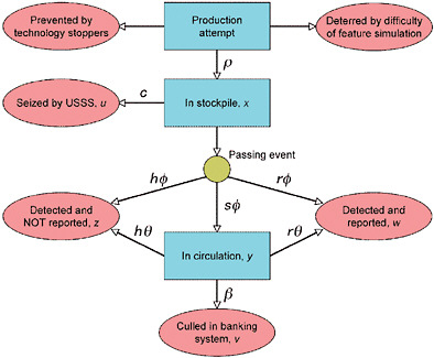
FIGURE E-1 A flow model for counterfeiting. The boxes indicate the components of the counterfeiting system. The ovals represent processes by which counterfeit notes are removed from the system. Arrows indicate the flow of counterfeit notes. NOTE: USSS = U.S. Secret Service. Variables are defined in Table E-1.
TABLE E-1 Variables in the Flow Model for Counterfeiting
|
Variables |
Definition |
|
Counterfeit repository (total $) |
|
|
u |
$ seized from stockpile by U.S. Secret Service (USSS) |
|
v |
$ culled from banking system by the Federal Reserve System (FRS) |
|
w |
$ turned in to USSS by a recipient |
|
x |
$ in stockpile, awaiting first pass attempt |
|
y |
$ in circulation |
|
z |
$ held by a recipient, but not reported or repassed |
|
Rates |
|
|
c |
Confiscation rate of notes from stockpile ($ per unit time) |
|
β |
Rate of culling in the banking system by the FRS (per unit time) |
|
|
Rate at which first attempts are made to pass note from stockpile (per unit time) |
|
θ |
Rate at which repass attempts are made during circulation (per unit time) |
|
ρ |
Counterfeit production rate ($ per unit time) |
|
Other parameters |
|
|
h |
Fraction of pass attempts held and not reported to the USSS; h = 1 − s − r |
|
r |
Fraction of pass attempts reported by recipient |
|
s |
Fraction of successful pass attempts |
|
t |
Time since start of production |
TABLE E-2 Differential, Time-Dependent, and Steady-State Flow Equations in the Flow Model for Counterfeiting
|
Repository |
Flow Rate In/Out of Repository |
Time-Dependent Amount in Repository |
Steady-State Amount in Repository |
|
x |
|
|
|
|
y |
|
|
|
|
z |
|
|
|
|
w |
|
|
|
|
u |
|
u(t)=ct |
|
|
v |
|
|
|
|
NOTE: Variables are defined in Table E-1. Note that for convenience, μ = (h + r)θ + β. |
|||
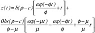
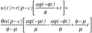
With these assumptions, the flows can be represented by first-order, linear ordinary differential equations that are straightforward to solve. Table E-2 also shows the time-dependent and steady-state (that is, t → ∞) solution for each repository. The steady-state solutions give the “average” amount of counterfeit currency in each of the counterfeit repositories. (Note that the steady-state solution for the removal repositories is necessarily infinite, since counterfeits only flow in and never out.) Of greatest interest are x(∞), the average amount of counterfeit in the stockpile waiting to be passed, and y(∞), the average amount of counterfeit in circulation. These are the amounts that arguably would be decreased by using effective features.
FEATURE ANALYSIS USING THE FLOW MODEL
For the sake of demonstrating the power of the flow model proposed, consider three potential features with different characteristics, as shown in Table E-3. For example, Feature A might use a metameric ink that can be easily simulated by a laser printing process but easily detected with a handheld device. Feature B might be similar to current security threads. Feature C might be a form of extreme microprinting, which is hard to duplicate but also hard to detect in a casual transaction.
A naïve comparison of these features might assign values on a scale of 0 to 2 and add values to determine an “effectiveness score” (see Table E-4). That the total score is the same for all three features points out the inherent dangers in using additive measures—something that might not be apparent with a larger, richer, and more complex set of criteria.
By contrast, it is possible to examine the three features using Equation (2-1) in Chapter 2. Assume, for convenience, that θ = 50 (that is, the average time between passing attempts is roughly 1 week), and that β = 10 (the average time to get swept up by a Federal Reserve Bank is roughly 1 month). In addition, assume that the stockpile confiscation rate c is proportional to the production rate ρ, so that c = kρ, where k is a constant of proportionality. Then Equation (2-1) becomes
(E-1)
TABLE E-3 Potential Features for Flow Model
|
Feature |
Difficulty of Simulation |
Detection Effectiveness |
|
A |
Low |
High |
|
B |
Medium |
Medium |
|
C |
High |
Low |
TABLE E-4 Demonstration of a Possible Assignment of Effectiveness Scores/Values
|
Feature |
Difficulty of Simulation |
Detection Effectiveness |
Total Effectiveness |
|
A |
0 |
2 |
2 |
|
B |
1 |
1 |
2 |
|
C |
2 |
0 |
2 |
TABLE E-5 A Nominal Characterization Table for the Comparison of Features A, B, and C
|
Feature |
Production Rate ρ |
Passing Fraction s |
Amount Circulating y(∞) |
|
A |
0.9 |
0.1 |
0.02 |
|
B |
0.5 |
0.5 |
0.07 |
|
C |
0.1 |
0.9 |
0.06 |
Comparison tables can now be developed to reflect the respective features’ effects on the remaining parameters s and ρ.1
To continue the hypothetical example, suppose a “nominal characterization” table could be used to assign values for s and ρ, as shown in Table E-5 (where the values of ρ are scaled so that ρ = 1 reflects the lowest difficulty to simulate, and ρ = 0 the highest).
Note that while the additive score for the parameters that measure difficulty of simulation (ρ) and detection efficiency (s) remains the same for all features, the steady-state amounts of counterfeits in circulation differ by more than a factor of three. According to this metric, Feature A is much more attractive than the other two: in this example, hindering passing is more important than deterring production in keeping counterfeits out of circulation. Interestingly, Feature B, which nominally deters both production and passing moderately well, gives the highest amount of counterfeits in circulation: at least in this example, it is more important to do one thing well than to do all things adequately.
One might ask, What is the effect of a note that does both things well? For a note design that deters production (ρ = 0.1) and hinders passing (s = 0.1), Equation (E-1) predicts a circulating amount y(∞) = 0.002, a factor of 10 less than for Feature A, which only does one thing well. Unsurprisingly, the best feature is one that deters both production and passing; therefore, in evaluating proposed features, the committee selected ones that scored well in both areas, as discussed in Chapter 4.
The flow model feature analysis encourages other investigations. For example, each class of counterfeiter will likely have different values of each variable (that is, both the production rate and pass frequency are likely higher for the professional than for the opportunist), and this affects where and how deterrence and enforcement measures are optimally applied. Thus, the flow model not only can provide a quantitative basis for deciding on and supporting features to develop, but it can serve as a means for directing research into the values of critical parameter values.
In particular, it would seem appropriate for the Bureau of Engraving and Printing (BEP) to engage in a series of large-scale field-like experiments in order to understand the “detectability” of various existing and proposed features.
The committee also observes that the model makes it obvious that machine authentication affects counterfeit flows only via culling in the banking system (given by the variable β). While counterfeit notes may pass through (and be rejected by) machine readers a number of times during circulation, these are almost always returned to the holder and remain in circulation until removed by a human or culled in the banking system. Therefore, machine readers only weakly affect r or h.
Finally, it should be clear that the hypothetical example presented in this appendix should not be interpreted to mean that the committee is suggesting that a single, dominant feature by itself would deter counterfeiting. The whole purpose of presenting a modeling approach is to provide a framework within which the effectiveness of combinations of features can be assessed in a consistent manner.


