
CHAPTER TWO
Goals for Limiting Future Climate Change
The purpose of this report is to suggest strategies for limiting the magnitude of future climate change. Although limiting climate change is a global issue, our assignment is to recommend domestic strategies and actions. A goal for reducing U.S. greenhouse gas (GHG) emissions is therefore needed as a basis for designing domestic policies, for evaluating their feasibility, and for monitoring their effectiveness. In this chapter, we examine how such goals can be set. We first assess future domestic and global “reference” GHG emission scenarios, that is, scenarios that would result without new policies to limit future emissions. We then outline the key steps involved in formulating goals for policies that limit climate change and recommend that goals be framed in terms of limits on cumulative domestic GHG emissions over a specified time period. In choosing a specific goal for the United States, policy makers will have to deal not only with scientific uncertainties but also with ethical judgments. Because the judgments can be informed but not fully answered by science, we do not attempt to recommend a specific U.S. emissions budget. However, in order to have a basis for identifying and evaluating policy recommendations, we have used recent modeling studies (most notably the EMF22 study1) to suggest a plausible range for a domestic GHG emissions budget. We then examine options for global and U.S. emissions-reduction goals, respectively, and finally we examine some potential economic impacts of these emission reduction goals.
REFERENCE U.S. AND GLOBAL EMISSIONS
The most recent data for U.S. GHG emissions (for the year 2007) show a total of 7,150 million CO2-equivalent tons (Mt CO2-eq).2 Over 85 percent of this total is CO2 emis-
|
1 |
Stanford University Energy Modeling Forum (EMF22; see http://emf.stanford.edu/research/emf22/ and Clarke et al., 2009). Although other models can be used, as explained in Box 2.2, we believe that EMF22 is particularly useful for our purposes and that the insights from EMF22 are consistent with the broader literature. |
|
2 |
A common practice is to compare and aggregate emissions among different GHGs by using global warming potentials (GWPs). Emissions are converted to a CO2 equivalent (CO2-eq) basis using GWPs as published by the Intergovernmental Panel on Climate Change (IPCC). GWPs used here and elsewhere are calculated over a 100-year period, and they vary due to the gases’ ability to trap heat and their atmospheric |
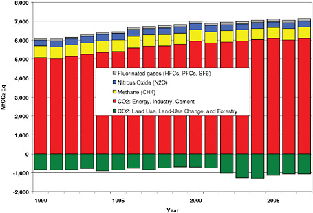
FIGURE 2.1 Historic U.S. greenhouse gas emissions and sinks. CO2 is the dominant GHG, but the contributions from other GHGs are not insignificant. SOURCE: EPA (2009).
sions, and roughly 94 percent of the CO2 emissions comes from combustion of fossil fuel (with most of the rest arising from industrial processes such as cement manufacturing). Methane (CH4) makes up about 8 percent of total emissions, nitrous oxide (N2O) about 4 percent, and the fluorinated gases (hydrofluorocarbons [HFCs], perfluorocarbons [PFCs], SF6) about 2 percent. There is also a net CO2 sink (removal from the atmosphere) from land-use and forestry activities, estimated at 1,063 Mt CO2 in 2007. Between 1990 and 2007, total U.S. GHG emissions have risen by 17 percent, with a relatively steady annual average growth of 1 percent per year. Figure 2.1 illustrates these trends (EPA, 2009).
The main drivers of GHG emissions include population growth and economic activity, coupled with the intensity of energy use per capita and per unit of economic output. Figure 2.2 shows that U.S. primary energy use has continued to grow over the
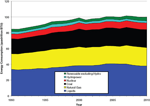
FIGURE 2.2 U.S. primary energy use, 1990 to 2010. Fossil fuels are the dominant energy source over this period. “Liquids” refers petroleum products including gasoline, natural gas plant liquids, and crude oil burned as fuel, but it does not include the fuel ethanol portion of motor gasoline. SOURCE: EIA (2009).
period of 1990 to 2010, although at a decreasing rate: Total energy consumption has grown at a slower pace than economic output and population. This slower growth in energy consumption stems from structural changes in the U.S. economy (e.g., the shift to a more service-oriented economy) as well as increasing energy efficiency per unit of economic output. Trends in GHG emissions are closely associated with energy consumption. Figure 2.3 compares growth in GHG emissions with growth in primary energy use, population, and economic output in the United States. Since 1990, the U.S. economy has doubled in size while the population has grown about 20 percent and energy use and GHG emissions have grown 10 to 15 percent (EPA, 2009). Recent government projections out to 2030 are for economic growth to continue along historic rates, outpacing growth in energy use and GHG emissions because of the reduced energy intensity of the economy.
![FIGURE 2.3 Historical trends and projected future trends in U.S. GHG emissions (including CO2, CH4, N2O, HFCs, PFCs, and SF6, but excluding net land-use emissions) and indices of key emission drivers: population, primary energy use, and economic growth (gross domestic product [GDP]). GHG emissions have risen roughly in concert with growth in energy use and population, but substantially slower than the rate of overall economic growth. The base year for calculating the indices is 1990. GDP estimates used to calculate the GDP index are based on real 2005 U.S. dollars. SOURCES: Historic data are from EPA (2009) and CEA (2009); projected data are from the ADAGE model (EPA, 2009).](/openbook/12785/xhtml/images/p2001c3c3g24001.jpg)
FIGURE 2.3 Historical trends and projected future trends in U.S. GHG emissions (including CO2, CH4, N2O, HFCs, PFCs, and SF6, but excluding net land-use emissions) and indices of key emission drivers: population, primary energy use, and economic growth (gross domestic product [GDP]). GHG emissions have risen roughly in concert with growth in energy use and population, but substantially slower than the rate of overall economic growth. The base year for calculating the indices is 1990. GDP estimates used to calculate the GDP index are based on real 2005 U.S. dollars. SOURCES: Historic data are from EPA (2009) and CEA (2009); projected data are from the ADAGE model (EPA, 2009).
Figure 2.4 provides a range of recent GHG emission scenarios from various models (EIA, 2009; Fawcett et al., 2009) assuming no mitigation policies are in place. The chart shows that emissions in 2030 range from 7,100 to 8,400 Mt CO2-eq and in 2050 range from 8,100 to 10,900 Mt CO2-eq. Variations in projections are the result of varying assumptions of economic growth, energy efficiency, and the deployment of energy technologies (all in the absence of national GHG emissions-reduction policies). For example, MIT’s EPPA model assumes an annual GDP growth rate of 2.5 percent per year from 2005 to 2050 (Paltsev et al., 2009), while the Electric Power Research Institute’s (EPRI’s) MERGE model assumes lower annual growth rates starting at 2.2 percent through 2020 and declining to 1.3 percent through 2050 (Blanford et al., 2009). In addition, the MERGE model assumes a movement away from oil and toward more electric generation as a
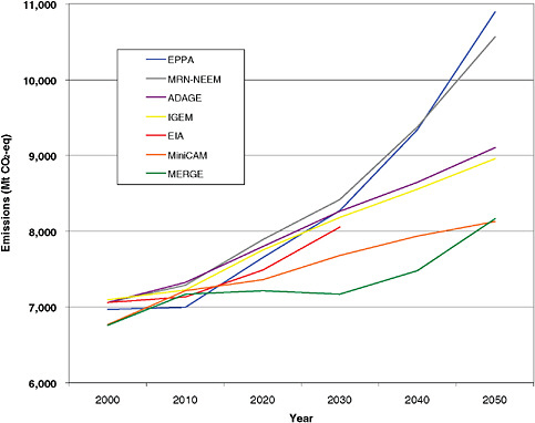
FIGURE 2.4 Reference (“no policy”) GHG emission scenarios including CO2, CH4, N2O, HFCs, PFCs, and SF6. These scenarios include source emissions across many sectors but exclude net emissions from land use–related carbon sequestration. Despite the wide range of outcomes among the different projections, they all show increasing emissions over time. The Applied Dynamic Analysis of the Global Economy (AD-AGE) model results are the same as the GHG emissions line used in Figure 2.3. SOURCES: Adapted from Fawcett et al. (2009) and EIA (2009).
share of energy use. The combined assumptions of lower economic growth and less carbon-intensive energy use produce lower GHG emissions in the MERGE reference projection. Recognizing the inherent uncertainty associated with making long-term projections, two key insights emerge from the reference projections:
-
In the absence of emission mitigation policies, annual U.S. GHG emissions will continue to increase out to 2050 (even as the energy intensity of the economy declines).
-
The earlier that measures are taken to influence the trajectory of emissions, the more long-term emissions can be reduced.
Similar to U.S. projections, global projections of GHG emissions are determined by the dynamic interaction of key emissions drivers, most notably population and economic growth, as well as the intensity of energy use (per capita and per unit of economic output) and technological change. Projections of GHG drivers, emissions, and concentrations are taken from the recent EMF22 study (Clarke et al., 2009). Figure 2.5 provides recent population projections from models participating in the EMF22 study. The mean of the global population estimates for 2010 is about 7 billion people. Global population projections for 2050 have a mean of about 9 billion people. In all of the employed reference models, population growth rates are projected to slow toward the end of the 21st century, producing a mean projection of 9.5 billion people in 2100 but a wide variability among the models (from 8.7 to 10.5 billion people). Such variability among models can be expected, since long-range global population projections embody different assumptions about regional population trends. For example, trends
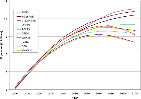
FIGURE 2.5 Reference global population projections from the models used in the EMF22 study. The divergence among the different model projections grows over time. SOURCE: L. Clarke, Pacific Northwest National Laboratory (PNNL).
in sub-Saharan Africa, the Middle East and North Africa, and the East Asia regions are driven by changes in lower-than-expected fertility rates based on recent data. In the Organisation for Economic Co-operation and Development (OECD) region, by contrast, recent projections are somewhat higher than previous estimates mainly due to changes in assumptions regarding migration and more optimistic projections of future life expectancy.
The reference projections for global primary energy consumption from the EMF22 study are shown in Figure 2.6. The range of global energy production in 2050 is between 790 and 1,115 exajoules3 with a mean value of about 890 exajoules. The rates of growth in primary energy consumption are greater than population growth, leading to an even greater per capita energy use out to 2100. By the end of the century, global energy production is projected to be between 2.5 and 3.5 times greater than today’s levels. The key reasons for differences in total primary energy projections include assumptions about population and economic growth; improvement in energy intensity, that is, the relationship between energy consumption and economic output over time; the abundance of different fuels and their relative prices; and the availability and deployment of energy technologies. For example, a scenario that projects more coal use will result in more CO2 emissions than one where natural gas and renewable energy represent a larger share of total energy consumption.
Figure 2.7 shows global projections of fossil and industrial CO2 emissions and the CO2-eq concentrations4 from all Kyoto Protocol gases (CO2, CH4, N2O, HFCs, PFCs, and SF6) from the EMF22 reference (no policy) scenarios (Clarke et al., 2009). Reference projections of global GHG emissions and concentrations highlight the fact that global emissions and concentrations will increase substantially over the century, with attendant changes in the global climate. There is a wide spread in emissions projections, resulting from many of the same uncertainties that are reflected in the primary energy projections, along with uncertainties about the development and deployment of low-carbon energy technologies without mitigation policy. Regardless, the projections all indicate upward trends. By the end of the century, the range of CO2-eq concentrations spans from two times to almost four times today’s levels. (That is, concentrations in
|
3 |
Primary energy is energy contained in raw fuel that has not been subjected to any conversion or transformation process. One exajoule = 1018 joules. A joule is the work required to continuously produce one watt of power for one second. |
|
4 |
CO2-eq (CO2 equivalent) concentration is defined as a multi-GHG concentration that would lead to the same impact on the Earth’s radiative balance as a concentration of CO2 only (IPCC, 2007b). See Box 2.1 for further discussion. |
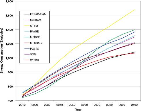
FIGURE 2.6 Reference global primary energy consumption projections from the models used in the EMF22 study. Note that all estimates project considerable growth in energy production over the course of the century. SOURCE: Adapted from Clarke et al. (2009).
2050 range between 800 and 1,500 ppm5 CO2-eq, in contrast to today’s concentrations of roughly 440 ppm CO2-eq.)
Although the high-income (OECD) countries are currently the largest contributors to cumulative GHG emissions, emissions from rapidly growing low- and middle-income countries (e.g., Brazil, China, and India) are projected to grow more quickly than those of high-income countries. Figure 2.8 shows historical and projected contributions to global emissions out to 2100 from several sources. In all the projections, the balance of cumulative GHG contributions shifts from the high-income to the low- and middle-income countries through 2050; in second half of the 21st century, the low- and middle-
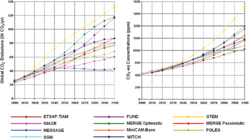
FIGURE 2.7 Projections of global CO2 emissions (from fossil and industrial sources) and CO2-equivalent concentrations (CO2-eq) in the absence of efforts to address climate change, from the EMF22 study. The left panel shows global (fossil and industrial) CO2 emissions from across models. The right panel shows the CO2-eq concentrations, including all the Kyoto Protocol gases, for the same corresponding scenarios. Model projections vary, but all show increasing emissions and concentrations over time. See Box 2.1 for definition of CO2-eq concentrations. SOURCE: L. Clarke, PNNL.
income countries are projected to account for the bulk of cumulative global GHG emissions.
Together, these factors frame the international context in which the United States will need to decide on its domestic emissions-reduction goals, and also on its support for and involvement in international actions. Even today, as one of the largest individual GHG emitters, the United States cannot substantially reduce global emissions through unilateral action. With its shrinking relative contribution to global emissions, unilateral action by the United States would be decreasingly effective from a quantitative perspective. In some sense, then, a primary role of U.S. action in climate change is to provide global leadership and to motivate effective international action. See Chapter 7 for a fuller discussion of these issues.
SETTING CLIMATE CHANGE LIMITING GOALS
International policy goals for limiting climate change were established in 1992 under the UNFCCC, in which the United States and more than 190 other nations set the goal of “stabilization of GHG concentrations in the atmosphere at a level that would prevent dangerous anthropogenic interference with the climate system.” Subsequent scientific research has sought to better understand and quantify the links among GHG emissions, atmospheric GHG concentrations, changes in global climate, and the impacts of those changes on human and environmental systems. Based on this research, many policy makers in the international community recognize limiting the increase in global mean surface temperature to 2°C above preindustrial levels as an important benchmark; this goal was embodied in the Copenhagen Accords, at a 2009 meeting of the G-8, and in other policy forums.
Although these temperature and concentration goals are essential metrics for limiting global climate change over time, they are not sufficient to guide near-term, domestic policy goals. Policy requires a goal linked to outcomes that domestic action can directly affect and that can be measured contemporaneously. Global temperature and concentration goals lack this attribute, because they are the consequence of global, and not just domestic, actions to limit GHG emissions. To avoid this problem, a limit on cumulative emissions from domestic sources, measured in physical quantities of GHGs allowed over a specified time period, is in the panel’s view a more useful domestic policy goal. Policy can affect emissions directly, and actual emissions can be measured reasonably accurately on a current basis.
Calculating the U.S. emissions budget is conceptually straightforward, but it involves a number of uncertainties and judgments that are complex and potentially contro-
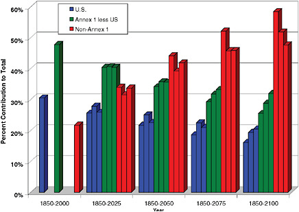
FIGURE 2.8 Historical and future contributions to global CO2 emissions from fossil and industrial sources (does not include net CO2 emissions from land use). Annex I and non-Annex I refer to high-income and low- and middle-income groups of countries, respectively, under the UNFCCC. The three bars for each color within each time period represent emissions projections from three models used in the U.S. Climate Change Science Program (CCSP) studies: MIT’s EPPA model, EPRI’s MERGE model, and PNNL’s MiniCAM model. Note that the United States and other high-income countries have had the dominant share of emissions historically, but this share is projected to decrease over time. SOURCES: Historical estimates from Climate Analysis Indicators Tool, Version 6 (WRI, 2009); projections are from U.S. CCSP 2.1a (Clarke, 2007).
versial. To systematically derive an emissions budget from global temperature and concentration goals requires establishing three crucial links:
-
a target global atmospheric GHG concentration that is consistent with an acceptable global mean temperature change,
-
a global emissions budget that is consistent with a target atmospheric GHG concentration, and
-
an allocation to the United States of an appropriate share of the global emissions budget.
According to the most recent assessment of the IPCC, the best estimate of global mean temperature increase over preindustrial levels resulting from stabilizing at-
mospheric GHG concentrations over the long term at 450 CO2-eq is 2°C;6 the best estimate of temperature increase resulting from stabilizing atmospheric GHG concentrations at 550 CO2-eq is 3°C (Meehl and Stocker, 2007). However, as discussed in Box 2.1, linking global temperature change with a target GHG concentration involves a number of physical processes that are not fully understood; thus, there is substantial uncertainty surrounding this linkage. For example, a 450 ppmv CO2-eq concentration could be associated with temperature change below 2°C or well above 2°C (Meehl and Stocker, 2007). Future research may change prevailing views about desired temperature change limits or the atmospheric GHG concentration for achieving these temperature limits. Nonetheless, for the purposes of this report, we use these two concentrations (450 and 550 CO2-eq) as guideposts for considering global emissions budgets and U.S. emissions allocations. The following two sections address these linkages.
The next step of the goal-setting process—allocating an appropriate share of the global budget to the United States—is also a matter of considerable uncertainty and judgment. While science may inform this judgment, it depends mostly on ethical and political considerations (e.g., debates over whether allocation criteria should be based on economic efficiency criteria or on “fairness” criteria). For these reasons, we do not attempt to recommend a specific domestic emissions budget. We do, however, draw upon the work of the EMF22 modeling exercises (see Box 2.2), which identifies specific domestic emissions budget scenarios that are linked to various global action cases. We have adopted the EMF22 results as representative emission targets, both to illustrate an approximate range into which a U.S. budget might fall and to provide some sort of benchmark for evaluating the technical feasibility of reaching a budget target. We discuss the EMF22 results in the following section.
GLOBAL EMISSION TARGETS
EMF22 modeled reference scenarios to provide a range of possible paths of emissions growth under the assumption of no new climate policies. Figure 2.7 shows this range (based on forcing from the Kyoto gases only) and shows that the 450 and 550 CO2-eq limits will soon be exceeded without aggressive and immediate new emission reduction efforts. To explore what sort of actions might be required in this regard, EMF22 evaluated 10 international climate-action cases, based on combinations of three key elements of a long-term GHG emissions-reduction strategy: (1) long-term concentra-
tion goals, using either 450, 550, or 650 CO2-eq; (2) whether the concentration goal could be exceeded before the end of the 21st century (overshoot or not-to-exceed); and (3) the assumption of international participation—either full participation, meaning all countries undertake emissions-reduction efforts starting in 2012, or delayed participation, meaning low- and middle-income countries do not begin emissions-reduction efforts until 2030 or beyond. Figure 2.9 presents the global fossil and industrial CO2 emissions in 2050, relative to 2000 levels, resulting from the scenarios analyzed in the EMF22 international study. In each of the cases, resulting emissions are well below what they would be without the implementation of climate change limiting polices.
It is important to keep in mind that these are simply scenarios, and they do not represent all the ways that particular goals could be achieved. In particular, the models are based on a “least-cost” approach to emissions-reduction efforts, which assumes that all nations undertaking emissions-reduction efforts do so in the most cost-effective manner (i.e., emissions reductions undertaken where, when, and how they will be least expensive), under the equivalent of a frictionless cap-and-trade system with full international trading covering all Kyoto gases. One implication of this least-cost approach is that some sectors or countries will undertake more or less mitigation than others. In addition, the models assume transparent markets, no transaction costs, and perfect implementation of emissions-reduction measures throughout the 21st century. At the same time, the delayed participation scenarios assume a highly inefficient architecture in which many of the low- and middle-income countries undertake no emissions reductions before 2030 or even 2050.
The more stringent climate-action cases (including the 450 ppm CO2-eq cases and the 550 ppm CO2-eq case without immediate, full global participation) could not be represented in some or all models. These are shown at the bottom of Figure 2.9.7 This does not necessarily imply that these climate-action cases are impossible in some absolute sense; rather, it is one of several indicators of the challenges of meeting the particular goals under the particular constraints that are represented by a given climate-action case. In general, the difficulty of successfully modeling scenarios increased with the stringency of the long-term goal, with the requirement not to exceed the goal dur-
|
BOX 2.1 Key Uncertainties in Setting Goals for Limiting Climate Change The report ACC: Advancing the Science of Climate Change (NRC, 2010a) provides a detailed discussion of the scientific uncertainties involved in setting targets for limiting climate change. Here we provide a brief overview of some key uncertainties that affect the results presented later in this chapter. Climate sensitivity. The quantitative relationship between long-term temperature changes and atmospheric GHG concentrations is very difficult to specify, due primarily to the large uncertainty of climate sensitivity. Climate sensitivity is typically defined as the global mean equilibrium temperature response to a doubling of CO2 concentrations. IPCC (2007b) indicated that climate sensitivity is likely to be in the range of 2°C to 4.5°C with a best estimate of about 3°C. It is very unlikely to be less than 1.5°C,1 and values substantially higher than 4.5°C cannot be excluded. Some recent studies have in fact suggested that much higher climate sensitivity values are possible (Hansen et al., 2008; Sokolov et al., 2009). This uncertainty indicates that relying only on the best estimate of 3°C may not be a prudent risk-management strategy. Because of these uncertainties, the temperature-concentration relationship is often given in probabilistic terms. As noted earlier, recent research (Meehl and Stocker, 2007; Wigley et al., 2009) indicates that limiting global GHG concentrations to around 450 ppm CO2-eq over the long term would result in a 2°C temperature change using a climate sensitivity of 3°C. The best-estimate increase in temperature for a long-term concentration of 550 ppm CO2-eq is 3°C (or 2°C, if the climate sensitivity is at the lowest end of the IPCC range). However, there is significant uncertainty around these point estimates. For example, a study using three models from the EMF22 exercise finds that the probability of staying below 2°C for several “overshoot” scenarios (see below) leading to 450 ppmv CO2-eq ranges between 24 and 72 percent, depending on the degree of overshoot and on which probability distribution from the literature is used (Krey and Riahi, 2009). A related consideration is that, due to time lags in the climate system, one might allow actual concentrations to temporarily and modestly exceed (or “overshoot”) 450 ppm CO2-eq while allowing temperature to remain below the 2°C temperature goal. However, an overshoot scenario entails ad |
ing the century, and with delays in full global participation. For instance, only 2 of the 14 participating models8 were able to produce scenarios that attained the 450 CO2-eq goal without immediate, full global participation, and only then if an overshoot trajectory to the goal was allowed. Without the option to overshoot the goal, and with
|
ditional climate risks that depend on how the climate system responds to concentrations above 450 ppm CO2-eq. For instance, this could send the climate system over critical thresholds (e.g., irreversible drying of the subtropics, melting large glaciers, and raising sea levels); once such thresholds are crossed, reducing CO2-eq concentrations may be ineffective for bringing the climate system back to a particular state (Solomon et al., 2009). Finally, allowing emissions to follow an overshoot pathway in the near term leaves open the possibility that, once the concentration target is exceeded, the necessarily steeper emissions declines later in the century may never materialize. Radiative forcing and CO2-eq concentrations. Radiative forcing is a measure of impact on the Earth’s radiative balance from changes in concentrations of key substances such as GHGs and aerosols. It is generally expressed in terms of watts per meters squared (W/m2) but can also be expressed in terms of CO2-equivalent(CO2 -eq) concentrations, that is, the concentrations of CO2 only that would lead to the same impact on the Earth’s radiative balance (Ramaswamy et al., 2001). Radiative forcing agents in the atmosphere that are most relevant to considerations of future climate change include the “Kyoto” gases (those included in the Kyoto Protocol: CO2, CH4, N2O, HFCs, PFCs, and SF6); CFCs and other ozone-depleting substances covered by the Montreal Protocol; tropospheric ozone; different types of aerosols including sulfates, black carbon, and organic carbon; and land use changes that affect the reflectivity of the Earth’s surface. Many global emissions scenarios consider only CO2 or only the Kyoto gases. The results of analyses that include only Kyoto gas forcing differ from those that include “full forcing,” primarily due to the impact of aerosols. The aerosol influence is complex; some types such as black carbon exert positive forcing (warming), while other types such as sulfates exert negative forcing (cooling). It is estimated that, overall, aerosol-related cooling influences currently lower total forcing by roughly an equivalent of 50 ppm CO2 (Forster and Ramaswamy, 2007). Many studies indicate that the aerosol influence will attenuate over the coming century, however, particularly if strong climate change limiting policies are enacted. This is because aerosol emissions from fossil fuel combustion are expected to be significantly reduced, both as an indirect result of GHG mitigation efforts and as a direct result of concerns over health impacts. For example, in scenarios from the EMF22 models that most comprehensively considered full forcing, it was found that, by the end of the century, Kyoto-only CO2-eq concentrations were roughly equal to full-forcing concentrations. |
delays in global participation, no models could produce the scenario that met 450 ppm CO2-eq by 2100.
The EMF22 results indicate that atmospheric GHG concentrations can be kept below 450 ppm CO2-eq only if the United States and other high-income countries, along with China, India, and many other low- and middle-income countries around the world, take aggressive actions to reduce emissions starting within the next few years. This would represent a dramatic change from recent trends across the globe. If the major
|
BOX 2.2 Our Use of EMF22 To identify plausible goals for a U.S. GHG emissions budget, and to evaluate strategies for meeting this budget, we have relied largely on the work of Energy Modeling Forum Study 22 (EMF22). EMF22 included two components that are relevant here: an international component that engaged 10 of the world’s leading integrated assessment models to assess global climate regimes (Clarke et al., 2009) and a U.S. component that engaged six models to assess U.S. emissions goal options (Fawcett et al., 2009). There are other modeling studies and projections that one could consider, but we found EMF22 to be particularly useful for a number of reasons:
|
developing regions delay action by a few decades, then the 450 ppm CO2-eq goal could be met only by the end of the century if concentrations are allowed to temporarily overshoot this goal.
U.S. EMISSION TARGETS
U.S. GHG emissions reductions will not by themselves have a decisive impact on global atmospheric GHG concentrations, but actions that the United States might take over the coming decades to reduce domestic emissions do need to be considered within the context of the ultimate goal of stabilizing global climate. To this end, the EMF22 U.S. study (Fawcett et al., 2009) calculated different cumulative U.S. GHG emission budget goals over the period 2012 to 2050, based on the selection of a base year and a corresponding emissions-reduction target to be achieved by 2050 (Table 2.1). They calculated that an 80 percent reduction from 1990 levels corresponds to a budget of
We know of no other recent modeling exercise that exhibits all these useful features. Nevertheless, we also recognize some important limitations of the EMF22 study. These include, for instance, the question of how aerosols and land use impacts are represented in the models. We note in the subsequent sections where these limitations affect our analysis, but overall we do not believe these effects significantly change our main conclusions and recommendations. |
167 gigatons (Gt) CO2-eq9 (and a 50 percent reduction corresponds to a budget of 203 Gt CO2-eq10). Table 2.1 illustrates that the budget values do not change a great deal if different baseline years are selected. This is a useful characteristic of a cumulative budget, since the choice of baseline year is often an issue of contentious debate in policy negotiations.
We chose to round these EMF numbers and adopt a cumulative emissions budget in a range of 170 to 200 Gt CO2-eq over the period 2012-2050 as a reasonably representative U.S. budget target, which can serve as a benchmark for developing policy recommendations and testing their feasibility. This budget range, which represents a significant change from business-as-usual U.S. emissions out to 2050, is roughly in line with the types of emissions-reduction goals found in many recent policy propos-
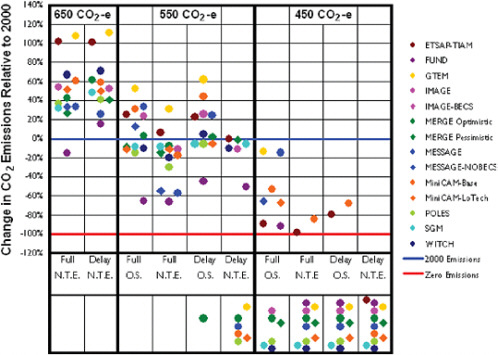
FIGURE 2.9 Global fossil and industrial CO2 emissions in 2050 relative to those in 2000. Long-term concentration goals are 450, 550, or 650 CO2-eq (Kyoto gases). The level of international action is either “Full,” meaning all countries undertake emissions mitigation starting in 2012, or “Delay,” meaning low- and middle-income countries do not begin climate mitigation until 2030 or beyond. The option to exceed or “overshoot” the long-term concentration goal this century was defined either as a not-to-exceed formulation (N.T.E. in the figure) or as an overshoot case (O.S.). The more stringent scenarios (starting with the 550 ppm CO2-eq case, without immediate global participation), could not be represented in some or all models and are indicated as such at the bottom of the figure. SOURCE: Clarke et al. (2009).
TABLE 2.1 Cumulative U.S. GHG Emissions (Gt CO2-eq) for the Period 2012 to 2050, Assuming Linear Emissions Reductions Throughout That Time Period, Beginning at a 2008 Emissions Level, and Assuming 100 Percent Coverage of GHG Emissions in the Economy
|
Base Year |
Percent Below Base Year Emissions in 2050 |
||||||
|
83% |
80% |
65% |
50% |
35% |
20% |
0% |
|
|
1990 |
164 |
167 |
185 |
203 |
221 |
239 |
262 |
|
2005 |
167 |
171 |
192 |
213 |
234 |
254 |
282 |
|
2008 |
168 |
172 |
194 |
215 |
237 |
258 |
287 |
|
SOURCES: Fawcett et al. (2009). Emissions data from 1990 and 2005 are from EPA (2009), and 2008 emissions projections are based on Paltsev et al. (2007). |
|||||||
als. See Figure 2.10 for a graphical representation of these goals. Note that these goals are presented as limits for cumulative U.S. domestic emissions (rather than goals to be met through international offsets). Excluding some sectors from emissions reductions, or allowing international and domestic offsets, could substantially alter the actual U.S. emissions reductions.
This budget range also relates usefully to the EMF22 international scenarios, where modeling results for global emissions reduction were disaggregated (using the global least-cost criteria described earlier) to indicate the degree of U.S. action associated with global goals under differing cases of international action (the same set of cases illustrated in Figure 2.9). The results show a considerable range of possible U.S. contributions, reflecting the large uncertainties inherent in any long-range (midcentury) projections. In general, however, the EMF22 results indicate that a 200 Gt CO2-eq U.S. budget is roughly consistent with a long-term global goal of 550 ppm CO2-eq, particularly if there is full international participation. This same U.S. budget could also be consistent with long-term global goals of 450 ppm CO2-eq, but only if the option exists to overshoot the goal (with the attendant requirement for more aggressive actions beyond 2050) and if there are also immediate, aggressive, and comprehensive global GHG emissions-reduction efforts. The more stringent 170 Gt CO2-eq U.S. budget is roughly consistent with the 550 ppm CO2-eq global goals without overshoot or with delayed participation—or with the most idealized of the 450 ppm CO2-eq goals (immediate, comprehensive international action, and the opportunity to overshoot the long-term goal prior to 2100). See Clarke et al. (2009) and Fawcett et al. (2009) for further details on these calculations.
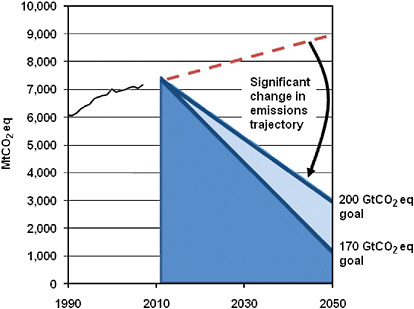
FIGURE 2.10 Illustration of the representative U.S. cumulative GHG emissions budget targets: 170 and 200 Gt CO2-eq (for Kyoto gases) (Gt, gigatons, or billion tons; Mt, megatons, or million tons). The exact value of the reference budget is uncertain, but nonetheless illustrates a clear need for a major departure from business as usual.
As mentioned above, these emissions budgets are for gross emissions in the United States and do not include sources and sinks from land use, land-use change, and forestry (LUCF). If LUCF emissions are net positive (emissions), it will make attaining these budgets more difficult. If LUCF emissions are net negative (sinks), which is the current trend, it will make attaining these budgets easier.
There are many differing views on the relative burdens that different countries should bear to address climate change. For example, it has been suggested that the United States should make more stringent emissions-reduction efforts, based, for instance, on precautionary concerns that lower global concentration targets are needed, or based on “fairness” arguments that high-income countries, having produced most of the GHG emissions to date, should shoulder a larger share of future emission reductions. For example, the German Advisory Council on Global Change (2009) developed a global emissions budget and applied the criterion of equal per capita emissions among all
countries; this calculation allocates to the United States a budget of 35 Gt CO2-eq over the same time period of the EMF22 budget.
Conversely, actions by other countries influence the U.S. contribution required to meet any global concentration goal. The EMF study indicates that, in general, the effect of delaying action is not to dramatically alter global emissions reductions required for 2050 but rather to cause a shift in the distribution of emissions among regions. Thus, emissions reductions not undertaken by one large country (or group of smaller countries) must be made up for by other countries in order to achieve atmospheric GHG stabilization at the levels explored in the scenarios above.
If the United States elected to make additional commitments beyond the least-cost allocated domestic budget mentioned above, it would be reasonable to achieve these additional commitments through a mechanism for investing in emissions reductions elsewhere in a way that does not increase the total cost of meeting the global emissions budget. The purchase of international offsets or participation in a global carbon pricing system would in principle provide such a mechanism. As discussed in Chapter 4, however, these mechanisms must be designed to ensure the emissions reductions are “real, additional, quantifiable, verifiable, transparent, and enforceable” and do not result in emissions leakage, all of which are difficult challenges to address.
If the United States sought to lessen its domestic emissions-reduction requirements by purchasing offsets from other countries, then to avoid double counting, the countries selling offsets could not take credit for these emissions reductions if they establish their own national emissions budget. Economic theory suggests that the solution to this kind of problem is to compensate the seller for the loss of the purchased emissions reduction. For example, the United States might purchase an offset from Country A for the price of the offset itself plus the future cost that Country A may face in reducing its emissions through actions that are more costly than the original offset. It is beyond our scope to recommend how to design an international offset system that addresses this issue, but it is worth noting that a system without this form of additional compensation may be resisted by countries interested in selling offsets.
Finally, we note that, because of the uncertainties and judgment involved, the initial U.S. domestic emissions budget may not be stable over time. Indeed, changes to the emissions budget—up or down—are to be expected. This is an unavoidable problem with a scientifically complex, politically controversial, and long-term problem like climate change. This fact is a primary reason for ensuring that the U.S. policy framework for limiting GHG emissions is both durable and adaptive, as discussed in Chapter 8.
IMPLICATIONS OF U.S. EMISSION GOALS
To evaluate the implications of the representative U.S. emissions budgets discussed above, we have drawn from the U.S. component of the EMF22 study11 (Fawcett et al., 2009). These analyses help illustrate one of the reasons why cumulative emissions goals are an effective way to set long-term targets: They allow flexibility in emissions over time. Emitters might either bank permits (by reducing more than the target in a particular year) or borrow permits (so that they can emit more than they are allotted in a given year). The opportunity to bank emissions rights for future use, or to borrow emissions rights from the future, means that the actual emissions pathway to any cumulative 2050 goal will probably not be linear (see Fawcett et al. [2009] for discussion of the forces that could influence the degree to which emitters choose to bank or borrow emissions rights).
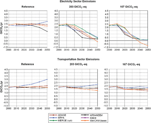
Figure 2.11 shows estimates from the same study for CO2 emissions reduction from electric power generation and transportation. For the 203 and 167 Gt CO2-eq scenarios, electricity sector emissions in 2050 are reduced by an average of approximately 90 and 100 percent, respectively; in the transportation sector, emissions fall by an average of approximately 20 and 30 percent, respectively. Overall, the electricity sector reduces emissions to levels well below the target while transportation-sector emissions remain well above the target. This reflects differences in the emissions-reduction options across sectors. These projections are of course influenced by assumptions built into the models, which are generally based on technologies and processes that we know how to characterize. It is possible that unknown technological breakthroughs or major socioeconomic shifts could lead to a very different picture in the future.
Ideally, the costs of U.S. emissions reductions are measured as a change in the well-being of Americans. However, all measures that aggregate across the entire population give rise to ethical questions about how to weigh differences in the well-being of separate individuals and groups within that population. Hence, for practical purposes, aggregate economic metrics are often used to represent the change in well-being that is brought on by emissions reductions. Typical metrics include CO2 prices (which, while not a direct measure of cost, can be used to determine effects on basic energy goods such as gasoline or natural gas for home heating and cooking) and overall changes to economic output such as GDP.
Figure 2.12 shows the carbon prices estimated in the U.S. component of the EMF22
study for the cumulative emissions scenarios discussed above. Several insights emerge: First, there is a distinct range of prices. For example, under the 167 Gt CO2-eq goal, the 2020 carbon price ranges from roughly $50 to $120 per ton of CO2. The differences among these estimates stem largely from differing expectations about the technologies that will be available and the ability to deploy these technologies effectively. Note that this includes not just energy supply technologies but also technologies to reduce emissions in end-use and industrial applications. Second, the effect of CO2 prices on energy gives a sense of the economic burden that would be imposed by emissions-reduction policies. Ultimately the effect of CO2 prices is to increase the cost of carbon-intensive energy and of products that use energy as an input. Table 2.2 shows the effect of a $100 per ton CO2 price on the costs of key fuels.
In all the scenarios and for all the models, carbon prices exhibit a steady increase. This is a key feature found in virtually all emissions-reduction studies. Because the stringency of the reductions must increase over time as emissions are eventually driven toward zero, the costs must go up over time. Thus, meeting the sorts of cumulative goals proposed here will require an increasing commitment with an increasing cost. Note, however, that increasing prices are based on the assumption that the exact degree and nature of future improvements in important drivers such as technology, economic growth, and population growth are known with certainty. If, for example, technology were to advance substantially more rapidly than expectations (for example, if there were to be a radical technological breakthrough), the CO2 price would rise less aggressively. Conversely, less-than-expected technological advance could drive price increases even higher. (See Chapter 5 for more discussion about technological innovation as a key factor for modulating GHG emission-control costs.)
Aggregate economic indicators such as GDP or consumption losses are another common way to represent the costs of GHG emissions reduction. Given the simplifications required for a model to represent the national economy, these sorts of estimates are best viewed as informative in relative terms but highly uncertain in absolute terms. Figure 2.13 shows projected U.S. GDP under reference cases and the two budget scenarios, looking across the different models used in the EMF22 study. There is a large degree of uncertainty in future economic growth, for instance, with reference projections for 2030 varying by about 22 percent from the highest to lowest estimated values.
An important insight emerges when comparing projected economic growth in a “no-policy” case (i.e., reference scenario) to a “policy” case (i.e., with mandates for the budget targets discussed earlier); that is, although climate action does put downward pressure on economic growth, the effects over the next several decades are generally
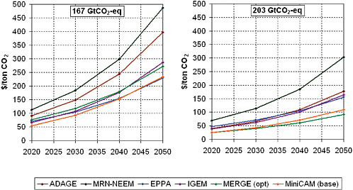
TABLE 2.2 Effect of Carbon Prices on Energy Prices
modest in comparison to the degree of growth. For instance, in the most optimistic projection of the EMF22 study, for the reference case, economic growth for the period 2010 to 2130 increases by 88 percent. When the most stringent emissions-reduction targets are imposed, economic growth still increases by 83 percent. In the most pessimistic projection, economic growth is 52 percent in the reference case; this is changed to 51 percent for the 167 Gt CO2-eq target case. Economic losses increase over time, so the expectation is that they will be larger through and beyond 2050 than they are through 2030. It is important to note that none of these GDP impacts include estimates of the welfare benefits that would be associated with reducing GHG emissions. Note also that these studies assume efficient national policy architectures resembling an economy-wide cap-and-trade system or carbon tax. Less efficient approaches could substantially increase costs.
Figure 2.14 presents another way of evaluating differences across models: to compare the impacts as a percentage of reference GDP. By 2030, GDP losses range from 0.5 to 4.5 percent. The range of estimates highlights the tremendous uncertainty surrounding the costs of climate action, which is due to differences among analyses including different economic growth and GHG emission levels in the reference (no-policy) case, differences in how households respond to higher energy prices, and variations in the deployment and effectiveness of mitigation technologies. This range is roughly consistent with previous studies, such as the U.S. CCSP scenarios (Clarke, 2007). In no scenario does growth stop or does the economy decline; rather, in all cases, the effect of the emissions-reduction policy is to delay the achievement of higher GDP levels. As
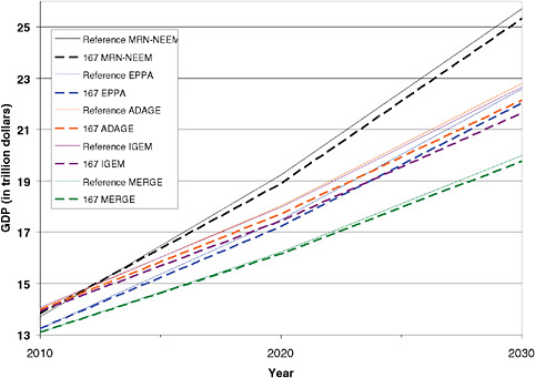
FIGURE 2.13 Projected U.S. GDP under reference cases and a 167 Gt CO2-eq budget goal across five models used in the EMF22 study. SOURCE: F. de la Chesnaye, EPRI.
noted above, none of these GDP impacts includes estimates of the benefits that would be associated with reducing GHG emissions.
A Congressional Budget Office report on the economic effects of GHG limiting policies (CBO, 2009) arrives at the same finding: that there is an upfront cost to the economy, but it will be relatively modest. The main impact of GHG limiting policies would be on energy expenditures, which accounted for about 9 percent of GDP in 2006 (EIA, 2009). A resulting price on GHG emissions ($/tCO2-eq) would lead to higher delivered-energy prices which in turn would lead to decreased economic output. In general, the economy will shift production, investment, and employment away from sectors related to the production of carbon-based energy and energy-intensive goods and services and toward sectors related to the production of alternative energy sources and non-energy-intensive goods and services.
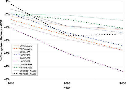
FIGURE 2.14 Impact of 167 and 203 Gt CO2-eq budget targets as a percent of reference GDP across five models used in the EMF22 study. Negative GDP losses (projected increases) in the near term are due to households increasing expenditures in the near term, in expectation of higher prices in the future. SOURCE: F. de la Chesnaye, EPRI.
KEY CONCLUSIONS AND RECOMMENDATIONS
Future U.S. and global GHG emissions will be driven by trends in population, economic activity, intensity of energy use, and technological developments. Thus, long-term GHG emissions trends are difficult to predict with certainty. It is highly likely, however, that emissions will continue to rise in the coming decades without concerted new emissions-reduction policies.
Recent integrated assessment modeling studies indicate that limiting the increase in global atmospheric GHG concentrations to 450 ppm CO2-eq this century (which can be related, in probabilistic terms, to the goal of limiting global mean temperature rise to 2°C above preindustrial levels) would require aggressive emissions-reduction efforts by all major GHG-emitting nations, starting within the next few years.
From a quantitative perspective, significant U.S. emissions reductions will not by themselves substantially alter the rate of climate change. Although the United States has the largest share of historic contributions to global GHG concentrations, this relative share will decrease over time. All major economies will need to reduce emissions substantially in concert with the United States.
Although long-term global mean temperature change and global atmospheric GHG concentrations are essential outcomes for policies to limit future climate change, they are not sufficient metrics for setting a domestic policy goal. The domestic goal will need to be one that policy can affect directly and for which progress can be measured directly. We recommend that the U.S. goal be framed as a cumulative emissions budget over a set period of time.
Identifying global temperature and atmospheric GHG concentration targets, and linking these to global and U.S. emissions-reduction goals, involves numerous scientific uncertainties as well as ethical and political judgments. We thus do not attempt to recommend definitive U.S. emissions-reduction goals here. However, as a benchmark for the analyses in this study, we conclude that a reasonable range for representative budget goals is 170 to 200 Gt CO2-eq for the period 2012 to 2050. These numbers were chosen because they roughly correspond to the goals of reducing U.S. emissions by 80 and 50 percent, respectively, by 2050—targets that have been used in many recent policy proposals—and because studies indicate that they are roughly consistent with the goals of limiting global GHG concentrations to 450 and 550 ppm, respectively (using global least-cost criteria for allocating a global emissions budget).
This representative U.S. emissions budget range is suggested as actual reductions in domestic emissions rather than a goal to be met through international offsets. A commitment to deeper emissions reductions, as some suggest is warranted on precautionary or fairness grounds, could possibly be achieved through mechanisms for investing in emissions reductions internationally, including the purchase of international offsets if they are truly additional and verifiable (which is discussed further in Chapter 4).
The costs of meeting these emissions-reduction goals are highly uncertain and depend heavily on the available technological options. Recent research estimates the prices of CO2 per ton that would result from the emissions budget scenarios mentioned above; across these scenarios, however, climate action reduces U.S. GDP by between 0.5 and 4.5 percent in 2030. In all the scenarios, however, GDP continues to grow substantially through midcentury. None of these GDP impacts include estimates of the benefits that would be associated with reducing GHG emissions. Also note that these studies assume well-constructed, efficient national mitigation policies. Less efficient approaches could substantially increase the costs of mitigation.


