
2
American Community Survey Estimates
This chapter provides background information on the American Community Survey (ACS) estimates of the number of English language learner (ELL) students that are used for computing each state’s share of the national estimate for the allocation of Title III funds. The chapter first provides a summary of the ACS and then assesses the evidence on the quality of the ACS estimates. The third section presents the ACS estimates, and the last section describes the properties of the estimates in terms of their sampling properties, precision, consistency, sensitivity, and coverage.
THE AMERICAN COMMUNITY SURVEY
Characteristics
Although the ACS is a new survey—its first products were released in 2006, after a decade of testing and development by the Census Bureau—it is a very important one. Unlike the long-form sample of the decennial census, which it replaced, it is a significant ongoing undertaking that covers some 2 million households each year. It provides the capacity for the Census Bureau to produce estimates for 1-year, 3-year, and 5-year periods and for successively broader tabulation coverage of geographic areas.
Other characteristics of the ACS enhance its value to users (National Research Council, 2007, p. 2), especially in comparison with the census long form: it is timely, with data products introduced just 8-10 months after collection; frequent, with products updated each year; and of relatively high quality, as measured by the completeness of response to survey questions. Given these characteristics, a great number of uses have already been implemented, and many more have been identified
for the ACS data, including the allocation of federal funds for programs that support activities in states and localities. A recent study by the Brookings Institution found that, in fiscal 2008, “184 federal domestic assistance programs used ACS-related datasets to help guide the distribution of $416 billion, 29 percent of all federal assistance. ACS-guided grants accounted for $389.2 billion, 69 percent of all federal grant funding” (Reamer, 2010, p. 1).
However, some characteristics of the ACS limit its usefulness for particular applications or levels of detail. Like the census long form, the ACS is a sample survey. Even with the aggregation of data for 5-year estimates, the ACS sample is significantly smaller than the census long-form sample it replaced, and it therefore has considerably larger margins of error in the sample estimates. In addition to smaller sample size, the ACS sample has greater variation because of greater variation in sample weights because of the subsampling of households for field interviews from among those that do not respond to the mail or telephone contacts. Some uncertainty in the ACS estimates is also introduced by the use of postcensal population and housing estimates as controls for the survey over the course of the decade. These estimates are applied at a less detailed level than census controls, and they are indirect estimates rather than a product of a simultaneous census activity (as were the census controls for the long-form sample). However, some of the characteristics of the ACS mitigate these negative aspects. Because of extensive follow-up, the response rates are higher than response rates achieved with the census long form, and because a higher proportion of ACS responses are through the intervention of an interviewer, the overall quality of the responses tends to be higher.
The effects of the larger sampling errors fall most heavily on the data for small areas and small population subgroups. Later this is illustrated in Table 2-2, which shows that standard errors are proportionally largest for the smallest states with regard to the critical data element used in the allocation of Title III funds. The relative lack of precision for smaller states suggests the need to accumulate data for 3-year and 5-year periods, rather than using 1-year estimates, in order to achieve sufficient precision for some data elements, such as English speaking ability. The issues attending the selection of the appropriate ACS period are extensively discussed below.
Background
It is useful to trace some of the significant events in the evolution of the ACS in order to understand the environment that led to tradeoffs that, in turn, set the objectives for this new survey. After the 1990 census, there were growing concerns, shared by some members of Congress, that the long-form questionnaire had response issues that marginalized its utility. In that census, 29 percent of the households that received the long form failed to mail it back, compared with 24 percent of households that received the short form (National Research Council, 2004, p. 100). Some observers thought that this differential contributed to the poorer coverage of the
population in 1990 in comparison with 1980. At the same time, there was increasing interest in obtaining more frequent population estimates for small areas.
To counter this problem of declining long-form response rates and to provide more frequent data for small areas, in 1994 the Census Bureau decided to move toward a continuous measurement design similar to one that had been proposed years earlier by Leslie Kish (see National Research Council, 1995, p. 71). This continuous measurement survey was named the American Community Survey, and the Census Bureau set a goal of conducting a short-form-only census in 2010 and to fully implement the ACS by then. It was expected that the ACS could provide estimates for small areas that were about as precise as long-form-sample estimates for small areas by accumulating samples over 5 years. However, very early in the development process, rising costs led to a decision to scale back the originally planned size of 500,000 housing units per month to a sample of 250,000 housing units per month (National Research Council, 1995, p. 127). This decision to reduce the desired sample size had a significant deleterious effect on the ability of the ACS to provide reliable 1-year data for small areas.
Design
Data Collection
Each month, the ACS questionnaire—which is similar in content to the old census long form—is mailed to 250,000 housing units across the nation. The units have been sampled from the Census Bureau’s Master Address File using a probability sample design in which housing units in small areas are oversampled. As with the long form of the census, response to the ACS is required by law.
The ACS mail questionnaire uses a matrix layout for questions on sex, age, race, ethnicity, and household relationship. It provides space for information on five household members; information on additional household members is gathered through a follow-up telephone survey. The ACS instructs the household respondent to provide data on all people who, at the time of completing the questionnaire, have been living or staying at the household address for more than 2 months (including usual residents who are away for less than 2 months). Individuals in the ACS samples that reside in group quarters (such as college dormitories and prisons) are counted at the group quarters location, in effect applying a de facto residence rule regardless of how long an individual has lived or expects to live in the group quarters.
The residential housing unit addresses in the ACS sample with usable mailing addresses—about 95 percent of each month’s sample of 250,000 addresses—are sent a notification letter 4 days before they receive a questionnaire booklet, and a reminder postcard is sent 3 days after the questionnaire mailing. Whenever a questionnaire is not returned by mail within 3 weeks, a second questionnaire is mailed to the address. If there is no response to the second mailing, and if the Census Bureau is able to obtain a telephone number for the address, trained interviewers conduct telephone interviews using computer-assisted telephone interviewing (CATI) software.
The CATI operation benefits from several quality assurance programs. The software prevents common errors, such as out-of-range responses or skipped questions. Full-time call center staff are carefully trained and provided with periodic training updates. New interviewers receive standard CATI training and a workshop to specifically train them on how to handle refusals. New interviewers are monitored regularly and even qualified interviewers are monitored periodically to make sure they continue conducting interviews in a satisfactory manner. In addition, Census Bureau supervisors at the call centers monitor interviewers’ work to check for other errors, such as keying a different answer from the one the respondent provided or failing to follow procedures for asking questions or probing respondents for answers to questions. The Census Bureau has found its monitoring to be effective in controlling telephone interviewer errors. Consequently, the ACS, using CATI instruments and procedures, is more accurate than the census long form in that it obtains more complete information than was obtained on the Census long form (National Research Council, 2007, p. 161).
Interviewers also follow up on a sample of households: those for which no mail or CATI responses have been obtained after 2 months, those for which the postal service returned the questionnaire because it could not be delivered as addressed, and those for which a questionnaire could not be sent because the address was not in the proper street name and number format. The follow-up is in person for 80 percent of the housing units and by telephone for 20 percent. For the in-person interviews, the data are collected though computer-assisted personal interviewing (CAPI).
For cost reasons, the personal interview follow-up is conducted on a sample basis: it includes about two-thirds of unusable addresses and between one-third and one-half of usable addresses in each census tract, depending on the expected mailback and CATI response rate for the census tract. Interviewers also visit group quarters in person to collect data from residents, using paper-and-pencil questionnaires.
Since it is considered a part of the decennial census, the ACS collects data under legal protections1 with confidentiality requirements. Following the law, the Census Bureau pledges to respondents that their responses will be used only for statistical purposes and not for any kind of administrative or enforcement activity that affects the household members as individuals. This confidentiality protection is one reason for the high response rate to the ACS, even on somewhat sensitive topics.
Because ACS data are collected on an on-going basis, data products are available each year and do not pertain to a specific point in time. The 1-year estimates operate on 12 months of data collected during the preceding calendar year. The 3-year estimates are produced using 36 months’ worth of responses, and the 5-year estimates are produced from 60 months’ worth of responses. For the range of sample sizes used in producing ACS estimates for each state, see Table 2-1.
The data used to generate the period estimates include all of the mailed back, CATI, and CAPI responses (including additional information obtained by telephone
|
1 |
Data Protection and Privacy Policy, available: http://www.census.gov/privacy/data_protection/federal_law.html [May 2010]. |
for incompletely filled out mail questionnaires). The major data processing steps are coding, editing, and imputation; weighting; and tabulation.
Coding, Editing, and Imputation
The first data processing step for the ACS is to assign codes for write-in responses for such items as ancestry, industry, and occupation, which is done with automated and clerical coding procedures. Then the raw data, with the codes assigned to write-in items and various operational data for the responses, are assembled into an “edit-input file.” Computer programs review the records on this file for each household to determine if the data are sufficiently complete to be accepted for further processing and to determine the best set of records to use in instances when more than one questionnaire was obtained for a household. Computer programs then edit the data on the accepted, unduplicated records in various ways. Computer programs also supply values for any missing information that remains after editing, using data from neighboring households with similar characteristics. The goal of editing and imputation is to make the ACS housing and person records complete for all persons and households.
Weighting
The weighting process is designed to produce estimates of people and housing units that are as complete as possible and that take into account the various aspects of the complex ACS design. The edited, filled-in data records are weighted in a series of steps to produce period estimates that represent the entire population.
The basic estimation approach is a series of steps that accounts for the housing units probability of selection, adjusts for nonresponse, and applies a ratio estimation procedure that results in the assignment of two sets of weights: a weight to each sample person record (both household and group quarters persons) and a weight to each sample housing unit record. Ratio estimation takes advantage of auxiliary information (population estimates by sex, age, race, and Hispanic origin, and estimates by total housing units) to increase the precision of the estimates, as well as to correct for differential coverage by geography and demographic detail. This method also produces ACS estimates consistent with the estimates of population characteristics from the Population Estimates Program of the Census Bureau and the estimates of total number of housing units for each county in the United States.
Tabulations and Data Releases
The final data processing steps are to generate tabulations, profiles, and other data products, such as public-use microdata samples (PUMS). Beginning in summer 2006, the Census Bureau began releasing 1-year estimates from the previous year for
TABLE 2-1 ACS Sample Sizes: Initial Addresses and Final Interviews, by Type of Unit
|
State |
ACS 2005 |
ACS 2006 |
||||
|
Housing Units |
Housing Units |
Group Quarters |
||||
|
Initial Addresses Selected |
Final Interview |
Initial Addresses Selected |
Final Interview |
Initial Sample Selected |
Final Interview |
|
|
Alabama |
51,050 |
31,274 |
51,063 |
32,647 |
2,767 |
1,997 |
|
Alaska |
9,740 |
5,759 |
9,739 |
5,835 |
485 |
337 |
|
Arizona |
51,685 |
32,749 |
52,511 |
33,718 |
2,609 |
1,971 |
|
Arkansas |
32,648 |
20,052 |
32,608 |
20,825 |
1,873 |
1,567 |
|
California |
266,324 |
172,287 |
265,521 |
178,666 |
19,583 |
14,783 |
|
Colorado |
45,086 |
29,612 |
45,053 |
30,623 |
2,523 |
1,974 |
|
Connecticut |
28,885 |
20,652 |
28,651 |
21,357 |
2,651 |
2,266 |
|
Delaware |
9,722 |
6,208 |
9,951 |
6,411 |
557 |
467 |
|
District of Columbia |
5,941 |
3,684 |
5,884 |
3,672 |
889 |
587 |
|
Florida |
157,536 |
99,565 |
159,011 |
103,089 |
9,256 |
6,894 |
|
Georgia |
77,261 |
47,171 |
78,573 |
49,925 |
5,805 |
4,269 |
|
Hawaii |
12,295 |
7,627 |
12,054 |
7,629 |
833 |
598 |
|
Idaho |
15,165 |
9,953 |
15,070 |
10,378 |
785 |
476 |
|
Illinois |
118,210 |
80,473 |
117,521 |
82,815 |
7,692 |
6,076 |
|
Indiana |
60,872 |
42,812 |
60,382 |
43,302 |
4,355 |
3,520 |
|
Iowa |
38,852 |
28,729 |
38,680 |
29,264 |
2,592 |
2,034 |
|
Kansas |
32,644 |
22,391 |
32,338 |
23,097 |
2,022 |
1,580 |
|
Kentucky |
41,734 |
27,883 |
41,834 |
28,658 |
2,916 |
2,214 |
|
Louisiana |
46,953 |
27,324 |
46,815 |
28,573 |
3,349 |
2,487 |
|
Maine |
24,443 |
14,842 |
24,167 |
15,954 |
865 |
582 |
|
Maryland |
45,975 |
31,474 |
45,698 |
32,435 |
3,266 |
2,467 |
|
Massachusetts |
53,543 |
37,037 |
52,988 |
37,990 |
5,374 |
3,950 |
|
Michigan |
123,933 |
85,771 |
123,111 |
88,400 |
5,817 |
4,287 |
|
Minnesota |
77,962 |
55,645 |
77,828 |
57,762 |
3,313 |
2,634 |
|
Mississippi |
28,396 |
16,177 |
28,350 |
16,829 |
2,407 |
1,652 |
|
Missouri |
64,438 |
43,493 |
64,434 |
44,640 |
3,962 |
3,241 |
|
Montana |
14,248 |
9,076 |
14,302 |
9,482 |
601 |
478 |
|
Nebraska |
25,458 |
18,002 |
25,254 |
18,307 |
1,252 |
1,036 |
|
Nevada |
20,360 |
12,660 |
21,334 |
13,498 |
815 |
686 |
|
New Hampshire |
14,933 |
9,877 |
15,078 |
10,352 |
858 |
662 |
|
New Jersey |
72,896 |
49,132 |
72,297 |
50,641 |
4,802 |
3,783 |
|
New Mexico |
19,901 |
11,862 |
19,895 |
12,397 |
897 |
674 |
|
New York |
183,793 |
116,910 |
181,711 |
121,011 |
14,249 |
11,484 |
|
North Carolina |
83,176 |
53,038 |
84,642 |
55,417 |
6,225 |
4,592 |
|
North Dakota |
11,643 |
8,066 |
11,622 |
8,258 |
592 |
502 |
|
Ohio |
110,366 |
78,913 |
109,651 |
80,011 |
7,341 |
5,852 |
|
Oklahoma |
46,827 |
28,358 |
46,478 |
29,492 |
2,691 |
2,184 |
|
Oregon |
33,884 |
23,379 |
33,893 |
23,785 |
1,873 |
1,347 |
|
ACS 2007 |
ACS 2008 |
||||||
|
Housing Units |
Group Quarters |
Housing Units |
Group Quarters |
||||
|
Initial Addresses Selected |
Final Interview |
Initial Sample Selected |
Final Interview |
Initial Addresses Selected |
Final Interview |
Initial Sample Selected |
Final Interview |
|
51,179 |
32,345 |
2,699 |
1,999 |
51,817 |
31,973 |
2,533 |
2,109 |
|
9,751 |
5,908 |
465 |
347 |
9,749 |
5,684 |
901 |
640 |
|
54,928 |
34,527 |
2,591 |
2,062 |
54,841 |
34,135 |
2,735 |
2,163 |
|
31,152 |
19,422 |
1,854 |
1,414 |
31,571 |
19,392 |
1,808 |
1,376 |
|
266,419 |
176,508 |
19,498 |
14,890 |
265,428 |
176,249 |
18,828 |
15,039 |
|
45,155 |
30,257 |
2,557 |
2,009 |
45,723 |
30,826 |
2,459 |
1,903 |
|
28,413 |
20,762 |
2,705 |
2,236 |
28,158 |
20,677 |
2,621 |
2,203 |
|
10,273 |
6,359 |
573 |
447 |
10,461 |
6,344 |
851 |
699 |
|
5,849 |
3,601 |
910 |
582 |
5,857 |
3,604 |
1,043 |
732 |
|
160,855 |
101,953 |
9,385 |
6,685 |
162,667 |
102,339 |
9,284 |
7,051 |
|
79,486 |
49,623 |
5,627 |
4,092 |
81,535 |
50,205 |
5,468 |
4,349 |
|
11,924 |
7,473 |
807 |
457 |
11,721 |
7,303 |
918 |
590 |
|
15,199 |
10,263 |
733 |
446 |
15,295 |
10,307 |
990 |
641 |
|
117,290 |
81,653 |
7,233 |
5,734 |
117,943 |
81,731 |
7,053 |
5,534 |
|
60,320 |
42,801 |
4,397 |
3,256 |
60,467 |
42,745 |
4,253 |
3,490 |
|
38,506 |
28,584 |
2,512 |
2,038 |
38,901 |
28,472 |
2,449 |
1,965 |
|
32,238 |
22,737 |
1,927 |
1,394 |
32,304 |
22,409 |
1,865 |
1,499 |
|
41,916 |
28,175 |
2,938 |
2,277 |
42,179 |
28,250 |
2,843 |
2,210 |
|
46,722 |
27,905 |
3,269 |
2,392 |
47,083 |
27,324 |
3,189 |
2,254 |
|
24,055 |
15,550 |
836 |
539 |
23,718 |
15,279 |
1,010 |
729 |
|
45,627 |
31,886 |
3,260 |
2,284 |
45,429 |
31,915 |
3,088 |
2,247 |
|
52,658 |
37,141 |
5,432 |
4,083 |
52,596 |
37,577 |
5,031 |
3,963 |
|
122,195 |
86,470 |
5,835 |
4,182 |
121,074 |
84,987 |
5,836 |
4,189 |
|
77,808 |
56,694 |
3,267 |
2,601 |
77,323 |
56,473 |
3,182 |
2,556 |
|
28,323 |
16,369 |
2,393 |
1,677 |
28,934 |
16,612 |
2,255 |
1,773 |
|
64,541 |
43,942 |
4,011 |
3,193 |
64,995 |
43,767 |
3,890 |
3,203 |
|
14,259 |
9,271 |
587 |
402 |
14,294 |
9,087 |
979 |
725 |
|
24,841 |
17,694 |
1,195 |
1,016 |
24,677 |
17,526 |
1,192 |
1,008 |
|
21,663 |
13,403 |
829 |
692 |
22,050 |
13,540 |
1,101 |
946 |
|
14,974 |
10,062 |
849 |
680 |
14,913 |
10,104 |
1,098 |
851 |
|
71,804 |
49,594 |
4,778 |
3,696 |
70,886 |
49,363 |
4,820 |
3,711 |
|
20,936 |
12,588 |
923 |
575 |
21,216 |
12,792 |
1,031 |
801 |
|
180,144 |
118,562 |
13,610 |
11,079 |
178,282 |
117,120 |
13,017 |
10,762 |
|
83,367 |
54,072 |
6,228 |
4,672 |
84,535 |
54,422 |
6,071 |
4,722 |
|
11,509 |
8,083 |
568 |
474 |
11,419 |
7,841 |
1,060 |
836 |
|
109,120 |
78,439 |
7,261 |
5,705 |
108,931 |
77,738 |
7,248 |
5,635 |
|
46,598 |
28,847 |
2,533 |
2,089 |
46,622 |
28,645 |
2,560 |
2,085 |
|
33,911 |
23,489 |
2,017 |
1,290 |
34,068 |
23,687 |
2,032 |
1,437 |
|
State |
ACS 2005 |
ACS 2006 |
||||
|
Housing Units |
Housing Units |
Group Quarters |
||||
|
Initial Addresses Selected |
Final Interview |
Initial Addresses Selected |
Final Interview |
Initial Sample Selected |
Final Interview |
|
|
Pennsylvania |
145,000 |
101,216 |
143,856 |
104,132 |
10,659 |
7,888 |
|
Rhode Island |
8,819 |
6,110 |
8,720 |
6,193 |
1,001 |
812 |
|
South Carolina |
41,029 |
25,642 |
41,546 |
26,804 |
3,313 |
2,544 |
|
South Dakota |
11,678 |
7,969 |
11,675 |
8,234 |
697 |
589 |
|
Tennessee |
54,786 |
36,339 |
55,342 |
37,446 |
3,646 |
2,903 |
|
Texas |
203,497 |
121,858 |
205,272 |
129,186 |
13,872 |
10,819 |
|
Utah |
20,545 |
14,331 |
20,813 |
14,909 |
987 |
767 |
|
Vermont |
12,232 |
7,677 |
12,143 |
8,076 |
541 |
382 |
|
Virginia |
61,445 |
42,957 |
61,857 |
44,699 |
5,647 |
4,144 |
|
Washington |
58,811 |
40,262 |
58,784 |
41,301 |
3,315 |
2,282 |
|
West Virginia |
21,128 |
13,496 |
20,880 |
13,871 |
1,082 |
793 |
|
Wisconsin |
82,755 |
61,063 |
82,458 |
62,489 |
3,786 |
2,951 |
|
Wyoming |
6,031 |
3,877 |
6,046 |
3,877 |
353 |
247 |
|
United States |
2,922,656 |
1,924,527 |
2,885,384 |
1,968,362 |
189,641 |
145,311 |
|
SOURCE: U.S. Census Bureau, data from: http://www.census.gov/acs/www/methodology/sample_size_data/ and http://www.census.gov/acs/www/UseData/sse/. |
||||||
areas with 65,000 or more people. By 2008, enough responses had been collected to release the 3-year ACS estimates for 2005-2007.
The 3-year estimates cover areas with 20,000 or more people, providing wider tabulation coverage of small geographic areas. By 2010, the first 5-year estimates will have been released, covering 2005-2009. With these estimates, the tabulation coverage of the ACS will have expanded to very small places and neighborhoods, including the areas pertaining to even the smallest local education authorities. Each year, the 1-year, 3-year, and 5-year estimates will be updated to include the most recent data.
In addition to the 1-year, 3-year, and 5-year estimates, the Census Bureau has also released ACS 1-year and 3-year PUMS files, and the 5-year PUMS files are scheduled for release early in 2011. PUMS files contain individual and household records, with confidentiality protected through the following means:
-
deleting names and addresses from the records;
-
limiting geographic and identification to large areas, known as public-use microdata areas, which are defined to include about 100,000 people; and
-
limiting the detail that is provided for sensitive variables: for example, assigning a catchall code to income amounts over a certain threshold, such as $100,000 or more, and not identifying the specific amount.
|
ACS 2007 |
ACS 2008 |
||||||
|
Housing Units |
Group Quarters |
Housing Units |
Group Quarters |
||||
|
Initial Addresses Selected |
Final Interview |
Initial Sample Selected |
Final Interview |
Initial Addresses Selected |
Final Interview |
Initial Sample Selected |
Final Interview |
|
142,939 |
102,116 |
10,572 |
7,693 |
141,995 |
101,559 |
10,245 |
7,443 |
|
8,654 |
6,005 |
965 |
699 |
8,636 |
5,995 |
990 |
704 |
|
41,878 |
26,606 |
3,415 |
2,708 |
42,299 |
26,991 |
3,312 |
2,630 |
|
11,612 |
8,000 |
696 |
552 |
11,610 |
7,853 |
1,068 |
866 |
|
55,752 |
37,279 |
3,590 |
2,886 |
56,490 |
37,688 |
3,529 |
2,829 |
|
206,891 |
127,633 |
13,024 |
10,556 |
211,122 |
127,639 |
12,522 |
10,133 |
|
21,082 |
14,854 |
969 |
707 |
21,234 |
15,060 |
1,026 |
736 |
|
12,147 |
7,984 |
501 |
409 |
11,948 |
7,802 |
1,030 |
781 |
|
62,090 |
44,235 |
5,783 |
4,197 |
62,548 |
44,223 |
5,731 |
4,357 |
|
58,642 |
40,886 |
3,224 |
2,352 |
58,805 |
40,855 |
3,095 |
2,260 |
|
20,842 |
13,632 |
1,132 |
900 |
21,028 |
13,565 |
1,118 |
887 |
|
81,905 |
61,524 |
3,695 |
2,861 |
81,123 |
60,357 |
3,716 |
3,050 |
|
6,111 |
3,893 |
354 |
262 |
6,211 |
3,924 |
888 |
672 |
|
2,886,453 |
1,937,659 |
187,012 |
142,468 |
2,894,711 |
1,931,955 |
186,862 |
145,974 |
ASSESSMENT OF THE DATA
As noted in Chapter 1, Title III of the Elementary and Secondary Education Act requires the U.S. Department of Education (DoEd) to allocate funds to all 50 states, the District of Columbia, and Puerto Rico2 by a formula in which 80 percent is based on the population of children with limited proficiency in English (relative to national counts of this population). The ACS uses a sample of the population to estimate the number of people with limited English proficiency (LEP).
The definition of the population of children with limited proficiency in English in the ACS derives from the ACS questionnaire which asks the household respondent three questions about the spoken English capability of each household member: see Box 2-1 (also see Chapter 1). The questions are asked of those who are aged 5 years or more. Based on responses to these questions, household members between 5 and 21 years old are categorized as English language learners if the respondent reports that the person speaks a language other than English at home and speaks English less than “very well.”
|
BOX 2-1 Question on Language Use from the ACS
SOURCE: American Community Survey Questionnaire, Form ACS-1 (INFO)(2010)KFI. |
Quality of the ACS Language Questions
The ACS questions on English speaking ability evolved directly from similar questions on the former census long form. Indeed, the decennial census has collected information on the ability of the population to speak the English language for well over a century, and the question has evolved over time: see Box 2-2. The census question evolved from a simple English speaking ability question to one which focused on “mother” tongue, and finally in 1980, to the multipart language question that was adopted to fulfill requirements of legislation that sought to identify language limitations which were a source of disadvantage in learning, voting, and access to public services (Kominski, 1989, p. 1). Like other questions on the old census long form, the ones on English speaking ability were incorporated into the ACS during the testing phase and eventually adopted without change. Thus, it is appropriate to review the research used to assess the reasonableness and utility of the language question as it was asked on the decennial census and to compare the estimates of English speaking ability from the census with the estimates from the ACS.
In an article on what “how well” means, Kominski (1989) reported on an independent assessment of English proficiency to validate the multipart question used on the census. Kominski used data from the 1986 National Content Test, a national survey conducted by the Census Bureau to assess new and candidate items for the decennial census. This test included a reinterview survey in which about one-quarter of the original sample was administered follow-up questions. These
questions included items regarding the language spoken in one’s home as a child, current number of languages spoken, where they are spoken and with whom, where they were learned, frequency spoken, and four specific skills: ability to read a book in a foreign language, to write a postcard in the language, to read a book in English, and to write a postcard in English. Responses to these questions were used to determine how well the summary evaluations made by a respondent on the single English language proficiency item corresponded to a more detailed assessment of ability.
The study found that women, nonwhite respondents, Hispanics, recent immigrants, and persons with low educational level reported lower English speaking ability than other groups. This group was dominated by recent immigrants, Hispanics, and Spanish speakers. Background factors played a major role in determining the English speaking ability of English among persons who spoke a language other than English. A positive correlation was found between English speaking ability and the language spoken in a person’s childhood home. That is, respondents were more likely to indicate that they spoke English “not well” or “not at all” if they resided in homes where a language other than English was spoken. The source from which a person learned a language other than English also appeared to play a role in English speaking ability. When the language was learned at school, military, or somewhere outside of the home, then English speaking ability of the person was almost always “very well.” One other finding was that knowing more than one non-English language did not have a significant effect on reported English speaking ability.
The effect of current language use on speaking ability was also investigated. Several findings were reported:
-
individuals who spoke a language other than English with friends or at home were more likely to have lower English speaking ability than others;
-
individuals who spoke a language other than English either not at all or only at work or school reported speaking English “very well;”
-
the frequency with which a language was used influenced the speaking ability of the speaker, so that people who reported speaking ability less than “well” were more likely to use English less frequently or not at all; and
-
spoken ability in English was found to be positively correlated with reading and writing ability in English.
However, the data analysis did not provide strong evidence that the language questions are able to differentiate between the lower two levels of English speaking ability (“not well” and “not at all”). In summary, the language question used in the ACS questionnaire was found to have a fair degree of association with a series of other language-related items and to differentiate between the very worst and very best speakers of English language, although it does not distinguish levels of proficiency well among those with limited proficiency.
To assess similarity of the responses to the language item on the census long
form to those from the ACS, with its different collection methods, residence rules, and response rates, another study compared national distributions from the ACS, the census, and other Census Bureau surveys for the three items: speaking a language other than English at home, the languages spoken, and English speaking ability (Shin, 2008, p. 2). Results of the 2000 census might not be comparable to the 2005 ACS because of intervening changes in immigration patterns. Hence, Shin compared the census results to those of both the 2005 ACS and the Census 2000 Supplementary Survey (C2SS), a one-time test survey conducted in 1,200 counties that used the same questions as the 2000 census long form, but with operational and data collection methods more similar to those of the ACS.
Box 2-3 compares the item nonresponse rates (as measured by item allocation rates3) for the 2000 census, the 2000 C2SS, and the 2005 ACS.
The operational ACS achieved much better response rates for these questions than either the 2000 census or the 2000 C2SS, an important indicator of data quality. The results of the comparison of the 2000 census with the 2000 C2SS are not as clear cut. For example, for those with LEP, the C2SS estimated 19 million people and the 2000 census estimated 21 million people. The census reported a larger percentage of people speaking English less than “very well” than did to the C2SS, but the ACS estimate was much lower than both of them. Shin points out that the differences between the C2SS and the 2000 census may be due to different data collection methods, sample frames, and residence rules, or they may be a product of the intensive campaign that is waged by the decennial census to booster response rates of non-English speaking groups by way of language-based advertising and multiple language questionnaires. For example, the 2000 census was printed in five languages, while the C2SS (and the ACS) were offered only in English and Spanish.
Relationship Between ACS Responses and Tested Proficiency
To evaluate the validity of ACS estimates, it is useful to assess the relationship of responses to the ACS English language proficiency questions with tested proficiency. A study focused on this issue was conducted with data collected in 1982 by the Census Bureau for the DoEd (U.S. Department of Education, 1987). Although dated, the findings of that study are still useful in that they indicate the relationship between the screening questions used in the 1980 census (the first year in which the language ability questions were asked) and an administered English language proficiency test.
The study drew on a special English Language Proficiency Survey, a test that was administered to 8,800 school-age children. A total of 4,000 were from what were then-called “language-minority” households and the remaining 4,800 were from
households in which only English was spoken, as identified in the 1980 census.4 The test, which was administered by Census Bureau interviewers, was based on a Language Measurement and Assessment Inventory developed earlier for another survey. The test consisted of 10 age-specific tests that were administered at their homes to children aged 5 through 10, with the younger children orally tested with pictures and flash cards, and the older youth taking a written test. Proficiency standards that were applied to the results were the same as the DoEd used for determining the need for special bilingual education services for children in schools.
Test performance was related to a number of variables, including education of the household head, family income, progress in school, nativity and recency of immigration, language spoken in the home, English language ability (using the same indicators as are now used), and membership in specific language groups.
The study compared the numbers of English language proficient children as reported to the DoEd by state educational agencies with estimates derived from the model. The state agency reports identified 1,428,000 children of LEP while the special survey estimated a higher number, 1,752,000. Among the findings of the survey were that about one-third of the school-age children from homes where another language was used some of the time are classified as LEP. The numbers varied widely among the states and across home languages spoken, with households that spoke Spanish and Indo-Asian languages registering the highest test scores for LEP children.
Although, unfortunately, there was not a direct analysis of the state-based relationship between the English speaking ability question and the language proficiency test results, a comparison between the percent of national totals for the estimate
based on speaking English “less than well” and the LEP estimate based on the model showed very consistent patterns for the nine largest LEP population states and for the aggregated group of the rest of the states. However, the total identified by the English speaking ability question on the census was considerably lower than the number identified by the model: 653,600 and 1,752,000, respectively.
It is difficult to state with confidence that the conclusions drawn from this 30-year-old data collection directly bear on the task of this panel. However, it should be observed that, in the only test of the relationship between the English speaking ability question that now appears on the ACS and a somewhat objective test of language proficiency, the patterns of responses between the states seemed to indicate a strong correlation between the results (keeping in mind that the estimate of the number of LEP students was quite different).
Siegel, Martin, and Bruno (2001) reviewed the language questions in the census long form, looking at the conceptual underpinnings of the census data labeled “linguistic isolation.”5 The article presented evidence on non-English language use and analyzed the characteristics of households and areas with high rates of linguistic isolation. In considering the sources of nonsampling error in the language questions of ACS, the authors noted ambiguities of meaning in the question on use of a non-English language at home. Respondents may not know whether to mark “yes” if they practice speaking a language learned in school, speak another language with visitors from outside the country, or engage in other intermittent speech of a non-English language. Alternatively, some may interpret the question to be asking only about habitual speech. “At home” may confuse the respondents if they are recent immigrants who make occasional trips to their home country and speak their native language on those trips. Nonimmigrants can consider “home” to be their childhood home, in which a non-English language might have been spoken. The question may not be applicable to individuals who live alone or do not interact with anybody at home.
Placement of the language item on the questionnaire can influence responses. In 1980, the item nonresponse rate for the language use question was 8.2 percent, and in 1990 it improved to 5.1 percent: the authors attributed the improvement to movement of the item so that it did not immediately follow questions about birthplace and the year a person immigrated to the United States. Such questions evoke an individual’s homeland and can cause ambiguity in interpreting the question. The article also pointed out that the subjective character of the English proficiency question makes it vulnerable to a variety of influences, such as situational factors, different reference groups, mode of response (questionnaire or interviewer), and cultural context. Situational factors influence what standards a respondent adopts to judge his or her own English proficiency and that of others in the household.
|
5 |
“Linguistic isolation” is dependent on the English speaking ability of all adults in a household. A household is linguistically isolated if all adults speak a language other than English and none speaks English “very well.” Adult is defined as age 14 or older, which identifies household members of high school age and older. |
The study found that different reference groups can influence the judgments of proficiency. The standard of comparison might variously be the English speaking ability of native English speakers, of the interviewer, or of members of the respondent’s ethnic group or community. The response to the language question varied by survey mode (written or interviewer-administered questionnaire), partly because interviewer administration might induce respondents to provide socially desirable positive answers. If the language question is on the written ACS, individuals can claim any level of proficiency they wish without fear or contradiction. However, during an interview the claim of the individual is put to a test, and such factors as accents of respondents and other irrelevant factors can influence the interviewers’ judgments. The respondent’s ethnic background may also influence the way proficiency is perceived and reported. McArthur (1991) speculated that Asians systematically underreport English proficiency, while Hispanics overreport it. The study also found the earlier immigrants are less likely to speak a language other than English at home than are more recent immigrants.
Reporting on the ACS is also affected by the person who is selected by the interviewer to respond for the housing unit. By ACS rules, one person may provide data for all members of the household. The household respondent is generally a household member who is at least 18 years old but, if necessary, household members who are 15 and older can be interviewed. Thus, few of the responses concerning English speaking ability are based on student’s self-appraisal of their abilities. Typically, the assessment is made by a family member who makes a subjective judgment about the young person’s ability.
CONCLUSION 2-1 As a measure to determine Title III allocations, the American Community Survey questions have a number of desirable features, and they provide a uniform estimate across the country. The questions are standardized throughout the country, relatively insensitive to outside influences and transparent in the way that they are used in identifying English language learner students. However, the questions suffer from limitations of conceptual relevance and comprehensiveness of assessment that may affect the validity of estimates based on children’s English speaking ability.
ACS ESTIMATES
Numbers
The ACS estimates in this section are derived from special tabulations prepared for the use of the panel by the Census Bureau under the sponsorship of the DoEd.
Table 2-2 shows ACS 1-year estimates of ELL children and youth along with
the corresponding standard errors and coefficients of variation6 for 50 states and District of Columbia. The second column reports the 1-year estimates for 2005. For example, in 2005, there were 18,745 ELL students aged 5-21 in the state of Alabama. The subsequent columns report the ELL estimates for the years 2006, 2007, and 2008.
Table 2-3 reports the ACS 3-year estimates of ELL children and youth. The column “2005-2007” represents the average number of ELL children and youth for the 3-year period. Table 2-3 also presents the respective standard errors and coefficients of variation of the 3-year estimates to provide the viewers a more comprehensive view of the reliability of the estimates.
Shares and Ratios
As noted above, Title III funds are allocated to each state (and the District of Columbia) on the basis of their shares of the national total: those percentage shares are shown in Table 2-4. To show the variability of ACS share estimates, Table 2-5 presents the standard errors for the share allocations.
The count and share of ELL students in a state are proportional to the product of the total school population in the state and the percentage of ELL students. The latter percentage characterizes the concentration of ELL students in the state. This within-state percentage can be said to reflect a state’s burden; that is, the percentage of its school-age population that needs Title III services. This measure is useful in making comparisons among states that are independent of the size of the state.
For purposes of this report, we define the percentage of children and youth who receive Title III services as the ratio of ELL children and youth to all children and youth in each state. More specifically, the ratio is that of the ACS estimate of the population of ELL children and youth aged 5-18 years old enrolled in public school and the ACS estimate of all such children and youth aged 5-18: see Table 2-6. For example, the ACS estimate for 2005 indicates that 1.15 percent of the school-age children in public schools in Alabama were ELL students.
PROPERTIES OF THE ESTIMATES
Precision, Reliability, and Stability
Because the ACS surveys a sample of the population, estimates based on it are subject to random variation (sampling error). The amount of random variation in the estimates can itself be estimated, and is commonly summarized by standard error (a measure of how large sampling error would typically be for a given estimate) or coefficient of variation (the standard error of the estimate divided by the magnitude
TABLE 2-2 English Language Learning Children and Youth Aged 5-21, by State, 2005-2008
|
State |
ACS 2005 |
ACS 2006 |
ACS 2007 |
ACS 2008 |
||||||||
|
EST |
SE |
CV |
EST |
SE |
CV |
EST |
SE |
CV |
EST |
SE |
CV |
|
|
Alabama |
18,745 |
1,806 |
0.10 |
20,740 |
1,639 |
0.08 |
21,725 |
1,928 |
0.09 |
18,055 |
1,443 |
0.08 |
|
Alaska |
4,225 |
902 |
0.21 |
6,400 |
799 |
0.12 |
7,015 |
1,031 |
0.15 |
4,740 |
559 |
0.12 |
|
Arizona |
121,895 |
4,702 |
0.04 |
135,310 |
4,718 |
0.03 |
141,980 |
5,701 |
0.04 |
131,480 |
4,796 |
0.04 |
|
Arkansas |
17,095 |
1,432 |
0.08 |
17,565 |
1,433 |
0.08 |
18,280 |
1,661 |
0.09 |
17,230 |
1,499 |
0.09 |
|
California |
1,097,205 |
16,272 |
0.01 |
1,038,305 |
11,935 |
0.01 |
1,003,915 |
11,379 |
0.01 |
948,515 |
12,331 |
0.01 |
|
Colorado |
61,675 |
3,116 |
0.05 |
65,380 |
3,532 |
0.05 |
67,120 |
3,373 |
0.05 |
59,030 |
3,076 |
0.05 |
|
Connecticut |
33,165 |
2,383 |
0.07 |
32,420 |
2,262 |
0.07 |
25,870 |
1,803 |
0.07 |
24,770 |
1,754 |
0.07 |
|
Delaware |
8,355 |
802 |
0.10 |
7,340 |
915 |
0.12 |
6,900 |
1,017 |
0.15 |
5,625 |
875 |
0.16 |
|
District of Columbia |
3,490 |
617 |
0.18 |
3,955 |
735 |
0.19 |
3,385 |
735 |
0.22 |
2,700 |
619 |
0.23 |
|
Florida |
234,505 |
7,672 |
0.03 |
236,570 |
6,917 |
0.03 |
231,810 |
5,808 |
0.03 |
213,005 |
6,449 |
0.03 |
|
Georgia |
85,275 |
3,514 |
0.04 |
91,010 |
3,587 |
0.04 |
92,605 |
3,434 |
0.04 |
76,245 |
3,186 |
0.04 |
|
Hawaii |
14,230 |
1,660 |
0.12 |
12,900 |
1,406 |
0.11 |
10,745 |
1,102 |
0.10 |
16,865 |
1,919 |
0.11 |
|
Idaho |
9,860 |
1,215 |
0.12 |
10,880 |
1,283 |
0.12 |
10,340 |
1,127 |
0.11 |
11,285 |
1,222 |
0.11 |
|
Illinois |
182,730 |
6,211 |
0.03 |
175,625 |
5,652 |
0.03 |
178,480 |
5,381 |
0.03 |
169,395 |
4,835 |
0.03 |
|
Indiana |
40,740 |
2,204 |
0.05 |
41,135 |
2,236 |
0.05 |
37,395 |
2,143 |
0.06 |
39,705 |
1,942 |
0.05 |
|
Iowa |
16,015 |
1,081 |
0.07 |
18,510 |
1,410 |
0.08 |
15,415 |
1,235 |
0.08 |
15,440 |
1,325 |
0.09 |
|
Kansas |
21,115 |
1,455 |
0.07 |
20,405 |
1,683 |
0.08 |
19,820 |
1,310 |
0.07 |
20,165 |
1,845 |
0.09 |
|
Kentucky |
17,160 |
1,515 |
0.09 |
16,625 |
1,244 |
0.07 |
20,830 |
1,786 |
0.09 |
18,255 |
1,588 |
0.09 |
|
Louisiana |
14,165 |
1,353 |
0.10 |
13,440 |
1,304 |
0.10 |
15,425 |
1,321 |
0.09 |
17,445 |
1,364 |
0.08 |
|
Maine |
3,535 |
693 |
0.20 |
4,620 |
833 |
0.18 |
3,755 |
726 |
0.19 |
2,650 |
466 |
0.18 |
|
Maryland |
47,550 |
2,819 |
0.06 |
42,010 |
2,213 |
0.05 |
46,010 |
2,350 |
0.05 |
40,730 |
2,549 |
0.06 |
|
Massachusetts |
64,815 |
4,140 |
0.06 |
67,250 |
2,791 |
0.04 |
61,345 |
2,884 |
0.05 |
63,520 |
2,766 |
0.04 |
|
Michigan |
62,675 |
2,904 |
0.05 |
57,345 |
2,629 |
0.05 |
57,275 |
2,451 |
0.04 |
52,615 |
2,869 |
0.05 |
|
Minnesota |
39,575 |
2,251 |
0.06 |
45,730 |
2,783 |
0.06 |
42,200 |
2,056 |
0.05 |
46,910 |
2,629 |
0.06 |
|
Mississippi |
7,870 |
1,175 |
0.15 |
7,725 |
915 |
0.12 |
8,100 |
780 |
0.10 |
8,035 |
902 |
0.11 |
|
Missouri |
21,765 |
2,003 |
0.09 |
24,400 |
2,025 |
0.08 |
28,095 |
2,024 |
0.07 |
24,775 |
1,818 |
0.07 |
|
Montana |
2,185 |
522 |
0.24 |
2,010 |
472 |
0.23 |
2,240 |
419 |
0.19 |
2,280 |
484 |
0.21 |
|
Nebraska |
14,935 |
1,242 |
0.08 |
16,930 |
1,365 |
0.08 |
14,080 |
1,335 |
0.09 |
14,305 |
1,386 |
0.10 |
|
Nevada |
38,540 |
2,669 |
0.07 |
43,680 |
2,437 |
0.06 |
46,440 |
2,416 |
0.05 |
49,670 |
2,526 |
0.05 |
|
New Hampshire |
5,000 |
806 |
0.16 |
3,200 |
594 |
0.19 |
4,050 |
694 |
0.17 |
3,925 |
644 |
0.16 |
|
New Jersey |
107,955 |
3,620 |
0.03 |
104,210 |
3,394 |
0.03 |
97,980 |
3,877 |
0.04 |
101,215 |
3,697 |
0.04 |
|
New Mexico |
28,805 |
2,298 |
0.08 |
34,825 |
3,041 |
0.09 |
27,700 |
1,770 |
0.06 |
24,925 |
2,353 |
0.09 |
|
New York |
275,230 |
7,116 |
0.03 |
302,040 |
6,232 |
0.02 |
279,875 |
6,728 |
0.02 |
290,170 |
7,273 |
0.03 |
|
North Carolina |
70,970 |
4,095 |
0.06 |
85,770 |
3,482 |
0.04 |
79,025 |
2,892 |
0.04 |
83,400 |
3,584 |
0.04 |
|
North Dakota |
1,700 |
388 |
0.23 |
2,210 |
553 |
0.25 |
2,660 |
523 |
0.20 |
2,440 |
499 |
0.20 |
|
Ohio |
48,005 |
2,530 |
0.05 |
47,905 |
2,328 |
0.05 |
44,645 |
2,756 |
0.06 |
47,275 |
2,963 |
0.06 |
|
Oklahoma |
21,085 |
1,781 |
0.08 |
20,205 |
1,293 |
0.06 |
20,595 |
1,667 |
0.08 |
18,995 |
1,379 |
0.07 |
|
Oregon |
49,910 |
3,066 |
0.06 |
45,650 |
2,724 |
0.06 |
47,150 |
2,612 |
0.06 |
41,520 |
2,616 |
0.06 |
|
Pennsylvania |
74,245 |
3,602 |
0.05 |
68,215 |
3,426 |
0.05 |
70,835 |
2,923 |
0.04 |
71,820 |
3,237 |
0.05 |
|
Puerto Rico |
835,520 |
5,343 |
0.01 |
845,825 |
4,945 |
0.01 |
841,715 |
5,308 |
0.01 |
820,655 |
4,956 |
0.01 |
|
Rhode Island |
12,130 |
1,687 |
0.14 |
9,260 |
980 |
0.11 |
10,510 |
1,340 |
0.13 |
10,880 |
1,147 |
0.11 |
|
South Carolina |
22,940 |
1,518 |
0.07 |
24,430 |
1,771 |
0.07 |
23,810 |
1,914 |
0.08 |
22,000 |
2,005 |
0.09 |
|
South Dakota |
4,065 |
993 |
0.24 |
3,255 |
492 |
0.15 |
2,620 |
545 |
0.21 |
2,805 |
741 |
0.26 |
|
Tennessee |
28,635 |
2,156 |
0.08 |
28,460 |
1,968 |
0.07 |
31,520 |
2,025 |
0.06 |
28,925 |
2,230 |
0.08 |
|
Texas |
570,145 |
9,866 |
0.02 |
586,090 |
8,899 |
0.02 |
599,265 |
9,096 |
0.02 |
595,070 |
10,881 |
0.02 |
|
Utah |
21,050 |
1,626 |
0.08 |
28,115 |
2,036 |
0.07 |
29,035 |
1,954 |
0.07 |
27,080 |
2,220 |
0.08 |
|
Vermont |
1,900 |
430 |
0.23 |
1,515 |
401 |
0.26 |
1,565 |
355 |
0.23 |
1,725 |
345 |
0.20 |
|
Virginia |
57,440 |
2,645 |
0.05 |
65,565 |
3,296 |
0.05 |
49,795 |
2,537 |
0.05 |
54,860 |
2,783 |
0.05 |
|
Washington |
78,270 |
3,068 |
0.04 |
80,355 |
3,707 |
0.05 |
87,725 |
4,165 |
0.05 |
85,105 |
3,164 |
0.04 |
|
West Virginia |
3,250 |
526 |
0.16 |
3,935 |
647 |
0.16 |
3,565 |
494 |
0.14 |
3,275 |
638 |
0.19 |
|
Wisconsin |
38,855 |
1,957 |
0.05 |
39,655 |
2,100 |
0.05 |
43,430 |
2,022 |
0.05 |
35,845 |
1,912 |
0.05 |
|
Wyoming |
2,130 |
516 |
0.24 |
1,625 |
372 |
0.23 |
1,875 |
414 |
0.22 |
1,475 |
401 |
0.27 |
|
United States |
3,828,820 |
25,849 |
0.01 |
3,862,675 |
20,298 |
0.01 |
3,797,820 |
20,240 |
0.01 |
3,670,185 |
23,813 |
0.01 |
|
NOTES: CV = coefficients of variation; EST = estimated number; SE = standard error. |
||||||||||||
TABLE 2-3 Average Number of ELL Children and Youth Aged 5-21, by State
|
State |
ACS 2005-2007 |
ACS 2006-2008 |
||||
|
Estimate |
SE |
CV |
Estimate |
SE |
CV |
|
|
Alabama |
19,295 |
865 |
0.04 |
18,665 |
766 |
0.04 |
|
Alaska |
5,915 |
496 |
0.08 |
6,170 |
425 |
0.07 |
|
Arizona |
132,520 |
2,906 |
0.02 |
134,520 |
2,549 |
0.02 |
|
Arkansas |
18,185 |
869 |
0.05 |
17,360 |
797 |
0.05 |
|
California |
1,045,820 |
6,993 |
0.01 |
988,085 |
6,728 |
0.01 |
|
Colorado |
63,905 |
1,643 |
0.03 |
63,210 |
1,969 |
0.03 |
|
Connecticut |
31,060 |
1,207 |
0.04 |
28,020 |
1,066 |
0.04 |
|
Delaware |
7,530 |
526 |
0.07 |
6,565 |
520 |
0.08 |
|
District of Columbia |
3,785 |
375 |
0.10 |
2,950 |
376 |
0.13 |
|
Florida |
233,140 |
3,732 |
0.02 |
224,250 |
3,081 |
0.01 |
|
Georgia |
89,105 |
1,986 |
0.02 |
84,940 |
1,973 |
0.02 |
|
Hawaii |
12,465 |
815 |
0.07 |
13,160 |
832 |
0.06 |
|
Idaho |
11,215 |
789 |
0.07 |
11,180 |
702 |
0.06 |
|
Illinois |
179,805 |
3,433 |
0.02 |
172,420 |
2,855 |
0.02 |
|
Indiana |
39,085 |
1,170 |
0.03 |
38,755 |
1,225 |
0.03 |
|
Iowa |
16,910 |
798 |
0.05 |
16,745 |
724 |
0.04 |
|
Kansas |
20,780 |
1,084 |
0.05 |
19,690 |
1,038 |
0.05 |
|
Kentucky |
19,225 |
839 |
0.04 |
18,885 |
890 |
0.05 |
|
Louisiana |
15,760 |
886 |
0.06 |
16,375 |
930 |
0.06 |
|
Maine |
4,125 |
418 |
0.10 |
3,870 |
488 |
0.13 |
|
Maryland |
45,820 |
1,489 |
0.03 |
43,625 |
1,317 |
0.03 |
|
Massachusetts |
65,915 |
1,906 |
0.03 |
63,735 |
1,856 |
0.03 |
|
Michigan |
60,600 |
1,797 |
0.03 |
55,390 |
1,496 |
0.03 |
|
Minnesota |
43,365 |
1,534 |
0.04 |
45,155 |
1,381 |
0.03 |
|
Mississippi |
8,805 |
606 |
0.07 |
8,755 |
581 |
0.07 |
|
Missouri |
25,695 |
1,160 |
0.05 |
25,985 |
1,100 |
0.04 |
|
Montana |
2,295 |
287 |
0.13 |
2,495 |
265 |
0.11 |
|
Nebraska |
15,150 |
699 |
0.05 |
14,870 |
719 |
0.05 |
|
Nevada |
43,395 |
1,600 |
0.04 |
46,525 |
1,464 |
0.03 |
|
New Hampshire |
4,695 |
513 |
0.11 |
3,845 |
348 |
0.09 |
|
New Jersey |
103,225 |
1,887 |
0.02 |
100,645 |
2,315 |
0.02 |
|
New Mexico |
29,900 |
1,366 |
0.05 |
28,455 |
1,358 |
0.05 |
|
New York |
289,480 |
3,977 |
0.01 |
290,395 |
4,000 |
0.01 |
|
North Carolina |
76,535 |
1,778 |
0.02 |
79,945 |
1,899 |
0.02 |
|
North Dakota |
2,165 |
286 |
0.13 |
2,190 |
269 |
0.12 |
|
Ohio |
47,580 |
1,425 |
0.03 |
46,095 |
1,344 |
0.03 |
|
Oklahoma |
21,325 |
752 |
0.04 |
20,140 |
1,010 |
0.05 |
|
Oregon |
47,585 |
1,480 |
0.03 |
44,605 |
1,484 |
0.03 |
|
Pennsylvania |
71,770 |
1,672 |
0.02 |
70,115 |
1,868 |
0.03 |
|
Rhode Island |
10,725 |
809 |
0.08 |
10,195 |
680 |
0.07 |
|
South Carolina |
24,255 |
1,051 |
0.04 |
23,715 |
1,127 |
0.05 |
|
South Dakota |
3,480 |
348 |
0.10 |
3,165 |
399 |
0.13 |
|
Tennessee |
30,675 |
1,252 |
0.04 |
29,770 |
940 |
0.03 |
|
Texas |
581,800 |
6,085 |
0.01 |
586,510 |
5,692 |
0.01 |
|
Utah |
26,535 |
1,298 |
0.05 |
27,745 |
1,304 |
0.05 |
|
Vermont |
1,755 |
213 |
0.12 |
1,510 |
187 |
0.12 |
|
Virginia |
57,335 |
1,754 |
0.03 |
56,330 |
1,467 |
0.03 |
|
Washington |
80,445 |
1,953 |
0.02 |
82,905 |
2,178 |
0.03 |
|
West Virginia |
4,120 |
423 |
0.10 |
3,870 |
416 |
0.11 |
|
Wisconsin |
41,555 |
1,168 |
0.03 |
39,205 |
1,223 |
0.03 |
|
Wyoming |
1,980 |
248 |
0.13 |
1,825 |
192 |
0.11 |
|
United States |
3,839,580 |
13,565 |
0.004 |
3,745,540 |
15,296 |
0.004 |
TABLE 2-4 Percentage Share of ELL Children and Youth Aged 5-21, by State
|
State |
ACS 2005 |
ACS 2006 |
ACS 2007 |
ACS 2008 |
ACS 2005-2007 |
ACS 2006-2008 |
|
Share |
Share |
Share |
Share |
Share |
Share |
|
|
Alabama |
0.49 |
0.54 |
0.57 |
0.49 |
0.50 |
0.50 |
|
Alaska |
0.11 |
0.17 |
0.18 |
0.13 |
0.15 |
0.16 |
|
Arizona |
3.18 |
3.50 |
3.74 |
3.58 |
3.45 |
3.59 |
|
Arkansas |
0.45 |
0.45 |
0.48 |
0.47 |
0.47 |
0.46 |
|
California |
28.66 |
26.88 |
26.43 |
25.84 |
27.24 |
26.38 |
|
Colorado |
1.61 |
1.69 |
1.77 |
1.61 |
1.66 |
1.69 |
|
Connecticut |
0.87 |
0.84 |
0.68 |
0.67 |
0.81 |
0.75 |
|
Delaware |
0.22 |
0.19 |
0.18 |
0.15 |
0.20 |
0.18 |
|
District of Columbia |
0.09 |
0.10 |
0.09 |
0.07 |
0.10 |
0.08 |
|
Florida |
6.12 |
6.12 |
6.10 |
5.80 |
6.07 |
5.99 |
|
Georgia |
2.23 |
2.36 |
2.44 |
2.08 |
2.32 |
2.27 |
|
Hawaii |
0.37 |
0.33 |
0.28 |
0.46 |
0.32 |
0.35 |
|
Idaho |
0.26 |
0.28 |
0.27 |
0.31 |
0.29 |
0.30 |
|
Illinois |
4.77 |
4.55 |
4.70 |
4.62 |
4.68 |
4.60 |
|
Indiana |
1.06 |
1.06 |
0.98 |
1.08 |
1.02 |
1.03 |
|
Iowa |
0.42 |
0.48 |
0.41 |
0.42 |
0.44 |
0.45 |
|
Kansas |
0.55 |
0.53 |
0.52 |
0.55 |
0.54 |
0.53 |
|
Kentucky |
0.45 |
0.43 |
0.55 |
0.50 |
0.50 |
0.50 |
|
Louisiana |
0.37 |
0.35 |
0.41 |
0.48 |
0.41 |
0.44 |
|
Maine |
0.09 |
0.12 |
0.10 |
0.07 |
0.11 |
0.10 |
|
Maryland |
1.24 |
1.09 |
1.21 |
1.11 |
1.19 |
1.16 |
|
Massachusetts |
1.69 |
1.74 |
1.62 |
1.73 |
1.72 |
1.70 |
|
Michigan |
1.64 |
1.48 |
1.51 |
1.43 |
1.58 |
1.48 |
|
Minnesota |
1.03 |
1.18 |
1.11 |
1.28 |
1.13 |
1.21 |
|
Mississippi |
0.21 |
0.20 |
0.21 |
0.22 |
0.23 |
0.23 |
|
Missouri |
0.57 |
0.63 |
0.74 |
0.68 |
0.67 |
0.69 |
|
Montana |
0.06 |
0.05 |
0.06 |
0.06 |
0.06 |
0.07 |
|
Nebraska |
0.39 |
0.44 |
0.37 |
0.39 |
0.39 |
0.40 |
|
Nevada |
1.01 |
1.13 |
1.22 |
1.35 |
1.13 |
1.24 |
|
New Hampshire |
0.13 |
0.08 |
0.11 |
0.11 |
0.12 |
0.10 |
|
New Jersey |
2.82 |
2.70 |
2.58 |
2.76 |
2.69 |
2.69 |
|
New Mexico |
0.75 |
0.90 |
0.73 |
0.68 |
0.78 |
0.76 |
|
New York |
7.19 |
7.82 |
7.37 |
7.91 |
7.54 |
7.75 |
|
North Carolina |
1.85 |
2.22 |
2.08 |
2.27 |
1.99 |
2.13 |
|
North Dakota |
0.04 |
0.06 |
0.07 |
0.07 |
0.06 |
0.06 |
|
Ohio |
1.25 |
1.24 |
1.18 |
1.29 |
1.24 |
1.23 |
|
Oklahoma |
0.55 |
0.52 |
0.54 |
0.52 |
0.56 |
0.54 |
|
Oregon |
1.30 |
1.18 |
1.24 |
1.13 |
1.24 |
1.19 |
|
Pennsylvania |
1.94 |
1.77 |
1.87 |
1.96 |
1.87 |
1.87 |
|
Rhode Island |
0.32 |
0.24 |
0.28 |
0.30 |
0.28 |
0.27 |
|
South Carolina |
0.60 |
0.63 |
0.63 |
0.60 |
0.63 |
0.63 |
|
South Dakota |
0.11 |
0.08 |
0.07 |
0.08 |
0.09 |
0.08 |
|
Tennessee |
0.75 |
0.74 |
0.83 |
0.79 |
0.80 |
0.79 |
|
Texas |
14.89 |
15.17 |
15.78 |
16.21 |
15.15 |
15.66 |
|
Utah |
0.55 |
0.73 |
0.76 |
0.74 |
0.69 |
0.74 |
|
Vermont |
0.05 |
0.04 |
0.04 |
0.05 |
0.05 |
0.04 |
|
Virginia |
1.50 |
1.70 |
1.31 |
1.49 |
1.49 |
1.50 |
|
Washington |
2.04 |
2.08 |
2.31 |
2.32 |
2.10 |
2.21 |
|
West Virginia |
0.08 |
0.10 |
0.09 |
0.09 |
0.11 |
0.10 |
|
Wisconsin |
1.01 |
1.03 |
1.14 |
0.98 |
1.08 |
1.05 |
|
Wyoming |
0.06 |
0.04 |
0.05 |
0.04 |
0.05 |
0.05 |
|
SOURCE: U.S. Census Bureau Special Tabulations. |
||||||
TABLE 2-5 Standard Errors of Percentage Shares of ELL Children and Youth Aged 5-21, by State (in percentage)
|
State |
ACS 2005 |
ACS 2006 |
ACS 2007 |
ACS 2008 |
ACS 2005-2007 |
AC 2006-2008 |
|
SE of Share |
SE of Share |
SE of Share |
SE of Share |
SE of Share |
SE of Share |
|
|
Alabama |
0.05 |
0.04 |
0.05 |
0.04 |
0.02 |
0.02 |
|
Alaska |
0.02 |
0.02 |
0.03 |
0.02 |
0.01 |
0.01 |
|
Arizona |
0.12 |
0.12 |
0.15 |
0.13 |
0.07 |
0.07 |
|
Arkansas |
0.04 |
0.04 |
0.04 |
0.04 |
0.02 |
0.02 |
|
California |
0.38 |
0.27 |
0.26 |
0.29 |
0.15 |
0.14 |
|
Colorado |
0.08 |
0.09 |
0.09 |
0.08 |
0.04 |
0.05 |
|
Connecticut |
0.06 |
0.06 |
0.05 |
0.05 |
0.03 |
0.03 |
|
Delaware |
0.02 |
0.02 |
0.03 |
0.02 |
0.01 |
0.01 |
|
District of Columbia |
0.02 |
0.02 |
0.02 |
0.02 |
0.01 |
0.01 |
|
Florida |
0.20 |
0.18 |
0.15 |
0.17 |
0.09 |
0.08 |
|
Georgia |
0.09 |
0.09 |
0.09 |
0.09 |
0.05 |
0.05 |
|
Hawaii |
0.04 |
0.04 |
0.03 |
0.05 |
0.02 |
0.02 |
|
Idaho |
0.03 |
0.03 |
0.03 |
0.03 |
0.02 |
0.02 |
|
Illinois |
0.16 |
0.14 |
0.14 |
0.13 |
0.09 |
0.07 |
|
Indiana |
0.06 |
0.06 |
0.06 |
0.05 |
0.03 |
0.03 |
|
Iowa |
0.03 |
0.04 |
0.03 |
0.04 |
0.02 |
0.02 |
|
Kansas |
0.04 |
0.04 |
0.03 |
0.05 |
0.03 |
0.03 |
|
Kentucky |
0.04 |
0.03 |
0.05 |
0.04 |
0.02 |
0.02 |
|
Louisiana |
0.04 |
0.03 |
0.03 |
0.04 |
0.02 |
0.02 |
|
Maine |
0.02 |
0.02 |
0.02 |
0.01 |
0.01 |
0.01 |
|
Maryland |
0.07 |
0.06 |
0.06 |
0.07 |
0.04 |
0.03 |
|
Massachusetts |
0.11 |
0.07 |
0.08 |
0.07 |
0.05 |
0.05 |
|
Michigan |
0.08 |
0.07 |
0.06 |
0.08 |
0.05 |
0.04 |
|
Minnesota |
0.06 |
0.07 |
0.05 |
0.07 |
0.04 |
0.04 |
|
Mississippi |
0.03 |
0.02 |
0.02 |
0.02 |
0.02 |
0.02 |
|
Missouri |
0.05 |
0.05 |
0.05 |
0.05 |
0.03 |
0.03 |
|
Montana |
0.01 |
0.01 |
0.01 |
0.01 |
0.01 |
0.01 |
|
Nebraska |
0.03 |
0.04 |
0.04 |
0.04 |
0.02 |
0.02 |
|
Nevada |
0.07 |
0.06 |
0.06 |
0.07 |
0.04 |
0.04 |
|
New Hampshire |
0.02 |
0.02 |
0.02 |
0.02 |
0.01 |
0.01 |
|
New Jersey |
0.09 |
0.09 |
0.10 |
0.10 |
0.05 |
0.06 |
|
New Mexico |
0.06 |
0.08 |
0.05 |
0.06 |
0.04 |
0.04 |
|
New York |
0.18 |
0.16 |
0.17 |
0.19 |
0.10 |
0.10 |
|
North Carolina |
0.11 |
0.09 |
0.08 |
0.10 |
0.05 |
0.05 |
|
North Dakota |
0.01 |
0.01 |
0.01 |
0.01 |
0.01 |
0.01 |
|
Ohio |
0.07 |
0.06 |
0.07 |
0.08 |
0.04 |
0.04 |
|
Oklahoma |
0.05 |
0.03 |
0.04 |
0.04 |
0.02 |
0.03 |
|
Oregon |
0.08 |
0.07 |
0.07 |
0.07 |
0.04 |
0.04 |
|
Pennsylvania |
0.09 |
0.09 |
0.08 |
0.09 |
0.04 |
0.05 |
|
Rhode Island |
0.04 |
0.03 |
0.04 |
0.03 |
0.02 |
0.02 |
|
South Carolina |
0.04 |
0.05 |
0.05 |
0.05 |
0.03 |
0.03 |
|
South Dakota |
0.03 |
0.01 |
0.01 |
0.02 |
0.01 |
0.01 |
|
Tennessee |
0.06 |
0.05 |
0.05 |
0.06 |
0.03 |
0.02 |
|
Texas |
0.24 |
0.22 |
0.22 |
0.28 |
0.15 |
0.14 |
|
Utah |
0.04 |
0.05 |
0.05 |
0.06 |
0.03 |
0.03 |
|
Vermont |
0.01 |
0.01 |
0.01 |
0.01 |
0.01 |
0.00 |
|
Virginia |
0.07 |
0.08 |
0.07 |
0.08 |
0.05 |
0.04 |
|
Washington |
0.08 |
0.10 |
0.11 |
0.08 |
0.05 |
0.06 |
|
West Virginia |
0.01 |
0.02 |
0.01 |
0.02 |
0.01 |
0.01 |
|
Wisconsin |
0.05 |
0.05 |
0.05 |
0.05 |
0.03 |
0.03 |
|
Wyoming |
0.01 |
0.01 |
0.01 |
0.01 |
0.01 |
0.01 |
|
SOURCE: U.S. Census Bureau Special Tabulations. |
||||||
TABLE 2-6 Ratio of ELL Students Aged 5-18 in Public Schools to All Students Aged 5-18 in Public Schools (in percentage)
|
State |
ACS 2005 |
ACS 2006 |
ACS 2007 |
ACS 2008 |
ACS 2005-2007 |
ACS 2006-2008 |
|
Ratio |
Ratio |
Ratio |
Ratio |
Ratio |
Ratio |
|
|
Alabama |
1.15 |
1.44 |
1.36 |
1.31 |
1.29 |
1.33 |
|
Alaska |
2.40 |
3.34 |
3.56 |
3.09 |
3.24 |
3.53 |
|
Arizona |
7.89 |
8.50 |
8.82 |
8.01 |
8.43 |
8.40 |
|
Arkansas |
2.29 |
2.40 |
2.54 |
1.94 |
2.51 |
2.32 |
|
California |
12.00 |
11.34 |
11.13 |
10.54 |
11.50 |
11.00 |
|
Colorado |
4.97 |
5.55 |
5.53 |
5.14 |
5.32 |
5.37 |
|
Connecticut |
3.48 |
3.90 |
2.91 |
2.55 |
3.44 |
3.16 |
|
Delaware |
3.45 |
3.51 |
3.20 |
2.93 |
3.35 |
3.26 |
|
District of Columbia |
3.63 |
2.91 |
2.60 |
2.57 |
2.93 |
2.34 |
|
Florida |
5.59 |
5.35 |
5.33 |
4.99 |
5.42 |
5.16 |
|
Georgia |
3.13 |
3.24 |
3.31 |
2.89 |
3.24 |
3.15 |
|
Hawaii |
5.05 |
4.40 |
3.40 |
5.60 |
4.21 |
4.36 |
|
Idaho |
2.47 |
2.69 |
2.30 |
2.84 |
2.71 |
2.70 |
|
Illinois |
5.91 |
5.41 |
5.72 |
5.57 |
5.67 |
5.54 |
|
Indiana |
2.13 |
2.24 |
1.98 |
2.12 |
2.10 |
2.13 |
|
Iowa |
2.45 |
2.24 |
2.07 |
2.03 |
2.25 |
2.22 |
|
Kansas |
3.10 |
2.75 |
2.60 |
2.85 |
2.88 |
2.81 |
|
Kentucky |
1.42 |
1.18 |
1.48 |
1.67 |
1.44 |
1.54 |
|
Louisiana |
1.39 |
0.96 |
1.44 |
1.40 |
1.42 |
1.29 |
|
Maine |
1.16 |
1.81 |
1.35 |
1.05 |
1.47 |
1.55 |
|
Maryland |
3.41 |
2.85 |
3.25 |
2.87 |
3.19 |
3.02 |
|
Massachusetts |
4.42 |
4.51 |
4.16 |
4.15 |
4.36 |
4.27 |
|
Michigan |
2.54 |
2.27 |
2.23 |
2.06 |
2.39 |
2.18 |
|
Minnesota |
3.29 |
3.52 |
3.67 |
4.07 |
3.54 |
3.81 |
|
Mississippi |
0.70 |
0.87 |
0.79 |
0.74 |
0.92 |
0.98 |
|
Missouri |
1.35 |
1.57 |
1.88 |
1.63 |
1.68 |
1.75 |
|
Montana |
0.98 |
0.94 |
0.86 |
0.66 |
1.06 |
1.02 |
|
Nebraska |
3.31 |
3.56 |
3.22 |
3.40 |
3.36 |
3.42 |
|
Nevada |
5.73 |
5.99 |
6.45 |
7.62 |
6.26 |
6.79 |
|
New Hampshire |
1.70 |
0.70 |
1.35 |
1.09 |
1.46 |
1.09 |
|
New Jersey |
4.77 |
4.68 |
4.26 |
4.65 |
4.60 |
4.56 |
|
New Mexico |
5.92 |
7.03 |
6.26 |
5.43 |
6.34 |
6.14 |
|
New York |
5.82 |
5.72 |
5.59 |
5.87 |
5.68 |
5.72 |
|
North Carolina |
3.09 |
3.54 |
3.19 |
3.73 |
3.30 |
3.47 |
|
North Dakota |
1.24 |
0.95 |
1.70 |
1.44 |
1.30 |
1.27 |
|
Ohio |
1.45 |
1.43 |
1.29 |
1.42 |
1.40 |
1.38 |
|
Oklahoma |
2.33 |
1.84 |
2.17 |
1.89 |
2.10 |
2.02 |
|
Oregon |
6.30 |
5.47 |
5.40 |
4.90 |
5.69 |
5.28 |
|
Pennsylvania |
2.34 |
2.05 |
2.11 |
2.22 |
2.17 |
2.13 |
|
Rhode Island |
4.43 |
3.11 |
4.71 |
4.52 |
3.99 |
4.12 |
|
South Carolina |
2.07 |
1.84 |
2.03 |
1.77 |
2.05 |
1.99 |
|
South Dakota |
2.20 |
1.06 |
0.99 |
1.66 |
1.40 |
1.38 |
|
Tennessee |
1.81 |
1.62 |
1.76 |
1.71 |
1.75 |
1.76 |
|
Texas |
9.73 |
9.69 |
10.02 |
10.07 |
9.76 |
9.89 |
|
Utah |
2.89 |
3.54 |
3.52 |
3.15 |
3.37 |
3.42 |
|
Vermont |
1.17 |
1.03 |
0.77 |
0.85 |
0.95 |
0.87 |
|
Virginia |
2.92 |
3.28 |
2.51 |
2.94 |
2.91 |
2.92 |
|
Washington |
5.43 |
4.94 |
5.64 |
5.60 |
5.26 |
5.38 |
|
West Virginia |
0.72 |
1.13 |
0.87 |
0.79 |
0.99 |
0.99 |
|
Wisconsin |
2.93 |
2.82 |
3.39 |
2.45 |
3.11 |
2.91 |
|
Wyoming |
1.44 |
1.17 |
0.82 |
1.34 |
1.17 |
1.20 |
|
SOURCE: U.S. Census Bureau Special Tabulations. |
||||||
of the estimate). Smaller standard errors indicate greater precision of estimation. The standard errors for estimates of the state percentages of the total ELL population (corresponding to the percentages in Table 2-4) are shown in Table 2-5, above. The standard errors for each state’s estimated ratios (percentages of the school-age population that are ELL students, in Table 2-6) are shown in Table 2-7.
The precision of estimates for small areas (those with low population sizes) or small population groups can be problematic in any survey. The ACS estimation program addresses this problem by combining data across consecutive years, producing 3- and 5-year estimates as well as those based on a single year of data. Because these estimates are based on more data, they are more precise than 1-year estimates, with smaller standard errors. Because the first 5-year estimates (which will have even smaller standard errors than the 3-year estimates) were not scheduled for release until late 2010, they are not considered in this report.
The 1-year estimates are released for every state, but the sample for some of the smaller states may be so small that the sampling error is substantial, especially for relatively small population subgroups, such as the ELL population. But the 3-year estimates, though more precise, will be slower to respond to changes in the size of the ELL population in each state. The tradeoff of these conflicting values is considered in the following comparison of the accuracy of the 1- and 3-year estimates.
In Table 2-5 (above), the mean of standard errors for all 1-year estimates of the state percentage of the national ELL count is 0.07 percent; the corresponding mean for 3-year estimates is 0.04 percent. Table 2-7 shows the mean of standard errors for all 1-year estimates is 0.28 percent; and the corresponding mean for 3-year estimates is 0.16 percent. Thus, by combining data for 3 years, the standard error is cut almost in half.
To give a sense of the effects of random errors on allocations to states, consider the coefficients of variation (CV) of estimates of state numbers of ELL students, shown in Table 2-2 (above). Table 2-8 shows the statistics for all states and for groups of states classified by their overall share of ELLs as large, medium, small, and “minimum.” (Variations in the shares of ELL children and youth of the “minimum” states do not affect their allocations, as they generally fall below the $500,000 threshold.)
The overall mean CV is 0.091 (9.1%) for 1-year estimates and .051 (5.1%) for 3-year estimates. As expected, the mean CV is smaller in the larger states because the samples in these states are generally larger. There are very large coefficients of variation for the “minimum” states, but these are irrelevant for policy since these states almost always receive the minimum allocation of $500,000 (or slightly more). At the other extreme, coefficients of variation for the large states, accounting for about 73 percent of all ELL children, are quite small, around 3 percent for 1-year estimates and 1.7 percent for 3-year estimates. The most problematic group is the small states, with fairly large coefficients of variation (around 22% for 1-year estimates and 12% for 3-year estimates). That is, there is substantial relative variation in estimated allocation for these states, but they account for only about 4 percent of all ELL children, spread over 15 states, so the allocation amounts at stake are very small.
TABLE 2-7 Standard Errors of Ratio of ELL Students Aged 5-18 in Public School to All Students Aged 5-18 in Public School (in percentage)
|
State |
ACS 2005 |
ACS 2006 |
ACS 2007 |
ACS 2008 |
ACS 2005-2007 |
ACS 2006-2008 |
|
SE of Ratio |
SE of Ratio |
SE of Ratio |
SE of Ratio |
SE of Ratio |
SE of Ratio |
|
|
Alabama |
0.12 |
0.18 |
0.18 |
0.13 |
0.09 |
0.08 |
|
Alaska |
0.67 |
0.45 |
0.55 |
0.38 |
0.34 |
0.30 |
|
Arizona |
0.36 |
0.38 |
0.42 |
0.35 |
0.22 |
0.18 |
|
Arkansas |
0.21 |
0.23 |
0.28 |
0.23 |
0.15 |
0.13 |
|
California |
0.19 |
0.16 |
0.14 |
0.16 |
0.09 |
0.09 |
|
Colorado |
0.33 |
0.33 |
0.30 |
0.34 |
0.18 |
0.20 |
|
Connecticut |
0.30 |
0.31 |
0.25 |
0.22 |
0.15 |
0.15 |
|
Delaware |
0.46 |
0.64 |
0.62 |
0.59 |
0.34 |
0.33 |
|
District of Columbia |
0.82 |
0.84 |
0.83 |
0.84 |
0.40 |
0.44 |
|
Florida |
0.25 |
0.20 |
0.19 |
0.16 |
0.13 |
0.09 |
|
Georgia |
0.16 |
0.17 |
0.15 |
0.17 |
0.10 |
0.11 |
|
Hawaii |
0.76 |
0.50 |
0.46 |
0.69 |
0.36 |
0.31 |
|
Idaho |
0.32 |
0.38 |
0.31 |
0.36 |
0.26 |
0.21 |
|
Illinois |
0.25 |
0.21 |
0.20 |
0.20 |
0.13 |
0.12 |
|
Indiana |
0.15 |
0.14 |
0.15 |
0.13 |
0.08 |
0.09 |
|
Iowa |
0.21 |
0.18 |
0.21 |
0.20 |
0.12 |
0.12 |
|
Kansas |
0.28 |
0.25 |
0.22 |
0.29 |
0.18 |
0.18 |
|
Kentucky |
0.15 |
0.13 |
0.16 |
0.16 |
0.10 |
0.09 |
|
Louisiana |
0.19 |
0.15 |
0.16 |
0.14 |
0.10 |
0.09 |
|
Maine |
0.31 |
0.40 |
0.31 |
0.21 |
0.19 |
0.20 |
|
Maryland |
0.23 |
0.20 |
0.21 |
0.22 |
0.12 |
0.13 |
|
Massachusetts |
0.29 |
0.28 |
0.24 |
0.25 |
0.15 |
0.15 |
|
Michigan |
0.14 |
0.12 |
0.12 |
0.12 |
0.09 |
0.07 |
|
Minnesota |
0.21 |
0.25 |
0.24 |
0.26 |
0.15 |
0.15 |
|
Mississippi |
0.15 |
0.12 |
0.13 |
0.12 |
0.08 |
0.09 |
|
Missouri |
0.17 |
0.16 |
0.17 |
0.14 |
0.11 |
0.10 |
|
Montana |
0.24 |
0.27 |
0.20 |
0.22 |
0.16 |
0.15 |
|
Nebraska |
0.34 |
0.40 |
0.40 |
0.39 |
0.16 |
0.20 |
|
Nevada |
0.42 |
0.44 |
0.40 |
0.51 |
0.28 |
0.26 |
|
New Hampshire |
0.31 |
0.21 |
0.28 |
0.22 |
0.21 |
0.13 |
|
New Jersey |
0.21 |
0.19 |
0.20 |
0.23 |
0.11 |
0.13 |
|
New Mexico |
0.57 |
0.74 |
0.48 |
0.60 |
0.34 |
0.35 |
|
New York |
0.18 |
0.15 |
0.17 |
0.19 |
0.09 |
0.10 |
|
North Carolina |
0.23 |
0.18 |
0.16 |
0.19 |
0.11 |
0.12 |
|
North Dakota |
0.29 |
0.26 |
0.43 |
0.39 |
0.21 |
0.24 |
|
Ohio |
0.10 |
0.09 |
0.10 |
0.11 |
0.06 |
0.06 |
|
Oklahoma |
0.26 |
0.17 |
0.22 |
0.19 |
0.10 |
0.11 |
|
Oregon |
0.47 |
0.39 |
0.34 |
0.37 |
0.22 |
0.18 |
|
Pennsylvania |
0.16 |
0.14 |
0.12 |
0.14 |
0.07 |
0.08 |
|
Rhode Island |
0.74 |
0.44 |
0.81 |
0.64 |
0.35 |
0.36 |
|
South Carolina |
0.19 |
0.19 |
0.21 |
0.21 |
0.11 |
0.13 |
|
South Dakota |
0.67 |
0.25 |
0.28 |
0.52 |
0.20 |
0.22 |
|
Tennessee |
0.18 |
0.15 |
0.17 |
0.18 |
0.10 |
0.08 |
|
Texas |
0.18 |
0.16 |
0.17 |
0.20 |
0.13 |
0.10 |
|
Utah |
0.26 |
0.31 |
0.29 |
0.33 |
0.19 |
0.21 |
|
Vermont |
0.28 |
0.39 |
0.24 |
0.21 |
0.16 |
0.15 |
|
Virginia |
0.18 |
0.21 |
0.18 |
0.17 |
0.12 |
0.10 |
|
Washington |
0.26 |
0.29 |
0.33 |
0.24 |
0.16 |
0.17 |
|
West Virginia |
0.14 |
0.22 |
0.18 |
0.16 |
0.14 |
0.13 |
|
Wisconsin |
0.20 |
0.19 |
0.21 |
0.17 |
0.11 |
0.11 |
|
Wyoming |
0.40 |
0.37 |
0.28 |
0.42 |
0.19 |
0.19 |
|
SOURCE: U.S. Census Bureau Special Tabulations. |
||||||
TABLE 2-8 Coefficients of Variation of Estimates of ELL Students, by State Size
|
State Share |
ACS 2005 |
ACS 2006 |
ACS 2007 |
ACS 2008 |
ACS 2005-2007 |
ACS 2006-2008 |
|
Large |
0.030 |
0.028 |
0.029 |
0.029 |
0.017 |
0.016 |
|
Medium |
0.063 |
0.060 |
0.057 |
0.063 |
0.035 |
0.035 |
|
Small |
0.125 |
0.115 |
0.117 |
0.117 |
0.069 |
0.067 |
|
Minimum |
0.226 |
0.219 |
0.209 |
0.230 |
0.117 |
0.119 |
|
All |
0.095 |
0.089 |
0.088 |
0.093 |
0.0513 |
0.0510 |
|
NOTES: Large States: Arizona, California, Florida, Georgia, Illinois, New Jersey, New York, Texas, Washington. Medium States: Colorado, Connecticut, Indiana, Kansas, Maryland, Massachusetts, Michigan, Minnesota, Missouri, North Carolina, New Mexico, Nevada, Pennsylvania, Oregon, Ohio, Oklahoma, South Carolina, Tennessee, Utah, Virginia, Wisconsin. Small States: Alabama, Alaska, Arkansas, Delaware, Hawaii, Idaho, Iowa, Kentucky, Louisiana, Maine, Mississippi, Nebraska, New Hampshire, Rhode Island, West Virginia. Minimum States: District of Columbia, Montana, North Dakota, South Dakota, Vermont, Wyoming. |
||||||
Another way to assess reliability of the estimates is by the intergeographic unit reliability of estimates of the percentage of school-enrolled children who are classified ELL students (the ELL rate), which places large and small states on a comparable scale. This statistic summarizes on a scale from 0 to 1 how well the data distinguish states by this measure of burden: 0 means the data are completely unreliable, equivalent to random noise, and 1 means that the data have no error and all differences among state estimates are due only to actual differences among their populations. Technically, reliability for state s is given by the formula
where σ2 is between-state model variance (estimated using a hierarchical model7) and Vs is the sampling variance of the estimate for state s. In each of the years from 2006 to 2008, reliabilities for 1-year ACS estimates range from 0.88 in the least reliably measured states (generally, small states) to over 0.99 for the most reliably measured states. These statistics indicate that the ACS is precise enough to distinguish well among states with low and high rates of ELL students.
We next considered the reliability of estimates of changes in this ratio, using the same hierarchical estimation model and formula but applying it to differences between consecutive years (from 2006 to 2007 and from 2007 to 2008). In either pair of years, the model estimates that interyear changes in rates (after removing the
|
7 |
“The hierarchical model is of the form yi = β0 + β1xi + ui + ei, where yi is the ACS estimate of a rate for state i, and xi is the corresponding rate from state-provided data. Random effects ui ~ N(0,σ2) and ei ~ N(0, Vi ) are respectively model and sampling error for the ACS estimates in state i, and Vi is the sampling variance of yi.” |
average national trend) were quite small, with standard deviations of approximately 0.14 and 0.15 percent. The 1-year estimates were not sufficiently precise to reliably assess these generally small changes, with reliabilities in the two intervals ranging from below 0.02 for the least precisely measured states to a high of about 0.55 for the most precisely measured ones. (The latter number indicates that about half of the variation in estimates of change for states with large samples is due to random sampling variation rather than actual year-to-year change.) This finding strongly suggests that it is futile to attempt to use the 1-year ACS estimates to track annual changes, except perhaps when a state has an exceptionally large change in its ELL student population.
Finally, the 1- and 3-year estimates were compared with regard to the stability over time of the estimated shares (see Table 2-9).
When summarized by the sum of the absolute differences in the ratios of ELL children and youth in the various states, the sum of changes is much larger (6.23%, 5.03%, and 5.26%, respectively, for 2005-2006, 2006-2007, and 2007-2008) for the 1-year ACS estimates than for the 3-year estimates (3.07% for 2005-2007 to 2006-2008). This result is as anticipated because of the overlap of consecutive 3-year estimates. For example, considering the difference of the 2005-2007 and 2006-2008 estimates, two-thirds of the data (2006 and 2007 data) are identical in the two estimates so the difference is only one-third of the difference between the 2005 and 2008 estimates. Thus, use of 3-year ACS estimates automatically makes estimates more stable, though at the cost of slower responsiveness to robust changes in the size of the ELL population in any state, because any sharp change in the ELL population would only be reflected in one-third of the next year’s estimate. Given the importance of stability of funding share over periods of a few years, the DoEd would be well advised to use the 3-year ACS estimates rather than the 1-year estimates, and to consider use of the 5-year ACS estimates when they become available and their statistical properties are investigated. (We present more detailed information on stability, with comparisons to state-based estimates, in Chapter 5.)
CONCLUSION 2-2 Allocations based on 3-year American Community Survey (ACS) estimates are substantially more precise and stable, especially in states with relatively small populations, than those based on 1-year ACS estimates. Neither 1-year nor 3-year ACS estimates can precisely estimate annual changes in English language learner rates, but use of 3-year estimates smooths variation over time.
Sensitivity to Variation in Subpopulations
It is useful to examine the extent to which ACS estimates of states’ shares change when the criteria used to define ELL status are modified, perhaps because of limitations in some of the data sources. Currently, the ELL group is defined as 5- to 21-years-olds who speak English less than very well. Because the ACS is a popula-
TABLE 2-9 Absolute Difference in Percentage Share of States Across Years (in percentage)
|
State |
ACS 2006 Compared with ACS 2005 |
ACS 2007 Compared with ACS 2006 |
ACS 2008 Compared with ACS 2007 |
ACS 2006-2008 Compared with ACS 2005-2007 |
|
Absolute Difference |
Absolute Difference |
Absolute Difference |
Absolute Difference |
|
|
Alabama |
0.047 |
0.035 |
0.080 |
0.004 |
|
Alaska |
0.055 |
0.019 |
0.056 |
0.011 |
|
Arizona |
0.319 |
0.235 |
0.156 |
0.140 |
|
Arkansas |
0.008 |
0.027 |
0.012 |
0.010 |
|
California |
1.776 |
0.446 |
0.590 |
0.858 |
|
Colorado |
0.082 |
0.075 |
0.159 |
0.023 |
|
Connecticut |
0.027 |
0.158 |
0.006 |
0.061 |
|
Delaware |
0.028 |
0.008 |
0.028 |
0.021 |
|
District of Columbia |
0.011 |
0.013 |
0.016 |
0.020 |
|
Florida |
0.000 |
0.021 |
0.300 |
0.085 |
|
Georgia |
0.129 |
0.082 |
0.361 |
0.053 |
|
Hawaii |
0.038 |
0.051 |
0.177 |
0.027 |
|
Idaho |
0.024 |
0.009 |
0.035 |
0.006 |
|
Illinois |
0.226 |
0.153 |
0.084 |
0.080 |
|
Indiana |
0.001 |
0.080 |
0.097 |
0.017 |
|
Iowa |
0.061 |
0.073 |
0.015 |
0.007 |
|
Kansas |
0.023 |
0.006 |
0.028 |
0.016 |
|
Kentucky |
0.018 |
0.118 |
0.051 |
0.003 |
|
Louisiana |
0.022 |
0.058 |
0.069 |
0.027 |
|
Maine |
0.027 |
0.021 |
0.027 |
0.004 |
|
Maryland |
0.154 |
0.124 |
0.102 |
0.029 |
|
Massachusetts |
0.048 |
0.126 |
0.115 |
0.015 |
|
Michigan |
0.152 |
0.024 |
0.075 |
0.099 |
|
Minnesota |
0.150 |
0.073 |
0.167 |
0.076 |
|
Mississippi |
0.006 |
0.013 |
0.006 |
0.004 |
|
Missouri |
0.063 |
0.108 |
0.065 |
0.025 |
|
Montana |
0.005 |
0.007 |
0.003 |
0.007 |
|
Nebraska |
0.048 |
0.068 |
0.019 |
0.002 |
|
Nevada |
0.124 |
0.092 |
0.131 |
0.112 |
|
New Hampshire |
0.048 |
0.024 |
0.000 |
0.020 |
|
New Jersey |
0.122 |
0.118 |
0.178 |
0.001 |
|
New Mexico |
0.149 |
0.172 |
0.050 |
0.019 |
|
New York |
0.631 |
0.450 |
0.537 |
0.214 |
|
North Carolina |
0.367 |
0.140 |
0.192 |
0.141 |
|
North Dakota |
0.013 |
0.013 |
0.004 |
0.002 |
|
Ohio |
0.014 |
0.065 |
0.113 |
0.009 |
|
Oklahoma |
0.028 |
0.019 |
0.025 |
0.018 |
|
Oregon |
0.122 |
0.060 |
0.110 |
0.048 |
|
Pennsylvania |
0.173 |
0.099 |
0.092 |
0.003 |
|
State |
ACS 2006 Compared with ACS 2005 |
ACS 2007 Compared with ACS 2006 |
ACS 2008 Compared with ACS 2007 |
ACS 2006-2008 Compared with ACS 2005-2007 |
|
Absolute Difference |
Absolute Difference |
Absolute Difference |
Absolute Difference |
|
|
Rhode Island |
0.077 |
0.037 |
0.020 |
0.007 |
|
South Carolina |
0.033 |
0.006 |
0.028 |
0.001 |
|
South Dakota |
0.022 |
0.015 |
0.007 |
0.006 |
|
Tennessee |
0.011 |
0.093 |
0.042 |
0.004 |
|
Texas |
0.282 |
0.606 |
0.434 |
0.506 |
|
Utah |
0.178 |
0.037 |
0.027 |
0.050 |
|
Vermont |
0.010 |
0.002 |
0.006 |
0.005 |
|
Virginia |
0.197 |
0.386 |
0.184 |
0.011 |
|
Washington |
0.036 |
0.230 |
0.009 |
0.118 |
|
West Virginia |
0.017 |
0.008 |
0.005 |
0.004 |
|
Wisconsin |
0.012 |
0.117 |
0.167 |
0.036 |
|
Wyoming |
0.014 |
0.007 |
0.009 |
0.003 |
|
United States |
6.230 |
5.027 |
5.264 |
3.066 |
|
SOURCE: U.S. Census Bureau Special Tabulations. |
||||
tion survey, one can examine the sensitivity of the allocations when the criteria are altered slightly. For example, if the goal is to align the ACS data more closely to state counts of ELL children and youth, the group of interest would be those aged 5-18 and enrolled in public school. We examined the effects of changing the criteria in terms of age (5-18 versus 5-21), enrollment status (all enrolled students versus those in public schools only), and English speaking ability (speak English less than very well versus speak English less than well).
This analysis was conducted using the 3-year ACS estimates for 2006-2008, with the following steps:
-
We selected as the base definition those aged 5-21 and speaking English less than very well. We calculated the state shares using this definition.
-
We then varied the definition and calculated the revised state shares.
-
We then calculated and summarized differences. Suppose Ax is the state share for state X under the base criteria, and Bx the state’s share under revised criteria (e.g., when the age range is restricted to 5-18). The difference of the two shares is (Bx − Ax). We then took the absolute value of the difference to obtain the absolute difference and summarized these values by their mean across states, as the the mean absolute difference (MAD).
-
We also calculated and summarized relative difference. This was calculated by dividing the absolute difference by the average of the two shares, (Bx − Ax)/(( Bx + Ax)/2). We then took the mean of these values to calculate the mean absolute relative difference (MARD). The MAD tends to be heavily influenced by differences in large states, the MARD gives comparatively more weight to smaller states.
The results of these analyses are presented in Table 2-10. The first row shows the effect of changing the age range to 5-18. The second row shows the effect of restricting students enrolled in any kind of school. The third row shows the results when school enrollment is restricted to those in public school.8 The fourth row shows the results when both criteria are applied—restricting the population to 5- to 18-year-olds enrolled in public school.
In this summary table, we report the statistics for all states and for groups of states classified by their overall share of ELLs under the base allocation as large, medium, small, and “minimum.”9 As noted above, variations in the shares of ELL children and youth of the “minimum” states do not affect their allocations, as they generally fall below the $500,000 threshold.
As can be seen in Table 2-11, the variations in age criteria did not influence the allocation of states very much (MAD, 0.06%; MARD, 1.04%). The allocations are more sensitive to restricting estimates to children and youth enrolled in schools (MAD, 0.07%; MARD, 5.46%), and even more so to restricting to those enrolled in public schools (MAD, 0.14%; MARD, 7.92%). Thus, with the latter restriction, states would on the average see a noticeable change (7.92%) in their allocations. This presumably reflects some differences in school enrollment rates among ELL children and youth. The combined restriction by both the age and public school enrollment criteria has a slightly larger effect on allocations (MAD, 0.16%; MARD, 9.58%).
For each of the revisions of criteria we considered, the MAD, reflecting the amount of money that would be moved, is largest for the large states (those with the biggest shares of the national population of ELL children and youth). However, the relative impact (measured by the MARD), reflecting the percentage by which a revision would modify a state’s allocation, tends to be larger for the medium and small states, for which a small amount of money can be a large percentage of a state’s allocation. The biggest relative changes are in the “minimum” states, but these would not affect their allocations because they receive a fixed amount.
|
8 |
The comparison is only for public schools because state estimates are only available for students in public schools. |
|
9 |
The large states are Arizona, California, Florida, Georgia, Illinois, New Jersey, New York, Texas, and Washington. The medium states are Colorado, Connecticut, Indiana, Kansas, Maryland, Massachusetts, Michigan, Minnesota, Missouri, North Carolina, New Mexico, Nevada, Pennsylvania, Oregon, Ohio, Oklahoma, South Carolina, Tennessee, Utah, Virginia, and Wisconsin. The small states are Alabama, Alaska, Arkansas, Delaware, Hawaii, Idaho, Iowa, Kentucky, Louisiana, Maine, Mississippi, Nebraska, New Hampshire, Rhode Island, and West Virginia. Minimum allocation states are the District of Columbia, Montana, North Dakota, South Dakota, Vermont, and Wyoming. |
TABLE 2-10 Difference in Percentage Share of ELL Students of States by Varying Age Groups, Enrollment Status, and Type of School (in percentage)
|
Base Category: Children and Youth Aged 5-21 Who Speak English Less Than “Very Well” |
||
|
Alternatives to Base Category |
Mean Absolute Difference in Sharea |
Mean Absolute Relative Differenceb |
|
Age Group: 5-18 years old |
|
|
|
All |
0.06 |
1.04 |
|
Large |
0.21 |
0.75 |
|
Medium |
0.03 |
0.74 |
|
Small |
0.01 |
1.24 |
|
Minimum |
0.00 |
2.01 |
|
Enrollment Status: Enrolled in School |
|
|
|
All |
0.07 |
5.46 |
|
Large |
0.26 |
4.23 |
|
Medium |
0.06 |
5.08 |
|
Small |
0.02 |
6.61 |
|
Minimum |
0.00 |
5.77 |
|
Type of School: Public Schools |
|
|
|
All |
0.14 |
7.92 |
|
Large |
0.57 |
6.57 |
|
Medium |
0.07 |
6.61 |
|
Small |
0.02 |
9.11 |
|
Minimum |
0.01 |
11.52 |
|
5-18 Years Old, Public Schools: |
|
|
|
All |
0.16 |
9.58 |
|
Large |
0.67 |
7.45 |
|
Medium |
0.08 |
7.49 |
|
Small |
0.03 |
10.91 |
|
Minimum |
0.01 |
16.74 |
|
aThe mean absolute difference in share is calculated by taking an average of absolute difference in share of all states and group of states. bThe mean absolute relative difference in share is calculated by taking an average of absolute relative difference in share of all states and group of states. |
||
CONCLUSION 2-3 The 3-year American Community Survey (ACS) estimates of English language learner (ELL) children and youth are relatively insensitive to definitional changes in age range, but they are sensitive to changes in enrollment status and type of school. Consequently, adjusting the age group used in the ACS definition of ELL children and youth from 5-21 years of age to 5-18 years of age will have little effect on the percentage share of Title III funds going to the states, but changing the
TABLE 2-11 Difference in Percentage Share of ELL Students of States by Varying ELL Criterion
|
Alternatives to Base Category |
Mean Absolute Difference in Share |
Mean Absolute Relative Difference |
Overall Rate |
|
Base Category: Children and Youth Aged 5-21 Who Speak English Less Than Very Well |
|||
|
Speaking English Less Than Well |
|
|
|
|
All |
0.17 |
11.71 |
38.58 |
|
Large |
0.59 |
5.37 |
37.82 |
|
Medium |
0.11 |
9.71 |
40.14 |
|
Small |
0.05 |
16.82 |
42.16 |
|
Minimum |
0.01 |
15.40 |
40.57 |
|
Base Category: Children and Youth Aged 5-18 Public School Enrolled Who Speak English Less Than Very Well |
|||
|
Speaking English Less Than Well |
|
|
|
|
All |
0.27 |
16.00 |
30.88 |
|
Large |
1.07 |
7.82 |
29.77 |
|
Medium |
0.14 |
13.21 |
33.54 |
|
Small |
0.06 |
21.44 |
35.13 |
|
Minimum |
0.02 |
24.43 |
40.27 |
|
NOTES: Large States: Arizona, California, Florida, Georgia, Illinois, New Jersey, New York, Texas, Washington. Medium States: Colorado, Connecticut, Indiana, Kansas, Maryland, Massachusetts, Michigan, Minnesota, Missouri, North Carolina, New Mexico, Nevada, Pennsylvania, Oregon, Ohio, Oklahoma, South Carolina, Tennessee, Utah, Virginia, Wisconsin. Small States: Alabama, Alaska, Arkansas, Delaware, Hawaii, Idaho, Iowa, Kentucky, Louisiana, Maine, Mississippi, Nebraska, New Hampshire, Rhode Island, West Virginia. Minimum States: District of Columbia, Montana, North Dakota, South Dakota, Vermont, Wyoming. |
|||
enrollment status definition to limit the group to public school children and youth would have a measurable effect on the shares. In this regard, the ACS measure is more closely aligned with the statutory language than are the figures provided by state education authorities.
Sensitivity to Variations in Cut Points
Another sensitivity analysis considered the allocation effects of alternative ACS proficiency cut points. Currently, an English language learner is defined as one who speaks English “less than very well.” Using special tabulations provided by the Census Bureau, we examined the impact of changing the proficiency criterion to “less than well,” which has the effect of considering those who speak English “well” as
proficient rather than nonproficient. This effect was examined under two different assumptions about the age range and school enrollment criteria corresponding to the base category (5- to 21-year-olds) and last rows (5- to 18-year-olds in public schools) of Table 2-9.
The results, presented in Table 2-10, show that ACS estimates are more sensitive to this change of cut point (MAD, 0.17%; MARD, 11.71%) than to changes in age range and enrollment status. The impact is even greater with the stricter age and enrollment criteria (MAD, 0.27%; MARD. 16.00%). This result is not surprising given that those speaking English “less than well” constitute only about one-third of those speaking English “less than very well” (39% in the less restrictive age enrollment criteria; 31% with the more restrictive criteria). Given the variation in ethnic composition, country of origin, and recency of immigration of the immigrant populations of the various states, the distribution of ELL children and youth across the nonproficient categories on the ACS is likely to vary as well.
In view of the strong sensitivity of the estimates of ELL students to the cut points selected, the continued use of “less than very well” as the cutoff used in ACS to define English language learners is warranted. This determination is consistent with evidence cited earlier in this chapter that even though the language question in ACS is not able to precisely distinguish between the four categories of English speakers, it does differentiate between the worst and best speakers of English language.
CONCLUSION 2-4 The American Community Survey estimates of English language learner (ELL) children and youth are very sensitive to cutoff points in the ELL definition. Changing the criterion from “less than very well” to “less than well” can bring about substantial changes in a state’s share of the total number of ELL children and youth, and, consequently, in the state’s allocation.
We return to this topic in Chapter 5, which presents further evidence bearing on the choice of cut point.
Reporting of Type of School
The ACS asks whether each student attends “public” or “private” school. We know of no assessment of the accuracy of the responses to this question. In particular, charter schools are regarded as public schools for statistical purposes, but because they are often regarded by parents as an alternative to regular district-administered schools, they might be misreported as private. This reporting could affect estimates of public school ELL rates if charter schools have different rates of ELL enrollment than district-administered schools, but it would affect neither estimates of total ELL students nor those of total ELL children.
Coverage Error
The ACS provides yearly survey data on important economic and social characteristics of the U.S. population, but the definition of that population has changed over time in ways that have introduced coverage error. The ACS for 2005 covered the household population, while the 2006, 2007, and 2008 ACS covered not only the household population, but also people who live in college dormitories, armed forces barracks, prisons, nursing homes, correctional institutions, and other group quarters.10 The decision to include or exclude housing units of a certain type introduces coverage error. There are two kinds of coverage error: undercoverage (when housing units or people do not have a chance of being selected in the sample) and overcoverage (when housing units or people have more than one chance of being selected in the sample or are included in the sample when they should not have been).11 If the characteristics of undercovered or overcovered housing units or individuals differ from those that are selected, the ACS may not provide an accurate picture of the population.
ACS reduces coverage error by controlling specific survey estimates to independent population controls12 by sex, age, race, and Hispanic origin for population estimates and to independent housing unit controls for housing unit estimates. The Census Bureau calculates coverage rates to measure coverage error in the ACS, and these rates are weighted to reflect the probability of selection into the sample, the subsampling for personal visit follow-up, and nonresponse. As the coverage rate drops below 100 percent, the weights of the people in the survey need greater adjustment in the final weighting procedure to reach the independent estimate. If the rate is greater than 100 percent, the ACS population estimates are downweighted to match the independent estimates. Independent population estimates are produced by the Census Bureau using independent data on such characteristics as housing, births, deaths, and immigration. The base for these independent estimates is the decennial census.
The coverage rates for housing units, group quarters, and the total population for 2005-2008 are shown in Table 2-12. The coverage rate for the total population for 2008 was 93.8 percent, and that for the Hispanic population was 92.5 percent. On the basis of these data, it can be postulated that coverage error is not a significant concern for the ELL estimates.
|
10 |
Residences that are not in ACS but were part of the census long-form sample are circus quarters, crews on merchant ships, domestic violence shelters, recreational vehicles in campground, soup kitchen or mobile food van sites, and street location for the homeless. |
|
11 |
Overcoverage occurs when units or people have multiple chances of selection; for example, addresses listed more than once on the frame, or people included on a household roster at two different sampled addresses. For details see: Census Bureau, ACS Design and Methodology, Chapter 15, http://www.census.gov/acs/www/Downloads/survey_methodology/acs_design_methodology_ch15.pdf [December 2010]. |
|
12 |
The use of population controls can introduce another source of error (National Research Council, 2007, pp. 201-208). |
TABLE 2-12 Coverage Rates for Housing Units, Group Quarters, and nits, Group Quarters, and Total Population (in percentage*)
|
|
Housing Units |
Groups Quarters Population |
Total Population |
||||||||
|
Year |
Total |
Total |
Total |
Male |
Female |
White Non-Hispanic |
Black Non-Hispanic |
American Indian and Alaska Native Non-Hispanic |
Asian Non-Hispanic |
Native Hawaiian and Other Pacific Islander Non-Hispanic |
Hispanic |
|
2008 |
98.7 |
80.8 |
93.8 |
92.6 |
95.0 |
94.7 |
89.7 |
96.2 |
96.9 |
85.8 |
92.5 |
|
2007 |
98.5 |
79.6 |
94.2 |
93.2 |
95.2 |
95.4 |
89.1 |
96.8 |
95.6 |
96.1 |
92.8 |
|
2006 |
98.7 |
76.2 |
94.4 |
93.4 |
95.3 |
95.6 |
89.6 |
98.0 |
93.4 |
93.0 |
92.9 |
|
2005 |
98.5 |
N/A |
95.1 |
93.9 |
96.2 |
96.3 |
90.7 |
97.9 |
94.5 |
84.0 |
93.6 |
|
*The Census Bureau does not calculate coverage rates of gender groups cross-tabulated by racial groups (e.g., white non-Hispanic male). SOURCE: Data from http://www.census.gov/acs/www/acs-php/quality_measures_coverage_2008.php [June 2010]. |
|||||||||||
TABLE 2-13 Allocation Rates for Language Questions in ACS, for United States* (in percentage)
|
Item |
2008 |
2007 |
2006 |
2005 |
|
Speaks another language at home |
3.1 |
2.2 |
2.0 |
1.7 |
|
total population 5 years and over |
|
|
|
|
|
Language spoken |
5.3 |
4.4 |
4.2 |
4.0 |
|
total population 5 years and over who speak another language at home |
|
|
|
|
|
English ability |
3.9 |
3.1 |
2.8 |
2.5 |
|
total population 5 years and over who speak another language at home |
|
|
|
|
|
*The item allocation rates for year 2005 are for housing units only. The item allocation rates for 2006 to 2008 include housing units and group quarters populations. SOURCE: Census Bureau Quality Measures Page, available: http://www.census.gov/acs/www/UseData/sse/ita/ita_def.htm [accessed May 2010]. |
||||
Nonresponse Error
The population of interest under Title III is a relatively small subgroup of the population, and the quality of the data for this group is very sensitive to item nonresponse to the questions that are used as criteria for the ELL definition. The Census Bureau does adjust for nonresponse, using methods of imputation that fall into two categories: “assignment,” using the a response to one question that implies the value for a missing response to another question, and “allocation,” using statistical procedures such as within-household or nearest-neighbor matrices populated by donors. Item nonresponse is measured through the calculation of an allocation rate. The formula for allocation rate13 of an item (A) for a particular state (x) in a year (y) is given as follows:
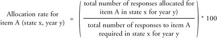
The allocation rate for United States is calculated by summing over the total number of responses allocated and responses required for an item across all states. The overall item allocation rate for the questions determining ELL status for 20052008 is from the Census Bureau.14
As shown in Table 2-13, the number of responses allocated or imputed re-
|
13 |
From the Census Bureau, see http://www.census.gov/acs/www/UseData/sse/ita/ita_def.htm [May 2010]. |
|
14 |
The item allocation rates for 2005 are for housing units only; the item allocation rates for 2006 to 2008 include housing units and group quarters populations. |
sponses for “Speaks another language at home,” “Language spoken,” and “English ability” items are very low.
We note that the amount of imputation over the period from 2005 to 2007 for all items has increased, which relates to the issue of response rate to surveys in general. The amount of imputation is also of concern because it introduces a variability that is not currently factored into the estimates of sampling errors from the ACS (National Research Council, 2007, p. 254).
CONCLUSION 2-5 Item nonresponse is a troublesome and growing issue for items used in the calculation of the number of English language learner children and youth.


