
D
Variability in Month-to-Month Changes in the Seasonally Adjusted Merchandise Trade Balances
The data on the seasonally adjusted trade balance typically fluctuate widely from month to month, as has been noted in the body of this report. Evidence shows that many users of these data, including traders and other participants in financial markets in the United States and elsewhere, sometimes overreact to monthly changes in the data. Such overreaction is sometimes attributed to ignorance concerning the extent of the underlying variability in the month-to-month changes, which can lead to misinterpreting a given month's observation as a large deviation and hence indicative of a shift in trend when it is within a range or band that could be considered reasonable in the light of the history of variability in the data.
But this phenomenon raises the key question: How should the variability in the data be measured? This appendix explores the issue of variability in the month-to-month changes in the seasonally adjusted trade balance, develops a measure of this variability that takes account of the autocorrelation that is present in the data series, and uses this measure to determine a band for the monthly changes from February 1987 through February 1991, thus providing a simple characterization of the variability in the data. Several other features of the data extending back to 1977 are also considered.
This appendix was prepared by panel member W. Allen Spivey.
Figure D-1 displays the seasonally adjusted trade balance (which we denote ATB) from January 1987 through February 1991, and Figure D-2 shows a plot of the month-to-month changes (or first differences, denoted DATB) in the ATB series from February 1987 through February 1991. The DATB series in Figure D-2 displays considerable variability and also shows that the month-to-month changes have a pronounced alternating pattern. If the monthly change is a large and positive number for a given month t, for example, the change for the following month, t+1, tends to be smaller and is often a negative number. Conversely, if the observation for month t is a negative number, the following month's observation tends to be a positive number. Data for the ATB and DATB time series are shown in Table D-1.
PROBLEMS WITH THE DATA
One of the most difficult problems with the monthly trade data is that the seasonally adjusted balance (the difference between the value of merchandise exports and imports) for a given month does not necessarily reflect trade flows in the month: this is called the carryover problem. This problem arises when, for a variety of reasons (see Chapter 4), the data on export or import transactions for a given month include transactions that actually occurred in one or more previous months, so that the value actually reported for a given month can be much larger or smaller than it should be. For example, for several years in the mid-1980s, carryovers for imports were often as high as 50 percent of the reported monthly total and as high as 13 percent for exports, and data for a month sometimes included carryovers from as many as 18 prior months.
These carryovers mean that a plot of the time series of monthly changes in the trade balance could have a large spike for a given month when a substantial portion of the figure did not represent a large change taking place in the month but rather transactions attributable to underreporting in one or more previous months. They also mean that not only is the observation for the given month incorrectly reported, but also that those for one or more prior periods were understated and thus inaccurate. Figure D-3 shows the first differences of the seasonally adjusted trade balance data for the period January 1977 through March 1990, unadjusted for carryovers. Large spikes are shown for various months, particularly July and August of 1984 and September and October of 1985, although the monthly changes between these pairs of months are comparatively small.
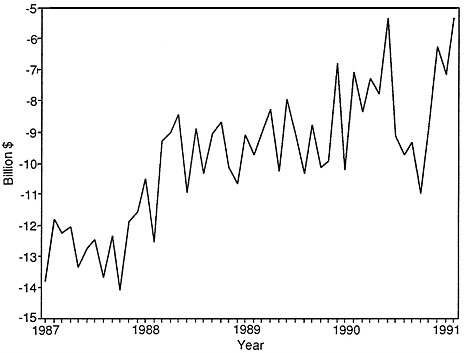
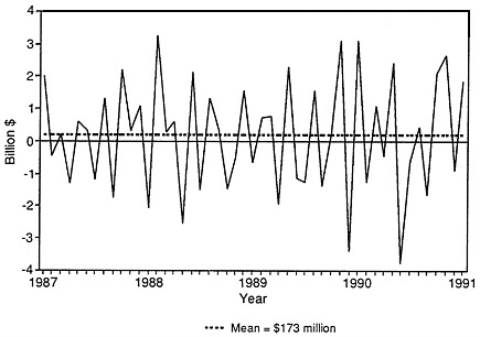
TABLE D-1 Seasonally Adjusted Trade Balance (ATB) and First Differences (DATB), 1987-1991 (in millions of dollars)
|
Year and Month |
ATB |
DATB |
|
1987 |
||
|
1 |
−13,810.2 |
— |
|
2 |
−11,813.8 |
1,996.4 |
|
3 |
−12,264.8 |
−451.0 |
|
4 |
−12,055.4 |
209.4 |
|
5 |
−13,370.3 |
−1,314.9 |
|
6 |
−12,759.6 |
610.7 |
|
7 |
−12,451.2 |
308.4 |
|
8 |
−13,659.9 |
−1,208.7 |
|
9 |
−12,345.3 |
1,314.6 |
|
10 |
−14,116.6 |
−1,771.3 |
|
11 |
−11,890.6 |
2,226.0 |
|
12 |
−11,570.4 |
320.2 |
|
1988 |
||
|
1 |
−10,495.6 |
1,074.8 |
|
2 |
−12,555.6 |
−2,060.0 |
|
3 |
−9,300.7 |
3,254.9 |
|
4 |
−9,027.4 |
273.3 |
|
5 |
−8,414.8 |
612.6 |
|
6 |
−10,969.0 |
−2,554.2 |
|
7 |
−8,859.6 |
2,109.4 |
|
8 |
−10,365.4 |
−1,505.8 |
|
9 |
−9,042.6 |
1,322.8 |
|
10 |
−8,682.4 |
360.2 |
|
11 |
−10,157.2 |
−1,474.8 |
|
12 |
−10,655.4 |
−498.2 |
|
1989 |
||
|
1 |
−9,085.2 |
1,570.2 |
|
2 |
−9,750.8 |
−665.6 |
By early 1988 carryovers had been reduced to about 5 percent for both exports and imports, and efforts to reduce carryover problems have been continuing. Unfortunately, it is not possible for the Census Bureau to make adjustments for carryover errors in the data prior to January 1987. The data in Figure D-1 and Figure D-2 and in Table D-1, however, have been adjusted by Census Bureau personnel for carryover problems. Some carryovers still exist in these data, but Census personnel believe that they do not exceed 5 percent for either exports or imports in this period.
Our analysis and measurement of the variability of the DATB time series is therefore based on the 49 observations for February 1987 to February 1991 (see Table B-1)—a relatively small number of observations that restrict the choice of methods and models available for modeling and measuring data variability.
Largely because of this small number we have used autoregressive, integrated, moving-average models, often referred to as ARIMA models, to model the autocorrelation in the DATB time series and to measure data variability. We also experimented with mod-
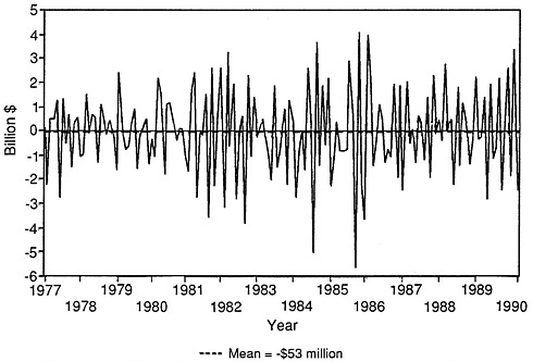
FIGURE D-3 Seasonally adjusted merchandise trade balance, first differences not adjusted for carryovers: January 1977-March 1990.
els from several other model classes, including ARCH (autoregressive conditional heteroskedastic), GARCH (generalized ARCH), and spectral models, but results were inconclusive, primarily because of the small sample size.
MEASURING THE VARIABILITY OF MONTH-TO-MONTH CHANGES
We applied the usual ARIMA modeling procedures (see Box and Jenkins, 1976: Chapters 6-8 ). Figure D-1 suggests that the levels of the seasonally adjusted trade data are nonstationary; however, the month-to-month changes or first differences DATB appear to be stationary (see Figure D-2) so ARIMA methods can be applied to them. Moreover, a perusal of discussions of the U.S. trade deficits appearing in the business media strongly suggests that data users appear to be much more interested in the month-to-month changes than in the levels of the trade deficit. 1
|
1 |
A similar situation exists with other major economic variables. Data users typically are more concerned about monthly changes in employment and in unemployment rates than with levels; changes in GNP often command greater interest than its levels, particularly when it is believed that the economy may be approaching a turning point; and money and capital markets typically direct more attention to changes, and to percentage changes, in the money supply than to the levels of the money supply. |
Proceeding to the modeling of the DATB series, Figure D-4 displays plots of the sample autocorrelation (ACF) and partial autocorrelations (PACF) and related estimates for these data. The dots in the ACF and PACF plots denote approximately 2 standard errors. Figure D-4, Figure D-5, and were developed by using Version 6.03 of the SAS computer program.
One interpretation of the ACF and PACF is that the former dies down towards zero and the PACF has a spike at lag 1. This interpretation suggests that the stochastic process generating the DATB time series is an autoregressive process of order 1, or an AR(1) process. A reasonable alternative interpretation is that the ACF cuts off after lag 1 and that the PACF dies down towards zero, so that an alternative identification is that the process is a moving average of order 1, or an MA(1) process. 2 Both of these models were estimated, and the results were subjected to the usual model diagnostic procedures. Both models produced similar and satisfactory diagnostic results, but the AR(1) model was chosen because it is easier to interpret in the context of the problem being addressed. Several other ARIMA models were examined, including an ARMA(1,1) in the first differences, but one or more coefficients were insignificant, and model diagnostics were poor.
Figure D-5 shows properties of the estimated or fitted model. The fitted model is
ŷt = − 0.56076yt−1,
where for any t, yt denotes the first difference or the change in the seasonally adjusted trade balance from time t−1 to time t. The model is estimated by means of a nonlinear maximum likelihood
|
2 |
A finite, stationary AR process can be expressed as an infinite-order MA process and a finite, invertible MA process can be expressed as an infinite-order AR process. A stationary AR(1) process, when expressed as an infinite-order MA process, can have an autocorrelation with a large spike or value at lag 1 and have a sequence of small spikes for longer lags (the autocorrelations at longer lags can be buried in the noise of the process). A similar result can occur when an MA(1) process can be expressed as an infinite–order AR process. Moreover, in applied ARIMA modeling it is not unusual to encounter a time series that can be reasonably interpreted as being generated by either and AR(1) process or an MA(1) process—as is the case here. |
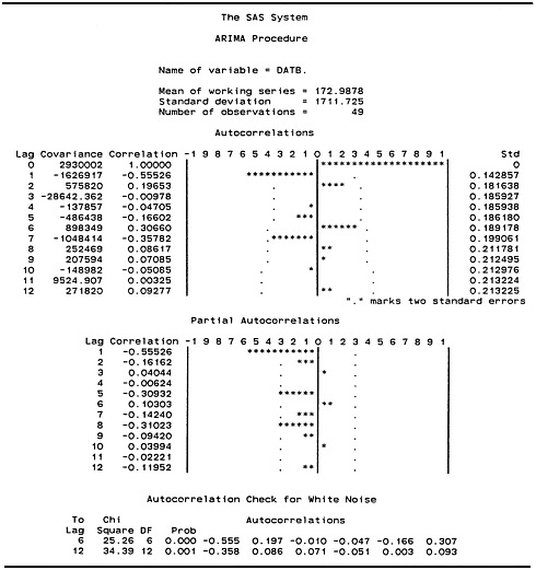
FIGURE D-4 Autocorrelations and partial autocorrelations for first differences of seasonally adjusted merchandise trade balance.
procedure as indicated in the SAS output in Figure D-5. The autocorrelation coefficient is significant at the conventional levels. The negative autocorrelation estimate, φ̂1 = −0.56076, suggests that the process generating the time series tends to produce observations that alternate in sign. Thus, one would expect a large and positive observation in a given period to be followed in the next period by an observation having a negative value.
An analysis of the residuals of the fitted model was performed.
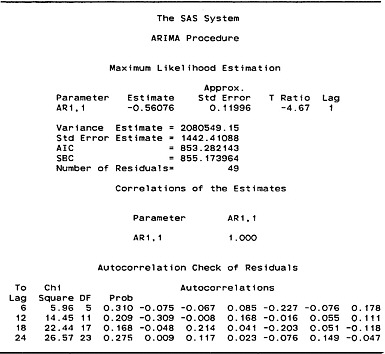
FIGURE D-5 Properties of maximum likelihood estimated model for seasonally adjusted merchandise trade data.
The autocorrelations and partial autocorrelations of the residuals (see Figure D-6) support the view that the residuals are from a white-noise process, with the possible exception of lag 7—which might indicate some residual seasonality at this lag. Joint or “portmanteau” tests for 6, 12, 18, and 24 lags (see Figure D-5) also suggest white noise (the portmanteau test is discussed in Ljung and Box [1978]). Further analysis of model residuals using a Kolmogorov-Smirnov test, a test of skewness and of kurtosis, and a p-plot of the residuals against a normal distribution all supported the adequacy of the AR(1) model.
Figure D-5 indicates that the standard error of the AR(1) model is $1.442 billion (rounded). The mean of the residuals is $249.049 million (rounded). Thus, the standard error of the month-to-month changes in the seasonally adjusted trade balance is approximately six times larger than the mean. The parameters of the AR(1) model are estimated by the SAS program using a nonlinear maximum likelihood procedure. The mean of the residuals is not necessarily zero because the sum of the model residuals is not
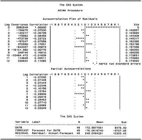
FIGURE D-6 Autocorrelations and partial autocorrelations of residuals (see Figure D-5).
constrained by the estimation to be zero, as is the case when an AR(1) model is estimated by an ordinary least-squares (OLS) algorithm. Estimation of an AR(1) model by OLS produces biased parameter estimates in finite samples. (The statistical properties of ARIMA model estimates under various nonlinear estimation procedures are examined extensively in Box and Jenkins [1976]).
The standard error of the AR(1) model estimated by SAS and used here provides an estimate of the standard deviation of the conditional distribution of yt for time t. This is an appropriate estimator to use for the standard deviation of the process generat-
ing the month-to-month changes and so is used to measure the variability of these changes.
A SIMPLE CHARACTERIZATION OF VARIABILITY
We now use the values of the mean and standard error of the residuals to develop a control chart display for the monthly changes in the seasonally adjusted trade balance data. Figure D-7 shows the first differences DATB, with a zero line, a dashed line denoting the mean of 249.0494291, and dashed lines plotted at 3 standard errors (3 × 1442.41088 = 4327.23264) above and below the mean, which can be interpreted as upper and lower control or specification limits, respectively. In other words, this is a control chart for the observations yt on the month-to-month changes. In quality-control applications, a process is typically regarded as being “out of control” when an observation exceeds a control limit, when there are aberrant sequences of observations or “runs” above and below a given level, or when a “run up” of observations alter-
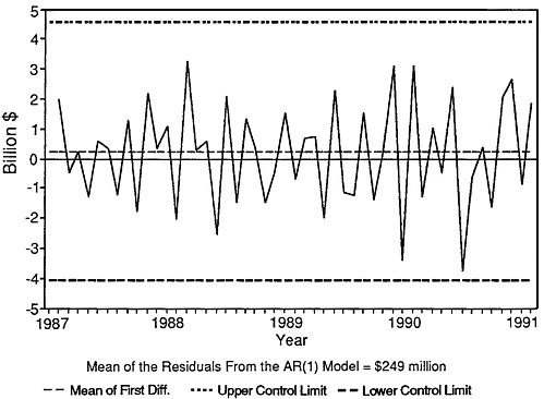
FIGURE D-7 Control chart for data on monthly changes, seasonally adjusted merchandise trade balance.
nates with a “run down” (Alwan and Roberts, 1988:87). When one or more of these conditions is displayed, one takes action in some operational sense to respond to the process.
Figure D-7 does not show an observation exceeding the specification limits, nor does it display runs. Thus, if one were to have used this approach from control charts for the period from February 1987 through February 1991, one would not have taken action because of extreme values or aberrant observations at any time. Stated another way, none of the monthly changes over this period would have been regarded as sufficiently unusual to lead one to believe that the process generating the data had shifted its mean or changed in any other important way.
To sum up: the key issue here, as noted at the beginning of this appendix, is the large variability in the month-to-month changes in merchandise trade balance data. Such variability is measured by the standard error, which is about six times larger than the mean for the data. A conventional 3-standard error band is very wide and is probably much wider than would be expected on an intuitive basis by many data users. Therefore, the month-to-month changes are not outside expectations for the characteristics of the data.


