
E
An Alternative Seasonal Adjustment Procedure for Merchandise Trade Data
Some experts claim that the high volatility of the U.S. monthly trade balance is due to the fact that the trade balance, which is usually close to zero, is derived from the difference of two large figures, imports and exports. However, our analysis shows that the data do not support this claim. For example, the mean monthly merchandise trade balance for 1985-1990 is about −$10.5 billion, the mean monthly export figure for the period is $23.5 billion, and the mean monthly import figure is $34.0 billion: the difference is a substantial proportion of the means.
We have considered alternative methods of seasonally adjusting the data because all initial analysis of the data leads us to believe that the X-11 seasonal adjustment procedure currently used by Census Bureau not only fails to remove much of the seasonal noise from the data, but also adds more noise to the data.1 Figure E-1 shows that the seasonally unadjusted series has a clear seasonal pattern. The X-11 adjusted trade balance, shown in Figure E-2, displays only slightly less volatility than the original series, and a seasonal pattern is still discernible. The standard deviation
This appendix was prepared by panel member Jerry A. Hausman; Mark Watson, professor, Northwestern University; and Ruth Judson, a graduate student at the Massachusetts Institute of Technology.
|
1 |
In this paper we concentrate on the customs valuation of imports; however, use of c.i.f. value of imports leads to very similar conclusions. |
of the unadjusted series over the 1985-1990 period is $2.1 billion, and the standard deviation of the adjusted series is $1.9 billion.
We propose an alternative method of seasonal adjustment that uses a time-series model with unobserved components—the Kalman filter model. We assume that each seasonally unadjusted trade balance figure is actually the sum of three components that are not observed individually: a nonseasonal term, representing the component of trade that varies due to economic conditions unrelated to the time of year; a seasonal term, representing the component of trade that varies due to the season; and an error or noise term.2 This can be written as
(1) Yt = Nt + St + et.
We then assume a time-series structure for each term. We model the first two terms, Nt and St, as 1-period and 12-period random walks and et as white noise to yield the following ARIMA process for the observed trade balance:
(2a) (1 − L)Nt = ent, and
(2b) (1 + L + L2 + . . . + L11)St = est.
With this model, the process is then characterized by a variance parameter for each error component. For each combination of variance parameters, the Kalman filter algorithm finds the optimal decomposition of the process into the three unobserved components given in equation (1), assuming the structure from equations (2a) and (2b). The Kalman filter also yields a likelihood value for each decomposition so that we can choose the variance components to maximize the likelihood. Once we have the optimal decomposition at the optimal variance parameter values, the model-based seasonally adjusted estimate is simply the nonseasonal component.3
The first model-based seasonally adjusted trade balance is given in Figure E-3. The graph is considerably smoother than the X-11 output. Only data available at the time t, when the trade balance was announced, were used to produce the series shown in
|
2 |
See Hausman and Watson (1985) and Hausman and Watson (1990); note that the 1985 paper uses a basic ARIMA model, and the 1990 paper allows for heterogeneity in the seasonal component. |
|
3 |
This approach is analogous to doing a regression with seasonal dummies and then defining the adjusted estimate as the data minus the fitted seasonal components from the regression. |
Figure E-3.4 The standard deviation of the model-based adjusted series is $1.5 billion, which is considerably lower than that of the X-11 series.
Figure E-4 uses historical data to seasonally adjust the data. That is, to estimate the seasonally adjusted trade balance at time t, we used data that became available after time t. This figure is probably the “best” to use for comparison with data from Census Bureau procedures since the Census Bureau uses historical data when it applies the X-11 procedure. The series shown in Figure E-4 is significantly smoother than that in Figure E-3, for which only concurrent data were used for seasonal adjustment. The standard deviation of the optimally seasonally adjusted trade balance shown in Figure E-4 is $1.4 billion. Although some improvement is evident, it is interesting to note that the method that uses only concurrent data does about 95 percent as well as the method that uses historical data.
We obtained similar results for the monthly and yearly changes in the trade balance. The standard deviation of the monthly change in the trade balance is $2.6 billion for the series adjusted with X-11; for the series adjusted with the model-based procedure, the standard deviation of the monthly change is $1.9 billion. For yearly change, the X-11 procedure yields a series with a standard deviation of $2.7 billion; the model-based procedure yields a series with a standard deviation of 2.1 billion. The standard deviation of the first difference and yearly difference fall by about $0.1 billion each when historical data are used. Thus, the standard deviation of the seasonally adjusted series from the model-based procedure is usually about 20 percent smaller than that obtained by the X-11 procedure.
An even more appropriate comparison uses the basic underlying series (nt in Hausman and Watson, 1985, 1990) after the seasonal component has been removed. The historic filter comparison is probably the most relevant since it uses the same data used by the Census Bureau to report its seasonally adjusted series. In Table E-1, we present data on three series: the monthly trade balance (Nt), the change in the monthly trade balance (Nt − N(t−1)), and the annual change in the monthly trade balance (Nt − N(t−12)). All three numbers are used in announcements and subsequent analyses. The ratios of the root mean square errors demonstrate
|
4 |
We refer to these data as concurrent data; however, the description is only approximately correct since the data are subsequently revised by the Census Bureau. We have only had access to the final revised data. |
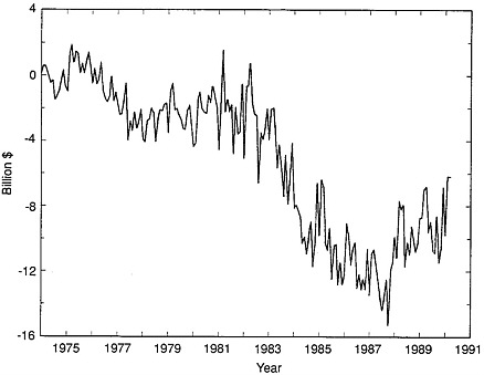
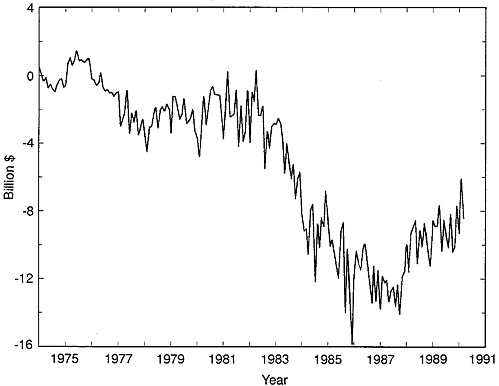
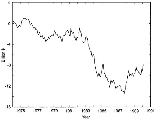

TABLE E-1 Trade Balance (Exports Minus Imports), Seasonally Adjusted Data, Root Mean Square Error (in millions of dollars)
|
A. Homoskedastic Model |
|||
|
Model |
Nt |
Nt − N(t−1) |
Nt − N(t−12) |
|
Historical Filter |
|||
|
Optimal |
351.0 |
543.7 |
240.0 |
|
X-11 |
822.9 |
1,144.4 |
1,270.6 |
|
Ratio: optimal/X-11 |
0.426 |
0.475 |
0.189 |
|
Concurrent Filter |
|||
|
Optimal |
462.9 |
709.7 |
254.0 |
|
X-11 |
895.4 |
1,153.9 |
1,275.8 |
|
Ratio: optimal/X-11 |
0.517 |
0.615 |
0.199 |
|
Comparison |
|||
|
Our concurrent |
462.9 |
709.7 |
254.0 |
|
Government historical |
822.9 |
l,144.4 |
1,270.6 |
|
Ratio: government historical/our concurrent |
0.563 |
0.620 |
0.200 |
|
B. Heteroskedastic Model |
|||
|
Model |
Nt |
Nt − N(t−1) |
Nt − N(t−12) |
|
Historical Filter |
|||
|
Optimal |
355.0 |
552.5 |
265.6 |
|
X-11 |
801.0 |
1,120.7 |
1,229.2 |
|
Ratio: optimal/X-11 |
0.443 |
0.493 |
0.216 |
|
Concurrent Filter |
|||
|
Optimal |
460.7 |
703.5 |
287.0 |
|
X-11 |
901.4 |
1,191.1 |
1,258.6 |
|
Ratio: optimal/X-11 |
0.511 |
0.591 |
0.228 |
that the optimal model-based filter does significantly better than the X-11 procedure: for the homoskedastic model-based procedure using monthly figures, the root mean square error of the model is just 0.43 as large as that for the X-11 procedure; for the monthly change figures, the model-based procedure is 0.48 as large; finally, using yearly change data, the model-based procedure is 0.19 as large. Evidently, much of the variability in the trade balance data is created by an adjustment procedure that is extremely nonoptimal.
Even if we compare the optimal seasonally adjusted series using only concurrent data with the Census Bureau series, which uses historical data, the improvement is still large. The monthly
|
C. Heteroskedastic Model, RMSE of Estimated Nt, Monthly Values |
||
|
Historical Filter |
||
|
Month |
Optimal |
X-11 |
|
January |
446.5 |
852.1 |
|
February |
335.4 |
838.3 |
|
March |
258.4 |
788.4 |
|
April |
278.1 |
775.4 |
|
May |
342.2 |
777.6 |
|
June |
324.4 |
791.2 |
|
July |
379.7 |
787.2 |
|
August |
379.7 |
808.6 |
|
September |
338.1 |
808.6 |
|
October |
338.4 |
791.6 |
|
November |
374.6 |
791.7 |
|
December |
464.3 |
801.3 |
series has a root mean square error about 0.56 as large; the monthly change ratio is 0.62 as large; and the yearly change ratio is 0.20 as large. Thus, using only data available at the time of the initial announcement of the trade balance produces a seasonally adjusted series that has considerably less variation than the Census Bureau's X-11 procedure, which uses historical data. Considerable room for improvement thus exists in the X-11 procedure used for trade balance data.
This research is suggestive of one of the serious problems with the trade balance data reported by the Census Bureau, although it cannot be taken to be definitive. We have used the revised trade data rather than the initial announcement data.5 Substantial adjustments are often made in the initially announced trade data, which is another source of variability. Hausman and Watson (1990) use a model that accounts for data revision. However, we were unable to obtain from the Census Bureau a consistent series for the unadjusted trade data, which would allow us to control for this additional source of variability. (The data were not available
|
5 |
Since government statisticians also use revised data, the comparison of the two methods is valid. |
so we could not extend our method.) A model-based procedure would permit a significant reduction in the additional variability contained in the initial announcement data since the Kalman filter model permits a forecast of the unadjusted data that would be averaged in an optimal way with the announced data. We expect that the resulting weighted average would eliminate much of the variability before the revisions are made.


