
G
Full Framework Example:
Global Land Carbon Sinks
Quantified Objective: Determine the global land carbon sink and quantify this globally to ±1.0 Pg C year−1 aggregating from the 1° × 1° scale.
IMPORTANCE
Carbon cycles through the atmosphere as gases, such as carbon dioxide (CO2) and as carbon in plants and soils, in ocean water, in phytoplankton, and in marine sediments. CO2 is released to the atmosphere from combustion of fossil fuels, by land cover changes on Earth’s surface, by biomass burning, by respiration of green plants, and by decomposition of carbon in dead vegetation and in soils, including carbon in permafrost. The atmospheric concentrations of CO2 control atmospheric temperatures, through their absorption of outgoing long wave radiation and thus indirectly control sea level, via regulation of planetary ice volumes and ocean temperatures. A depiction of the carbon cycle showing reservoirs, fluxes or transfers between reservoirs, and the processes responsible is shown in Figure G.1.
Using the atmospheric O2/N2 ratio and the change in atmospheric d13 C, an average global land carbon sink of 2.9 ±0.8 Pg C per year has been determined (Le Quéré et al., 2014). This determination is a global number with no spatial specificity of any kind. Because the land removes a quarter of the carbon emitted to the atmosphere, we need to determine the locations of and mechanisms for this large terrestrial carbon sequestration (Figure 4.1). To achieve this quantified objective, satellite observations of CO2 fluxes at monthly time-scales and spatial scales of ~1° × 1° over multiple annual cycles are critical, in addition to several other satellite observing systems. These satellite observations must be linked to process models at the 1° × 1° scale. For major urban areas, and for estimation of anthropogenic emissions, flux determinations need to be at spatial scales on the order of 10 km.
At the same time, soil respiration and decomposition must be addressed with linked of in situ process studies and satellite data sources to determine how this important land carbon cycle component can be addressed. Should the land carbon sink cease or diminish, atmospheric CO2 concentrations would increase more rapidly.
The current system of atmospheric CO2 measurements do not adequately constrain land process-based carbon cycle models to allow diagnosis and/or attribution of the land and ocean carbon sinks and sources/fluxes with any confidence—hence, the models yield widely varying patterns of carbon land and ocean sources and sinks. Testing and improving the surface and ocean parameterizations in Earth system models that calculate the surface-
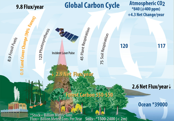
FIGURE G.1 Depiction of the carbon cycle showing reservoirs, fluxes or transfers between reservoirs, and the processes responsible. The atmospheric CO2 concentration is a principal determinant of Earth’s temperature and thus climate. Units are billion metric tons for carbon stocks and billion metric tons/year for fluxes. One ppm atmospheric CO2 is the equivalent of 2.13 Pg carbon. SOURCE: Updated from Ciais et al. (2013), with respiration data from Schlesinger and Bernhardt (2013), ocean fluxes from Westberry and Behrenfeld (2013), and land photosynthesis from Beer et al. (2010). Image courtesy of NASA Goddard Space Flight Center.
atmosphere fluxes of energy, water, and carbon, is essential for developing a capability to predict future climate, but this has proved to be a difficult and challenging task.
In addition to the required satellite observations, in situ observations are also needed to confirm satellite-measured CO2 concentrations and determine soil and vegetation carbon quantities. Understanding the carbon cycle thus requires a “full court press” of satellite and in situ observations because all of these observations must be made at the same time. The importance factor for the carbon cycle is thus assessed to be 5 as it is a fundamental component of climate and directly influences the CO2 content of the atmosphere.
UTILITY
Before the satellite era, it was impossible to quantitatively study the global regional carbon cycle. Only limited in situ measurements, such as Dave Keeling’s Mauna Loa atmospheric CO2 concentration with time, were available before the satellite era. With satellites, we are now able to quantify ocean and land photosynthesis (Westberry and Behrenfeld, 2013; Beer et al., 2010), measure the air-sea CO2 exchange (Gruber et al., 2009), measure atmospheric
CO2 concentrations (Chevallier et al., 2007), determine more accurately forest and woodland biomass (Houghton, 2005), accurately map forest disturbance and regrowth (Hansen et al. 2010), and accurately map biomass burning and determine resulting carbon emissions (van der Werf et al., 2010).
Required satellite observations to achieve accurate measurement of forest and woodland carbon involve: (1) determining the volume of carbon contained in forests and woodlands globally, a three-dimensional determination, translates into two-dimensional 30 m mapping with Landsat or equivalent, and the height or third dimension from lidar and radar; (2) disturbance mapping using Landsat or equivalent and radar at 30 m, to map deforestation and regrowth; (3) detection and quantification of biomass burning using instruments like MODIS (Moderate-Resolution Imaging Spectroradiometer) or VIIRS (Visible Infrared Imaging Radiometer Suite) that detect the thermal emissions of fires within the forest and woodland strata coupled with the biomass of the areas burned; (4) quantifying net primary production of forests and woodlands to determine the carbon uptake or release of forests; and (5) passive and active monitoring of CO2 concentrations to confirm if forest and woodland are sources or sinks of atmospheric CO2. A feature of the carbon cycle, like other quantified science objectives such as mesoscale convective system evolution, precipitation and the hydrological cycle, and surface fluxes of heat is the requirement for simultaneous observations from several satellite observing systems.
The utility rating for achieving the carbon cycle objectives of CO2 concentrations, land photosynthesis, land biomass and change, biomass burning, and respiration and decomposition is estimated to be 1.0 because of the impressive existing, new, and planned satellite systems that address carbon cycle processes directly.
QUALITY
To achieve the accuracy and precision required for quantifying the global land carbon sink ±1.0 Pg C per year by aggregation from 1° × 1° land surface data requires use of satellite data from GOSAT, OCO-2 (Orbiting Carbon Observatory-2), SMAP (Soil Moisture Active-Passive), Landsat, and MODIS/VIIRS. These satellite observing systems must be coupled to numerical land process models at the 1° × 1° scale over multiple annual cycles. The quality of quantifying the atmospheric CO2 concentration, land photosynthesis, and biomass burning is determined to be 0.95 because these components for this quantified science objective will have improved respective accuracies when surface weighted XCO2 (column-averaged CO2 concentrations) estimates are retrieved from high-resolution GOSAT and OCO-2 spectroscopic observations. The quality for land biomass and change and respiration and decomposition are both estimated to be 0.8 because of the large uncertainties in these carbon cycle components (Table 4.4). Gaps in all of these carbon cycle observations can be tolerated for periods of <1 year while continuity over spans of tens of years is needed.
SUCCESS PROBABILITY
Landsat and MODIS satellites have all operated for much longer time spans than their design lives, including 27 years for Landsat-5 and 15 years for MODIS on the Terra platform. Landsat-8, MODIS/VIIRS, GOSAT (Greenhouse gases Observing Satellite), OCO-2, and SMAP are currently operating successfully and the GEDI (Global Ecosystem Dynamics Investigation) laser altimeter mission is scheduled for launch in 2020. The probability of success for atmospheric CO2 concentration retrievals is estimated to be 0.95 because OCO-2 is operating successfully. The probability of success for land photosynthesis is estimated to be 0.9 because, while MODIS and VIIRS are operating successfully, SMAP data are needed to improve land photosynthesis and this work is just beginning. The probability of success for land biomass, disturbance, and recovery is estimated to be 0.8 because our current estimates of total above-ground plant carbon has an uncertainty of ±100 Pg C. The probability of success for biomass burning is estimated to be 0.95 based on the successful use of Landsat and MODIS/VIIRS to estimate carbon emissions from biomass burning. The probability of success for determining soil respiration and decomposition is estimated to be 0.8 because this is the largest land surface flux uncertainty (Table 4.4). While SMAP data are just beginning, the linkage of SMAP data with in situ soil respiration and decomposition process models needs to be accelerated for greater carbon cycle understanding.
TABLE G.1 Final Continuity Scoring for the Quantified Objective Global Land Carbon Sinks
| Importance | Utility | Quality | Success Probability | Benefit | |||||
| (I) | (U) | (Q) | (S) | (B) | |||||
| CO2 concentrations | 5 | 1 | 0.95 | 0.95 | 4.5 | ||||
| Land photosynthesis | 5 | 1 | 0.95 | 0.90 | 4.3 | ||||
| Land biomass and change | 5 | 1 | 0.80 | 0.8 | 3.2 | ||||
| Biomass burning | 5 | 1 | 0.95 | 0.95 | 4.5 | ||||
| Respiration and decomposition | 5 | 1 | 0.8 | 0.80 | 3.2 | ||||
FINAL SCORING
Final continuity scoring for the quantified objective is given in Table G.1 using the benefit (B) formula from Chapter 3 of B = I × U × Q × S, where I ranges from 1 to 5, U ranges from 0 to 1.0, Q ranges from 0 to 1.0, and S ranges from 0 to 1.0 (see Section 4.4 for scoring rationale).
Of the five components needed to achieve the quantified objective for land carbon sink, atmospheric CO2 measurements and biomass burning score the highest benefit score because they have the lowest measurement uncertainties. Land biomass and respiration/decomposition have the highest uncertainties and have the lowest benefit rating. Land photosynthesis falls between these carbon cycle components. All five of these components are needed to achieve the objective of identifying the land carbon sink while quantifying this globally to ±1.0 Pg C per year aggregating from the 1° × 1° scale.
REFERENCES
Beer, C., M. Reichstein, E. Tomelleri, P. Ciais, M. Jung, N. Carvalhais, C. Rödenbeck, et al. 2010. Terrestrial gross carbon dioxide uptake: Global distribution and covariation with climate. Science 329:834-838.
Chevallier, F., F.-M. Bréon, and P.J. Rayner. 2007. Contribution of the Orbiting Carbon Observatory to the estimation of CO2 sources and sinks: Theoretical study in a variational data assimilation framework. Journal of Geophysical Research 112: D09307.
Ciais, P., C. Sabine, G. Bala, L. Bopp, V. Brovkin, J. Canadell, A. Chhabra, et al. 2013. Carbon and Other Biogeochemical Cycles. Chapter 6 in Climate Change 2013: The Physical Science Basis. Contribution of Working Group I to the Fifth Assessment Report of the Intergovernmental Panel on Climate Change (Stocker, T.F., D. Qin, G.-K. Plattner, M. Tignor, S.K. Allen, J. Boschung, A. Nauels, Y. Xia, V. Bex, and P.M. Midgley, eds.). Cambridge University Press, Cambridge, U.K., and New York, N.Y.
Dlugokencky, E., and P. Tans 2015. “Trends in Atmospheric Carbon Dioxide.” National Oceanic and Atmospheric Administration, Earth System Research Laboratory. http://www.ersl.noss.gov/gmd/ccgg/trends. Last access May 15, 2015.
Gruber, N., M. Gloor, S.E.M. Fletcher, S.C. Doney, S. Dutkiewicz, M.J. Follows, M.N. Gerber, et al. 2009. Oceanic sources, sinks, and transport of atmospheric CO2. GlobalBiogeochemical Cycles 23:GB1005.
Hansen, M.C., S.V. Stehman, and P.V. Potapov. 2010. Quantification of global gross forest cover loss. Proceedings of the National Academy of Sciences 107(19):8650-8655.
Houghton, R.A. 2005. Above ground forest biomass and the global carbon balance. Global Change Biology 11(6):945-958.
Le Quéré, C., R. Moriarty, R.M. Andrew, G.P. Peters, P. Ciais, P. Friedlingstein, et al. 2014. Global carbon budget 2014. Earth System Science Data Discussions 6:1-90.
Schlesinger, W.H., and E.S. Bernhardt. 2013. The Global Carbon Cycle. Chapter 11 in Biogeochemistry: An Analysis of Global Change (W.H. Schlesinger, ed.). Academic Press.
van der Werf, G.R., J.T. Randerson, L. Giglio, G.J. Collatz, M. Mu, P.S. Kasibhatla, D.C. Morton, R.S. DeFries, Y. Jin, and T.T. van Leeuwen. 2010. Global fire emissions and the contribution of deforestation, savanna, forest, agricultural, and peat fires 1997-2009. Atmospheric Chemistry and Physics 10:11707-11735.
Westberry, T.K., and M.J. Behrenfeld. 2013. Oceanic net primary production. Pp. 205-230 in Biophysical Applications of Satellite Remote Sensing (J.M. Hanes, ed.).


