
6
India: Population Pressure, Technology, Infrastructure, Capital Formation, and Rural Incomes
Robert E. Evenson
The real income consequences of population growth have long been a matter of policy concern. Malthus and Ricardo provided the classical analysis, showing that as populations grow relative to resources (including land, public infrastructure, and private and publicly held reproducible capital), downward pressure on labor incomes will result. A similar upward pressure on land rents would also take place. Because population growth increases with income, any set of conditions that produced an increase in real incomes would be followed by a rise in population growth, setting in motion forces bringing real labor incomes and population growth back to a subsistence equilibrium.1
This "dismal" prediction has been much modified in modern analysis. Modern analysts recognize that while a rise in incomes will lead to an increase in population growth, the associated rise in the price of (labor) time will generally induce a decrease in family size and population growth. This is because the "costs" of producing relatively ''time-intensive" goods, such as children, typically rise more rapidly than does income. In addition, the income effect on child quality may dominate the income effect on child quantity, and this will also induce smaller family sizes.2 Thus, escape from the Malthusian "trap" is possible.
Four investment activities are today deemed to be critical to generating the rising real income necessary to escape from the Malthusian trap. These are investments in: (1) public sector infrastructure, (2) publicly and privately held reproducible capital, (3) human capital, and (4) research to produce improved technology. There is ample historical evidence that these investments produce growth. Every modern developed economy can account for most of its real per capita economic growth in terms of these activities.3
A controversy remains, however, as to the effect of population growth in the presence of these activities. This is because it is alleged (a) that population growth itself induces some of the investments in growth-producing activities (Boserup), and (b) that large populations may actively enhance the effectiveness of some of the growth-producing activities via special types of scale economics (Verdoorn, Simon).4 The modern literature on the "economic consequences of birth aversion" thus remains somewhat inconclusive as to whether these inducement and enhancement effects are sufficient to outweigh the fundamental classical, or Malthusian, effects.5
The real income consequences of improved technology are also subject to some debate. There is little doubt that technology, which enables more output per unit of input, increases aggregate income. However, because technology, especially agricultural technology, has a regional, or location-specific, dimension, the actual realization of these income gains between producers, consumers, and factors (i.e., labor, land) in different locations is unclear. It is quite possible that the introduction of improved technology will bring about economic losses for some groups.6
Because infrastructure and capital formation also have a regional or locational dimension, the growth in income that they produce will also have a complex distributional outcome. Furthermore, because population growth (pressure) also has a regional and locational dimension and because it has possible investment inducement and enhancement effects, population growth will interact with these activities in its effects on real income.
This paper reports an attempt to measure some of the real income impacts of population pressure, infrastructure, capital formation, and new technology in India. The first section of the chapter develops the analytic framework. The second section develops an empirical specification for testing the implications of this model and reports estimates. The third section discusses
the policy relevance of the findings. Appendix A provides an analytic model of population and technology impacts on earnings.
ANALYTIC ISSUES
A Simple One-Region Model
Consider the simplest possible case, in which only one product is produced and consumed. The market for the product is depicted in Figure 1.
The supply curve S0 is determined by profit maximizing behavior of farmers for a given level of human capital skills, infrastructure, and technology. The curve shows how supply changes as prices change. An increase in technology, human capital, or infrastructure will shift the supply curve to the right, i.e., from S0 to S1. An increase in the number of laborers will also cause a rightward shift in the supply of the product because wages will fall. This, in turn, reduces the marginal cost and producers will produce a given quantity of output at a lower price.
The demand curve is derived from the utility-maximizing behavior of consumers for given tastes and for a given population. A shift (i.e., an increase) in population will shift the demand curve to the right. Figure 1 illustrates an important point regarding the impact of a technology-induced shift in the supply curve. The shift from S0 to S1 results in a fall in the equilibrium price from P0 to P1 and an increase in output from Y0 to Y1. The decline in price results in gains to consumers (measured by the area
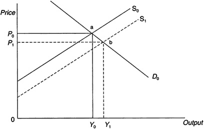
Figure 1 One-region model. D=demand, P=equilibrium price, S=supply, and Y = output.
P0abP1), and this decline is larger the more "inelastic" (with respect to price) is demand.
Revenue to the producer will change from the area P0 • Y0 (0P0aY0) to the area P1 • Y1 (0P1bY1), and this will be distributed between labor (N) and capital (K) according to the supply conditions for these factors (see below). Note that if demand is elastic with respect to price, that is, η = (dY/dP)(P/Y) is less than-1, revenue to producers will rise. If it is inelastic, revenue will fall.
Appendix A develops a mathematical model for this simple case. The features of the model are:
-
shifter variables for population, technology, labor supply and capital supply are incorporated into the model;
-
an equation showing how equilibrium prices of labor and capital are affected by these shifters is derived;
-
the analysis shows that the growth rate of the equilibrium wage rate, a key variable for income analysis because low-income families earn the bulk of their income from wages, is affected in the following ways by the shifters:
-
An increase in technology (or infrastructure) has a positive impact on (nominal) wages if demand is elastic. This is because total revenues increase when demand is elastic, as they do when the good is internationally traded. When demand is inelastic the growth in nominal wages will be lower, but the growth in real wages when technology increases is generally positive because the price of the product falls.
-
The effect on wages of an increase in the capital stock (i.e., a shift in the supply of capital) will depend on the ease with which capital can be substituted for labor. If it is relatively easy to substitute the more abundant capital for labor, nominal wages will be reduced. The effect also depends on the elasticity of demand. The more elastic is demand, the more likely it is that increased capital will aid labor.
-
The effect of an increase in population can be considered in two parts. The size of the labor force increases along with the population. An increase in the number of workers has a negative effect on wages. Population growth, on the other hand, increases demand, and this has a positive effect on wages. The combined impact depends on the ease of substituting labor for capital and on the elasticity of demand. In an economy in which there is little or no capital (a classical Malthusian economy), the effect of population growth on wages is negative. If the economy is capitalized and labor can be easily substituted for capital, population growth can lead to higher nominal (and real) wages.
-
When the capital stock grows at the same rate as the labor force and population, wages do not change.
-
An Extension to Two Regions
These results are derived under the supposition that all producers have equal access to technology. Many studies have shown that agricultural technology is quite location specific, so that technology suited to one region is not actually available for another.
It is simple to extend Figure 1 to a two-region case to obtain a basic insight about regionalization (see Figure 2).
Because suppliers are competitive, the supply curves can be added up for any price. Suppose in the two regions, 1 and 2, S10 is the supply curve for region 1 producers. The total supply curve for both regions is S10 + S20. The initial market equilibrium is at P0, with Y10 produced in region 1 and Y20 in region 2.
Now suppose technical change shifts the supply function for region 2, but not region 1. Most new agricultural technology is location specific and some regions are advantaged, others disadvantaged. The equilibrium price falls to P1, and region 1 producers now produce less (Y10 − Y11). Region 2 producers will produce more Y21 − Y20 and they produce more under all demand conditions.
Thus it is clear that producers in region 1 will lose revenue as a result of technology introduced in region 2 unless demand is perfectly elastic. Returns to fixed factors in region 1 will decline (by P0ac P1) if labor is perfectly mobile, that is, if it moves freely from one region to another, It is,
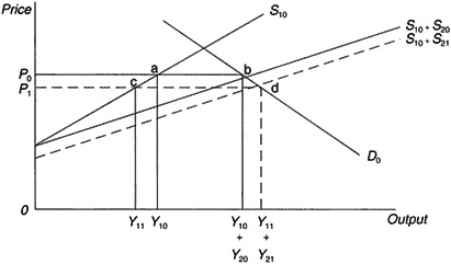
Figure 2 Two-region model. D = demand, P = price, S = supply, and Y = output.
of course, possible that labor markets may be segmented, i.e., that labor will not move easily from region 1 to 2.
One can intuitively see that if labor is not mobile, region 1 will suffer a wage decline (and this will affect S10, shifting it rightward, partially restoring the production and employment effect). Returns to fixed factors will also fall in region 1, but not as much as they would if the labor markets were not segmented. Conversely, in region 2 a segmented labor market will permit a wage rise, shifting S21 upward and modifying the gains to fixed factors as well as to output and employment.
However, if labor is mobile, wages will be the same in both regions. Wages will thus fall less in region 1 and rise less in region 2 than they would in a segmented market (the actual change will be governed by the [η + 1] condition [see equation 10 in Appendix A]). This will accentuate the loss to fixed factors in region 1 and the gain to fixed factors in region 2.
It is important to note that in a segmented labor market, labor in the disadvantaged region will be harmed by technological gains in the advantaged region as long as demand is not perfectly elastic. However, when labor is mobile it may gain from technical change in the advantaged region as long as demand is elastic. Labor in the advantaged region will gain from its own technology as long as its demand is elastic. This gain will depend on the mobility of labor.
This same logic applies to differential population growth in a region. Slower population and labor force growth have the same effect as more rapid technology growth.
An Extension to Three Regions
The two-region model can be easily extended to a three-region model. Figure 3 depicts such a model. It shows a supply shift in region 2. This shift with no labor mobility will reduce the demand for labor in regions 1 and 3 and increase demand in region 2. With mobility, labor will move from (1) to (2) and from (3) to (2), shifting the technology effect to land or fixed-factor rents.
This three-region perspective is useful in terms of analyzing limited mobility as well. Suppose that labor moves easily from (1) to (2) but not from (1) to (3). Then technical change in (2) could have a positive impact on wages in (1) whereas technical change in (3) would have a negative effect on wages in (1). Accordingly, distance and other barriers to migration are important factors to consider in assessing technical change and population effects for advantaged and disadvantaged regions.
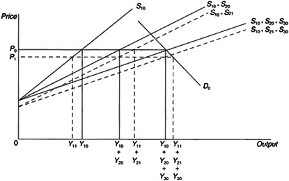
Figure 3 Three-region model. D = demand, P = price, S = supply, and Y = output.
EMPIRICAL TESTS: AN APPLICATION TO INDIA
Two empirical strategies for testing the impact of population growth on real income are available. The first is the construction of a ''general equilibrium" model in which product markets and factor markets are modeled from econometrically estimated supply and demand functions. Population, technology, and infrastructure variables can then be included in these equation estimates. Given a properly estimated model, simulations can be carried out in which population, technology, and infrastructure change impacts on equilibrium prices and quantities can be estimated (or simulated). From these estimated changes in prices and quantities, real-income effects on particular groups (e.g., landless households or small farmers) can be simulated (see Evenson, 1991).
The second strategy is to estimate a "reduced-form" specification of determinants of real wages and rental income in agriculture. Technology, population, and infrastructure variables can be included in this analysis. This strategy is somewhat more amenable to estimating enhancement and inducement effects of population pressure and it also enables much simpler measurement of regional technology effects. The second strategy is pursued here for rural India for the 1959–1984 period.
The strategy used in this study is undertaken in two stages. In the first stage an induced investment analysis is undertaken in which lagged popula-
tion density variables are treated as predictors of investment in agricultural research, agricultural extension, rural roads, rural markets, and changes in net irrigated area and net cropped areas. This analysis shows that while a considerable amount of investment could be treated as being induced by population change, much of this investment was the result of strategic planning. Accordingly, it was not deemed appropriate to predict investment from the Stage I equation for use in the second stage, but rather to utilize these estimates as auxiliary estimates of induced effects.
The second stage then entailed an analysis of real returns to labor and to land for farmers and laborers in India. The determining variables were population growth, technology flows—both domestically produced and imported—and infrastructure. These variables were specified as "stock" variables (in contrast to the investment variables in Stage I). Population density variables are interacted with these variables to estimate population enhancement effects.
Variable Definitions and Means—Stage I
Table 1 summarizes the Stage I variables.7 The dependent variables are annual investment in research and extension (technology), rural markets and roads (infrastructure), irrigation, and new cropped area. Each of these variables is treated as jointly determined by the full set of exogenous determining variables.
The determining variables are lagged stock variables. The population density, or "pressure," variable is computed as the 1956 state rural population divided by the 1984 net cropped area. Note that this is not a population growth variable. The 1984 net cropped area is treated as a better measure of potential cultivable land than is the 1956 level of net cropped area. This variable is computed for the state rather than the district to achieve more "exogeneity." (The dependent variables are district-level variables, although for research and extension these are effectively state-level variables.) The actual estimates included a number of interaction variables (discussed below).
Variable Definitions and Means—Stage II
Table 2 reports similar variable definitions for the second-stage analysis. The endogenous dependent variables are the index of real wages paid to rural workers and the index of estimated market rents for land. Note that both are measured at the district level and all are indexed on 1956–1959
TABLE 1 Variable Definitions and Means: Stage I Analysis
|
Variable |
Definition |
Mean |
SD |
|
1. Endogenous (dependent) |
|||
|
RESEXP |
Annual real expenditures on research in the state |
252 |
324 |
|
EXT |
Annual man-days of extension per district |
3.79 |
3.93 |
|
IMKTS |
Number of markets in the district, indexed to 1956 = 1 |
2.30 |
2.62 |
|
INROADL |
Road length per net cropped area in 1984 in district, indexed to 1956 = 1 |
1.744 |
1.927 |
|
INIA |
Net irrigated area in district, indexed to 1956 = 1 |
2.160 |
2.296 |
|
INCA |
Net cropped area in district, indexed to 1956 = 1 |
1.064 |
0.142 |
|
II. Exogenous (independent) |
|||
|
MSPDEN |
State population in 1956 net cropped area in 1984 |
3006 |
1843 |
|
LITERACY |
Percentage of rural males who are literate |
0.307 |
0.104 |
|
IADP |
Dummy = 1 for intensive agriculture district |
0.035 |
0.182 |
|
MNCA |
State mean net cropped area per district (000 ha) |
477 |
272 |
|
MNIA |
State mean net irrigated area per district (000 ha) |
70 |
77 |
|
WHYV |
Percentage of cereals planted in high-yielding varieties |
0.124 |
0.183 |
|
ISOUT-IN |
Index of state total factor productivity gains (1956 = 1) |
1.22 |
0.27 |
|
INOUT-IN |
Index of geoclimatic neighbor total factor productivity gains (1956 = 1) |
1.25 |
0.23 |
|
IFOUT-IN |
Index of other district total factor productivity gains |
1.27 |
0.22 |
|
AGRO |
Agroclimatic region dummies |
— |
|
|
YEAR |
Time (1956–1987) |
— |
|
|
YEAR2 |
YEAR squared |
— |
|
values. Thus in the reduced form model underlying these variables, the 1956–1959 differences between districts are treated as predetermined by a number of social and economic factors (including population density) prior to the postindependence period. Changes in these returns to labor and land over the 1956–1959 to 1983–1984 period are thus the object of analysis.
The determining variables are population, technology, and infrastructure variables. Population is modeled as having an "enhancement" effect and a growth effect. Two population variables are constructed, both at the state level (to avoid endogeneity as much as possible). The MSPDEN variable is a population pressure variable and it is treated as the enhancing variable (in interaction with other variables). The ISPDEN variable is a growth variable indexed as being equal to one during 1956–1959 at the state level. Thus, population growth is treated as exogenous to the district on the grounds that it is determined primarily by other dependent variables in the analysis as well as by the natural process of population growth. It is treated as an inducing variable.
TABLE 2 Variable Definitions and Means: Stage II Analysis
|
|
|
Means |
|
|
Variable |
Definition |
All India |
N. India |
|
1. Endogenous (dependent) |
|||
|
IRWAGE |
Rural wages paid to male laborers, deflated by worker CPI, indexed to 1956 = 1 |
1.017 |
1.100 |
|
IPNCA |
Reported land rent per ha Net cropped area deflated by CPI, indexed to 1956 = 1 |
2.614 |
2.372 |
|
II. Exogenous (independent) |
|||
|
ISPDEN |
State rural population/net cropped area in 1984, indexed to 1956 = 1 |
1.254 |
1.252 |
|
MSPDEN |
State population in 1956, net cropped area in 1984 |
3024 |
3301 |
|
NIAI |
District ratio of net irrigated area/net cropped area |
0.238 |
0.435 |
|
MKTS |
Rural markets per district |
10.66 |
12.37 |
|
LITERACY |
Percentage of rural males literate |
0.308 |
0.294 |
|
ROADL |
District road length/net cropped area 1984 |
2001 |
1186 |
|
IADP |
Dummy = for 1 intensive agricultural district |
0.035 |
0.031 |
|
WHYV |
Percentage of cereal acreage planted in high-yielding varieties |
0.126 |
0.154 |
|
IOUT-IN |
District total factor productivity, indexed to 1956–1959 = 1 |
1.217 |
1.339 |
|
ISOUT-IN |
State of total factor productivity index, 1956–1959 = 1 |
1.212 |
1.341 |
|
INOUT-IN |
Geoclimatic neighbor district total factor productivity index, 1956–1959 = 1 |
1.247 |
1.341 |
|
IFOUT-IN |
Nonneighbor district total factor productivity index, 1956–59 = 1 |
1.276 |
1.194 |
|
YEAR |
|
|
|
The technology variables are of two types. The WHYV, which measures the proportion of area planted in high-yielding varieties, is treated as measuring one component of new technology, much of it imported from abroad. This variable is endogenous at the farm level but can be considered to be exogenous at the district level.8
The main technology variables, however, are the Divisia-based total factor productivity (TFP) indexes. These are defined for the district, for the state in which the district is located, for the districts outside the state but in the same geoclimatic region, and for all other districts. The attempt here is to measure the differential impact of technology in the district and in other regions (as discussed in Figure 3).9 Other variables measure infrastructure and capital stock variables.
Stage I Estimates
Table 3 summarizes the Stage I estimates of population-induced investment effects. The regression estimates utilized a common set of independent variables including several ''interaction" variables. The impacts shown in Table 3 are "elasticities" computed at sample means. Table B-1 in Appendix B reports the full regression estimates.
The major variable of interest is the population pressure variable, MSPDEN. These estimates show that population pressure induces significant investment in agricultural research (but not enough to offset population growth, i.e., the elasticity is less than one). Population pressure also induces some investment in agricultural extension. The interaction of the population pressure variable with the HYV (high-yielding varieties) access variable strengthens these technology inducement effects.
Population pressure has mixed impacts on infrastructure. It appears to stimulate road investments but does not stimulate the development of improved rural markets. The road-inducement effect is strengthened by HYV availability (some of these HYVs were imported from abroad).
The effect of population density on irrigation and cropped areas is negligible. The level of adult literacy appears to have relatively minor impacts on investments, except for small extension and irrigation impacts.
Past technological changes have some regional effects, but on the whole the net overall effect of past technological success on investment is minor. HYV availability does not induce significant investments. The IADP (intensive agricultural district) effects are minor (though not in the IADP districts, where they did have major impacts on markets, roads, and irrigation).
Research investment tends to respond positively to the state's own productivity record, but negatively to the production change in competing regions. This is also the case for extension investment. It appears that states do not attempt to invest to facilitate spill-in technology from outside the state except in markets and irrigation. (The geoclimatic neighbors variable
TABLE 3 Stage I Estimates: Population-and Technology-Induced Investment Elasticities
|
Determining Variable |
Research (RESEXP) |
Extension (EXT) |
Markets (IMKTS) |
Roads (IROADL) |
Irrigation (INIA) |
Cropped Area (INCA) |
|
MSPDEN |
.757 |
.151 |
-.183 |
.517 |
-.002 |
-.067 |
|
LITERACY |
-.136 |
.114 |
082 |
-.119 |
.251 |
-.031 |
|
MNCA |
-.092 |
-.138 |
.159 |
.310 |
.154 |
-.058 |
|
MNIA |
.055 |
.109 |
.009 |
-.068 |
-.324 |
-.009 |
|
WHYV |
-.111 |
-.111 |
.066 |
-.027 |
-.017 |
-.027 |
|
IADP |
-.002 |
-.002 |
.025 |
.012 |
.009 |
.001 |
|
ISOUT-IN |
.938 |
.731 |
-.195 |
.047 |
-.291 |
-.027 |
|
INOUT-IN |
.078 |
-.649 |
.223 |
-.478 |
.135 |
.042 |
|
IFOUT-IN |
-.973 |
-.603 |
-.103 |
.357 |
.388 |
.074 |
|
R2 |
.642 |
.833 |
.289 |
.323 |
.299 |
.264 |
|
F |
422 |
1,175 |
95 |
112 |
100 |
84 |
[INOUT-IN] represents the potential spill-in technology.) If all regions realize productivity gains at the same rate, the net effects of past productivity history are very small.
Proponents of the "invisible institutional hand" by which public sector investments are made in some optimizing fashion will be disappointed by these estimates. The determining variables explain only a relatively small part of actual investment. Investment in research and extension increased more rapidly than did population growth, for example.10
It is reasonable, however, to recognize that effective public investment is a proactive process entailing analysis, judgment, and political considerations. It is not a simple reactive process in which population density truly induces a substantial amount of investment. (Note, however, that this analysis did not include a population growth variable—see the next section. Accordingly, it would be improper to attempt to predict the "stocks" used in the Stage II analysis from these investment equations.)
Stage II Reduced Form, Income Determinant Estimates
The Stage II income determinant estimates are summarized in Table 4. As with Table 3, these estimates are reported as computed elasticities. Population enhancement interactions are noted. (Table B-2 in Appendix B reports actual estimates.)
Estimates are reported for all India (i.e., 10 states), and for four North India states. North India has benefited most from new HYV and other technology, and it is generally regarded to be the more progressive and development-oriented region of India (although it includes many poor districts).
The dependent variables are the real wages for rural (generally landless) daily workers (including payments in kind), indexed on 1956 = 1 in each district, and the real rental rate for land, which is also indexed on 1956 = 1. Thus, this is an analysis of changes in real labor and land incomes over the 1956–1984 period. The determining variables include two population variables, five infrastructure variables, and five technology variables.
The population variables are the density variable, MSPDEN, used in Stage I to measure induced investment effects, and IMSPDN, a growth index of rural laborers for the state. The population density variable is interacted with infrastructure and technology variables to measure enhancement effects. The growth variable measures the direct impact of population on incomes. (This could have been interacted as well but the basic notion
of enhancement is a density notion.) The growth variable is treated as exogenously determined by general population growth. Migration between states is viewed as being determined by other dependent variables including the initial density.
Two sets of elasticities are reported. The first (1) is computed from the second stage estimates. The second (2) adds the population-induced effects from the first stage estimates to these.11
Real Labor Income Effects
Consider the population effects. The labor force growth variable shows a clear negative impact on real wage incomes in all India and in North India. This is a large and significant effect (-.276 and-.333). The density enhancement effects are positive for all India and for North India (.026 and .096). The computed density-inducement effects are also positive(.112 and .033), and the combined enhancement and inducement effects (which interact positively with technology) are also significant. They do not outweigh the negative growth effects of population, however. For all India, the positive enhancement and inducement effects are half of the negative growth effect. For North India they are approximately 40 percent of the negative growth effects. This estimate is approximately the same as an earlier estimate for North India computed from a general equilibrium model for an earlier period (Evenson, 1991).
Although the population impacts on real labor incomes are roughly the same for North India and all India, the relative impacts of infrastructure and technology differ. For all India, both infrastructure and technology contribute to higher labor incomes, although technology is more important. For North India, infrastructure contributions are negligible and technology contributions are large. (These technology impacts are enhanced by population density in North India but not in all India.)
For all India the infrastructure impact of roads and labor income is important. Interestingly, irrigation impacts are relatively low. Literacy also has a small impact, as do markets. For North India these impacts are overwhelmed by technology impacts.
The technology impacts require interpretation in the context of the advantaged-disadvantaged region model (Figure 3). Availability of high-yielding varieties has a large positive impact on labor incomes in regions where it occurs.
TABLE 4 Stage II Estimates: Population, Technology, and Infrastructure Impacts on Real Rural Wages and Land Rents
For all India the regional estimates indicate that the productivity gains realized outside the state but in neighboring (in a geoclimatic sense) districts increase real labor incomes. District and state productivity gains have little effect. Productivity gains from "far neighbors" are competitive and reduce labor incomes. This suggests that labor mobility is important and that it has been sufficient to create a large region in which productivity gains can benefit laborers. Labor mobility, however, is not sufficient to eliminate the competitive effect from far neighbors. Note further that popu-
|
Land Prices |
|||||
|
Population Enhancement Effects |
Elasticity (1) |
Elasticity (2) |
|||
|
All India |
North India |
All India |
North India |
All India |
North India |
|
|
|
-0.530 |
0.843 |
|
|
|
|
|
-1.212 |
-0.292 |
-1.264 |
-0.342 |
|
- |
- |
0.051 |
0.017 |
0.042 |
0.014 |
|
+ |
+ |
0.051 |
0.017 |
0.042 |
0.014 |
|
- |
- |
-0.1048 |
-0.072 |
-0.045 |
-0.077 |
|
+ |
+ |
0.028 |
0.152 |
|
|
|
- |
- |
0.003 |
-0.095 |
|
|
|
- |
- |
0.080 |
-0.221 |
|
|
|
+ |
- |
-0.406 |
-0.035 |
|
|
|
- |
- |
0.173 |
-0.289 |
|
|
|
+ |
+ |
-0.820 |
-0.230 |
|
|
|
|
|
-0.970 |
-0.870 |
-1.02 |
-0.909 |
lation density enhances the ability of workers to gain from the productivity of nearby neighbors, i.e., by enlarging the region for mobility. Note also that population density worsens the competitive impact from far neighbors. If all regions realize the same rate of total factor productivity gains, the total effect of improved technology on labor incomes would be positive and significant. (Indeed a 1 percent total factor productivity gain more than offsets the net loss from a 1 percent growth in population.)
For North India, where technology in the form of green revolution
wheat (and rice) varieties has been more important, technology impacts are larger. The regional implications are slightly different. The nearby neighbor and far neighbor effects are similar to those for all India. The state and district estimates suggest a kind of submarket for labor. There appears to be a local effect (possibly a short-term effect for the abruptness of the green revolution) in which laborers gain from local technology (in addition to high-yielding variety technology and lose as a result of competition from other districts in the state. There is enough of an enhancement of mobility due to population to enable workers to benefit from near neighbors' productivity gains.
Land Income Effects
The estimated land income effects are generally consistent with the labor income estimates, with prior studies, and with economic logic. This is true despite very crude land price data.
For all India, the population impacts are negative on land incomes. For North India the growth impact is positive, whereas the enhancement and inducement impacts are negative. The enhancement and inducement effects are consistent with the negative effects of technology because these activities create substitutes for land and make it less scarce. Irrigation does as well. Markets and literacy appear to have complementary effects.
The differences in the population growth impact on land incomes between all India and North India may be due to differences in land scarcity and possibly to off-farm income opportunities. If land is scarce, population growth should have the Malthusian effect measured in North India.
SUMMARY
The reduced form estimates of the effects of population, infrastructure, and technology on labor and land incomes in India are consistent with theoretical expectations and with prior evidence from North India.
For population effects these estimates show that the Malthusian labor supply has negative impacts on labor incomes and that the impacts are partially but not fully offset by population inducement and enhancement effects. The direct growth effects on land incomes differ for North India and all India, but population enhancement and inducement effects are negative on land incomes. Infrastructure effects are small, although the existence of roads is important to labor income. Irrigation has only small effects.
New technology raises labor incomes and lowers land incomes, and these effects are stronger in North India. The geographic size of the labor market impacts due to regional productivity change is large, but does not cover the entire country. There is a competitive regional impact where
advantaged regional productivity growth reduces both labor (and land) incomes in disadvantaged regions (that is, regions not receiving the technology). Population density enlarges the area of the region that gains.
From a distributional perspective, these results support policy interventions to slow population growth (actually labor force growth) and international migration in all regions. More infrastructure investment is also called for.
Perhaps of most relevance is the very strong implication for technology. Improved technology raises rural labor income unless it is very unevenly produced, in which case productivity gains in advantaged regions may reduce labor incomes in disadvantaged regions. However, existing mobility appears to be sufficient to enable locally disadvantaged regions to escape this reduction, indeed to gain from nearby advantaged neighbors. On balance, improved technology is a major factor enabling rural India to escape, at least temporarily, the Malthusian population trap.
REFERENCES
Antle, S.M., and J.M. Capalbo, eds. 1998 Agricultural Productivity: Measurement and Explanation. Washington, D.C.: Resources for the Future.
Becker, G.S. 1988 Family economics and macro behavior. The American Economic Review 78:1–13.
Boserup, E. 1965 The Conditions of Agricultural Growth. Chicago: Aldine.
Denison, E. 1962 The Sources of Economic Growth in the United States and the Alternatives Before Us. New York: Committee for Economic Development.
Evenson, R.E. 1979 Technology access and factor markets in agriculture. Philippine Economic Journal. 1&2:1–16.
1991 Technology, infrastructure, output supply and factor demand in North Indian agriculture. Pp. 217–232 in R.E. Evenson and C.E. Pray, eds., Research and Productivity in Asian Agriculture. Ithaca, N.Y.: Cornell University Press.
Evenson, R.E., and J. McKinsey 1991 Research, extension, infrastructure, and productivity change in Indian agriculture. Pp. 158–184 in R.E. Evenson and C.E. Pray, eds., Research and Productivity in Asian Agriculture. Ithaca, N.Y.: Cornell University Press.
Hayami, Y., and V. Ruttan 1971 Agricultural Development: An International Perspective. Baltimore: Johns Hopkins University Press.
Jorgenson, D., F. Gollop, and B. Fraumeni 1988 Productivity and U.S. Economic Growth. Cambridge, Mass.: Harvard University Press.
Lee, R.D., W.B. Arthur, A.C. Kelley, G. Rogers, and T.N. Srinivasan, eds. 1988 Population, Food and Rural Development. Oxford: Clarendon Press.
Lipton, M., and R. Longhurst 1989 New Seeds and Poor People. Baltimore: Johns Hopkins University Press.
National Research Council 1986 Population Growth and Economic Development: Policy Questions. Committee on Population. Washington, D.C.: National Academy Press.
Simon, J. 1977 The Economics of Population Growth. Princeton, N.J.: Princeton University Press.
1981 The Ultimate Resource. Princeton, N.J.: Princeton University Press.
Verdoorn, P.J. 1951 On an empirical law governing the productivity of labor. Econometrica 19:209–210.
APPENDIX A: AN ANALYTIC MODEL OF POPULATION AND TECHNOLOGY IMPACTS ON EARNINGS
A Simple, Single-Region Model
Consider a single product (Ys) produced in a single region using labor (L) and an aggregate capital stock (K). The production function, F ( ), can be written as:
Ys = T(t)F(N,K), T* = dT(t)/dt, (1)
where T(t) is a neutral technology index governing all producers of Y. A shift in technology will cause more output per unit of input and will not cause the cost minimizing mix of N and K to change.
The demand for the product (D(Y, I), depicted as D0 in Figure 1) may be written as:
Yd = P(t)D(Y,I), P* = dP(t)/dt, (2)
where Yd is quantity demanded and P(t) is a population index.
Now consider the supply functions for N and K, g(PN) and k(PK):
N = N(t) g(PN), N* = dN(t)/dt; εN = (dg/dPN) (PN/N) (3)
and
K = K(t) k(PK), K* = dK(t)/dt; εk = (dK/dPK)PK /K). (4)
In equation 3 the supply of labor responds to the wage rate PN and to a shift variable, N*, which may be considered to be population-related labor force growth. The supply of capital has a similar policy-related shifter.
Producers will maximize profits (π) for any set of output prices and input prices:
Π = PY Y-PN N-PK K. (5)
Solving first-order conditions for Y, N, and K and substituting into equation 5 yields the maximized profits function:
Π* = π(PY,PN,PK,T*,P*,N*,K*). (6)
Note that this maximized profit function includes the four ''shift fac-
tors,'' T* (technology), P* (population), N* (also population and migration), and K* (capital and infrastructure). These shift factors also belong in the product supply and factor demand equation derived from profit-maximizing behavior via Shephards' Lemma:
∂Π*/∂PY = YS = YS (PY,PN,PK,T*,P*,N*,K*), (7)
∂Π*/∂PN = ND = ND (PY,PN,PK,T*,P*,N*,K*), (8)
∂Π*/∂PK = KD = KD (PY,PN,PK,T*,P*,N*,K*). (9)
Technology and population growth also shift the demand for N and K (see equations 8 and 9.)
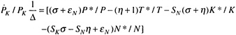
Expressions for these latter effects can be derived in this model by differentiating the system of equations 1–4 and equation 6 with respect to time and solving for the equilibrium growth rates in the price of factors. This yields:
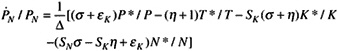
(10)
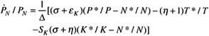
and
(11)
These expressions relate the equilibrium price paths of labor and capital (![]() and
and ![]() expressed as percentage rates of change) to changes in each of the shifter variables (P* /P, T* /T, K* /K, and N* /N, also expressed as rates of change). The additional parameters of the model are:
expressed as percentage rates of change) to changes in each of the shifter variables (P* /P, T* /T, K* /K, and N* /N, also expressed as rates of change). The additional parameters of the model are:
the factor supply elasticities, εN and εK;
the output demand elasticity, η;
the elasticity of substitution between N and K, σ;
the factor cost shares SN and SK; and
the term Δ = η(εNεK + SKεN) + εKεN + SNεN) + SKεK)−ησ. Note that Δ is positive as each term in the expression is positive.
Equation 10 is particularly important for policy analysis. It provides the basic analysis of the impacts of population and technology on returns to labor. The impact of technical change T*/T, can be seen to depend on the
elasticity of demand (as discussed in connection with Figure 1). If demand is elastic ([η + 1] is negative, hence-[η + 1] is positive), faster technical change will be associated with higher rates of change in the price of labor. These in turn will be higher the higher are σ and εK. The reverse will hold for inelastic demand. The effect of technical change on capital prices is similar. However, the distribution of gains (or losses) between labor and capital will depend on relative supply elasticities. The factor with the most inelastic supply will receive a relatively larger part of the gains. In fact, reference to Figure 1 will show that if K is strictly a fixed factor, its return will be the triangle P0 ac initially and will change to the triangle P1 bd after the new technology is introduced. These returns will not fall even when demand is inelastic.
The effect of an increase in capital, K* /K, on labor depends on the term (σ + η). If this is negative, expanding the capital stock will help labor. For example, a credit subsidy to capital will lead to a positive K* /K. If it is easy to substitute this subsidized capital for labor, i.e., if σ is high, it is more likely that labor will be harmed by this policy. If the product is traded internationally, i.e., η is large and negative, it is more likely that labor (and capital) will be helped (by the subsidy).
Equation 10 can be rewritten as equation 12 to better analyze the effects of population, P* /P, and labor force growth, N* /N:
(12)
The effect of labor force growth, N* /N, on labor earnings is negative because the second term, which depends on σ + η, cannot become positive enough as η gets large and negative because η is in Δ.
The effect of population growth, P* /P1 is positive on labor earnings. The combined effect of population and labor force growth, P* /P = N* /N, is dependent only on the σ + n term. If σ is high and η low, population growth can actually lead to rising wages. Of course, the classical economists had in mind σ = 0, so population growth had a negative impact on labor earnings. One can also see that if K* /K = N* /N = P* /P, there will be no effect on PN /PN.
It should further be noted that no inducement or enhancement effects have been considered so far. If P* /P "induced" an expansion in K* /K, this would be a positive offset in a classical world (σ = 0). If P* /P enhanced T* T, it could lead to a positive or negative effect.
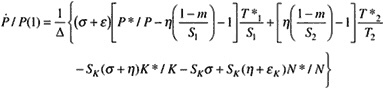
TABLE B-1 Stage 1 Regression Estimates
TABLE B-2 Stage II Real Wages and Rent Estimates, All India and North India
|
Dependent Variables |
All India |
|
|
|
North India |
|
|
|
|
|
IRWAGE |
|
RENT |
|
IRWAGE |
|
IRENT |
|
|
INTERCEPT |
5374 |
(22.58) |
-425564 |
(-2.83) |
3391 |
(4.46) |
5981 |
(1.47) |
|
IOUT-IN |
-0.018 |
(-0.63) |
-23.208 |
(-1.27) |
-0.292 |
(-1.25) |
0.754 |
(0.60) |
|
ISOUT-IN |
0.054 |
(0.86) |
114.201 |
(2.85) |
0.230 |
(0.64) |
-0.551 |
(-0.22) |
|
INOUT-IN |
0.046 |
(0.84) |
-99.825 |
(-2.86) |
-1.346 |
(-2.67) |
1.157 |
(0.43) |
|
IFOUT-IN |
0.045 |
(0.90) |
-15.475 |
(-0.48) |
0.142 |
(0.30) |
-2.921 |
(-1.16) |
|
MSFDEN |
0.000 |
(2.92) |
-0.022 |
(-2.04) |
-0.000 |
(-2.52) |
0.001 |
(1.07) |
|
IMSPDEN |
-0.225 |
(-5.43) |
5.432 |
(0.21) |
-0.293 |
(-1.12) |
3.010 |
(2.16) |
|
NIAI |
-0.505 |
(-3.76) |
-32.898 |
(-0.39) |
0.944 |
(2.66) |
2.612 |
(1.37) |
|
MKTS |
0.022 |
(6.92) |
-0.602 |
(-0.29) |
0.070 |
(4.86) |
0.342 |
(4.48) |
|
LITERACY |
-1.036 |
(-4.49) |
74.026 |
(0.51) |
-0.618 |
(-0.54) |
-4.302 |
(-0.70) |
|
ROADL |
0.000 |
(1.68) |
0.001 |
(0.14) |
-0.001 |
(-3.88) |
-0.003 |
(-3.67) |
|
IADP |
-0.054 |
(-2.90) |
0.288 |
(0.02) |
-0.074 |
(-1.65) |
-0.038 |
(-0.15) |
|
WHYV |
0.139 |
(0.75) |
113.632 |
(0.97) |
0.634 |
(0.97) |
-3.442 |
(-0.99) |
|
OUTINNIA |
0.077 |
(1.57) |
12.890 |
(0.41) |
0.638 |
(4.45) |
3.172 |
(4.13) |
|
OUTINFOP |
-0.000 |
(-1.38) |
0.004 |
(1.02) |
0.000 |
(1.81) |
-0.000 |
(-1.29) |
|
OUTINMKT |
0.007 |
(5.57) |
0.922 |
(1.15) |
0.016 |
(3.57) |
-0.030 |
(-1.26) |
|
OUTINLIT |
-0.059 |
(-0.53) |
-6.569 |
(-0.09) |
-0.519 |
(-1.40) |
-1.623 |
(-0.82) |
|
OUTINRDA |
-0.000 |
(-4.26) |
-0.007 |
(-2.38) |
-0.000 |
(-2.70) |
-0.000 |
(-1.97) |
|
NIAPOP |
0.000 |
(2.14) |
0.013 |
(1.26) |
-0.000 |
(-5.06) |
-0.001 |
(-2.97) |
|
MKISPOP |
-0.000 |
(-5.86) |
0.000 |
(0.76) |
-0.000 |
(-3.92) |
-0.000 |
(-5.72) |
|
LITPOP |
0.000 |
(0.99) |
0.017 |
(1.14) |
-0.000 |
(-1.28) |
-0.001 |
(-0.79) |
|
ROADPOP |
-5.109 |
(-0.40) |
5.730 |
(0.71) |
1.143 |
(4.20) |
8.136 |
(5.72) |
|
WHYUPOP |
0.000 |
(5.66) |
-0.028 |
(-2.46) |
0.000 |
(2.12) |
0.001 |
(2.08) |
|
WHYVNIA |
0.023 |
(0.24) |
-158.193 |
(-2.64) |
-0.062 |
(-0.21) |
-0.656 |
(-0.42) |
|
WHYMKT |
0.007 |
(2.66) |
-1.073 |
(-0.68) |
0.018 |
(1.96) |
0.154 |
(3.16) |
|
WHYVLIT |
-1.766 |
(-6.66) |
-290.020 |
(-1.73) |
-2.098 |
(-2.81) |
-12.811 |
(-3.20) |


