
Appendix C
Item Response Theory Example Using Motor Carrier Management Information System Data
Jacob Spertus
The following provides a brief worked example of an item response theory (IRT) model as discussed in Chapters 3, 4, and 5 applied to actual Safety Measurement System data. It uses a very small proportion of the full data, purposefully selected for quality and carrier size. It is not intended to be a comprehensive, unbiased analysis but merely a proof of concept. A full implementation would look roughly similar, but with many more carriers and violations included.
This appendix is included to show that the proposed model is relatively easy to implement in the Motor Carrier Management Information System. However, this model is in many ways a toy model. It is only applied to 865 carriers (not 200,000) and only unsafe driving violations that appeared for 5 or more carriers are included; there are none of the features, including multidimensionality (in fact, only one BASIC is used); and the priors have not been updated over time. Therefore, the quality of the fit should not be seen as an indication of the quality of the fit of the full model as represented in Chapters 4 and 5.
Suppose for each carrier i ∈ {1,…,C} we have a measure of exposure Ei, a count of eligible inspections nki, and a count of violations yki, where k ∈ {1,…,K} indicates the type of violation. Note that inspections are superscripted with k because the type of inspection determines which violations can be recorded. We propose the following model:
| P(Ni = ni|Ei = Poisson(λ·Ei) | (C-1) |
| P(Yik = yik | nik,pik) = Binomial(nik,pik) | (C-2) |
| logit(pik|θi) = βk + αkθi | (C-3) |
| θi ∼ N (0,1) | (C-4) |
| βk ∼ N (0,32) | (C-5) |
| αk ∼ log N (1,1) | (C-6) |
The parameter λ in equation (C-1) estimates the rate of inspections per vehicle miles traveled (VMT) across the population. pik in equation (C-2) represents the probability of carrier i receiving violation k at a given inspection. It is modeled as a logistic function of the prevalence (or difficulty) parameter βk, which reflects the marginal prevalence of violation k in the data, and discrimination parameter αk, which reflects the association of violation k and latent safety. Thus for a given violation k a higher value of βk indicates that it is observed more frequently, and a higher value of αk indicates it is more associated with safety or danger.
To implement this model on a small scale, we use SMS data from 2014 to 2015, selecting a subset of the carrier population and including only unsafe driving violations. The carrier subpopulation are those carriers with 100 or more average power units (APUs), more than 80,000 VMT per APU reported, and less than 200,000 VMT per APU reported (medium to high utilization carriers according to SMS methodology). This leaves only 865 carriers. Finally in order to set a lower bound on sparsity, we drop violations that occur in less than 5 carriers. After this processing, 35 different types of unsafe driving violations (features) remain for 865 carriers (observations).
We used the ‘rstan’ interface to Stan for Hamiltonian Monte Carlo to fit the fully Bayesian models described above (Stan Development Team 2016). In the first step, a simple Poisson model (equation (C-1) is fit. For exposure Ei, we take 100,000 VMT. λ is specified with a non-informative prior and thus gives, essentially, the average inspections per 100,000 VMT. The observed mean in the population is 2.014, while the posterior mean (95% CI) of λ is 1.806 (1.802, 1.811)
The second step uses equations (C-2) and (C-3), and priors (C-4), (C-5), and (C-6), to fit a binomial IRT model. The prior on θi is selected to enforce identifiability of the model. The log-normal prior on αk, which has support only over the positive real numbers, encodes the assumption that αk is strictly positive. We provide default choices for the priors on βk and
αk by matching the specification in the ‘edstan’ R package for IRT models (Furr, 2017). Note that substantive knowledge about the effect of certain violations on safety could be included via the prior (C-6). The ‘trials’ for this IRT model are inspections eligible for unsafe driving violations, that is, driver inspections (level 1, 2, 3, or 6). A brief caveat: unsafe driving violations (e.g., speeding) often precipitate an inspection, so inspections might not be the best denominator for these violations. VMT might be a better exposure variable, requiring a Poisson model with VMT as offset.
Figure C-1 shows the characteristic curves for θ. The probability of receiving a given violation at an inspection is plotted against θ. Thus more unsafe carriers (with higher θ) receive more violations over all, and certain violations with especially high frequency.
The top 20 most discriminating violations (highest α) are shown in Table C-1.
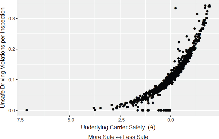
Figure C-2 plots unsafe driving violations per inspection against θ. There is a very close mapping between these two metrics, such that θ more or less returns the number of unsafe driving violations per inspection.
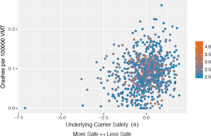
Figure C-3 plots crashes per 100,000 VMT against θ. There is a positive relationship but also very high variance about the least squares line (low R2). The Spearman correlation between crashes per 100000 VMT and θs from the binomial IRT is 0.23.
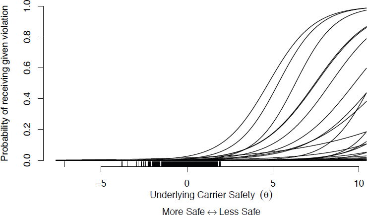
TABLE C-1 α, β, and Prevalence for the 20 Violations with the Highest α, Value Generated from Binomial Item Response Theory
| Description | Alpha | Beta | Prevalence |
|---|---|---|---|
| Speeding | 0.931 | –11.2 | 10 |
| Following too close | 0.871 | –5.5 | 3010 |
| Lane restriction violation | 0.839 | –4.5 | 8328 |
| State-local laws operating a CMV while texting | 0.833 | –8.9 | 95 |
| Inattentive driving | 0.771 | –11.0 | 12 |
| State-local laws speeding 6-10 miles per hour over limit | 0.760 | –3.6 | 18946 |
| Operating a CMV while texting | 0.734 | –9.6 | 47 |
| Driving a CMV while texting | 0.635 | –8.8 | 111 |
| Improper lane change | 0.631 | –5.3 | 3614 |
| Failing to use seat belt while operating a CMV | 0.627 | –4.7 | 6532 |
| State-local laws speeding 11-14 miles per hour over limit | 0.620 | –4.7 | 6629 |
| Using a handheld mobile telephone while operating a CMV | 0.568 | –5.5 | 2752 |
| Allowing or requiring driver to use a handheld mobile telephone | 0.565 | –10.4 | 20 |
| Failure to slow down approaching a railroad crossing | 0.540 | –11.4 | 7 |
| State-local laws speeding in work/construction zone | 0.530 | –5.8 | 2134 |
| Failing to stop at railroad crossing bus | 0.489 | –11.3 | 8 |
| State-local laws speeding 15+ miles per hour over limit | 0.459 | –5.3 | 3549 |
| Railroad grade crossing violation | 0.441 | –10.4 | 21 |
| Improper passing | 0.426 | –7.3 | 463 |
| Scheduling run to necessitate speeding | 0.400 | –10.7 | 15 |
NOTE: CMV, commercial motor vehicle.
REFERENCES
Furr, D.C. (2017). edstan: Stan models for item response theory, version 1.0.6. Available: https://CRAN.R-project.org/package=edstan [July 2017].
Stan Development Team. (2016). RStan: the R interface to Stan, version 2.14.1.Available: http://mc-stan.org [July 2017].


